| Issue |
A&A
Volume 690, October 2024
|
|
|---|---|---|
| Article Number | A380 | |
| Number of page(s) | 11 | |
| Section | Planets and planetary systems | |
| DOI | https://doi.org/10.1051/0004-6361/202450761 | |
| Published online | 22 October 2024 | |
Warm Jupiters around M dwarfs are great opportunities for extensive chemical, cloud, and haze characterisation with JWST
1
LESIA, Observatoire de Paris, Université PSL, Sorbonne Université, Université Paris Cité, CNRS,
5 place Jules Janssen,
92195
Meudon,
France
2
Laboratoire de Météorologie Dynamique, IPSL, CNRS, Sorbonne Université, Ecole Normale Supérieure, Université PSL, Ecole Polytechnique, Institut Polytechnique de Paris,
75005
Paris,
France
3
AIM, CEA, CNRS, Université Paris-Saclay, Université Paris Cité
91191
Gif-sur-Yvette,
France
4
Astrobiology Research Unit, Université de Liège,
Allée du 6 août 19,
Liège
4000,
Belgium
★ Corresponding author; This email address is being protected from spambots. You need JavaScript enabled to view it.
Received:
17
May
2024
Accepted:
27
August
2024
Abstract
Context. The known population of short-period giant exoplanets around M-dwarf stars is slowly growing. These planets present an extraordinary opportunity for atmospheric characterisation and defy our current understanding of planetary formation. Furthermore, clouds and hazes are ubiquitous in warm exoplanets, but their behaviour is still poorly understood.
Aims. We studied the case of a standard warm Jupiter around an M-dwarf star to show the opportunity of this exoplanet population for atmospheric characterisation. We aimed to derive the cloud, haze, and chemical budget of such planets using JWST.
Methods. We leveraged a 3D global climate model, the generic PCM, to simulate the cloudy and cloud-free atmosphere of warm Jupiters around an M dwarf. We then post-processed our simulations to produce spectral phase curves and transit spectra as would be seen with JWST.
Results. We show that, using the amplitude and offset of the spectral phase curves, we can directly infer the presence of clouds and hazes in the atmosphere of such giant planets. Chemical characterisation of multiple species is possible with an unprecedented signal- to-noise ratio, using the transit spectrum in one single visit. In such atmospheres, NH3 could be detected for the first time in a giant exoplanet. We make the case that these planets are key to understanding the cloud and haze budget in warm giants. Finally, such planets are targets of great interest for Ariel.
Key words: planets and satellites: atmospheres / planets and satellites: composition
© The Authors 2024
 Open Access article, published by EDP Sciences, under the terms of the Creative Commons Attribution License (https://creativecommons.org/licenses/by/4.0), which permits unrestricted use, distribution, and reproduction in any medium, provided the original work is properly cited.
This article is published in open access under the Subscribe to Open model. This email address is being protected from spambots. You need JavaScript enabled to view it. to support open access publication.
1 Introduction
M-dwarf stars are promising hosts for exoplanets and their atmospheric characterisation, as they are the coolest, smallest, and most abundant stars in our neighbourhood (Bochanski et al. 2010). This is referred to as the ‘small star opportunity’ (Triaud 2021). Thus, a few surveys have been designed to study such systems (such as SPECULOOS, Delrez et al. 2018; Triaud et al. 2023, PINES Tamburo et al. 2022, EDEN, Gibbs et al. 2020, MEarth, Nutzman & Charbonneau 2008, and others that use TESS, Ricker et al. 2015), leading to major discoveries of rocky planets (for instance, the TRAPPIST-1 system, Gillon et al. 2016, 2017). While close-in planets orbiting around M stars are rare, at least a dozen close-in giant planets have been discovered (Triaud et al. 2023). Due to the favourable ratio of the size of the planet to the size of the star, atmospheric characterisation of such targets is more favourable than around F, G, and K stars. Nevertheless, the question of how these giant planets formed around low-mass stars is still a mystery. Indeed, core accretion models predict a low probability of formation of giant planets around such stars (Schlecker et al. 2022). Thus, other formation pathways, such as gravitational instabilities followed by inward migration, might be at play in these systems (Morales et al. 2019; Liu & Ji 2020; Kennedy & Kenyon 2008).
Clouds and hazes are ubiquitous in the atmospheres of giant planets. In particular, clouds (i.e. particles formed through the condensation of gases) have multiple absorption signatures in the infrared (Grant et al. 2023; Morley et al. 2014; Dyrek et al. 2024b; Miles et al. 2023) and are also known to weaken emergent spectral lines (Sing et al. 2016). Hazes (i.e. particles formed through complex photochemical reactions originating from the stellar UV flux) could explain super-Rayleigh slopes seen in transit spectra (Ohno & Kawashima 2020) and are thought to dominate over clouds in cooler atmospheres (Gao et al. 2021; Lavvas & Koskinen 2017; Arfaux & Lavvas 2022). Where clouds produce a greenhouse effect in hot atmospheres (Teinturier et al. 2024), hazes are thought to produce an anti-greenhouse effect (McKay et al. 1989). Using a 3D global climate model (GCM), Steinrueck et al. (2023) modelled the radiative feedback of hazes on a hot Jupiter and found that regardless of the assumed radiative properties of the hazes, a strong dayside temperature inversion forms at low pressures. However, they were unable to match the transmission spectra. For sub-Neptunes, featureless transit spectra in the near-infrared, probably due to high thick clouds or hazes, have been observed (Kreidberg et al. 2014) and modelled (Charnay et al. 2015a), but the spectral characterisation of the composition and size distribution of the aerosols is still lacking. Thus, clouds and hazes are still fairly unknown on giant exoplanets.
Now that we have entered the JWST era, precise atmospheric characterisations of hot Jupiters are possible both in emission and transmission spectroscopy, yielding unprecedented signal-to-noise ratios (S/Ns) and various atmospheric features (Alderson et al. 2023; Bell et al. 2024; Feinstein et al. 2023; Rustamkulov et al. 2023; JWST Transiting Exoplanet Community Early Release Science Team et al. 2023; Tsai et al. 2023; Coulombe et al. 2023; Mikal-Evans et al. 2023; Grant et al. 2023). Transit spectroscopy on giant planets around M- dwarf stars is currently undergoing for eight systems (Program 3171, Kanodia et al. (2023), Program 5799, Garcia et al. (2024), Program 5863, Murray et al. (2024)), but to date, emission spectroscopy and phase curves have not yet been scheduled. However, short-period giant planets around M-dwarfs are prime targets for a complete energetic budget, albedo, chemical, cloud, and haze characterisation either using NIRSPec-PRISM (to probe both thermal and reflected light without saturation of the detector) or in thermal emission with MIRI-LRS. In particular, the M-dwarfs do not saturate the NIRSPec-PRISM detector, which makes them advantageous compared to many exoplanets’ host stars for which PRISM cannot be used. Moreover, the launch of PLATO and Ariel in the coming years will yield longer phase curves than the one obtained by JWST, at optical and near- to mid-infrared wavelengths.
In particular, as M-dwarf stars are cool, the giant planets orbiting them are in the temperate temperature regime (Triaud 2021). Thus, they can be used as proxies for hot sub-Neptunes with better S/N, transmission, and emission spectroscopic metrics (TSM and ESM) (Kempton et al. 2018). Therefore, insights into cloud and haze formation and composition that are very difficult or impossible to constrain on smaller planets (such as GJ-1214b, Kempton et al. 2023) could be obtained with these targets. In this paper, we investigate the potential of atmospheric characterisation with JWST for giant planets around M-dwarf stars using a GCM.
In Section 2, we describe the choice of the target and the numerical models used. We present our results in Section 3 and discuss and conclude this work in Section 4.
2 Methods
2.1 Target selection
In this paper, we focus on planets around M-dwarf stars with an equilibrium temperature below 800 K. These planets are a good analogue for warm sub-Neptunes and Neptunes (i.e. GJ 1214 b, GJ 436 b, and GJ 3470 b), but with better potential for atmospheric characterisation due to their size. In this temperature regime, we expect to be able to investigate hazes and clouds simultaneously. We show in Fig. 1 the population of confirmed (to-date) warm Jupiters around M-dwarf stars, in the orbital period-equilibrium temperature space, colour-coded using the Emission Spectroscopic Metric (ESM, Kempton et al. (2018)). To keep this study generic, we chose a target with a good enough ESM and an orbital period of less than two days. We used this criterion because observing a phase curve of more than two days seemed improbable in the near future with current observing facilities. This left us with few choices, even though confirmation of numerous planetary candidates satisfying these criteria is currently ongoing (the SPECULOOS collaboration, private comm., Kanodia et al. 2024), which will widen the parameter space. Thus, we chose to model TOI-519 b (Parviainen et al. 2021; Kagetani et al. 2023; Hartman et al. 2023) as a benchmark of warm Jupiters around M-dwarf stars amenable for cloud and haze characterisation. Moreover, we state that TOI- 519 b is observable with JWST in all instrument modes, without saturation.
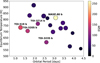 |
Fig. 1 Population of confirmed close-in gas giants around M-dwarf stars, in the orbital period-equilibrium temperature space. The colour bar represents the ESM, and the size of each dot is proportional to the planetary radius. We highlighted the five targets with the best ESM. |
2.2 General circulation model
This work uses the generic Planetary Climate Model (generic PCM). This model couples a dynamical core which solves the 3D primitive equations of meteorology on a finite difference longitude-latitude grid (Hourdin et al. 2006), and different physical parameterizations of physical phenomena without assumptions made regarding the planet it simulates. In particular, this model has been used to simulate the climate of giant planets (Spiga et al. 2020; Cabanes et al. 2020; Bardet et al. 2021, 2022; Milcareck et al. 2024), telluric and small exoplanets (Charnay et al. 2015b,a, 2021a; Leconte et al. 2013; Turbet et al. 2023) and recently Hot Jupiters (Teinturier et al. 2024). The physical parameterizations encompass a radiative transfer scheme based on the k-correlated method and the Toon et al. (1989) algorithm, vertical turbulent mixing, and an adiabatic temperature adjustment scheme for convectively unstable regions. Moreover, the model takes into account cloud formation, sedimentation, advection, and radiative feedbacks as described in Teinturier et al. (2024). A sponge layer in the four upper layers of the atmosphere is used to damp nonphysical oscillations that could be present due to the model’s closed-lid upper boundary.
2.3 Simulation set-up
We used the generic PCM to model TOI-519 baround its M3.5 star (T⋆ = 3300 K, R⋆ = 0.35 R⊙, Kagetani et al. 2023). The planet was modelled on a tidally locked, circular orbit at a distance of 0.015 AU, with an orbital period of 1.265 days (Kagetani et al. 2023). The planetary radius, Rp , and the gravity are fixed at 1.03 RJup and 10.76 m s−2, respectively, according to the values derived in Kagetani et al. (2023). We also used the values of 2.346 g mol−1 and 12305 J K−1 kg−1 for the mean molecular weight and the specific heat capacity of the atmosphere. The internal temperature, Tint, was set to 100 K.
We initialised the model following the procedure described in Teinturier et al. (2024) and briefly summarised hereafter. We used the Exo-REM code (Charnay et al. 2018; Blain et al. 2021) to compute vertical chemical profiles for H2 O, CO, CH4 , CO2, FeH, HCN, H2S, TiO, VO, Na, K, PH3 , and NH3 , assuming disequilibrium chemistry, a solar metallicity, and a vertical temperature profile (see Fig. A.1). The disequilibrium processes were computed using an analytical formalism, which compares the chemical time constants with the vertical mixing time, taken from Zahnle & Marley (2014), with an eddy mixing coefficient of 4.5 ×10⁷ m2 s−1. We used these profiles and the exo_k package (Leconte 2021) to create mixed, temperature-pressure-dependent k-tables with 16 Gauss-Legendre quadrature points. These k- tables and the temperature profile were fed into the 1D version of the generic PCM until it reached radiative balance. The outputted temperature profile was then used to initialise the 3D model, in a horizontally uniform way.
We used a horizontal resolution of 64x48 and 40 vertical layers, equally spaced in log-pressure between 80 bars and 10 Pa. The dynamical time step is 28.76 s, and the physical-radiative time step is 143.81 s. Overall, the set-up is highly similar to the one used in Teinturier et al. (2024).
Starting from a rest state (i.e. no winds), we ran a cloudless model for 3000 planetary years until the upper atmosphere reached a steady state. We then added clouds composed of KCl and Na2 S with a mean radius of 1 µm and a log-normal distribution in size of variance 0.1 and ran the simulation for an additional 500 planetary years. To initialise the clouds, we used the formulas of Morley et al. (2012) for the condensable vapour and started with no clouds (see Fig. A.2). The optical properties used are taken from Querry (1987) for KCl and from Montaner et al. (1979) and Khachai et al. (2009) for Na2S . We only considered these two cloud species, as they are the clouds expected to form in this temperature range. We neglected ZnS, which could also form, as the optical properties of ZnS clouds have negligible radiative contributions compared to the other two.
The cloud parametrisation used is the same as in Teinturier et al. (2024), where at each time step and in each grid cell, the saturation vapour pressure of the cloud species is computed using the condensation curves of KCl and Na2S and compared to the partial pressure of the gas. If the grid cell is saturated, condensable vapour condenses into a solid. Clouds can then be transported by the dynamics and/or experience sedimentation. Latent heat release from cloud condensation is also taken into account but is negligible in these atmospheres.
2.4 Simulations of observations using PandExo
We post-processed our simulations’ outputs using the Pytmosph3R code (Falco et al. 2022). We used the same opacities and spectral range as for the GCM runs but at a higher spectral resolution, equivalent to R ~ 500. Thus, for each GCM run, we produced spectral phase curves and a transit spectrum.
We then used the online version of PandExo Batalha et al. (2017) to estimate the noise of a single transit and eclipse as seen by JWST using NIRISS-SOSS, NIRSpec-PRISM, and MIRI- LRS. For the stellar spectrum, we used the default PHOENIX model for Teff = 3322 K, normalised to a J-mag = 12.847. Table 1 summarises the parameters that we used to compute the noise. For each instrument, we ran simulations using the cloudless and cloudy transmission and emission spectra output from the GCM runs. We also computed the photometric precision of the white light curve to derive the uncertainty of the timing offset of the phase curve of the planet for each instrument, following the methodology of Alegria & Serra (2006).
3 Results
3.1 Atmospheric structure
The atmospheric states obtained at the end of the simulations are similar to those of Hot Jupiters around G, F, or K stars (see Showman et al. (2020) for a review). We show in Fig. B.1 a longitude-latitude temperature map and the structure of the zonal wind for our cloudless and cloudy simulations. In both cases, an equatorial super-rotating jet is present and redistributes heat from the heated dayside to the cool nightside. An eastward shift of the hotspot from the substellar point is also seen, as is the strong temperature contrast between day and nightside. The impact of clouds on the thermal and dynamical structure is very similar to the findings of Teinturier et al. (2024), where the clouds have a net warming effect on the atmosphere (nightside warming by greenhouse effects dominates the cooling by albedo effect on the dayside), reduce the eastward shift of the hotpost, and decelerate the equatorial jet. Also seen is a modification of the structure of the high-latitude winds, which transition from prograde to retrograde jets due to the modification of the thermal gradients of the atmosphere by the radiative feedback of the clouds. We show the horizontal distribution of clouds in Fig. B.2, on a representative isobaric level. Clouds mostly form on the nightside and at mid-to-high latitudes, leaving a permanent low-latitude cloudless dayside.
Parameters used to compute the expected spectral precision on the transit and eclipse depth of TOI-519 b using NIRISS-SOSS, NIRSpec-PRISM, or MIRI-LRS.
3.2 Phase curves and secondary eclipses
We first compared the white light curve amplitude and offset derived from our two simulations for NIRSpec-PRISM and MIRI-LRS. As expected from previous studies (Parmentier et al. 2020, for instance), the phase curve amplitude increases and the offset decreases when clouds are added to the simulations. However, in this particular case of a giant planet around an M-dwarf star, the statistical significance with which these changes can be detected is greater than that for FGK hosts (see Fig. 2). This change is especially remarkable in the amplitude of the MIRI- LRS phase curve and the offsets with both instruments. Thus, even without leveraging the spectral dependence of the phase curve, such measurements should be sufficient to indicate the presence or lack of clouds.
Digging into the spectral shape of the phase curve (which probes different vertical depths), we observe drastic changes for wavelengths greater than 2 µm. Indeed, the spectral amplitudes of cloudy simulations are considerably stronger than in the cloudless case, and the spectral offsets subsequently lower. In the MIRI-LRS range, the offset is below 20°, whereas it is at least twice as large in the clear-sky simulation. This is also the case for NIRSpec-PRISM, with a stronger spectral variability. At shorter wavelengths (λ ≤ 2 µm), the amplitude level is low (≤200 ppm) but is still distinguishable between the two cases presented here. In particular, negative offsets at optical wavelengths are seen, due to the reflected light contribution that is enhanced in the presence of clouds. However, NIRSPec-PRISM’s precision at optical wavelengths impedes a clear detection of negative offsets as an indicator of cloud scattering contribution. Indeed, the reflected light component is of the order of ~10 ppm, which is the order of magnitude of the thermal component at these wavelengths. For completeness, we show a subset of spectral phase curves converted to brightness temperature in Appendix C.
The secondary eclipses are shown for NIRSpec-PRISM and MIRI-LRS at the bottom of Fig. 2. Multiple spectral features are seen with both instruments. At shorter wavelengths, the flux level is clearly detectable above 0.8 µm, and is twice as high as the flux observed on WASP-80 b (Bell et al. 2023). For wavelengths above 3 µm, the effect of clouds is seen as an increase in flux with regard to the cloudless case. Thus, warm giants around M-dwarf stars are prime targets for emission spectroscopy with JWST.
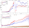 |
Fig. 2 Spectral features of the phase curve and secondary eclipses. Top: amplitude and offset of the phase curves simulated with NIRSpec-PRISM and MIRI-LRS. Bottom: secondary eclipses in the NIRSpec-Prism and MIRI-LRS range. The dots represent the NIRSpec-PRISM range, while the diamonds are the MIRI-LRS range. Cloudless simulations are in blue, and cloudy simulations are in red. In all observing modes, the effect of clouds is unambiguously detectable. The zoomed-in subplot provides a better visualisation of NIRSpec-PRISM’s shorter wavelengths. The lines in which horizontal error bars encompass the entirety of the instrument bands correspond respectively to the white amplitude and offset of the instrument. Contributions from major chemical species are shown at the bottoms of the plot and zoomed-in subplot. In the right panel, the shaded region corresponds to a constant error (introduced by the model’s coarse horizontal resolution) of ∼2.8125° on the offset location, as each longitudinal grid cell spans an angular resolution of 5.625°. In the bottom panel, the shaded regions around the spectra correspond to the native resolution of the instruments and their errors. |
3.3 Using the optical offset for haze detection
As shown in Fig. 2 for TOI-519 b, negative offsets due to clouds are observed for wavelengths below 1 µm, as the dayside is cloudless and the nightside is cloudy (Fig. B.2). Thus, if one observes null offsets in the optical range, this would indicate the presence of dayside reflective materials, such as hazes. We investigated the limit of this hypothesis by running additional simulations of a cloudy TOI-519 b, but lowering the irradiation temperature (thus cooling the planet) until cloud formation occurs at the substellar point. Dayside clouds appear for an irradiation temperature of around 775 K. The geometric albedo increases by 5, 11, and 18% compared with the reference case; these simulations are shown in Fig. 3. However, null optical offsets require more dayside clouds and are seen for lower irradiation temperatures (Fig. 3). This behaviour is understandable; when we start to form dayside clouds, we already have an opaque cloud cover at the western terminator that determines the location of the offset. Thus, the phase curve’s optical offset could help constrain the haze’s existence only for irradiation temperatures above ∼700 K. This is the case for TOI-3714 b, TOI-5205 b, and TOI-519 b. For lower irradiation temperatures, null optical offsets could be due to hazes, dayside clouds, or both, without the possibility of distinguishing between the two as for TOI-3235 b. In the unlikely case where cloud formation is prevented, the presence of hazes over a clear sky could be inferred by measuring the Bond albedo, as done for GJ 1214 b with a MIRI-LRS phase curve (Kempton et al. 2023).
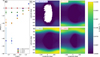 |
Fig. 3 Phase curve offset and link to the dayside cloud structures for different irradiation temperatures. (a): NIRSpec optical wavelength phase curve offsets. Simulations with different irradiation temperatures are represented with different colours. (b): Column mass of clouds (both Na2S and KCl are considered in these maps) for the same irradiation temperatures as in the left panel. |
3.4 Transit spectra
We show in Fig. 4 the transit spectra computed from our cloudless and cloudy simulations and noised with PandExo for NIRISS-SOSS, NIRSpec-PRISM, and MIRI-LRS. In all the spectral ranges shown (0.6–10.5 µm), the cloudy and cloudless simulations are offset by 500–1200 ppm. Thus, the absolute flux level of the transit spectrum is indicative of cloudiness. NIRSpec-PRISM especially stands out thanks to its combination of broad wavelength coverage and excellent precision.
The ∼3.3 µm methane feature is significantly detected with this instrument, allowing strong chemical constraints to be obtained at the terminator of the planet. CH4 has already been detected in the atmosphere of warm Jupiters, both in transit and emission spectroscopy, using the NIRCAM F322W2 grism (Bell et al. 2023). However, high spectral resolution was needed to constrain CH4, mostly because of the low flux level of the observed planet. Here, we argue that the low spectral resolution of NIRSpec-PRISM is sufficient because of the strong transit depth (∼9.3 % for TOI-519 b compared to ∼3% for WASP-80b, for instance).
Water features are also seen at shorter wavelengths for NIRSpec-PRISM and in the MIRI-LRS range. Determination of its abundance could help constrain the C/O ratio of the planet. Interestingly, for our assumed chemical composition, hints of CO and CO2 around 4–4.5 µm appear. Moreover, NH3 displays several absorption features at 1.5, 1.9, 3.0, and 6.2 µm. These features might be small and hidden by overlapping absorption bands of H2O or CH4 , for instance. However, detection of NH3 with transit spectroscopy has not been done so far (to our knowledge), and our case study of warm Jupiters around M- dwarf stars would be a prime target for such investigation. In particular, NH3 would only be detectable if vertical mixing is active and not in the equilibrium chemistry scenario. Thus, transit spectroscopy could provide information about disequilibrium chemistry mechanisms in these atmospheres. Finally, depending on the spectral binning used with NIRSpec-PRISM, a clear detection and characterisation of the potassium at 0.77 µm is feasible.
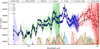 |
Fig. 4 Transit spectra for our cloudless (dots) and cloudy (diamonds) simulations, noised with PandExo, for NIRISS-SOSS (green, with a bin width of 0.08 µm), NIRSpec-PRISM (blue, with a bin width of 0.1 µm), and MIRI-LRS (red, with a bin width of 0.35 µm), corresponding to one transit with each instrument. The shaded regions around the spectra correspond to the native resolution of the instruments and their errors, before binning. The GCM post-processed transit spectra are in black, with a solid line for the cloudless case and a dashed line for the cloudy case. Contributions from major chemical absorbers are shown at the bottom of the plot. |
4 Discussion and concluding remarks
In this work, we investigate the spectral observations of a giant planet around an M-dwarf star, as would be seen with JWST. We show that CH4 and H2O should be easily detected with NIRSpec- PRISM and MIRI-LRS in one single transit. Hints of NH3, CO, and CO2 are also detectable. These measurements could help constrain the C/O ratio and explain the formation pathway of such objects (Öberg et al. 2011). Depending on the value of the C/O, C/H, and O/H ratios, constraints could also be placed on the migration mechanism (Madhusudhan et al. 2014).
Measuring a spectral phase curve will allow unprecedented constraints on the cloud and chemical budgets of these giant planets. The spectral amplitude and offset will reveal the presence or absence of clouds. Depending on the target, one observing mode might be more favourable than the other. For the special case of TOI-519 b, we recommend a MIRI-LRS phase curve first, followed by a NIRSpec-PRISM one, as the S/N of these observations is high. Furthermore, it is worth noting that if the LRS fixed-slit mode demonstrates significantly higher sensitivity (as proposed by the calibration program GO 6219; PIs Dyrek & Lagage, Dyrek et al. 2024a) than the slitless mode for cooler and fainter stars, such as TOI-519, we can anticipate even greater precision. This enhanced precision would enable us to discern an even wider range of atmospheric scenarios.
In this work, we did not consider the G395H filter despite its wide use for atmospheric characterisation (Alderson et al. 2023; Smith et al. 2024). As shown previously, the lower spectral resolution of PRISM is sufficient to yield a clear detection of CH4 and also allows a large spectral range to be probed, including reflected light. Thus, using the G395H filter would yield great constraints on the carbon chemistry budget in these atmospheres, but PRISM is better equipped because of its broad wavelength coverage.
Finally, we did not consider hazes in our modelling, which are expected to be present on the dayside of such planets due to photochemistry (Steinrueck et al. 2023). As shown in Fig. B.2, our simulated dayside is cloudless. Thus, if observations yield a null offset of the phase curve at optical wavelengths, this would be strong evidence of the presence of such hazes, whereas negative optical offsets would indicate a clear (of clouds and hazes) dayside and a cloudy western terminator. However, our additional simulations highlight the existence of a thermal transition from a negative to a null optical offset due to an enhanced abundance of dayside clouds.
Nor did we consider stellar activity, which could mitigate the quality of these observations, as M-dwarf stars are known to exhibit spots and flares (Rackham et al. 2023). Thus, our estimated spectra are optimistic.
We emphasise that the climate model used in this study, the generic PCM, is well suited for flexible and fast simulations of giant planets around any stellar type. In this paper, we present the first 3D atmospheric study of a giant planet around an M-dwarf star.
Finally, the growing population of giant planets around M- dwarf stars are prime candidates for the Ariel space telescope (Tinetti et al. 2018), which will survey more than 1000 exoplanets and dedicate 10% of its time to phase curves (Charnay et al. 2021b). Ariel’s spectral coverage from 0.7 to 7.8 µm, combined with its ability to observe relatively long phase curves (up to 5 days), makes it ideal for probing this population of exoplanets.
Acknowledgements
This work has been granted access to the HPC resources of MesoPSL financed byb the Region Ile de France and the project Equip@Meso (reference ANR-10-EQPX-29-01) of the programme Investissements d’Avenir supervised by the Agence Nationale pour la Recherche. This work was supported by CNES, focused on AIRS on Ariel. E.D. acknowledges support from the innovation and research Horizon 2020 program in the context of the Marie Sklodowska-Curie subvention 945298. L.T. and E.D. strongly thank the creators of https://makeitmeme.com for bringing a lot of joy into the writing of this paper. The authors thank the anonymous referee for constructive remarks that enhanced the quality of this work.
Appendix A Initialisation
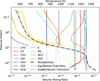 |
Fig. A.1 Chemical (coloured lines) and temperature (black dotted line) profiles derived from Exo-REM. The solid lines correspond to disequilibrium abundances and the dashed lines to chemical equilibrium abundances. The atmosphere is dominated by CH4 and not CO because of the low temperature. Although they are included in the computation, TiO and VO mixing ratios are negligible and do not appear on the plotted scale. |
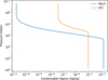 |
Fig. A.2 Condensable vapour profile of KCl and Na2S used at initialisation. We start with no clouds and only condensable vapour in the atmosphere. |
Appendix B Atmospheric states
In this section, we show a few maps of the dynamical and thermal structure modelled with the generic PCM. Fig. B.1 shows longitude-latitude temperature maps and zonal-mean zonal winds maps for our cloudless and cloudy simulations. In both cases, we observe a strong day-night temperature contrast and an eastward shift of the hotspot with regard to the sub-stellar location. Between a cloudy and cloudless atmosphere, we observe a reduction in the hotspot offset, correlated with the reduction of the spectral phase curves offset shown in Fig.C.1,C.2. We also observe a super-rotating, eastward, equatorial jet and a change in the wind structure at high latitudes between the two simulations. This is due to the radiative feedback of clouds, which alters the meridional temperature gradients (see Teinturier et al. (2024) for a more thorough description).
We also show longitude-latitude maps of the distribution of the clouds in Fig. B.2.
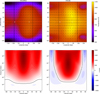 |
Fig. B.1 Thermal and wind structure of our cloudless and cloudy simulations of TOI-519 b. Top: longitude-latitude temperature map at a pressure of 25 mbar, averaged in time over the last 100 years. The black arrows represent the wind field, with the size of the arrow proportional to the strength of the wind. The vertical dashed black lines denote the terminators (longitude = ±90°). The white cross and dot represent the equatorial maxima and minima of temperature. Bottom: Zonal mean zonal wind (averaged in time over the last 100 years). The black line denotes the 0 m.s−1 level. The left panels represent the cloudless simulation while the right panels represent the cloudy simulation, including KCl and Na2S clouds. |
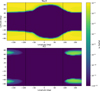 |
Fig. B.2 Horizontal maps of clouds at a pressure of 25 mbars. The top panel displays the Na2S cloud distribution while the bottom panel displays the KCl distribution. Due to the lower condensation temperature of KCl , we only observe its formation on the night-side polar vortices whilst Na2S uniformly forms at latitudes higher than ± 40° on the nightside, and at higher latitudes on the dayside. |
Appendix C Phase curves
We show here a subset of the spectral phase curves computed from the cloudy and cloudless simulation on the NIRSpec- PRISM and MIRI-LRS range.
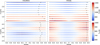 |
Fig. C.1 Cloudless (left) and cloudy (right) phase curves on the NIRSpec-PRISM spectral range, converted to planetary brightness temperature. The black crosses indicate the phase of the maximum flux for a given wavelength (i.e. the spectral offsets). Phase 0 corresponds to the night side (i.e. the transit event). |
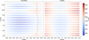 |
Fig. C.2 Cloudless (left) and cloudy (right) phase curves on the MIRI-LRS spectral range, converted to planetary brightness temperature. The black crosses indicate the phase of the maximum flux for a given wavelength (i.e. the spectral offsets). Phase 0 corresponds to the night side (i.e. the transit event). |
References
- Alderson, L., Wakeford, H. R., Alam, M. K., et al. 2023, Nature, 614, 664 [NASA ADS] [CrossRef] [Google Scholar]
- Alegria, F. C., & Serra, A. C. 2006, in 2006 IEEE Instrumentation and Measure392 ment Technology Conference Proceedings, 1643 [CrossRef] [Google Scholar]
- Arfaux, A., & Lavvas, P. 2022, MNRAS, 515, 4753 [NASA ADS] [CrossRef] [Google Scholar]
- Bardet, D., Spiga, A., Guerlet, S., et al. 2021, Icarus, 354, 114042 [Google Scholar]
- Bardet, D., Spiga, A., & Guerlet, S. 2022, Nature Astronomy, 6, 804 [NASA ADS] [CrossRef] [Google Scholar]
- Batalha, N. E., Mandell, A., Pontoppidan, K., et al. 2017, PASP, 129, 064501 [Google Scholar]
- Bell, T. J., Welbanks, L., Schlawin, E., et al. 2023, Nature, 623, 709 [Google Scholar]
- Bell, T. J., Crouzet, N., Cubillos, P. E., et al. 2024, Nat. Astron., 8, 1 [Google Scholar]
- Blain, D., Charnay, B., & Bézard, B. 2021, A&A, 646, A15 [EDP Sciences] [Google Scholar]
- Bochanski, J. J., Hawley, S. L., Covey, K. R., et al. 2010, AJ, 139, 2679 [NASA ADS] [CrossRef] [Google Scholar]
- Cabanes, S., Spiga, A., & Young, R. M. B. 2020, Icarus, 345, 113705 [NASA ADS] [CrossRef] [Google Scholar]
- Charnay, B., Meadows, V., & Leconte, J. 2015a, ApJ, 813, 15 [Google Scholar]
- Charnay, B., Meadows, V., Misra, A., et al. 2015b, AJ, 813, L1 [NASA ADS] [Google Scholar]
- Charnay, B., Bézard, B., Baudino, J.-L., et al. 2018, AJ, 854, 172 [NASA ADS] [Google Scholar]
- Charnay, B., Blain, D., Bézard, B., et al. 2021a, A&A, 646, A171 [NASA ADS] [CrossRef] [EDP Sciences] [Google Scholar]
- Charnay, B., Mendonça, J. M., Kreidberg, L., et al. 2021b, arXiv e-prints [arXiv:2102.06523] [Google Scholar]
- Coulombe, L.-P., Benneke, B., Challener, R., et al. 2023, Nature, 620, 292 [NASA ADS] [CrossRef] [Google Scholar]
- Delrez, L., Gillon, M., Queloz, D., et al. 2018, SPIE, 10700, 107001I [NASA ADS] [Google Scholar]
- Dyrek, A., Lagage, P.-O., Bell, T. J., et al. 2024a, JWST Proposal. Cycle 3, 6219 [Google Scholar]
- Dyrek, A., Min, M., Decin, L., et al. 2024b, Nature, 625, 51 [Google Scholar]
- Falco, A., Zingales, T., Pluriel, W., & Leconte, J. 2022, A&A, 658, A41 [NASA ADS] [CrossRef] [EDP Sciences] [Google Scholar]
- Feinstein, A. D., Radica, M., Welbanks, L., et al. 2023, Nature, 614, 670 [NASA ADS] [CrossRef] [Google Scholar]
- Gao, P., Wakeford, H. R., Moran, S. E., & Parmentier, V. 2021, J. Geophys. Res. Planets, 126, e2020JE006655 [CrossRef] [Google Scholar]
- Garcia, L., Charnay, B., Rackham, B., et al. 2024, JWST Proposal. Cycle 3, 5799 [Google Scholar]
- Gibbs, A., Bixel, A., Rackham, B. V., et al. 2020, AJ, 159, 169 [NASA ADS] [CrossRef] [Google Scholar]
- Gillon, M., Jehin, E., Lederer, S. M., et al. 2016, Nature, 533, 221 [Google Scholar]
- Gillon, M., Triaud, A. H. M. J., Demory, B.-O., et al. 2017, Nature, 542, 456 [NASA ADS] [CrossRef] [Google Scholar]
- Grant, D., Lewis, N. K., Wakeford, H. R., et al. 2023, ApJ, 956, L32 [NASA ADS] [CrossRef] [Google Scholar]
- Hartman, J. D., Bakos, G. A., Csubry, Z., et al. 2023, AJ, 166, 163 [NASA ADS] [CrossRef] [Google Scholar]
- Hourdin, F., Musat, I., Bony, S., et al. 2006, Clim. Dyn., 27, 787 [Google Scholar]
- JWST Transiting Exoplanet Community Early Release Science Team, Ahrer, E.-M., Alderson, L., et al. 2023, Nature, 614, 649 [NASA ADS] [CrossRef] [Google Scholar]
- Kagetani, T., Narita, N., Kimura, T., et al. 2023, PASJ, 75, 713 [NASA ADS] [CrossRef] [Google Scholar]
- Kanodia, S., Canas, C., Libby-Roberts, J., et al. 2023, JWST Proposal. Cycle 2, 3171 [Google Scholar]
- Kanodia, S., Cañas, C. I., Mahadevan, S., et al. 2024, arXiv e-prints [arXiv:2402.04946] [Google Scholar]
- Kempton, E. M.-R., Bean, J. L., Louie, D. R., et al. 2018, PASP, 130, 114401 [CrossRef] [Google Scholar]
- Kempton, E. M. R., Zhang, M., Bean, J. L., et al. 2023, Nature, 620, 67 [NASA ADS] [CrossRef] [Google Scholar]
- Kennedy, G. M., & Kenyon, S. J. 2008, ApJ, 673, 502 [Google Scholar]
- Khachai, H., Khenata, R., Bouhemadou, A., et al. 2009, J. Phys. Condensed Matter, 21, 095404 [NASA ADS] [CrossRef] [Google Scholar]
- Kreidberg, L., Bean, J. L., Désert, J.-M., et al. 2014, Nature, 505, 69 [Google Scholar]
- Lavvas, P., & Koskinen, T. 2017, ApJ, 847, 32 [NASA ADS] [CrossRef] [Google Scholar]
- Leconte, J. 2021, A&A, 645, A20 [NASA ADS] [CrossRef] [EDP Sciences] [Google Scholar]
- Leconte, J., Forget, F., Charnay, B., et al. 2013, A&A, 554, A69 [NASA ADS] [CrossRef] [EDP Sciences] [Google Scholar]
- Liu, B., & Ji, J. 2020, Res. Astron. Astrophys., 20, 164 [Google Scholar]
- Madhusudhan, N., Amin, M. A., & Kennedy, G. M. 2014, ApJ, 794, L12 [Google Scholar]
- McKay, C. P., Pollack, J. B., & Courtin, R. 1989, Icarus, 80, 23 [NASA ADS] [CrossRef] [Google Scholar]
- Mikal-Evans, T., Sing, D. K., Dong, J., et al. 2023, ApJ, 943, L17 [CrossRef] [Google Scholar]
- Milcareck, G., Guerlet, S., Montmessin, F., et al. 2024, A&A [Google Scholar]
- Miles, B. E., Biller, B. A., Patapis, P., et al. 2023, ApJ, 946, L6 [NASA ADS] [CrossRef] [Google Scholar]
- Montaner, A., Galtier, M., Benoit, C., & Bill, H. 1979, Phys. Status Solidi a, 52, 597 [NASA ADS] [CrossRef] [Google Scholar]
- Morales, J. C., Mustill, A. J., Ribas, I., et al. 2019, Science, 365, 1441 [Google Scholar]
- Morley, C. V., Fortney, J. J., Marley, M. S., et al. 2012, ApJ, 756, 172 [NASA ADS] [CrossRef] [Google Scholar]
- Morley, C. V., Marley, M. S., Fortney, J. J., et al. 2014, ApJ, 787, 78 [Google Scholar]
- Murray, C. A., Berta-Thompson, Z. K., Canas, C., et al. 2024, JWST Proposal. Cycle 3, 5863 [Google Scholar]
- Nutzman, P., & Charbonneau, D. 2008, PASP, 120, 317 [Google Scholar]
- Ohno, K., & Kawashima, Y. 2020, ApJ, 895, L47 [NASA ADS] [CrossRef] [Google Scholar]
- Öberg, K. I., Murray-Clay, R., & Bergin, E. A. 2011, ApJ, 743, L16 [Google Scholar]
- Parmentier, V., Showman, A. P., & Fortney, J. J. 2020, MNRAS, 501, 78 [NASA ADS] [CrossRef] [Google Scholar]
- Parviainen, H., Palle, E., Zapatero-Osorio, M. R., et al. 2021, A&A, 645, A16 [NASA ADS] [CrossRef] [EDP Sciences] [Google Scholar]
- Querry, M. 1987, Optical Constants of Minerals and Other Materials from the Millimeter to the Ultraviolet (USA: Chemical Research, Development & Engineering Center) [Google Scholar]
- Rackham, B. V., Espinoza, N., Berdyugina, S. V., et al. 2023, RAS Tech. Instrum., 2, 148 [NASA ADS] [CrossRef] [Google Scholar]
- Ricker, G. R., Winn, J. N., Vanderspek, R., et al. 2015, J. Astron. Telesc. Instrum. Syst., 1, 014003 [Google Scholar]
- Rustamkulov, Z., Sing, D. K., Mukherjee, S., et al. 2023, Nature, 614, 659 [NASA ADS] [CrossRef] [Google Scholar]
- Schlecker, M., Burn, R., Sabotta, S., et al. 2022, A&A, 664, A180 [NASA ADS] [CrossRef] [EDP Sciences] [Google Scholar]
- Showman, A. P., Tan, X., & Parmentier, V. 2020, Space Sci. Rev., 216, 139 [Google Scholar]
- Sing, D. K., Fortney, J. J., Nikolov, N., et al. 2016, Nature, 529, 59 [Google Scholar]
- Smith, P. C. B., Line, M. R., Bean, J. L., et al. 2024, AJ, 167, 110 [NASA ADS] [CrossRef] [Google Scholar]
- Spiga, A., Guerlet, S., Millour, E., et al. 2020, Icarus, 335, 113377 [Google Scholar]
- Steinrueck, M. E., Koskinen, T., Lavvas, P., et al. 2023, ApJ, 951, 117 [NASA ADS] [CrossRef] [Google Scholar]
- Tamburo, P., Muirhead, P. S., McCarthy, A. M., et al. 2022, AJ, 163, 253 [NASA ADS] [CrossRef] [Google Scholar]
- Teinturier, L., Charnay, B., Spiga, A., et al. 2024, A&A, 683, A231 [NASA ADS] [CrossRef] [EDP Sciences] [Google Scholar]
- Tinetti, G., Drossart, P., Eccleston, P., et al. 2018, Exp. Astron., 46, 135 [NASA ADS] [CrossRef] [Google Scholar]
- Toon, O. B., McKay, C. P., Ackerman, T. P., & Santhanam, K. 1989, J. Geophys. Res., 94, 16287 [Google Scholar]
- Triaud, A. H. M. J. 2021, ExoFrontiers: Big Questions in Exoplanetary Science, Chap. 6, ed. N. Madhusudhan (Bristol: IOP Publishing) [Google Scholar]
- Triaud, A. H. M. J., Dransfield, G., Kagetani, T., et al. 2023, MNRAS, 525, L98 [Google Scholar]
- Tsai, S.-M., Lee, E. K. H., Powell, D., et al. 2023, Nature, 617, 483 [CrossRef] [Google Scholar]
- Turbet, M., Fauchez, T. J., Leconte, J., et al. 2023, A&A, 679, A126 [NASA ADS] [CrossRef] [EDP Sciences] [Google Scholar]
- Zahnle, K. J., & Marley, M. S. 2014, ApJ, 797, 41 [CrossRef] [Google Scholar]
All Tables
Parameters used to compute the expected spectral precision on the transit and eclipse depth of TOI-519 b using NIRISS-SOSS, NIRSpec-PRISM, or MIRI-LRS.
All Figures
|
Fig. 1 Population of confirmed close-in gas giants around M-dwarf stars, in the orbital period-equilibrium temperature space. The colour bar represents the ESM, and the size of each dot is proportional to the planetary radius. We highlighted the five targets with the best ESM. |
| In the text | |
|
Fig. 2 Spectral features of the phase curve and secondary eclipses. Top: amplitude and offset of the phase curves simulated with NIRSpec-PRISM and MIRI-LRS. Bottom: secondary eclipses in the NIRSpec-Prism and MIRI-LRS range. The dots represent the NIRSpec-PRISM range, while the diamonds are the MIRI-LRS range. Cloudless simulations are in blue, and cloudy simulations are in red. In all observing modes, the effect of clouds is unambiguously detectable. The zoomed-in subplot provides a better visualisation of NIRSpec-PRISM’s shorter wavelengths. The lines in which horizontal error bars encompass the entirety of the instrument bands correspond respectively to the white amplitude and offset of the instrument. Contributions from major chemical species are shown at the bottoms of the plot and zoomed-in subplot. In the right panel, the shaded region corresponds to a constant error (introduced by the model’s coarse horizontal resolution) of ∼2.8125° on the offset location, as each longitudinal grid cell spans an angular resolution of 5.625°. In the bottom panel, the shaded regions around the spectra correspond to the native resolution of the instruments and their errors. |
| In the text | |
|
Fig. 3 Phase curve offset and link to the dayside cloud structures for different irradiation temperatures. (a): NIRSpec optical wavelength phase curve offsets. Simulations with different irradiation temperatures are represented with different colours. (b): Column mass of clouds (both Na2S and KCl are considered in these maps) for the same irradiation temperatures as in the left panel. |
| In the text | |
|
Fig. 4 Transit spectra for our cloudless (dots) and cloudy (diamonds) simulations, noised with PandExo, for NIRISS-SOSS (green, with a bin width of 0.08 µm), NIRSpec-PRISM (blue, with a bin width of 0.1 µm), and MIRI-LRS (red, with a bin width of 0.35 µm), corresponding to one transit with each instrument. The shaded regions around the spectra correspond to the native resolution of the instruments and their errors, before binning. The GCM post-processed transit spectra are in black, with a solid line for the cloudless case and a dashed line for the cloudy case. Contributions from major chemical absorbers are shown at the bottom of the plot. |
| In the text | |
|
Fig. A.1 Chemical (coloured lines) and temperature (black dotted line) profiles derived from Exo-REM. The solid lines correspond to disequilibrium abundances and the dashed lines to chemical equilibrium abundances. The atmosphere is dominated by CH4 and not CO because of the low temperature. Although they are included in the computation, TiO and VO mixing ratios are negligible and do not appear on the plotted scale. |
| In the text | |
|
Fig. A.2 Condensable vapour profile of KCl and Na2S used at initialisation. We start with no clouds and only condensable vapour in the atmosphere. |
| In the text | |
|
Fig. B.1 Thermal and wind structure of our cloudless and cloudy simulations of TOI-519 b. Top: longitude-latitude temperature map at a pressure of 25 mbar, averaged in time over the last 100 years. The black arrows represent the wind field, with the size of the arrow proportional to the strength of the wind. The vertical dashed black lines denote the terminators (longitude = ±90°). The white cross and dot represent the equatorial maxima and minima of temperature. Bottom: Zonal mean zonal wind (averaged in time over the last 100 years). The black line denotes the 0 m.s−1 level. The left panels represent the cloudless simulation while the right panels represent the cloudy simulation, including KCl and Na2S clouds. |
| In the text | |
|
Fig. B.2 Horizontal maps of clouds at a pressure of 25 mbars. The top panel displays the Na2S cloud distribution while the bottom panel displays the KCl distribution. Due to the lower condensation temperature of KCl , we only observe its formation on the night-side polar vortices whilst Na2S uniformly forms at latitudes higher than ± 40° on the nightside, and at higher latitudes on the dayside. |
| In the text | |
|
Fig. C.1 Cloudless (left) and cloudy (right) phase curves on the NIRSpec-PRISM spectral range, converted to planetary brightness temperature. The black crosses indicate the phase of the maximum flux for a given wavelength (i.e. the spectral offsets). Phase 0 corresponds to the night side (i.e. the transit event). |
| In the text | |
|
Fig. C.2 Cloudless (left) and cloudy (right) phase curves on the MIRI-LRS spectral range, converted to planetary brightness temperature. The black crosses indicate the phase of the maximum flux for a given wavelength (i.e. the spectral offsets). Phase 0 corresponds to the night side (i.e. the transit event). |
| In the text | |
Current usage metrics show cumulative count of Article Views (full-text article views including HTML views, PDF and ePub downloads, according to the available data) and Abstracts Views on Vision4Press platform.
Data correspond to usage on the plateform after 2015. The current usage metrics is available 48-96 hours after online publication and is updated daily on week days.
Initial download of the metrics may take a while.