| Issue |
A&A
Volume 692, December 2024
|
|
|---|---|---|
| Article Number | A222 | |
| Number of page(s) | 21 | |
| Section | Planets, planetary systems, and small bodies | |
| DOI | https://doi.org/10.1051/0004-6361/202450753 | |
| Published online | 16 December 2024 | |
Under the magnifying glass: A combined 3D model applied to cloudy warm Saturn-type exoplanets around M dwarfs
1
Institute of Astronomy, KU Leuven,
Celestijnenlaan 200D,
3001
Leuven,
Belgium
2
Space Research Institute, Austrian Academy of Sciences,
Schmiedlstrasse 6,
8042
Graz,
Austria
3
Institute for Theoretical Physics and Computational Physics, Graz University of Technology,
Petersgasse 16,
8010
Graz,
Austria
4
Centre for ExoLife Sciences, Niels Bohr Institute,
Øster Voldgade 5,
1350
Copenhagen,
Denmark
★ Corresponding author; This email address is being protected from spambots. You need JavaScript enabled to view it.
Received:
17
May
2024
Accepted:
18
October
2024
Abstract
Context. Warm Saturn-type exoplanets orbiting M dwarfs are particularly suitable for an in-depth cloud characterisation through transmission spectroscopy because the contrast of their stellar to planetary radius is favourable. The global temperatures of warm Saturns suggest efficient cloud formation in their atmospheres which in return affects the temperature, velocity, and chemical structure. However, a consistent modelling of the formation processes of cloud particles within the 3D atmosphere remains computationally challenging.
Aims. We explore the combined atmospheric and micro-physical cloud structure and the kinetic gas-phase chemistry of warm Saturn-like exoplanets in the irradiation field of an M dwarf. The combined modelling approach supports the interpretation of observational data from current (e.g. JWST and CHEOPS) and future missions (PLATO, Ariel, and HWO).
Methods. A combined 3D cloudy atmosphere model for HATS-6b was constructed by iteratively executing the 3D general circulation model (GCM) expeRT/MITgcm and a detailed kinetic cloud formation model, each in its full complexity. The resulting cloud particle number densities, particle sizes, and material compositions were used to derive the local cloud opacity which was then used in the next GCM iteration. The disequilibrium H/C/O/N gas-phase chemistry was calculated for each iteration to assess the resulting transmission spectrum in post-processing.
Results. We present the first model atmosphere that iteratively combines cloud formation and 3D GCM simulation and applied it to the warm Saturn HATS-6b. The cloud opacity feedback causes a temperature inversion at the sub-stellar point and at the evening terminator at gas pressures higher than 10−2 bar. Furthermore, clouds cool the atmosphere between 10−2 bar and 10 bar, and they narrow the equatorial wind jet. The transmission spectrum shows muted gas-phase absorption and a cloud particle silicate feature at ~10 μm.
Conclusions. The combined atmosphere-cloud model retains the full physical complexity of each component and therefore enables a detailed physical interpretation with JWST NIRSpec and MIRI LRS observational accuracy. The model shows that warm Saturn-type exoplanets around M dwarfs are ideal candidates for a search for limb asymmetries in clouds and chemistry, for identifying the cloud particle composition by observing their spectral features, and for identifying in particular the cloud-induced strong thermal inversion that arises on these planets.
Key words: methods: numerical / techniques: spectroscopic / planets and satellites: atmospheres / planets and satellites: gaseous planets / planets and satellites: individual: HATS-6b
© The Authors 2024
 Open Access article, published by EDP Sciences, under the terms of the Creative Commons Attribution License (https://creativecommons.org/licenses/by/4.0), which permits unrestricted use, distribution, and reproduction in any medium, provided the original work is properly cited.
This article is published in open access under the Subscribe to Open model. This email address is being protected from spambots. You need JavaScript enabled to view it. to support open access publication.
1 Introduction
Warm Saturns are a class of Saturn-sized gas giants with equilibrium temperatures Teq between 500 K and 1200 K (Fig. 1). It has been difficult so far to characterise the atmospheres of warm Saturns because observations with the Hubble Space Telescope (HST) showed either absent or muted spectral features. These observations can be interpreted either with a cloud-free high-metallicity composition or with a global extended cloud coverage with lower metallicity (Komacek et al. 2020; Carone et al. 2021; Wong et al. 2022). Observations with James Webb Space Telescope (JWST) together with better models can resolve the ambiguous results for warm Saturns (or warm Neptunes, e.g. WASP 107b).
The majority of warm Saturns have been observed around metal-rich F, G, or K stars (Buchhave et al. 2018). A select few have now been detected around M dwarfs (Cañas et al. 2022; Lin et al. 2023; Hartman et al. 2015). An atmosphere characterisation of warm Saturns in the era of JWST provides an excellent opportunity for a detailed cloud and chemistry characterisation of very different host stars. M dwarfs are too faint for a planetary atmosphere characterisation in the optical and around 1 μm with HST. Their luminosities peak at longer wavelengths, which means that together with their favourable ratio of the stellar to planetary radius, warm Saturns around M dwarfs are ideal targets for infrared transmission spectroscopy with JWST.
First studies with cloudless general circulation models (GCMs) predict more uniform temperatures of warm Saturns (Christie et al. 2022; Helling et al. 2023) than for (ultra-) hot Jupiters. Moreover, due to their relatively low planetary global temperature, a very efficient horizontal heat circulation has been inferred (e.g. Kataria et al. 2016; Komacek & Showman 2016). Thus, a global and highly mixed composition cloud coverage can be expected for warm Saturn-type exoplanets (Christie et al. 2022; Helling et al. 2023). Clouds scatter light at the top of the planet (Rowe et al. 2008) leading to less absorbed incoming stellar light. This tends to cool a planetary atmosphere. At the same time, clouds absorb and re-emit outgoing thermal radiation of the planet and thus impose an additional greenhouse effect that can warm the underlying atmosphere. Understanding the effects that determine the thermodynamic environment of the planet requires 3D modelling of the cloud properties and their horizontal and vertical distribution, as has been demonstrated for hot Jupiters (Lines et al. 2018b; Powell et al. 2019; Parmentier et al. 2021; Lee et al. 2023) and rocky exoplanets (Yang et al. 2014; Turbet et al. 2021). Recent JWST observations as well as recent theoretical work showed that the properties of cloud particles within a planetary atmosphere are not necessarily uniform, even on planets for which a global cloud cover is expected. In the case of the hot Jupiter WASP-39b, cloud asymmetries between the morning and evening terminator have been predicted (Carone et al. 2023; Arfaux & Lavvas 2024) and confirmed (Espinoza et al. 2024).
For the detailed characterisation of cloud properties, gas-phase chemistry, and feedback with the 3D wind flow in exoplanet atmospheres, complex 3D cloud models are needed. Clouds and their formation in gas giant exoplanets have been described at multiple levels of theory. Simplified descriptions assumed phase equilibrium to determine where clouds might be present (e.g. Demory et al. 2013; Webber et al. 2015; Crossfield 2015; Kempton et al. 2017; Roman & Rauscher 2017; Roman et al. 2021). To be able to predict the material composition, cloud particle sizes, location of the formation, and effect on the gas-phase abundances by depletion, fully self-consistent, micro-physical theories are needed (e.g. Woitke & Helling 2003; Helling & Woitke 2006; Helling & Fomins 2013; Powell et al. 2018; Woitke et al. 2020; Gao et al. 2020). Atmosphere models combining radiative transfer and micro-physical cloud formation are often solved for one dimension (Helling et al. 2008a; Witte et al. 2011; Juncher et al. 2017; Gao et al. 2020). However, atmospheric processes such as equatorial wind jets (e.g. Showman & Guillot 2002), day-night cold traps (e.g. Parmentier et al. 2013; Pelletier et al. 2023), day-night asymmetry (e.g. Perez-Becker & Showman 2013; Komacek et al. 2017; Helling et al. 2019a), and patchy clouds (e.g. Line & Parmentier 2016; Tan & Showman 2021) cannot be captured by 1D models.
Three-dimensional GCMs were successfully used to understand the cloud-free wind flow and basic thermodynamic structures of extrasolar planets. These models predicted that the hot spot is offset within hot Jupiters due to equatorial superrotation (Showman & Guillot 2002; Showman & Polvani 2011; Carone et al. 2020) which has been observed since Knutson et al. (2007). To model the interaction of clouds and climate, cloud models and 3D GCMs need to be combined, which is computationally intensive. There are currently several approaches to solve this problem. In a hierarchical approach, the output of GCMs can be used to post-process cloud structures (Helling et al. 2016; Kataria et al. 2016; Parmentier et al. 2016; Helling et al. 2019b, 2021; Robbins-Blanch et al. 2022; Savel et al. 2022; Helling et al. 2023). While these models can account for detailed micro-physical cloud formation, they are missing the feedback of clouds on the GCM. So far, only a few models coupled micro-physical cloud models with GCMs (Lee et al. 2016, 2017; Lines et al. 2018b,a). To reduce the computational cost, some models used simplifications for the atmosphere models (Ormel & Min 2019; Min et al. 2020) or the cloud modelling (Christie et al. 2021; Lee et al. 2023). Others used radiatively passive (Parmentier et al. 2013; Charnay et al. 2015b; Komacek et al. 2019) or active (Charnay et al. 2015a) cloud particle tracers. Others parametrised the advection of clouds and used condensation curves to prescribe the location of clouds in the 3D GCM (Parmentier et al. 2016, 2018; Tan & Showman 2017, 2021; Roman & Rauscher 2017, 2019; Harada et al. 2021; Christie et al. 2021, 2022). In all cases, there is a trade-off between computational cost and the detail at which the models describe the interaction of clouds and climate.
Warm Saturns around M dwarf stars are interesting targets for studying cloud formation and chemistry. The existence of these planets questions formation models that predict that only more massive host stars produce a protoplanetary disk with enough material to form a gas giant (e.g. Pascucci et al. 2016). M dwarfs have a higher stellar activity than solar-type stars (Mignon et al. 2023). Specifically, the higher magnetic activity of M dwarfs is expected to expose planets around these stars to higher numbers of stellar energetic particles (SEPs, e.g. Fraschetti et al. 2019; Rodgers-Lee et al. 2023), which can affect the chemistry on these planets (Venot et al. 2016; Barth et al. 2021; Konings et al. 2022).
HATS-6b is a rare case of a transiting warm Saturn that orbits an M dwarf host star. HATS-6b was discovered by the HATSouth survey in 2015 and has well-constrained planetary and stellar parameters. The planet has a mass of 0.319 ± 0.070 MJ, a radius of 0.998 ± 0.019 RJ, and an orbital period of 3.3253 d, where MJ is the mass of Jupiter and RJ is the radius of Jupiter. The zero-albedo equilibrium temperature is ~700 K (Hartman et al. 2015). The host star, HATS-6, is an early M dwarf (M1V) with a mass of 0.57 M⊙, a radius of 0.57 R⊙, a metallicity of [Fe/H] = 0.2 ± 0.09, and an effective temperature of Teff = 3724 K, where M⊙ is the mass of the Sun and R⊙ is the radius of the Sun. Consequently, HATS-6b has one of the deepest transit depths known with (RP/R⋆)2 = 0.0323 ± 0.0003 around 600 nm, where RP is the observed planetary radius and R⋆ the host star radius. In addition, the host star has a J-band magnitude of 12.05, making HATS-6b very well suitable for atmospheric characterisation in the infrared. HATS-6b and eight other warm Saturns were selected as targets for two general observer programs for the James Webb Space Telescope (JWST) Cycle 2 (GO 3171 and 3731).
This paper has two aims. Firstly, we aim to explore the atmospheric micro-physical cloud and gas-phase structure of the warm Saturn HATS-6b which orbits an M dwarf. We use a combined model in the form of step-wise iterations between a detailed cloud formation description and expeRT/MITgcm, a 3D GCM with full radiative transfer and deep atmosphere extension. The second goal is to demonstrate how the combined modelling approach can help us to support the interpretation of the data from space missions (e.g. JWST) for warm Saturn-type planets. The step-wise iterative approach between the GCM (Sect. 2.1) and cloud structure (Sect. 2.2) is described in Sect. 2. The evaluation of the combined model for the warm Saturn HATS-6b is presented in Sect. 3. The resulting atmospheric solution and transmission spectra of HATS-6b are shown in Sect. 4. The discussion is given in Sect. 5 and the conclusion in Sect. 6.
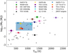 |
Fig. 1 Known gas giants and JWST targets. The blue shaded area represents the approximate parameter space of warm Saturns. Several often studied exoplanets are shown. |
2 Approach
The step-wise iterative process applied in this study was initiated by 3D GCM simulations of the temperature, gas, densities, and wind velocities (Sect. 2.1). 1D profiles were extracted from this 3D atmosphere solution and used as input for a kinetic cloud formation model and the local cloud opacities were calculated (Sect. 2.2). The cloud opacity structure was then used as input for the 3D GCM, and a new atmosphere structure was calculated. Each of the models was executed in its full complexity. This iteration is possible because the cloud formation timescales are considerably shorter than the hydrodynamic timescales (Helling et al. 2001; Helling & Woitke 2006; Powell et al. 2018; Kiefer et al. 2024). The stopping criterion for the iteration is described in Sect. 2.3. In order to explore how the iterative processes may affect the spectral information, transmission spectra were created for each iteration. This was done by first modelling the non-equilibrium gas-phase chemistry of H/C/N/O species based on the final output from each GCM run (Sect. 2.4). The resulting relative concentrations of the gas species were then used to calculate the transmission spectra for each iteration, and we assessed the JWST’s observability of the differences (Sect. 2.5).
2.1 3D atmosphere
The 3D temperature and horizontal (zonal and meridional) wind velocities in the atmosphere of HATS-6b were simulated with the non-grey 3D GCM expeRT/MITgcm (Schneider et al. 2022c; Carone et al. 2020). This model solves the hydrostatic primitive equations (HPE) in vertical pressure coordinates on a rotating sphere (see, e.g. Showman et al. 2009). Hydrostatic equilibrium and the ideal gas law as equation of state are assumed. The model uses the dynamical core of MITgcm (Adcroft et al. 2004), which solves the HPE on an Arakawa C-type cubed-sphere grid. We employed the nominal horizontal resolution C321, a vertical grid with 41 logarithmically spaced grid cells between 1 × 10⁻⁵ bar and 100 bar, and six linearly spaced grid cells between 100 bar and 700 bar. expeRT/MITgcm couples the dynamical core of the MITgcm (Adcroft et al. 2004) to the radiative transfer solver of petitRADTRANS (Mollière et al. 2019). The model includes Rayleigh friction at the top (at 10−5 bar) and bottom (at 700 bar) of the computational domain in order to stabilise the atmosphere against unphysical gravity waves and to mimic Ohmic dissipation (Carone et al. 2020).
We used a stellar effective temperature and stellar radius of HATS-6 of 3724 K and 0.57 R⊙, and we assumed HATS-6b to be tidally locked on a circular orbit with an orbital separation and period of 0.03623 AU and 3.3252725 days. The surface gravity was assumed to be 7.94 ms−2, and the internal temperature was set to Tint = 50 K following Thorngren et al. (2019).
The thermal forcing part of expeRT/MITgcm solves the radiative transfer equation including isotropic scattering using the Feautrier method (Feautrier 1964) with approximate lambda iteration (Olson et al. 1986). expeRT/MITgcm uses 11 correlated-k wavelength bins for the radiative transfer calculations (S1 resolution; Schneider et al. 2022c). We chose to use a radiative time-step of 100 s, which is four times the dynamical time-step2. GGChem (Woitke et al. 2018) was used to pre-calculate a grid of chemical equilibrium abundances that were then used to generate a premixed opacity grid for expeRT/MITgcm. The elemental abundances were assumed solar (Asplund et al. 2009) with a solar C/O ratio of C/O = 0.54 and scaled for the metalicity of HATS-6b of [Fe/H] = 0.2 ± 0.09 (Hartman et al. 2015). A gas temperature Tgas and gas pressure pgas grid for 100–10 000 K, 10−5−650 bar was calculated. Taking the temperature and pressure averages from this premixed grid, we obtained the specific gas constant R = 3925 J kg−1 K−1 and specific heat capacity at constant pressure of cp = 14966 J K−1.
Most absorption cross sections were obtained from exomol3. The H2O, CO2, CH4, NH3, CO, H2S, HCN, PH3, TiO, VO, FeH, Na, and K opacities were used for the gas absorbers4. Furthermore, we included Rayleigh scattering with H2 (Dalgarno & Williams 1962) and He (Chan & Dalgarno 1965) and collisioninduced absorption (CIA) with H2−H2 and H2−He (Borysow et al. 1988, 1989; Borysow & Frommhold 1989; Borysow et al. 2001; Richard et al. 2012; Borysow 2002) and H− (Gray 2008).
2.2 Cloud structure
The results from expeRT/MITgcm were used as input to a kinetic cloud formation model. 1D (Tgas(z), pgas(z), vz(z)) profiles were extracted for each point in a longitudelatitude grid, with a spacing of 45° in longitude (ϕ = {−135°, −90°, −45°, 0°, 45°, 90°, 135°, 180°}) and ~22.5° in latitude (θ = {0°, 23°, 45°, 68°, 86°}), similar to previous works (Helling et al. 2016, 2019a,b, 2020, 2021; Samra et al. 2022; Carone et al. 2023; Helling et al. 2023). Tgas(z) [K] is the local gas temperature, pgas(z) [bar] is the local gas pressure, and vz(z) [cm s−1] is the local vertical velocity component of the 1D profile extracted from the 3D GCM. Each 1D model was run top-down in the atmosphere until it reached at least 0.1 bar. For the southern hemisphere (θ < 0°), all grid points were mirrored across the equator (θ = 0°). GGChem was used to determine the local gas-phase composition in chemical equilibrium for which solar elemental abundances from Asplund et al. (2009) were initially assumed, which are scaled for the metallicity of HATS-6b.
2.2.1 Cloud formation
Our kinetic cloud formation model treats the micro-physical processes of nucleation, bulk growth, and evaporation in combination with gravitational settling, element consumption, and replenishment using the moment method for the moments Lj(V) in volume space V (Gail & Sedlmayr 1986, 1988; Dominik et al. 1993; Woitke & Helling 2003, 2004; Helling et al. 2004; Helling & Woitke 2006; Helling et al. 2008b). Cloud condensation nucleii (CCNs) are considered to form from four nucleating species: TiO2, SiO, KCl, and NaCl. This choice was based on the nuclei included in previous studies (Lee et al. 2015; Bromley et al. 2016; Lee et al. 2018; Gao & Benneke 2018; Köhn et al. 2021; Sindel et al. 2022; Kiefer et al. 2023). However, we note that there are current efforts to expand the list of nucleating species (e.g. Gobrecht et al. 2022, 2023; Lecoq-Molinos et al. 2024). The growth of the mixed-material cloud particles was modelled through the surface growth of 16 bulk materials: TiO2[s], Mg2SiO4[s], MgSiO3[s], MgO[s], SiO[s], SiO2[s], Fe[s], FeO[s], FeS[s], Fe2O3[s], Fe2SiO4[s], Al2O3[s], CaTiO3[s], CaSiO3[s], KCl[s], and NaCl[s]. These materials grow and evaporate through 132 surface reactions (Helling et al. 2019a) onto the surface of the CCN. The formation and evaporation of cloud particles depletes and replenishes the 11 participating elements Mg, Si, Ti, O, Fe, Al, Ca, S, Na, K and Cl, which affects the gas-phase equilibrium abundances. The kinetic cloud model assumes a cloud-free element reservoir deep in the planet. Through mixing, the upper layers are replenished with cloud-forming elements. The exact strength of the mixing within exoplanet atmospheres is difficult to determine (Parmentier et al. 2013; Steinrueck et al. 2019; Samra et al. 2022). For this study, we used a quasi-diffusive approach using the standard deviation of neighbouring cells to compute a relaxation timescale (see Appendix B in Helling et al. 2023). Previous work (e.g. Gao et al. 2020) considered sulfur-, manganese-, and zinc-bearing species, which typically condense below 1000 K for pressure ranges between 10−4 bar to 102 bar. However, these elements are much less abundant and therefore do not contribute significantly to the composition of cloud particle material.
The resulting volume fractions Vs/Vtot og the cloud material, where Vs is the cloud particle volume of a given species s and Vtot is the total cloud particle volume, the average particle size ⟨a⟩ [cm], and the cloud particle number density nd [cm−3] were provided as input for the opacity calculation in the 3D GCM. All cloud particles were assumed to be spherical.
2.2.2 Treating cloud formation mixing
Since our cloud model calculates the cloud structure in the stationary case, the elemental replenishment has to balance the depletion through nucleation, bulk growth, and gravitational settling (Woitke & Helling 2004). For each atmospheric layer, the rate at which elements are replenished from the deep atmosphere is described by the mixing timescale τmix. This timescale is calculated using the vertical velocities extracted from the GCM as described in Appendix B in Helling et al. (2023). Consistent with our cloud formation model, the mixing timescale is therefore derived locally and is not constant throughout the atmosphere (Helling et al. 2019b, 2021). Replenishment is also sometimes described as a diffusive process that is common for chemical kinetics models, where the diffusion coefficient is called Kzz (e.g. Moses et al. 2011; Agundez et al. 2014; Tsai et al. 2017; Baeyens et al. 2021; Konings et al. 2022). Other studies have used Kzz to derive a replenishment timescale through ![Mathematical equation: $\[\tau_{\text {dif }} \sim H_{p}^{2} / K_{\mathrm{zz}}]$](/articles/aa/full_html/2024/12/aa50753-24/aa50753-24-eq1.png) , where Hp [cm] is the scale height (see e.g. Charnay et al. 2018; Helling et al. 2019a). The difference between τdif and τmix is that τdif describes the exchange between adjacent atmospheric layers, whereas τmix describes the rate at which elements are replenished from the deep atmosphere through convective processes to a given atmospheric layer.
, where Hp [cm] is the scale height (see e.g. Charnay et al. 2018; Helling et al. 2019a). The difference between τdif and τmix is that τdif describes the exchange between adjacent atmospheric layers, whereas τmix describes the rate at which elements are replenished from the deep atmosphere through convective processes to a given atmospheric layer.
A hallmark of the climate of close-in tidally locked gas giants is a strong equatorial wind jet (Showman & Polvani 2011). The high hydrodynamic velocities lead to advection timescales that are typically shorter by orders of magnitude than the gravitational settling or diffusion of cloud particles (Woitke & Helling 2003; Powell & Zhang 2024). The nucleation and bulk growth timescales of cloud particles, on the other hand, can still be shorter than the advection timescales (Helling & Woitke 2006; Lee et al. 2018; Powell & Zhang 2024; Kiefer et al. 2024). Studies that considered the horizontal transport of cloud particles (e.g. Lee et al. 2016; Lines et al. 2018b; Komacek et al. 2022; Lee 2023; Powell & Zhang 2024) suggested that the number density and size of cloud particles are more longitudinally uniform than studies that only considered vertical mixing as the cloud particle transport mechanism (e.g. Helling et al. 2021; Roman et al. 2021; Samra et al. 2022; Helling et al. 2023). Similarly, gas-phase species be replenished through both horizontal and vertical mixing. Which of the two dominates depends on the atmospheric conditions. Studies comparing vertical and horizontal mixing timescales for gas-phase species found that at pressures below 0.1 bar, vertical mixing often dominates (Helling et al. 2019b; Baeyens 2021; Zamyatina et al. 2024). In general, it is computationally expensive to consider the horizontal transport of cloud particles. Studies evaluating the effect of horizontal transport were either limited to few simulation days (e.g. Lee et al. 2016; Lines et al. 2018b), made simplifying assumptions about the cloud formation (e.g. Komacek et al. 2022; Roman et al. 2021; Lee 2023), or made simplifying assumptions about the horizontal transport (e.g. Powell & Zhang 2024).
2.2.3 Numerical aspects of the cloud-GCM interface
The 3D GCM employs a sponge layer to stabilise the upper boundary, and it employs basal Rayleigh drag to stabilise the lower boundary. While both layers ensure numerical stability, they are also physically justified.
The cloud model that interfaces with the GCM, similarly, requires numerical stabilisation measures that are justified by physical mechanisms that limit the condensate cloud model. At the upper boundary of the modelling domain, the growth of the cloud particles is limited by decreasing collisional rates in the upper atmosphere. At the lower boundary, cloud growth is limited by the evaporation of cloud materials in the dense and hot deeper atmosphere. To ensure numerical stability, the cloud particle opacities were decreased linearly at the upper and lower pressure limit of the expeRT/MITgcm pressure grid until they reached zero. This decrease prevented a sudden drop in opacities that would otherwise trigger instabilities in the radiative transfer. At the top of the atmosphere, the cloud structure was only interpolated in the uppermost grid cell at p = 10−5 bar. At the high-pressure limit of the cloud structures, the interpolation started from the the lowest pressure of the cloud structure, which is at pressures higher than 10−1 bar.
The expeRT/MITgcm uses a cubed-sphere C32 grid (Adcroft et al. 2004). The cells of this grid are more uniformly distributed than a longitude-latitude grid, which prevents overcrowding at the poles. The resolution of each cell in the C32 grid is approximately 2.8 by 2.8 degrees. The interpolation from the low-resolution longitude-latitude cloud model grids to the expeRT/MITgcm cubed-sphere grid was made using two interpolation steps to reduce interpolation artefacts while keeping the structure of the low-resolution grid. First, a bilinear interpolation to a longitude-latitude grid with cell size Δlon = Δlat = 3 degrees was performed. Afterwards, a bilinear interpolation to a cubed-sphere grid was used. During runtime, clouds were added incrementally to prevent sharp changes in the opacity structure. Out of the 2000 total simulation days, the first 100 simulation days were run without clouds. Then, cloud opacities were linearly increased over the next 100 simulation days until they were fully added at simulation day 200.
The step-wise iterative process applied here is a hands-on version of the iteration processes executed in every complex model implemented as, for example, an operator splitting method in Helling et al. (2001). These methods make use of the timescale difference that may occur, for example, between condensation and hydrodynamical processes. In the case of cloud formation, the formation processes modelled here (nucleation, growth, and evaporation) act on very short timescales because they predominantly occur in collisionally dominated gases in exoplanet atmospheres. This may change in the upper atmosphere regions between 10−4 − 10−5 bar, however, where the densities are so low that photochemistry, for instance, affects the gas phase. We took photochemistry into account in the post-processing. The majority of the cloud formation occurs at deeper levels and, cloud haze models that extend higher up (Steinrueck et al. 2021) still find that the hydrodynamic assumption for these layers is adequate. Further, we aimed to resolve the atmosphere regions that are accessible in the infrared by JWST, which are typically at pressures higher than 10−4 bar.
Possible long-term changes of the thermodynamic atmosphere structure may be linked to the deep atmosphere, which can take more than 80 000 simulation days to converge (Wang & Wordsworth 2020; Schneider et al. 2022b). Similarly, 1D timedependent cloud models have shown that convergence times can reach up to 8000 simulation days (Woitke et al. 2020). Fully coupled cloudy GCMs are computationally intensive and therefore often limited to evaluation times shorter than 5000 simulation days (e.g. Lee et al. 2016, 2017; Roman & Rauscher 2017, 2019; Lines et al. 2018a,b; Roman et al. 2021; Komacek et al. 2022). However, recent run-time improvements of GCMs (Schneider et al. 2022c) might allow for longer simulation times in the future. It should be noted, however, that we obtained only a minor change in the upper atmosphere structure (p < 1 bar) after 2000 days of simulation time (see Appendix C).
2.2.4 Cloud opacities
To calculate the interaction between the photons and the cloud particle, we used the Mie-theory (Mie 1908). This theory is an analytical solution of the Maxwell equations under the assumption of a spherical particle with an effective refractive index εeff.
To find the effective refractive index εeff of a given mixture of bulk material, we followed the approach of Lee et al. (2016) and started by using the Bruggeman mixing rule (Bruggeman 1935). In case of non-convergence, we used the Landau-Lifshitz-Looyenga method (Looyenga 1965). The homogeneous opacity values for all species s used in this paper can be found in Appendix B. Using the effective refractive index, we use Mie-theory to calculate the absorption efficiency Qabs, the scattering efficiency Qsca and the anisotropy factor g. From these, the wavelength-dependent absorption coefficient ![Mathematical equation: $\[K_{\mathrm{abs}}^{\text {cloud}}(\lambda)\left[\mathrm{cm}^{2} \mathrm{~kg}^{-1}\right]\]$](/articles/aa/full_html/2024/12/aa50753-24/aa50753-24-eq2.png) and the scattering coefficient
and the scattering coefficient ![Mathematical equation: $\[\kappa_{\mathrm{sca}}^{\text {cloud}}(\lambda) \left[\mathrm{cm}^{2} \mathrm{~kg}^{-1}\right]\]$](/articles/aa/full_html/2024/12/aa50753-24/aa50753-24-eq3.png) were calculated:
were calculated:
![Mathematical equation: $\[\kappa_{\mathrm{abs}}^{\text {cloud }}(\lambda)=\pi\langle a\rangle^{2} \frac{n_{\mathrm{d}}}{\rho_{\mathrm{gas}}} ~Q_{\mathrm{abs}}\left(\langle a\rangle, \lambda, \epsilon_{\mathrm{eff}}\right)\]$](/articles/aa/full_html/2024/12/aa50753-24/aa50753-24-eq4.png) (1)
(1)
![Mathematical equation: $\[\kappa_{\mathrm{sca}}^{\mathrm{cloud}}(\lambda)=\pi\langle a\rangle^{2} \frac{n_{\mathrm{d}}}{\rho_{\mathrm{gas}}} ~Q_{\mathrm{sca}}\left(\langle a\rangle, \lambda, \epsilon_{\mathrm{eff}}\right)(1-g)\]$](/articles/aa/full_html/2024/12/aa50753-24/aa50753-24-eq5.png) (2)
(2)
where nd [cm−3] is the number density of cloud particles, ⟨a⟩ [cm] is the mean cloud particle radius, ρgas [g cm−3] is the gas density, and λ [cm] is the wavelength of the photon. Our cloud model uses the moment method, which allowed us to efficiently model heterogeneous cloud particles without an explicit size distribution of the cloud particles. If the full size distribution of cloud particles were to be reproduced (Helling et al. 2008b), a functional form would be required. We therefore assumed monodisperse cloud particles with a local mean particle size derived from the kinetic cloud model as used in Helling et al. (2020). The effect of the assumptions of monodisperse cloud particles was studied by Samra et al. (2020). The absorption and scattering coefficients were then added to the gas-phase opacities of the radiative transfer of expeRT/MITgcm,
![Mathematical equation: $\[\kappa_{\mathrm{abs}}^{\text {tot}}(\lambda)=\kappa_{\mathrm{abs}}^{\mathrm{gas}}(\lambda)+\kappa_{\mathrm{abs}}^{\text {cloud}}(\lambda)\]$](/articles/aa/full_html/2024/12/aa50753-24/aa50753-24-eq6.png) (3)
(3)
![Mathematical equation: $\[\kappa_{\mathrm{sca}}^{\mathrm{tot}}(\lambda)=\kappa_{\mathrm{sca}}^{\mathrm{gas}}(\lambda)+\kappa_{\mathrm{sca}}^{\mathrm{cloud}}(\lambda)\]$](/articles/aa/full_html/2024/12/aa50753-24/aa50753-24-eq7.png) (4)
(4)
where ![Mathematical equation: $\[\kappa_{\mathrm{abs}}^{\mathrm{gas}}\left[\mathrm{m}^{2} \mathrm{~kg}^{-1}\right]\]$](/articles/aa/full_html/2024/12/aa50753-24/aa50753-24-eq8.png) and
and ![Mathematical equation: $\[\kappa_{\mathrm{sca}}^{\mathrm{gas}}\left[\mathrm{m}^{2} \mathrm{~kg}^{-1}\right]\]$](/articles/aa/full_html/2024/12/aa50753-24/aa50753-24-eq9.png) are the absorption and scattering coefficients for the gas, respectively.
are the absorption and scattering coefficients for the gas, respectively. ![Mathematical equation: $\[\kappa_{\text {abs}}^{\text {tot}}\left[\mathrm{m}^{2} \mathrm{~kg}^{-1}\right]\]$](/articles/aa/full_html/2024/12/aa50753-24/aa50753-24-eq10.png) and
and ![Mathematical equation: $\[\kappa_{\mathrm{sca}}^{\mathrm{tot}}\left[\mathrm{m}^{2} \mathrm{~kg}^{-1}\right]\]$](/articles/aa/full_html/2024/12/aa50753-24/aa50753-24-eq11.png) are the total absorption and scattering coefficients, respectively.
are the total absorption and scattering coefficients, respectively.
2.3 Stopping the step-wise iteration
One of the aims of this work is to demonstrate that a 3D atmosphere solution including detailed cloud formation is computationally feasible for warm Saturn-type exoplanets. We demonstrate this through a step-wise iteration between the two modelling complexes. This enables the full complexity of both the 3D GCM and the cloud model, to achieve a conceivable accuracy for a global exoplanet atmosphere structure.
We determined the conceivable accuracy from the observational accuracy, and the stopping criterion therefore depends on the observational facilities used. For this project, the spectral precision of transmission spectra from the JWST instruments NIRspec Prism and MIRI LRS after two and after ten transit measurements were used as the primary stopping criterion. After each iteration, a transmission spectrum was calculated (Sect. 2.5) and compared to the previous iteration step. When the observational differences between iterations fell below the spectral precision, the step-wise iteration was stopped. Since our model iterates between the cloud model and the GCM, the main goal was to have no observable impact of the changing cloud structure on the transmission spectra. The abundances in chemical disequilibrium were calculated in post-processing, and the impact on the transmission spectra was used as a secondary stopping criterion.
Additional further stopping criteria may be derived from the structures of (Tgas, pgas) and the cloud opacity. As we demonstrated below, when the changes in the transmission spectra fall below the observable accuracy, the cloud properties between the two successive iterations remain similar. This suggests that the still existing changes between the structures of (Tgas, pgas), which may be substantial but locally confined, do not affect the structure of the gas phase and cloud opacity sufficiently enough to change the spectrum beyond the spectral precision. Hence, these changes do not affect the interpretation of the data.
2.4 Disequilibrium gas-phase chemistry
The disequilibrium chemistry for the H/C/N/O complex of HATS-6b was modelled to assess how each iteration affects the atmospheric chemistry, and as a result the transmission spectra. This was done using an updated version of the chemical network STAND2020 (Rimmer & Helling 2016, 2019; Rimmer & Rugheimer 2019) in combination with the 1D photochemistry and diffusion code ARGO (Rimmer & Helling 2016). ARGO models chemical transport, wavelength-dependent photochemistry, and cosmic-ray transport by following a parcel of gas as eddy diffusion leads it up and down through the atmosphere (further description in e.g. Rimmer & Helling (2016) and Barth et al. (2021)). STAND2020 is a chemical H/C/N/O network containing the reaction rates for more than 6600 reactions in the temperature range of 100 K to 30000 K. STAND2020 involves all reactions for species containing up to six H, two C, two N, and three O atoms and also contains reactions with He-, Na-, Mg-, Si-, Cl-, Ar-, K-, Ti-, and Fe-bearing species. The network was tested for the atmospheres of Earth and Jupiter (Rimmer & Helling 2016) and on a number of hot-Jupiter models (Barth et al. 2021; Hobbs et al. 2021; Tsai et al. 2023). The chemical network was run through the 1D photochemistry and diffusion code, ARGO, which modeled the chemical transport and the effect of photochemistry and cosmic rays.
The inputs for ARGO and STAND2020 were chosen as described below:
(Tgas, pgas) profiles and vertical eddy diffusion profile: Eight different 1D profiles were extracted from the output of the expeRT/MITgcm by averaging over areas of the 3D grid. The eight profiles are six terminator regions with the longitudes (ϕ = {90°, 270°}) and latitudes (θ = {0°, 23°, 68°}), and the sub-stellar and anti-stellar points.
Atmospheric element abundances: Solar abundances were adapted for metallicity ([Fe/H] = 0.2) in accordance with the initial abundances used for the GCM.
Stellar XUV (X-ray and ultra violet) spectrum driving photochemistry: We obtained a spectrum from the MUSCLES (Measurements of the Ultraviolet Spectral Characteristics of Low-mass Exoplanetary Systems) survey where the M1.5V star, GJ667C, was chosen as a proxy for HATS6. The spectrum covers the XUV range and is composed of a combination of modelled and observed spectra (France et al. 2016; Youngblood et al. 2016, 2017; Loyd et al. 2016, 2018). The XUV spectrum used in this study is shown in Appendix D.1.
Cosmic rays: We implemented cosmic rays based on the ionisation rate of low-energy cosmic rays (LECR) as explained by Rimmer & Helling (2013) and Barth et al. (2021).
Stellar energetic particles (SEP): To account for the higher activity of M dwarf host stars, SEPs were included in the model. The SEPs were introduced by scaling the spectrum of a solar SEP event to fit the host star based on the X-ray flare intensity (method further described in Barth et al. 2021). A number of X-ray flare intensities has been reported for M dwarf stars (Hünsch et al. 2003; Namekata et al. 2020). They range from ~ 0.001 to 0.2 W m−2 at 1 AU. We chose to implement SEPs corresponding to X-ray flare intensities of 0.1 W m−2 at 1 AU. The effect of the SEPs was included continuously throughout the run, and not as a finite event.
Different locations on the planet will experience a different influx of stellar radiation and SEPs, and the model inputs were therefore varied accordingly. For the sub-stellar point, both the stellar spectrum and SEPs were included. For the anti-stellar point, neither the stellar spectrum nor SEPs were included. For the terminator coordinates, only SEPs were included. We included SEPs but not the stellar spectrum for the terminator region because the shallow angle of incidence for radiation from the host star causes the radiation to pass through so much atmospheric layers before it reaches the bulk of the 1D simulated atmosphere profile above the terminator that its influence is negligible. Since XUV radiation is easily scattered by the atmosphere, the stellar spectrum was not included for the terminator regions, whereas SEPs have been shown to penetrate deeper into the atmosphere (Barth et al. 2021) and were therefore included. The SEPs were not scaled based on the incident angle. The output of the STAND2020-ARGO run is the relative concentrations (ni/ngas) of more than 511 gas-phase species. Based on these relative concentrations as well and on the cloud opacities mentioned previously, the transmission spectra can be produced.
2.5 Transmission radiative transfer
The transmission spectrum of HATS-6b was produced by adding the cloud opacities to petitRADTRANS (Mollière et al. 2019, 2020; Alei et al. 2022), where the cloud opacities from the micro-pyhsical cloud model were included as opacity source (Sect. 2.2.4). Each transmission spectrum used the input cloud structure for the GCM, the temperature structure of the GCM, and the post-processed gas-phase relative concentrations from ARGO. The transmission spectrum of the cloudless GCM run (iteration 0) was calculated cloud free.
To calculate the transmission spectrum, we divided the terminator region into ten equally spaced and equally sized grid cells. Each cell covered a latitudinal range of Δlat = 22.5°. A constant longitudinal range would lead to the neglect of data points within the terminator region, especially, close to the poles. Therefore, a latitude-dependent longitudinal range was chosen to ensure equally sized grid cells. At the equator, the longitudinal range was ±Δlon = 10° (Lacy & Burrows 2020). The total transmission spectrum was then calculated as the average of the transmission spectra from all regions,
![Mathematical equation: $\[R_{\mathrm{tot}}(\lambda)=\sqrt{\frac{1}{N} \sum_{i=1}^{N} R_{i}^{2}(\lambda)}.\]$](/articles/aa/full_html/2024/12/aa50753-24/aa50753-24-eq12.png) (5)
(5)
Similar to previous studies (Lee et al. 2019; Baeyens et al. 2021; Nixon & Madhusudhan 2022), the following gas-phase species were considered as line opacity species5: H2O, CO, CH4, CO2, C2H2, OH, NH3, and HCN. Furthermore, H2 and He were considered as Rayleigh-scattering opacities, and collision-induced absorption (CIA) from H2−H2 and H2−He was included.
3 Evaluation of the combined model
To study the atmosphere of the warm-Saturn HATS-6b, six iterations using expeRT/MITgcm and the kinetic cloud model were conducted. After each iteration of the GCM, the thermodynamic structure was used to produce a cloud-structure that was included in the next iteration of the GCM. The cloud-free simulations are shown in Sect. 3.1. The effect of clouds is presented in Sect. 3.2. After each GCM run, the disequilibrium chemistry (Sect. 3.3) was post-processed and the differences in the transmission spectrum were determined (Sect. 3.4).
3.1 Cloud-free GCM and post-processed clouds
The first run, that is, iteration 0, of the GCM was conducted without clouds. A total of 2000 days were simulated using expeRT/MITgcm. After 2000 days, there was little change in the global average of the (Tgas, pgas) profiles for pressure layers lower than 1 bar (see Appendix C). For pressures higher than 1 bar, the temperature did not change by more than 20 K from the initial conditions for the GCM. It is well known, that the convergence deeper in the atmosphere is computationally intensive and difficult to achieve (Wang & Wordsworth 2020; Skinner & Cho 2022; Schneider et al. 2022c,b). In the cloudy iterations (see Sect. 3.2), the clouds become opaque for pressures higher than 10−2 bar. Therefore, the atmospheric layers of interest for this study can be assumed to be reasonably converged.
The (Tgas, pgas) profiles for the sub-stellar point, anti-stellar point, morning terminator, and evening terminator are shown in Fig. 2. The iteration 0 profiles only show minor differences in temperature for pressures greater than 10−1 bar. Higher up in the atmosphere, the dayside is roughly 200 K hotter than the nightside. The isobaric temperature maps for p = 1.2 × 10⁻³ bar and p = 1.2 × 10⁻² bar are shown in the left panels of Fig. 3. The zonal mean wind velocities are shown in the left panel of Fig. 4, which describes the longitudinal average of winds parallel to the equator. These winds are known to redistribute heat longitudinally (Vuitton 2021). Overall, the global temperature and wind velocity structure of HATS-6b show the characteristics of a highly irradiated gas giant including a super-rotating equatorial jet stream. This jet stream transports heat from the day- to the nightside and causes a hot-spot offset (e.g. Showman & Polvani 2011; Cowan et al. 2012; Dang et al. 2018). In addition to the equatorial jet stream, two weak polar jet streams can be observed.
Using the output from the cloudless GCM (iteration 0), we postprocessed the cloud structure. This cloud structure is labelled iteration 1 because we used it later as input for the first cloudy iteration of the GCM (iteration 1). The iteration 1 cloud profile of HATS-6b shows global cloud coverage. In Fig. 5, the nucleation rate J⋆, cloud particle number density nd, average cloud particle size ⟨a⟩, and cloud mass fraction6 ρd/ρ are shown for the morning and evening terminator. The sub-stellar and anti-stellar point are shown in Fig. A.1. The cloud particle properties of these profiles are largely the same, although there is an increase in the nucleation rate for the upper atmosphere (p < 10−3 bar) for the cooler profiles (morning terminator and anti-stellar point) with a corresponding increases in cloud particle number density and cloud mass fraction for these points. The cloud condensation nuclei (CCNs) predominantly form in the upper atmosphere (p < 10−2), but we note that condensation still occurs in these upper regions – hence, the increase in average particle size. In deeper layers, the cloud particle sizes steadily increase while the cloud particle number densities steadily decrease. This inverse correlation between cloud particle number density and cloud particle size is well known (see Helling et al. 2021). When more cloud particles are present, the same mass of condensation material is spread out over more particles, which reduces the average size of the particles.
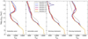 |
Fig. 2 (Tgas, pgas) profiles of the sub-stellar point, anti-stellar point, evening terminator, and morning terminator. |
3.2 Impact of clouds on the atmospheric structure
Iterations 1, 2, 3, 4, and 5 of the GCM were created by including the post-processed cloud opacities from the previous iteration into expeRT/MITgcm as described in Sect. 2.2. The GCM was again run for 2000 simulation days. Similar to iteration 0, there was little change in the global average temperature above 1 bar after 2000 simulation days (see Appendix C).
The differences from iteration 0 to iteration 1 highlight the impact of clouds on the temperature and wind structure due to the increased local opacities. The most striking difference is a strong temperature inversion for pressures lower than 10−2 bar (higher altitudes) on the sub-stellar point and the evening terminator (Fig. 2). This increased temperature is also visible in the isobaric plots (Fig. 3). At pressures between 10−2 bar and 10 bar, the (Tgas, pgas) profiles of iteration 1 show a considerably colder temperature. This drop can be explained with an anti-greenhouse effect (see Sect. 5.1). For pressures higher than 10 bar, no significant differences in the (Tgas, pgas) profiles were found. Furthermore, iteration 1 has a stronger and narrower equatorial wind jet than iteration 0 (see left panel of Fig. 4). This matches the results of Baeyens et al. (2021), who showed that for the temperature range of warm Saturns (500 K to 1200 K) an increase in equilibrium temperature results in a faster and narrower jet. The cloud-induced temperature inversion seems to have a similar effect. Furthermore, the weak polar jets of iteration 0 are not observed in iteration 1.
Fewer differences are observed from iteration 1 to iteration 2 in the thermal and wind structure of HATS-6b than from iteration 0 to 1. However, the temperature profile still changes by up to 90 K. The exception to this is the morning terminator around 10−4 bar, where a temperature increase of up to 350 K can be seen. This increase in temperature also reduces the nucleation rate, which in turn leads to fewer but larger particles (Fig. 5). The sudden change in the morning terminator is caused by a dynamical instability caused by the cloud structure of iteration 2, which leads to hot air being advected from the dayside into the morning terminator. The general thermal instabilities of the morning terminator are discussed in more detail in Sect. 5.2. While an instability is present in all cloudy iterations, it is more pronounced in iteration 2. The persistence of this instability is a result of the static cloud structures. Since no other iteration shows a similar behaviour, the temperature increase in the morning terminator of iteration 2 was considered an artefact of the specific configurations of the static clouds.
Iterations 3, 4, and 5 all show the same general characteristics as iterations 1 and 2: a temperature inversion around 10−3 bar, a cooling around 0.1 bar to 1 bar, a narrow equatorial wind jet, and global cloud coverage. However, the temperature between iterations after iteration 2 still varies by up to ~130 K. Similarly, differences in the temperature structure around 10−3 bar can be seen in the isobaric plots (Fig. 3) and in the zonal mean winds (Fig. 4). The cloud particle properties, on the other hand, vary little between iterations 3, 4, and 5. In particular, the nucleation rate between iterations 4 and 5 is close to identical. Nevertheless, there are still changes in the cloud particle number density and average size between iterations 4 and 5. As mentioned previously, the goal of this work is to find a solution within the observational accuracy of JWST, and therefore, only observable changes within the atmospheric structure matter. Whether the changes described here have an observable effect is analysed in Sect. 3.4.
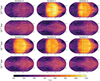 |
Fig. 3 Isobaric slices of the expeRT/MITgcm runs at t = 2000 simulation days. The white lines indicate the horizontal wind velocity fields. |
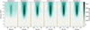 |
Fig. 4 Zonally averaged zonal wind velocities at t = 2000 simulation days. |
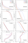 |
Fig. 5 Cloud particle properties of the step-wise iterated cloud structure for the warm Saturn example HATS-6b. Iteration 5 is shown as a solid line to highlight the final result. Left: morning terminator. Right: evening terminator. Top: cloud mass fraction ρd/ρ. Upper middle: cloud particle number density nd. Lower middle: average cloud particle size ⟨a⟩. Bottom: nucleation rate J⋆. The sub- and anti-stellar point are shown in Fig. A.1. |
3.3 Disequilibrium chemistry
To assess the impact of the kinetic gas-phase chemistry and photo-chemistry on the observable atmosphere, and more specifically, on transmission spectra of HATS-6b, the disequilibrium chemistry was modelled for each iteration at six coordinates along the terminator region (longitudes (ϕ = {90°, 270°}) and latitudes (θ = {0°, 23°, 68°})). The resulting gas concentration profiles were averaged over the six coordinates. The relative concentrations ni/ngas of H, H2, CO, CO2, H2O, CH4, HCN, and NH3 are shown in the top panel of Fig. 6. These eight molecules were chosen due to their high concentrations in the atmospheres or because they are some of the more interesting atmospheric species for the effects of external radiation (e.g. Barth et al. 2021; Baeyens et al. 2022). The concentration profiles show very little variation among the five iterations with clouds, whereas the difference between the cloudless (iteration 0) and cloudy iterations (1–5) is somewhat larger. The largest differences between the cloudless and cloudy iterations occurs between pgas ~ 10−2−100 bar (top of Fig. 6). This pressure range corresponds to a cloud-induced cooling, which is present in iterations 1–5. Some species (e.g. NH3, CO2, and CH4) also show a difference between cloudy and cloudless at lower pressures (top panel of Fig. 6) corresponding to a cloudinduced heating in iterations 1–5. The cloud-induced heating in the upper atmosphere in combination with a cooling of the lower atmosphere comprises the temperature inversion (see Fig. 2).
The chemical variations along the equator are illustrated in the middle (sub-stellar and anti-stellar point) and bottom panel (morning and evening terminator). Comparing the top and middle panel we note that the relative concentration of all species shows significantly larger differences between the day- and nightside (the solid and dashed lines in the middle panel) than the differences between the different iterations (all lines in the top panel). We describe the chemistry observed for HATS-6b in more detail in Sect. 4.1.
3.4 Observable differences between iterations
The goal of the step-wise iteration approach was to reach observational accuracy, which we chose to be that of JWST NIRspec and MIRI LRS. For HATS-6b, this was reached after six iterations, that is, after iteration 5.
All transmission spectra were produced using the temperature structure of the GCM and the chemistry of ARGO. The spectrum of the cloudy iterations included the cloud structures as well. All six spectra are shown in the top panel of Fig. 7. The residuals between iterations 1, 2, 3, 4, and 5 are shown in the bottom panel of the same figure. Additionally, the spectral precision for the JWST instruments NIRSpec Prism (Birkmann et al. 2022; Ferruit et al. 2022) and MIRI LRS (Kendrew et al. 2015, 2016) are shown. The spectral precision was calculated using PandExo (Batalha et al. 2017) assuming a spectral resolution7 of R = 10 for two and ten observed transits. When the residuals are significantly higher than the spectral precision, the differences between the iterations are observable. When the residuals are of the same order or lower, it is challenging to observe the differences between iterations.
The transmission spectra of iterations 0 and 1 show clear differences due to the presence of clouds in iteration 1. Compared to iteration 0, the molecular features of iteration 1 are muted for wavelengths below 2 μm. Around 10 μm, an additional increase in the relative transit depth is visible, which is caused by silicate species within the cloud particles. Both these effects are known and expected when clouds are present in exoplanet atmospheres (Wakeford & Sing 2015; Powell et al. 2019; Grant et al. 2023).
The residuals in transit depth from iterations 1 to 2 and 2 to 3 are around 25 ppm for wavelengths between 0.7 μm to 10 μm. This can be related to a shift in the cloud top, which is defined as the pressure level at which clouds become optically thick (see e.g. Estrela et al. 2022). From iteration 3 to iteration 4, the transit depth differs by roughly 30 ppm for wavelengths between 0.7 μm to 10 μm. For the wavelength range of MIRI LRS, the differences between iterations is always below the spectral accuracy even when ten transits were observed. From iterations 4 to 5, the cloud top changed again, but by less than 25 ppm. The residuals between iteration 4 to iteration 5 are now consistently below the spectral precision of NIRSpec Prism, as illustrated by the black data points. The only exception to this are the CH4 features around 2 μm to 4 μm, whose residuals are still around 30 ppm. Since the differences between the transmission spectra of iterations 3,4, and 5 are close to or below the spectral precision of the JWST NIRSpec Prism, we stopped our iterative procedure after iteration 5.
Furthermore, the comparison of the the residuals to the differences between the morning and evening terminator (see Fig. 9) showed that the differences between the limbs are generally larger than the residuals between iterations 4 an 5. This holds true for the cloud continuum (limb ~250 ppm versus residuals <30 ppm), the methane features (limbs ~200 ppm versus residuals <40 ppm), and the water features (limb ~100 ppm versus residuals ~30 ppm).
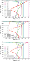 |
Fig. 6 Concentrations of non-equilibrium gas species for the warm Saturn example HATS-6b. Top: terminator region (both morning and evening) averaged over all six coordinates for all iterations. Middle: sub- and anti-stellar point for the final iteration (Iteration 5). Bottom: morning and evening terminators for the final iteration (Iteration 5). |
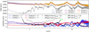 |
Fig. 7 Comparison of the transmission spectra for the warm Saturn example HATS-6b for λ = 0.3 μm to 25 μm Top: transmission spectrum for each iteration. Bottom: absolute residuals between subsequent iterations and the spectral precision for JWST observations with NIRspec Prism and MIRI LRS for two and ten transits. |
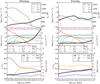 |
Fig. 8 Cloud structure of the morning (left) and evening (right) terminator of HATS-6b. Top: gas temperature Tgas and total J⋆ and JTiO2, and JSiO. Middle: gas-phase relative concentrations ni/ngas and cloud mass fraction ρd/ρ. Bottom: cloud particle volume fractions Vs/Vtot and mean cloud particle size ⟨a⟩. Salts are a minor component and have a volume fraction close to 0. |
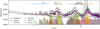 |
Fig. 9 Transmission spectra for the warm Saturn HATS-6b for λ = 0.3 μm to 25 μm including the total spectrum of the final iteration (iteration 5) and the morning and evening terminator separately. We also show the contributions of selected gas-phase species, the contribution of the Si-bearing cloud particle materials, and the spectral accuracy of the JWST instruments NIRSpec prism and MIRI LRS for two and ten transits. |
4 Combined 3D model for the warm Saturn HATS-6b that orbits an M dwarf
The final combined 3D model for the warm Saturn HATS-6b that orbits an M dwarf was demonstrated in Sect. 3. The two isobar maps at pressure ranges that are accessible to transmission spectroscopy are shown in the bottom right panel of Fig. 3 (iteration 5). HATS-6b is affected by a strong equatorial jet that reaches a depth of pgas ≈ 1bar. Horizontally converging flows8 further contribute to the global mixing of the atmosphere in the pole regions (e.g. Baeyens et al. 2021). The temperature inversion is well represented in the upper atmosphere with a temperature difference of ~400K as compared to lower regions, where pgas ≈ 10−2 bar. Sect. 4.1 presents the final results from the combined model, and Sect. 4.2 shows the transmission spectrum as observable with JWST NIRspec prism and MIRI LRS.
4.1 Atmospheric structure of HATS-6b
HATS-6b is a warm Saturn with a hydrogen-dominated atmosphere that we assumed to be oxygen rich. Figure 8 presents the solution of the combined 3D model. The morning (left) and evening (right) 1D terminator profiles were selected to demonstrate the cloud and kinetic chemistry results in enough detail to gain insight into the physical reasons for the differences between the respective transmission spectra that are shown in Sect. 4.2.
Figure 8 (top) shows that the local gas temperatures differ between the morning and evening terminator, which has direct consequences for the cloud formation efficiency. By comparing the nucleation rates (J* [cm−3 s−1]), we note that the cooler morning terminator (left) forms more cloud particles than the hotter evening terminator. Consequently, the mean particle size, ⟨a⟩ [μm], is smaller in the respective low-gas pressure region of the morning terminator. The lower panels in Fig. 8 show the material groups that dominate the cloud particle composition (MO = metal oxides, SC = silicates, HTC = high temperature condensates, or salts), and hence, their opacities. Fig. A.2 contains the detailed breakdown of all 16 modelled bulk materials. Materials that are determined by low-abundance elements such as Cl, Mn etc. can be thermally stable, but appear with ~1% volume contribution (Helling et al. 2017; Woitke et al. 2018).
Figure 8 demonstrates that it is reasonable to expect the cloud particles that form in the atmosphere of a warm Saturn such as HATS-6b to be made of a mix of materials and that their mean particles sizes changes throughout the atmosphere. It further demonstrates that the bulk cloud mass (ρd/ρ, black line, middle panel) is not necessarily equally distributed through the atmospheres and differs between the two terminators. This emphasises the terminator asymmetry. A comparison of the material volume fractions, Vs/Vgas, in the lower panels demonstrates that the bulk mass comes from silicates (MgSiO3[s], Mg2SiO4[s], CaSiO3[s], and Fe2SiO4[s]) and metal oxides (SiO[s], SiO2[s], MgO[s], FeO[s], and Fe2O3[s]) because Mg/Si/Fe/O are the most abundant elements amongst those considered here. The final bulk composition is therefore the result of mass conservation. The high-temperature condensates (TiO2[s], Al2O3[s]) and salts (KCl[s], NaCl[s]) are far less important for the composition of the cloud material, for the same reason. Since most dominant condensation species are oxygen-bearing species and oxygen is far more abundant than Ti, Mg, Si, and Fe, these condensation species do not significantly impact the gas-phase chemistry of non-Ti-, Mg-, Si-, and Fe-bearing species.
As introduced in Sect. 3.3, the disequilibrium chemistry of HATS-6b is shown in Figure 6. The middle and bottom panels show the relative concentrations for a selection of molecular gas species for the last iteration at four coordinates along the equator of the planet: at the sub-stellar point, anti-stellar point, and at the two terminators. The variations along the equator are caused both by differences in the (Tgas, pgas) profiles for the four coordinates and by differences in the stellar XUV radiation and the SEPs. The sub-stellar point is irradiated both by XUV radiation and SEPs, the terminators are irradiated only by SEPs, and the anti-stellar point is irradiated by neither. By comparing the four cases, we show that the sub-stellar point and the two terminators are relatively similar, whereas the anti-stellar point differs significantly from the rest. By comparing the sub- and anti-stellar point, we note a steep decrease in the concentration of many of the gas species at the sub-stellar point (including H2, CH4, and NH3) in the upper atmosphere, indicating a breakdown of these molecules through photolysis by the XUV radiation or ionisation by the SEPs. Other species (e.g. H, HCN, and partly CO and CO2) show an increase in concentration for the sub-stellar point compared to the anti-stellar point farther up in the atmosphere, indicating that these are positively influenced by photochemical reactions. By comparing model runs for the sub-stellar point with and without SEPs (middle panel), we note a significant contribution by the SEPs to the gas-phase concentrations and that this effect reaches far down into the atmosphere. The middle and bottom panels show that the sub-stellar point with SEPs bears a strong resemblance to the terminator regions, which could indicate that SEPs can have a stronger effect than the XUV radiation on the concentrations of the gas species, including observationally interesting species such as CH4 and HCN. The bottom panel shows that the differences between the terminator regions are generally higher at lower pressures, with the exception of H, which also shows differences deeper into the atmosphere.
As mentioned in Sect. 1, M dwarf stars such as HATS-6 are known to have higher magnetic activities than more massive stars like the Sun. This increased activity leads to increased numbers of SEPs. As explained in Sect. 2.4, the numbers of SEPs were found to scale with the X-ray flare intensity of the star, which for M dwarf stars was reported to range from 0.001 to 0.2 W m−2 at 1 AU. We scaled our SEP spectrum based on an X-ray flare intensity of 0.1 W m−2 at 1 AU, indicating that the number of SEPs could be significantly higher than what we show. This would lead to a greater impact on the disequilibrium gas-phase chemistry.
4.2 Transmission spectra
Transmission spectra are used to study the chemical composition and atmospheric asymmetries of gaseous planets. To determine the concentrations of known non-equilibrium species (e.g. CH4 and HCN), we determined the H/C/N/O complex of the gas phase using ARGO (Sect. 3.3). As the methods we used may help us to efficiently interpret the data of JWST and future space missions, the focus was set on spectral features that are relevant for the JWST instruments NIRspec and MIRI. In the following, we present the near-IR transmission spectra that also include non-equilibrium species such as CH4 and HCN for a wavelength range of λ = 0.3 μm to 12 μm.
To create the transmission spectrum of HATS-6b, we used the (Tgas, pgas) profiles from the GCM, the cloud opacities from the kinetic cloud model and the disequilibrium chemistry from ARGO. The full transmission spectra are shown in Fig. 9. We also show the morning and evening spectra separately as well as the cloud and the gas-phase contributions. The transmission spectrum is roughly flat for wavelengths below 2 μm, owing to scattering that is typical for cloudy exoplanets (Bean et al. 2010; Crossfield et al. 2013; Kreidberg et al. 2014; Knutson et al. 2014; Sing et al. 2015, 2016; Benneke et al. 2019). An observation of HATS-6b at these wavelengths would allow us to determine the height of the cloud deck (Mukherjee et al. 2021). Above 3 μm, the gas-phase species start to contribute significantly to the spectrum. Especially CH4 (around 3 μm and 8 μm), H2O (around 6 μm), and HCN (around 10.5 μm) are detected. However, the clouds still strongly mute the spectral features, which makes them harder to detect.
At around 10 μm, the cloud opacities show a broad silicate feature from the Si-bearing cloud particle materials. This feature originates from Si–O vibrations (Wakeford & Sing 2015). A detection this feature could confirm the presence of siliconbearing cloud particle materials in HATS-6b as has been done previously for WASP-17b (Grant et al. 2023) and WASP-107b (Dyrek et al. 2023).
HATS-6b itself may reveal differences in cloud coverage and chemistry between the morning and evening terminator similar to WASP 39b (Carone et al. 2023; Espinoza et al. 2024). The cloud deck is slightly higher at the evening than at the morning terminator, leading to a ~250 ppm offset at short wavelengths (0.3 μm < λ < 2 μm). The observable difference in the gas phase is mainly caused by CH4, which has a ~200 ppm higher signal at the evening terminator than at the morning terminator. H2O has a ~100 ppm higher signal in the evening terminator than the morning terminator. At the morning terminator, the contribution of chemical species to the transmission spectrum can vary strongly with latitude (see Fig. A.3). Especially at ±45° of the morning terminator, stronger transmission features of CH4 and HCN arise as a consequence of the Rossby gyres, which represent particularly cold regions in the atmosphere (see Fig. 3). Warm Saturns and Jupiters in the temperature range between 800 K and 1200 K typically exhibit extended Rossby wave gyres at the morning terminator (e.g. Baeyens et al. 2021, Fig. 2). Thus, a study of morning terminator chemistry in warm Saturns needs to take into account special locations such as the dynamically cool Rossby gyres to correctly infer global atmosphere properties.
5 Discussion
We implemented a 3D climate model in combination with a microphysical cloud model to capture the feedback between the heating, the 3D climate, and cloud formation in its full complexity. The model was applied to the particular example of a warm Saturn around an M dwarf, HATS-6b. Many exoplanet theories predict temperature inversions in exoplanet atmospheres for various reasons. In Sect. 5.1, we discussed the strong cloud-induced temperature inversion of HATS-6b. Furthermore, we discussed the dynamics of the terminators in Sect. 5.2. While several studies modelled the climate and cloud structure of warm Saturns, there have so far been no detailed studies of warm Saturns around M dwarf stars such as HATS-6b. Therefore, we compare in Sect. 5.3 the results for HATS-6b to grid studies including warm Saturns and to detailed models of other Saturn-mass planets similar to HATS-6b.
5.1 Anti-greenhouse effect
The clouds in HATS-6b have considerable cloud particle sizes and number densities for pressures lower than 10−3 bar. The high cloud deck leads to scattering and absorption of the incoming short-wavelength radiation on cloud particles. This reduces the radiative heating of the lower atmospheric layers while simultaneously heating the upper layers. Both effects lead to a temperature inversion in the layers in which clouds are located and a cooling in the layers below. This effect is called the anti-greenhouse effect and was first observed in Titan (McKay et al. 1991). It has also been theoretically predicted for exoplanet atmospheres with either an extended cloud deck or photochemical hazes (Heng et al. 2012; Morley et al. 2012; Steinrueck et al. 2023).
In hotter exoplanets, temperature inversions are not caused by scattering from high-altitude clouds, but by gas-phase species such as TiO and VO (Hubeny et al. 2003; Fortney et al. 2008) or AlO, CaO, NaH, and MgH (Gandhi & Madhusudhan 2019). These species heat the upper atmosphere through the very efficient absorption of stellar radiation in the optical wavelength range. These absorption-driven temperature inversions were observed in (ultra) hot Jupiters (Haynes et al. 2015; Yan et al. 2020, 2022). HATS-6b orbits an M dwarf that emits less flux in the optical wavelength range than a hotter star (Lothringer & Barman 2019). Furthermore, Hu & Ding (2011) predicted that an exoplanet with a CO2-dominated atmosphere orbiting an M dwarf star would also have an anti-greenhouse effect mainly through the highly efficient Rayleigh scattering of CO2 at the top of the atmosphere. In this study, however, CO2 is a minor species, and Rayleigh scattering is dominated by hydrogen and helium. In our simulation of HATS-6b, no temperature inversion is present in the GCM runs without clouds. Therefore, we are confident in our conclusion that the temperature inversion is indeed mainly caused by scattering of stellar irradiation at the top of the extended cloud deck, similar to the anti-greenhouse effect observed in Titan, where it is due to scattering at the top of the atmosphere due to hazes.
For a direct observation of a temperature inversion, emission from the lower atmosphere needs to be observable (Gandhi & Madhusudhan 2019). The strong cloud coverage will likely block all emissions from the lower atmosphere and make direct detections of the temperature inversion unlikely. However, HATS-6b lies in a temperature regime in which quenching is expected to affect the chemistry (e.g. Baeyens et al. 2021). Figs. 7 and 9 show a CH4 feature that is visible despite the cloud layer, which indicates that the CH4 extends into the upper layers of the atmosphere where it is exposed to photolysis and high degrees of SEPs. Since CH4 is very susceptible to photo-chemical reactions (Moses et al. 2011; Line et al. 2011; Baeyens et al. 2021, 2022; Konings et al. 2022), it will most likely break down in the upper atmosphere, and in order to maintain a visible CH4 feature, a constant upwelling from the lower protected part of the atmosphere would be necessary. A visible CH4 feature could therefore indicate that vertical mixing has connected the observable gas-phase chemistry above the clouds to deeper atmosphere layers, thereby forming a probe through the temperature inversion and into the layers cooled by the anti-greenhouse effect (Agundez et al. 2014; Fortney et al. 2020). In addition, we confirmed the influence of stellar energetic particles (SEP) on the dayside chemistry of a planet around a relatively active planet as was already pointed out by Barth et al. (2021) for HD 189733b.
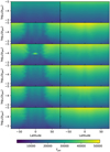 |
Fig. 10 Potential temperature cross section across the morning (left panels) and evening terminators (right panels) for iterations 0 to 5 (from top to bottom). |
5.2 Dynamics of the terminator regions
In Sect. 3, we showed that the morning terminator of iteration 2 develops a temperature spike in the upper atmosphere (see Fig. 2). Since no other iteration shows such a spike, we can conclude that it is caused by the impact of the specific configuration of the static cloud opacities of iteration 2 on the temperature and wind structure of HATS-6b. A closer inspection of the potential temperature profiles across the morning and evening terminators of all iterations (Fig. 10) reveals a potential temperature anomaly at the equator for the morning terminator in iteration 2. The potential temperature is linked to atmospheric stability. If the potential temperature increases monotonically with height, the atmosphere is dynamically stable (e.g. Holton & Hakim 2013).
In the equatorial morning terminator region, the superrotating wind jet advects colder air from the night- to the dayside that is heated by the cloud feedback (see Fig. 3). The advection of cold air results in a minimum in potential temperature between −40 degree and +40 degree latitude. In contrast to this, the potential temperature across the evening terminator is more barotropic. Here, the wind jet broadens and encompasses almost the whole evening terminator region (Fig. 3), resulting in a more uniform advection of warm air towards the nightside.
We wished to identify a stable climate solution for a cloudy warm Saturn orbiting an M dwarf star. However, it may be worthwhile to investigate whether the strong temperature gradients of the morning terminator at the boundary of the super-rotating jet give rise to instabilities and thus variations at the morning terminators as is evident in iteration 2. Observations that aim to disentangle the atmospheric properties of the morning and evening terminator of gas giants with JWST could confirm the stronger dynamical variability of the morning terminator compared to the evening terminator. However for HATS-6b, we do not see observable differences due to variations across the terminators.
5.3 Comparison to other models
The cloud structure and climate of HATS-6b was simulated as a first example of a warm Saturn around an M dwarf host star. To extend our findings from HATS-6b to general warm Saturns, the results are compared to other studies focusing on including the 3D cloud and climate of warm Saturn-type exoplanets.
Helling et al. (2023) conducted a grid study of post-processed cloud structures for temperatures between 400 K and 2600 K for F, G, K and M dwarf stars. For exoplanets with an equilibrium temperature of 700 K around M dwarf stars, they predicted a strong uniform cloud coverage. The equilibrium temperature and cloud structure of HATS-6b falls in their “class (i)” planets, which are characterised by global and mostly homogeneous cloud coverage. Our results suggest that at least for exoplanets around M dwarf stars such as HATS-6b, an antigreenhouse effect is expected for these class (i) planets that is caused by the clouds.
Christie et al. (2022) studied the impact of clouds on the climate of the warm Neptune GJ 1214b. They considered phase-equilibrium clouds within the EddySed model (Ackerman & Marley 2001). Their cloud model parametrises the settling of cloud particles with the parameter fsed, where a lower fsed results in vertically extended clouds. In contrast to our work, and matching other studies of cloud composition of GJ 1214b (Gao & Benneke 2018; Ormel & Min 2019), they considered only KCl and ZnS as cloud particle material. Christie et al. (2022) found that clouds can cause cooling in the lower atmosphere (10−2 bar < p < 1 bar), which matches our findings. This temperature decrease is most pronounced for higher metallicities and lower fsed. However, they did not find a significant temperature increase in the upper atmosphere, as we did in our work.
Another planet similar to HATS-6b, is the Saturn-mass exoplanet WASP-39b, which is part of the JWST Early Release Science program (Feinstein et al. 2023; Ahrer et al. 2023; Rustamkulov et al. 2023; Alderson et al. 2023; JWST Transiting Exoplanet Community Early Release Science-Team 2023). WASP-39b is at the upper limit of the class(i) cloud temperature regime identified by Helling et al. (2023) with Teq ~ 1100 K. Cloudless GCMs of WASP-39b show relatively small day-night temperature differences of ΔT ~ 500 K (Carone et al. 2023; Lee et al. 2023), similar to the cloudless simulations of HATS-6b. Post-processed cloud modelling by Carone et al. (2023) predicted a global cloud coverage of WASP-39b. Pre-JWST observations pointed towards a relatively cloud-free atmosphere, with estimates of atmospheric metallicities ranging from 0.1×−100× solar (Sing et al. 2016; Nikolov et al. 2016; Fischer et al. 2016; Wakeford et al. 2018). Observations with JWST revised these earlier observational results and indicated the presence of clouds and an approximately ten times solar metallicity, and some models favoured an inhomogeneous cloud coverage (Feinstein et al. 2023). Thus, JWST observations of WASP-39b demonstrated that it is possible to break the high metallicity and cloudiness degeneracy that also plagued warm Saturns pre-JWST (Carone et al. 2021). JWST observations of WASP-39b could reveal cloud asymmetries between the morning and evening terminator, as predicted by Carone et al. (2023). We also found a tendency for cloud asymmetries between the two terminators (see Sect. 4.2.)
6 Conclusion
We explored the atmospheric micro-physical cloud and gas-phase structure of the warm Saturn HATS-6b, which orbits an M dwarf star. We used a combined model in the form of step-wise iterations between a detailed cloud formation description and expeRT/MITgcm, a 3D GCM with full radiative transfer and deep atmosphere extension. We demonstrated that the combined modelling approach can help us to support the interpretation of the data from space missions (e.g. JWST) for warm Saturn-type planets.
We found a significant cloud coverage on both the day- and nightside of HATS-6b, which is expected for the generally low temperatures (500 K < T < 1200 K) of warm Saturn-type exoplanets. On the dayside and evening terminator, we found that clouds cause a significant temperature inversion in the upper atmosphere (p < 10−2 bar). This also resulted in a globally reduced temperature of the deeper atmospheric layers (10−2 bar < p < 1 bar), which is consistent with an anti-greenhouse effect. The inclusion of clouds in the GCM also led to a stronger and narrower equatorial jet stream. The transmission spectra of HATS-6b show a characteristically flat spectrum in the optical. In the infrared, however, major molecular absorption features such as CO2, CH4 and H2O are visible, despite the global cloud coverage. Around 10 μm, a silicate cloud feature is predicted. The small radii of M dwarf stars compared to more massive stars lead the to a magnifying effect of spectral features in transmission spectra. This makes planets such as HATS-6b prime targets for deciphering the gas chemistry and cloud compositions for warm Saturn-type exoplanets. For wavelengths up to 8 μm, it may even be possible to identify morning and evening terminator differences with the CH4 feature around 3 μm.
When we iterated between the GCM and the cloud model, the differences in the atmospheric structure of HATS-6b quickly dropped below the observational accuracy of the JWST NIRSpec prism and MIRI LRS. For HATS-6b this was reached after five iterations. Even after one iteration (GCM → clouds → GCM), the GCM predicted an atmospheric structure that differed by less than 50 ppm from iteration 5. Furthermore, differences in the transmission spectra between the iteration steps were smaller than the differences between the morning and evening terminator. Therefore, a combined model that enables the full complexity of all modelling components (here, 3D GCM and cloud formation) proves useful for the scientific interpretation of observational data for larger sets of exoplanets that are to be studied with CHEOPS, JWST, and also ELT, PLATO, and Ariel in the future.
Warm Saturn-type exoplanets around M dwarfs are ideal candidates for identifying the cloud particle composition by observing their spectral features and identifying the cloud-induced thermal inversion that arises on these planets. In particular, limbasymmetry studies will allow us to study the differences in the chemistry and cloud top that are caused by the feedback of clouds on the atmospheric structure. The combined model allows us to account for the full physical complexity of each model in a computationally feasible manner and enables a detailed interpretation of observational data within the accuracy of JWST NIRSpec and MIRI LRS.
Acknowledgements
S.K. N.BM., A.D.S, F.A, H.LM., L.C., Ch.H., L.D., and U.G.J. acknowledge funding from the European Union H2020-MSCA-ITN-2019 under grant agreement no. 860470 (CHAMELEON). D.S. and D.A.L. acknowledge financial support and use of the computational facilities of the Space Research Institute of the Austrian Academy of Sciences. We acknowledged the computation support at CPH and at the IWF Graz through the Vienna Science Cluster (VSC project 72245). LD acknowledges support from the KU Leuven IDN grant IDN/19/028 grant Escher. U.G.J. further acknowledges funding from the Novo Nordisk Foundation Interdisciplinary Synergy Programme grant no. NNF190C0057374. To achieve the scientific results presented in this article we made use of the Python, especially the NumPy (Harris et al. 2020) and Matplotlib (Hunter 2007). The post-processing of GCM datawas performed with gcm-toolkit (Schneider et al. 2022a).
Appendix A Additional cloud structure plots
The cloud particle properties of the sub-stellar and anti-stellar point for all iterations are shown in Fig. A.1. Additionally for iteration 5, the cloud particle material composition of the sub-stellar point, anti-stellar point, morning terminator and evening terminator are shown in Fig. A.2. Lastly, the transmission spectrum of each terminator grid cell (lat = {-68, -23, 0, 23, 68}) of iteration 5 before averaging is shown in Fig. A.3.
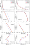 |
Fig. A.1 Cloud particle properties of the step-wise iterated cloud structure for the warm Saturn example HATS-6b. Iteration 5 is shown as a solid line to highlight the final result. Left: sub-stellar point. Right: anti-stellar point. Top: cloud mass fraction ρd/ρ. Upper middle: cloud particle number density nd. Lower middle: average cloud particle size ⟨a⟩. Bottom: Nucleation rate J⋆. The morning and evening terminator can be found in Fig 5. |
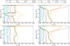 |
Fig. A.2 Cloud particle material composition of iteration 5. 1st row: Sub-stellar point. 2nd row: Anti-stellar point. 3rd row: Evening terminator. 4th row: Morning terminator. Here the cloud profiles only reach down to 0.3 bar. |
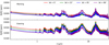 |
Fig. A.3 Transmission spectrum for each terminator grid cell. Top: Morning terminator. Bottom: Evening terminator. |
Appendix B Opacity data
The references for the absorption cross sections used in the radiative transfer of the GCM and transmission spectra calculations are listed in Table B.1. The references for the cloud particle material opacities are listed in Table B.2. Due to missing data, CaSiO3 is treated as vacuum.
References for cross sections of gas-phase species.
References for the cloud material opacities.
Appendix C GCM convergence tests
To test the convergence of the expeRT/MITgcm runs, we analyse the time dependent temperature evolution of the GCM. The results can be seen in Fig. C.1. The results show that the temperature structure of all three runs are reasonably converged in the upper layers of the GCM.
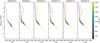 |
Fig. C.1 Evolution of the global average temperature for every 100 days of the expeRT/MITgcm runs. |
Appendix D Input SED for ARGO
The input SED used for the photo-chemistry of ARGO is shown in Fig. D.1. The SED is obtained from the MUSCLES survey where the star GJ667C is chosen as the closest analogue to HATS-6. The SED is combined from different spectra achieved through observations and models, as indicated in the sections separated by the dashed lines (see e.g. France et al. (2016) for details). The spectrum has been binned and adapted to the desired wavelength range 1-10,000 nm.
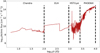 |
Fig. D.1 Input spectral energy distribution (SED) for host star expressed in actinic flux. |
References
- Ackerman, A. S., & Marley, M. S. 2001, ApJ, 556, 872 [Google Scholar]
- Adcroft, A., Campin, J.-M., Hill, C., & Marshall, J. 2004, Mon. Weather Rev., 132, 2845 [NASA ADS] [CrossRef] [Google Scholar]
- Agundez, M., Parmentier, V., Venot, O., Hersant, F., & Selsis, F. 2014, A&A, 564, A73 [NASA ADS] [CrossRef] [EDP Sciences] [Google Scholar]
- Ahrer, E.-M., Stevenson, K. B., Mansfield, M., et al. 2023, Nature, 614, 653 [NASA ADS] [CrossRef] [Google Scholar]
- Alderson, L., Wakeford, H. R., Alam, M. K., et al. 2023, Nature, 614, 664 [NASA ADS] [CrossRef] [Google Scholar]
- Alei, E., Konrad, B. S., Angerhausen, D., et al. 2022, A&A, 665, A106 [NASA ADS] [CrossRef] [EDP Sciences] [Google Scholar]
- Arfaux, A., & Lavvas, P. 2024, MNRAS, 530, 482 [NASA ADS] [CrossRef] [Google Scholar]
- Asplund, M., Grevesse, N., Sauval, A. J., & Scott, P. 2009, ARA&A, 47, 481 [NASA ADS] [CrossRef] [Google Scholar]
- Azzam, A. A. A., Tennyson, J., Yurchenko, S. N., & Naumenko, O. V. 2016, MNRAS, 460, 4063 [NASA ADS] [CrossRef] [Google Scholar]
- Baeyens, R. 2021, PhD thesis, On the Climate and Chemistry of Irradiated Exoplanet Atmospheres, KU Leuven [Google Scholar]
- Baeyens, R., Decin, L., Carone, L., et al. 2021, MNRAS, 505, 5603 [NASA ADS] [CrossRef] [Google Scholar]
- Baeyens, R., Konings, T., Venot, O., Carone, L., & Decin, L. 2022, MNRAS, 512, 4877 [NASA ADS] [CrossRef] [Google Scholar]
- Barber, R. J., Strange, J. K., Hill, C., et al. 2014, MNRAS, 437, 1828 [CrossRef] [Google Scholar]
- Barth, P., Helling, C., Stüeken, E. E., et al. 2021, MNRAS, 502, 6201 [Google Scholar]
- Batalha, N. E., Mandell, A., Pontoppidan, K., et al. 2017, PASP, 129, 064501 [Google Scholar]
- Bean, J. L., Miller-Ricci Kempton, E., & Homeier, D. 2010, Nature, 468, 669 [NASA ADS] [CrossRef] [Google Scholar]
- Begemann, B., Dorschner, J., Henning, T., et al. 1997, ApJ, 476, 199 [NASA ADS] [CrossRef] [Google Scholar]
- Benneke, B., Knutson, H. A., Lothringer, J., et al. 2019, Nat. Astron., 3, 813 [Google Scholar]
- Birkmann, S. M., Ferruit, P., Giardino, G., et al. 2022, A&A, 661, A83 [NASA ADS] [CrossRef] [EDP Sciences] [Google Scholar]
- Borysow, A. 2002, A&A, 390, 779 [NASA ADS] [CrossRef] [EDP Sciences] [Google Scholar]
- Borysow, A., & Frommhold, L. 1989, ApJ, 341, 549 [NASA ADS] [CrossRef] [Google Scholar]
- Borysow, J., Frommhold, L., & Birnbaum, G. 1988, ApJ, 326, 509 [NASA ADS] [CrossRef] [Google Scholar]
- Borysow, A., Frommhold, L., & Moraldi, M. 1989, ApJ, 336, 495 [NASA ADS] [CrossRef] [Google Scholar]
- Borysow, A., Jorgensen, U. G., & Fu, Y. 2001, JQSRT, 68, 235 [NASA ADS] [CrossRef] [Google Scholar]
- Bromley, S. T., Martín, J. C. G., & C. Plane, J. M. 2016, PCCP, 18, 26913 [NASA ADS] [CrossRef] [Google Scholar]
- Bruggeman, D. a. G. 1935, Ann. Phys., 416, 636 [CrossRef] [Google Scholar]
- Buchhave, L. A., Bitsch, B., Johansen, A., et al. 2018, ApJ, 856, 37 [Google Scholar]
- Carone, L., Baeyens, R., Mollière, P., et al. 2020, MNRAS, 496, 3582 [NASA ADS] [CrossRef] [Google Scholar]
- Carone, L., Mollière, P., Zhou, Y., et al. 2021, A&A, 646, A168 [NASA ADS] [CrossRef] [EDP Sciences] [Google Scholar]
- Carone, L., Lewis, D. A., Samra, D., Schneider, A. D., & Helling, C. 2023, arXiv e-prints [arXiv:2301.08492] [Google Scholar]
- Cañas, C. I., Kanodia, S., Bender, C. F., et al. 2022, AJ, 164, 50 [CrossRef] [Google Scholar]
- Chan, Y. M., & Dalgarno, A. 1965, Proc. Phys. Soc., 85, 227 [NASA ADS] [CrossRef] [Google Scholar]
- Charnay, B., Meadows, V., & Leconte, J. 2015a, ApJ, 813, 15 [Google Scholar]
- Charnay, B., Meadows, V., Misra, A., Leconte, J., & Arney, G. 2015b, ApJ, 813, L1 [NASA ADS] [CrossRef] [Google Scholar]
- Charnay, B., Bézard, B., Baudino, J. L., et al. 2018, ApJ, 854, 172 [Google Scholar]
- Christie, D. A., Mayne, N. J., Lines, S., et al. 2021, MNRAS, 506, 4500 [CrossRef] [Google Scholar]
- Christie, D. A., Mayne, N. J., Gillard, R. M., et al. 2022, MNRAS, 517, 1407 [NASA ADS] [CrossRef] [Google Scholar]
- Coles, P. A., Yurchenko, S. N., & Tennyson, J. 2019, MNRAS, 490, 4638 [CrossRef] [Google Scholar]
- Cowan, N. B., Machalek, P., Croll, B., et al. 2012, ApJ, 747, 82 [Google Scholar]
- Crossfield, I. J. M. 2015, PASP, 127, 941 [NASA ADS] [CrossRef] [Google Scholar]
- Crossfield, I. J. M., Barman, T., Hansen, B. M. S., & Howard, A. W. 2013, A&A, 559, A33 [NASA ADS] [CrossRef] [EDP Sciences] [Google Scholar]
- Dalgarno, A., & Williams, D. A. 1962, ApJ, 136, 690 [NASA ADS] [CrossRef] [Google Scholar]
- Dang, L., Cowan, N. B., Schwartz, J. C., et al. 2018, Nat. Astron., 2, 220 [NASA ADS] [CrossRef] [Google Scholar]
- Dominik, C., Sedlmayr, E., & Gail, H.-P. 1993, A&A, 277, 578 [NASA ADS] [Google Scholar]
- Demory, B.-O., Wit, J. d., Lewis, N., et al. 2013, ApJ, 776, L25 [CrossRef] [Google Scholar]
- Dorschner, J., Begemann, B., Henning, T., Jaeger, C., & Mutschke, H. 1995, A&A, 300, 503 [Google Scholar]
- Dyrek, A., Min, M., Decin, L., et al. 2023, Nature, 625, 51 [Google Scholar]
- Espinoza, N., Steinrueck, M. E., Kirk, J., et al. 2024, Nature, 632, 1017 [CrossRef] [Google Scholar]
- Estrela, R., Swain, M. R., & Roudier, G. M. 2022, ApJ, 941, L5 [NASA ADS] [CrossRef] [Google Scholar]
- Feautrier, P. 1964, Comp. Rend. Acad. Sci. Paris, 258, 3189 [NASA ADS] [Google Scholar]
- Feinstein, A. D., Radica, M., Welbanks, L., et al. 2023, Nature, 614, 670 [NASA ADS] [CrossRef] [Google Scholar]
- Ferruit, P., Jakobsen, P., Giardino, G., et al. 2022, A&A, 661, A81 [NASA ADS] [CrossRef] [EDP Sciences] [Google Scholar]
- Fischer, P. D., Knutson, H. A., Sing, D. K., et al. 2016, ApJ, 827, 19 [CrossRef] [Google Scholar]
- Fortney, J. J., Lodders, K., Marley, M. S., & Freedman, R. S. 2008, ApJ, 678, 1419 [CrossRef] [Google Scholar]
- Fortney, J. J., Visscher, C., Marley, M. S., et al. 2020, AJ, 160, 288 [NASA ADS] [CrossRef] [Google Scholar]
- France, K., Loyd, R. O. P., Youngblood, A., et al. 2016, ApJ, 820, 89 [NASA ADS] [CrossRef] [Google Scholar]
- Fraschetti, F., Drake, J. J., Alvarado-Gómez, J. D., et al. 2019, ApJ, 874, 21 [NASA ADS] [CrossRef] [Google Scholar]
- Gail, H.-P., & Sedlmayr, E. 1986, A&A, 166, 225 [NASA ADS] [Google Scholar]
- Gail, H.-P., & Sedlmayr, E. 1988, A&A, 206, 153 [NASA ADS] [Google Scholar]
- Gandhi, S., & Madhusudhan, N. 2019, MNRAS, 485, 5817 [Google Scholar]
- Gao, P., & Benneke, B. 2018, ApJ, 863, 165 [CrossRef] [Google Scholar]
- Gao, P., Thorngren, D. P., Lee, E. K. H., et al. 2020, Nat. Astron., 4, 951 [NASA ADS] [CrossRef] [Google Scholar]
- Gobrecht, D., Plane, J. M. C., Bromley, S. T., et al. 2022, A&A, 658, A167 [NASA ADS] [CrossRef] [EDP Sciences] [Google Scholar]
- Gobrecht, D., Hashemi, S. R., Plane, J. M. C., et al. 2023, A&A, 680, A18 [NASA ADS] [CrossRef] [EDP Sciences] [Google Scholar]
- Grant, D., Lewis, N. K., Wakeford, H. R., et al. 2023, ApJ, 956, L29 [Google Scholar]
- Gray, D. F. 2008, The Observation and Analysis of Stellar Photospheres (Cambridge University Press) [Google Scholar]
- Harada, C. K., Kempton, E. M.-R., Rauscher, E., et al. 2021, ApJ, 909, 85 [NASA ADS] [CrossRef] [Google Scholar]
- Harris, C. R., Millman, K. J., van der Walt, S. J., et al. 2020, Nature, 585, 357 [NASA ADS] [CrossRef] [Google Scholar]
- Hartman, J. D., Bayliss, D., Brahm, R., et al. 2015, ApJ, 149, 166 [CrossRef] [Google Scholar]
- Haynes, K., Mandell, A. M., Madhusudhan, N., Deming, D., & Knutson, H. 2015, ApJ, 806, 146 [NASA ADS] [CrossRef] [Google Scholar]
- Helling, C., & Woitke, P. 2006, A&A, 455, 325 [NASA ADS] [CrossRef] [EDP Sciences] [Google Scholar]
- Helling, C., & Fomins, A. 2013, Phil. Trans. R. Soc. A, 371, 20110581 [CrossRef] [Google Scholar]
- Helling, C., Oevermann, M., Lüttke, M. J. H., Klein, R., & Sedlmayr, E. 2001, A&A, 376, 194 [NASA ADS] [CrossRef] [EDP Sciences] [Google Scholar]
- Helling, C., Klein, R., Woitke, P., Nowak, U., & Sedlmayr, E. 2004, A&A, 423, 657 [NASA ADS] [CrossRef] [EDP Sciences] [Google Scholar]
- Helling, C., Dehn, M., Woitke, P., & Hauschildt, P. H. 2008a, ApJ, 675, L105 [NASA ADS] [CrossRef] [Google Scholar]
- Helling, C., Woitke, P., & Thi, W.-F. 2008b, A&A, 485, 547 [NASA ADS] [CrossRef] [EDP Sciences] [Google Scholar]
- Helling, C., Lee, E., Dobbs-Dixon, I., et al. 2016, MNRAS, 460, 855 [NASA ADS] [CrossRef] [Google Scholar]
- Helling, C., Tootill, D., Woitke, P., & Lee, E. K. H. 2017, A&A, 603, A123 [NASA ADS] [CrossRef] [EDP Sciences] [Google Scholar]
- Helling, C., Gourbin, P., Woitke, P., & Parmentier, V. 2019a, A&A, 626, A133 [NASA ADS] [CrossRef] [EDP Sciences] [Google Scholar]
- Helling, C., Iro, N., Corrales, L., et al. 2019b, A&A, 631, A79 [NASA ADS] [CrossRef] [EDP Sciences] [Google Scholar]
- Helling, C., Kawashima, Y., Graham, V., et al. 2020, A&A, 641, A178 [NASA ADS] [CrossRef] [EDP Sciences] [Google Scholar]
- Helling, C., Lewis, D., Samra, D., et al. 2021, A&A, 649, A44 [NASA ADS] [CrossRef] [EDP Sciences] [Google Scholar]
- Helling, C., Samra, D., Lewis, D., et al. 2023, A&A, 671, A122 [NASA ADS] [CrossRef] [EDP Sciences] [Google Scholar]
- Heng, K., Hayek, W., Pont, F., & Sing, D. K. 2012, MNRAS, 420, 20 [NASA ADS] [CrossRef] [Google Scholar]
- Henning, T., Begemann, B., Mutschke, H., & Dorschner, J. 1995, A&ASS, 112, 143 [NASA ADS] [Google Scholar]
- Hobbs, R., Rimmer, P. B., Shorttle, O., & Madhusudhan, N. 2021, MNRAS, 506, 3186 [NASA ADS] [CrossRef] [Google Scholar]
- Holton, J. R., & Hakim, G. J. 2013, An Introduction to Dynamic Meteorology, 5th edn. (Amsterdam: Academic Press) [Google Scholar]
- Hu, Y., & Ding, F. 2011, A&A, 526, A135 [NASA ADS] [CrossRef] [EDP Sciences] [Google Scholar]
- Hubeny, I., Burrows, A., & Sudarsky, D. 2003, ApJ, 594, 1011 [Google Scholar]
- Hunter, J. D. 2007, Comput. Sci. Eng., 9, 90 [NASA ADS] [CrossRef] [Google Scholar]
- Hünsch, M., Weidner, C., & Schmitt, J. H. M. M. 2003, A&A, 402, 571 [NASA ADS] [CrossRef] [EDP Sciences] [Google Scholar]
- Juncher, D., Jørgensen, U. G., & Helling, C. 2017, A&A, 608, A70 [NASA ADS] [CrossRef] [EDP Sciences] [Google Scholar]
- JWST Transiting Exoplanet Community Early Release Science-Team, Ahrer, E.-M., Alderson, L., et al. 2023, Nature, 614, 649 [NASA ADS] [CrossRef] [Google Scholar]
- Kataria, T., Sing, D. K., Lewis, N. K., et al. 2016, ApJ, 821, 9 [NASA ADS] [CrossRef] [Google Scholar]
- Kempton, E. M.-R., Bean, J. L., & Parmentier, V. 2017, ApJ, 845, L20 [NASA ADS] [CrossRef] [Google Scholar]
- Kendrew, S., Scheithauer, S., Bouchet, P., et al. 2015, PASP, 127, 623 [NASA ADS] [CrossRef] [Google Scholar]
- Kendrew, S., Scheithauer, S., Bouchet, P., et al. 2016, Proc. SPIE, 9904, 990443 [NASA ADS] [CrossRef] [Google Scholar]
- Kiefer, S., Gobrecht, D., Decin, L., & Helling, C. 2023, A&A, 671, A169 [NASA ADS] [CrossRef] [EDP Sciences] [Google Scholar]
- Kiefer, S., Lecoq-Molinos, H., Helling, C., Bangera, N., & Decin, L. 2024, A&A, 682, A150 [NASA ADS] [CrossRef] [EDP Sciences] [Google Scholar]
- Knutson, H. A., Charbonneau, D., Allen, L. E., et al. 2007, Nature, 447, 183 [NASA ADS] [CrossRef] [Google Scholar]
- Knutson, H. A., Dragomir, D., Kreidberg, L., et al. 2014, ApJ, 794, 155 [Google Scholar]
- Komacek, T. D., & Showman, A. P. 2016, ApJ, 821, 16 [CrossRef] [Google Scholar]
- Komacek, T. D., Showman, A. P., & Tan, X. 2017, ApJ, 835, 198 [NASA ADS] [CrossRef] [Google Scholar]
- Komacek, T. D., Showman, A. P., & Parmentier, V. 2019, ApJ, 881, 152 [Google Scholar]
- Komacek, T. D., Fauchez, T. J., Wolf, E. T., & Abbot, D. S. 2020, ApJ, 888, L20 [Google Scholar]
- Komacek, T. D., Tan, X., Gao, P., & Lee, E. K. H. 2022, ApJ, 934, 79 [NASA ADS] [CrossRef] [Google Scholar]
- Konings, T., Baeyens, R., & Decin, L. 2022, A&A, 667, A15 [NASA ADS] [CrossRef] [EDP Sciences] [Google Scholar]
- Kreidberg, L., Bean, J. L., Désert, J.-M., et al. 2014, Nature, 505, 69 [Google Scholar]
- Köhn, C., Helling, C., Enghoff, M. B., et al. 2021, A&A, 654, A120 [NASA ADS] [CrossRef] [EDP Sciences] [Google Scholar]
- Lacy, B. I., & Burrows, A. 2020, ApJ, 905, 131 [NASA ADS] [CrossRef] [Google Scholar]
- Lecoq-Molinos, H., Gobrecht, D., Sindel, J. P., Helling, C., & Decin, L. 2024, A&A, 690, A34 [NASA ADS] [CrossRef] [EDP Sciences] [Google Scholar]
- Lee, E. K. H. 2023, MNRAS, 524, 2918 [NASA ADS] [CrossRef] [Google Scholar]
- Lee, E. K. H., Blecic, J., & Helling, C. 2018, A&A, 614, A126 [NASA ADS] [CrossRef] [EDP Sciences] [Google Scholar]
- Lee, E. K. H., Helling, C., Giles, H., & Bromley, S. T. 2015, A&A, 575, A11 [NASA ADS] [CrossRef] [EDP Sciences] [Google Scholar]
- Lee, E. K. H., Dobbs-Dixon, I., Helling, C., Bognar, K., & Woitke, P. 2016, A&A, 594, A48 [NASA ADS] [CrossRef] [EDP Sciences] [Google Scholar]
- Lee, E. K. H., Wood, K., Dobbs-Dixon, I., Rice, A., & Helling, C. 2017, A&A, 601, A22 [NASA ADS] [CrossRef] [EDP Sciences] [Google Scholar]
- Lee, E., Taylor, J., Grimm, S. L., et al. 2019, MNRAS, 487, 2082 [NASA ADS] [CrossRef] [Google Scholar]
- Lee, E. K. H., Parmentier, V., Hammond, M., et al. 2021, MNRAS, 506, 2695 [NASA ADS] [CrossRef] [Google Scholar]
- Lee, E. K. H., Tsai, S.-M., Hammond, M., & Tan, X. 2023, A&A, 672, A110 [NASA ADS] [CrossRef] [EDP Sciences] [Google Scholar]
- Li, G., Gordon, I. E., Rothman, L. S., et al. 2015, ApJSS, 216, 15 [NASA ADS] [CrossRef] [Google Scholar]
- Lin, A. S. J., Libby-Roberts, J. E., Alvarado-Montes, J. A., et al. 2023, AJ, 166, 90 [NASA ADS] [CrossRef] [Google Scholar]
- Line, M. R., & Parmentier, V. 2016, ApJ, 820, 78 [Google Scholar]
- Line, M. R., Vasisht, G., Chen, P., Angerhausen, D., & Yung, Y. L. 2011, ApJ, 738, 32 [NASA ADS] [CrossRef] [Google Scholar]
- Lines, S., Manners, J., Mayne, N. J., et al. 2018a, MNRAS, 481, 194 [NASA ADS] [CrossRef] [Google Scholar]
- Lines, S., Mayne, N. J., Boutle, I. A., et al. 2018b, A&A, 615, A97 [NASA ADS] [CrossRef] [EDP Sciences] [Google Scholar]
- Looyenga, H. 1965, Physica, 31, 401 [NASA ADS] [CrossRef] [Google Scholar]
- Lothringer, J. D., & Barman, T. 2019, ApJ, 876, 69 [Google Scholar]
- Loyd, R. O. P., France, K., Youngblood, A., et al. 2016, ApJ, 824, 102 [NASA ADS] [CrossRef] [Google Scholar]
- Loyd, R. O. P., France, K., Youngblood, A., et al. 2018, ApJ, 867, 71 [Google Scholar]
- McKay, C. P., Pollack, J. B., & Courtin, R. 1991, Science, 253, 1118 [NASA ADS] [CrossRef] [Google Scholar]
- McKemmish, L. K., Yurchenko, S. N., & Tennyson, J. 2016, MNRAS, 463, 771 [NASA ADS] [CrossRef] [Google Scholar]
- McKemmish, L. K., Masseron, T., Hoeijmakers, H. J., et al. 2019, MNRAS, 488, 2836 [Google Scholar]
- Mie, G. 1908, Ann. Phys., 330, 377 [Google Scholar]
- Mignon, L., Meunier, N., Delfosse, X., et al. 2023, A&A, 675, A168 [NASA ADS] [CrossRef] [EDP Sciences] [Google Scholar]
- Min, M., Ormel, C. W., Chubb, K., Helling, C., & Kawashima, Y. 2020, A&A, 642, A28 [NASA ADS] [CrossRef] [EDP Sciences] [Google Scholar]
- Mollière, P., Wardenier, J. P., Boekel, R. v., et al. 2019, A&A, 627, A67 [NASA ADS] [CrossRef] [EDP Sciences] [Google Scholar]
- Mollière, P., Stolker, T., Lacour, S., et al. 2020, A&A, 640, A131 [Google Scholar]
- Morley, C. V., Fortney, J. J., Marley, M. S., et al. 2012, ApJ, 756, 172 [NASA ADS] [CrossRef] [Google Scholar]
- Moses, J. I., Visscher, C., Fortney, J. J., et al. 2011, ApJ, 737, 15 [Google Scholar]
- Mukherjee, S., Batalha, N. E., & Marley, M. S. 2021, ApJ, 910, 158 [NASA ADS] [CrossRef] [Google Scholar]
- Namekata, K., Maehara, H., Sasaki, R., et al. 2020, PASJ, 72, 68 [NASA ADS] [CrossRef] [Google Scholar]
- Nikolov, N., Sing, D. K., Gibson, N. P., et al. 2016, ApJ, 832, 191 [NASA ADS] [CrossRef] [Google Scholar]
- Nixon, M. C., & Madhusudhan, N. 2022, ApJ, 935, 73 [NASA ADS] [CrossRef] [Google Scholar]
- Olson, G. L., Auer, L. H., & Buchler, J. R. 1986, JQSRT, 35, 431 [NASA ADS] [CrossRef] [Google Scholar]
- Ormel, C. W., & Min, M. 2019, A&A, 622, A121 [NASA ADS] [CrossRef] [EDP Sciences] [Google Scholar]
- Palik, E. D. 1985, ed. E. D. Palik, Academic Press Handbook Series (New York: Academic Press) [Google Scholar]
- Parmentier, V., Fortney, J. J., Showman, A. P., Morley, C., & Marley, M. S. 2016, ApJ, 828, 22 [Google Scholar]
- Parmentier, V., Showman, A. P., & Lian, Y. 2013, A&A, 558, A91 [NASA ADS] [CrossRef] [EDP Sciences] [Google Scholar]
- Parmentier, V., Line, M. R., Bean, J. L., et al. 2018, A&A, 617, A110 [NASA ADS] [CrossRef] [EDP Sciences] [Google Scholar]
- Parmentier, V., Showman, A. P., & Fortney, J. J. 2021, MNRAS, 501, 78 [Google Scholar]
- Pascucci, I., Testi, L., Herczeg, G. J., et al. 2016, ApJ, 831, 125 [Google Scholar]
- Pelletier, S., Benneke, B., Ali-Dib, M., et al. 2023, Nature, 619, 491 [NASA ADS] [CrossRef] [Google Scholar]
- Perez-Becker, D., & Showman, A. P. 2013, ApJ, 776, 134 [NASA ADS] [CrossRef] [Google Scholar]
- Piskunov, N. E., Kupka, F., Ryabchikova, T. A., Weiss, W. W., & Jeffery, C. S. 1995, A&ASS, 112, 525 [NASA ADS] [Google Scholar]
- Polyansky, O. L., Kyuberis, A. A., Zobov, N. F., et al. 2018, MNRAS, 480, 2597 [NASA ADS] [CrossRef] [Google Scholar]
- Posch, T., Kerschbaum, F., Fabian, D., et al. 2003, ApJS, 149, 437 [NASA ADS] [CrossRef] [Google Scholar]
- Powell, D., & Zhang, X. 2024, arXiv e-prints [arXiv:2404.08759] [Google Scholar]
- Powell, D., Louden, T., Kreidberg, L., et al. 2019, ApJ, 887, 170 [NASA ADS] [CrossRef] [Google Scholar]
- Powell, D., Zhang, X., Gao, P., & Parmentier, V. 2018, ApJ, 860, 18 [Google Scholar]
- Querry, M. R. 1998, Optical Constants of Minerals and Other Materials from the Millimeter to the Ultraviolet (Chemical Research, Development & Engineering Center, U.S. Army Armament Munitions Chemical Command) [Google Scholar]
- Richard, C., Gordon, I. E., Rothman, L. S., et al. 2012, JQSRT, 113, 1276 [NASA ADS] [CrossRef] [Google Scholar]
- Rimmer, P. B., & Helling, C. 2013, ApJ, 774, 108 [NASA ADS] [CrossRef] [Google Scholar]
- Rimmer, P. B., & Helling, C. 2016, ApJS, 224, 9 [NASA ADS] [CrossRef] [Google Scholar]
- Rimmer, P. B., & Helling, C. 2019, ApJS, 245, 20 [NASA ADS] [CrossRef] [Google Scholar]
- Rimmer, P. B., & Rugheimer, S. 2019, Icarus, 329, 124 [CrossRef] [Google Scholar]
- Robbins-Blanch, N., Kataria, T., Batalha, N. E., & Adams, D. J. 2022, ApJ, 930, 93 [NASA ADS] [CrossRef] [Google Scholar]
- Rodgers-Lee, D., Rimmer, P. B., Vidotto, A. A., et al. 2023, MNRAS, 521, 5880 [NASA ADS] [CrossRef] [Google Scholar]
- Roman, M., & Rauscher, E. 2017, ApJ, 850, 17 [NASA ADS] [CrossRef] [Google Scholar]
- Roman, M., & Rauscher, E. 2019, ApJ, 872, 1 [NASA ADS] [CrossRef] [Google Scholar]
- Roman, M. T., Kempton, E. M.-R., Rauscher, E., et al. 2021, ApJ, 908, 101 [CrossRef] [Google Scholar]
- Rowe, J. F., Matthews, J. M., Seager, S., et al. 2008, ApJ, 689, 1345 [Google Scholar]
- Rustamkulov, Z., Sing, D. K., Mukherjee, S., et al. 2023, Nature, 614, 659 [NASA ADS] [CrossRef] [Google Scholar]
- Samra, D., Helling, C., & Min, M. 2020, A&A, 639, A107 [NASA ADS] [CrossRef] [EDP Sciences] [Google Scholar]
- Samra, D., Helling, C., Chubb, K. L., et al. 2023, A&A, 669, A142 [NASA ADS] [CrossRef] [EDP Sciences] [Google Scholar]
- Savel, A. B., Kempton, E. M.-R., Malik, M., et al. 2022, ApJ, 926, 85 [NASA ADS] [CrossRef] [Google Scholar]
- Schneider, A. D., Baeyens, R., & Kiefer, S. 2022a, https://doi.org/10.5281/zenodo.7116787 [Google Scholar]
- Schneider, A. D., Carone, L., Decin, L., Jørgensen, U. G., & Helling, C. 2022b, A&A, 666, L11 [NASA ADS] [CrossRef] [EDP Sciences] [Google Scholar]
- Schneider, A. D., Carone, L., Decin, L., et al. 2022c, A&A, 664, A56 [NASA ADS] [CrossRef] [EDP Sciences] [Google Scholar]
- Showman, A. P., & Guillot, T. 2002, A&A, 385, 166 [NASA ADS] [CrossRef] [EDP Sciences] [Google Scholar]
- Showman, A. P., & Polvani, L. M. 2011, ApJ, 738, 71 [Google Scholar]
- Showman, A. P., Fortney, J. J., Lian, Y., et al. 2009, ApJ, 699, 564 [NASA ADS] [CrossRef] [Google Scholar]
- Sindel, J. P., Gobrecht, D., Helling, C., & Decin, L. 2022, A&A, 668, A35 [NASA ADS] [CrossRef] [EDP Sciences] [Google Scholar]
- Sing, D. K., Wakeford, H. R., Showman, A. P., et al. 2015, MNRAS, 446, 2428 [NASA ADS] [CrossRef] [Google Scholar]
- Sing, D. K., Fortney, J. J., Nikolov, N., et al. 2016, Nature, 529, 59 [Google Scholar]
- Skinner, J. W., & Cho, J. Y.-K. 2022, MNRAS, 511, 3584 [NASA ADS] [CrossRef] [Google Scholar]
- Sousa-Silva, C., Al-Refaie, A. F., Tennyson, J., & Yurchenko, S. N. 2015 MNRAS, 446, 2337 [Google Scholar]
- Steinrueck, M. E., Parmentier, V., Showman, A. P., Lothringer, J. D., & Lupu, R. E. 2019, ApJ, 880, 14 [Google Scholar]
- Steinrueck, M. E., Showman, A. P., Lavvas, P., et al. 2021, MNRAS, 504, 2783 [NASA ADS] [CrossRef] [Google Scholar]
- Steinrueck, M. E., Koskinen, T., Lavvas, P., et al. 2023, ApJ, 951, 117 [NASA ADS] [CrossRef] [Google Scholar]
- Suto, H., Sogawa, H., Tachibana, S., et al. 2006, MNRAS, 370, 1599 [CrossRef] [Google Scholar]
- Tan, X., & Showman, A. P. 2017, ApJ, 835, 186 [NASA ADS] [CrossRef] [Google Scholar]
- Tan, X., & Showman, A. P. 2021, MNRAS, 502, 2198 [NASA ADS] [CrossRef] [Google Scholar]
- Thorngren, D., Gao, P., & Fortney, J. J. 2019, ApJ, 884, L6 [Google Scholar]
- Tsai, S.-M., Lyons, J. R., Grosheintz, L., et al. 2017, ApJS, 228, 20 [NASA ADS] [CrossRef] [Google Scholar]
- Tsai, S.-M., Lee, E. K. H., Powell, D., et al. 2023, Nature, 617, 483 [CrossRef] [Google Scholar]
- Turbet, M., Bolmont, E., Chaverot, G., et al. 2021, Nature, 598, 276 [CrossRef] [Google Scholar]
- Venot, O., Rocchetto, M., Carl, S., Roshni Hashim, A., & Decin, L. 2016, ApJ, 830, 77 [NASA ADS] [CrossRef] [Google Scholar]
- Vuitton, V. 2021, in Encyclopedia of Geology (Elsevier), 217 [Google Scholar]
- Wakeford, H. R., & Sing, D. K. 2015, A&A, 573, A122 [NASA ADS] [CrossRef] [EDP Sciences] [Google Scholar]
- Wakeford, H. R., Sing, D. K., Deming, D., et al. 2018, ApJ, 155, 29 [CrossRef] [Google Scholar]
- Wang, H., & Wordsworth, R. 2020, ApJ, 891, 7 [NASA ADS] [CrossRef] [Google Scholar]
- Webber, M. W., Lewis, N. K., Marley, M., et al. 2015, ApJ, 804, 94 [NASA ADS] [CrossRef] [Google Scholar]
- Wende, S., Reiners, A., Seifahrt, A., & Bernath, P. F. 2010, A&A, 523, A58 [NASA ADS] [CrossRef] [EDP Sciences] [Google Scholar]
- Witte, S., Helling, C., Barman, T., Heidrich, N., & Hauschildt, P. H. 2011, A&A, 529, A44 [NASA ADS] [CrossRef] [EDP Sciences] [Google Scholar]
- Woitke, P., & Helling, C. 2003, A&A, 399, 297 [NASA ADS] [CrossRef] [EDP Sciences] [Google Scholar]
- Woitke, P., & Helling, C. 2004, A&A, 414, 335 [NASA ADS] [CrossRef] [EDP Sciences] [Google Scholar]
- Woitke, P., Helling, C., Hunter, G. H., et al. 2018, A&A, 614, A1 [NASA ADS] [CrossRef] [EDP Sciences] [Google Scholar]
- Woitke, P., Helling, C., & Gunn, O. 2020, A&A, 634, A23 [NASA ADS] [CrossRef] [EDP Sciences] [Google Scholar]
- Wong, I., Chachan, Y., Knutson, H. A., et al. 2022, AJ, 164, 30 [NASA ADS] [CrossRef] [Google Scholar]
- Yang, J., Boué, G., Fabrycky, D. C., & Abbot, D. S. 2014, ApJ, 787, L2 [NASA ADS] [CrossRef] [Google Scholar]
- Yan, F., Pallé, E., Reiners, A., et al. 2020, A&A, 640, L5 [NASA ADS] [CrossRef] [EDP Sciences] [Google Scholar]
- Yan, F., Reiners, A., Pallé, E., et al. 2022, A&A, 659, A7 [NASA ADS] [CrossRef] [EDP Sciences] [Google Scholar]
- Youngblood, A., France, K., Loyd, R. O. P., et al. 2016, ApJ, 824, 101 [Google Scholar]
- Youngblood, A., France, K., Loyd, R. O. P., et al. 2017, ApJ, 843, 31 [Google Scholar]
- Yurchenko, S. N., Amundsen, D. S., Tennyson, J., & Waldmann, I. P. 2017, A&A, 605, A95 [NASA ADS] [CrossRef] [EDP Sciences] [Google Scholar]
- Yurchenko, S. N., Mellor, T. M., Freedman, R. S., & Tennyson, J. 2020, MNRAS, 496, 5282 [NASA ADS] [CrossRef] [Google Scholar]
- Zamyatina, M., Christie, D. A., Hébrard, E., et al. 2024, MNRAS, 529, 1776 [NASA ADS] [CrossRef] [Google Scholar]
- Zeidler, S., Posch, T., Mutschke, H., Richter, H., & Wehrhan, O. 2011, A&A, 526, A68 [NASA ADS] [CrossRef] [EDP Sciences] [Google Scholar]
- Zeidler, S., Posch, T., & Mutschke, H. 2013, A&A, 553, A81 [NASA ADS] [CrossRef] [EDP Sciences] [Google Scholar]
C32 corresponds to a resolution of 128x64 in longitude and latitude.
This is a typical choice for hot Jupiters (see, e.g. Showman et al. 2009; Lee et al. 2021; Schneider et al. 2022c,b)
References can be found in Table B.1.
References can be found in Table B.1.
Also sometimes called dust-to-gas ratio.
This resolution was chosen to maximise the spectral precision while keeping enough data points to detect gas-phase features.
Convergence is here defined as ∇ · v < 0, where v is the horizontal velocity vector.
All Tables
All Figures
|
Fig. 1 Known gas giants and JWST targets. The blue shaded area represents the approximate parameter space of warm Saturns. Several often studied exoplanets are shown. |
| In the text | |
|
Fig. 2 (Tgas, pgas) profiles of the sub-stellar point, anti-stellar point, evening terminator, and morning terminator. |
| In the text | |
|
Fig. 3 Isobaric slices of the expeRT/MITgcm runs at t = 2000 simulation days. The white lines indicate the horizontal wind velocity fields. |
| In the text | |
|
Fig. 4 Zonally averaged zonal wind velocities at t = 2000 simulation days. |
| In the text | |
|
Fig. 5 Cloud particle properties of the step-wise iterated cloud structure for the warm Saturn example HATS-6b. Iteration 5 is shown as a solid line to highlight the final result. Left: morning terminator. Right: evening terminator. Top: cloud mass fraction ρd/ρ. Upper middle: cloud particle number density nd. Lower middle: average cloud particle size ⟨a⟩. Bottom: nucleation rate J⋆. The sub- and anti-stellar point are shown in Fig. A.1. |
| In the text | |
|
Fig. 6 Concentrations of non-equilibrium gas species for the warm Saturn example HATS-6b. Top: terminator region (both morning and evening) averaged over all six coordinates for all iterations. Middle: sub- and anti-stellar point for the final iteration (Iteration 5). Bottom: morning and evening terminators for the final iteration (Iteration 5). |
| In the text | |
|
Fig. 7 Comparison of the transmission spectra for the warm Saturn example HATS-6b for λ = 0.3 μm to 25 μm Top: transmission spectrum for each iteration. Bottom: absolute residuals between subsequent iterations and the spectral precision for JWST observations with NIRspec Prism and MIRI LRS for two and ten transits. |
| In the text | |
|
Fig. 8 Cloud structure of the morning (left) and evening (right) terminator of HATS-6b. Top: gas temperature Tgas and total J⋆ and JTiO2, and JSiO. Middle: gas-phase relative concentrations ni/ngas and cloud mass fraction ρd/ρ. Bottom: cloud particle volume fractions Vs/Vtot and mean cloud particle size ⟨a⟩. Salts are a minor component and have a volume fraction close to 0. |
| In the text | |
|
Fig. 9 Transmission spectra for the warm Saturn HATS-6b for λ = 0.3 μm to 25 μm including the total spectrum of the final iteration (iteration 5) and the morning and evening terminator separately. We also show the contributions of selected gas-phase species, the contribution of the Si-bearing cloud particle materials, and the spectral accuracy of the JWST instruments NIRSpec prism and MIRI LRS for two and ten transits. |
| In the text | |
|
Fig. 10 Potential temperature cross section across the morning (left panels) and evening terminators (right panels) for iterations 0 to 5 (from top to bottom). |
| In the text | |
|
Fig. A.1 Cloud particle properties of the step-wise iterated cloud structure for the warm Saturn example HATS-6b. Iteration 5 is shown as a solid line to highlight the final result. Left: sub-stellar point. Right: anti-stellar point. Top: cloud mass fraction ρd/ρ. Upper middle: cloud particle number density nd. Lower middle: average cloud particle size ⟨a⟩. Bottom: Nucleation rate J⋆. The morning and evening terminator can be found in Fig 5. |
| In the text | |
|
Fig. A.2 Cloud particle material composition of iteration 5. 1st row: Sub-stellar point. 2nd row: Anti-stellar point. 3rd row: Evening terminator. 4th row: Morning terminator. Here the cloud profiles only reach down to 0.3 bar. |
| In the text | |
|
Fig. A.3 Transmission spectrum for each terminator grid cell. Top: Morning terminator. Bottom: Evening terminator. |
| In the text | |
|
Fig. C.1 Evolution of the global average temperature for every 100 days of the expeRT/MITgcm runs. |
| In the text | |
|
Fig. D.1 Input spectral energy distribution (SED) for host star expressed in actinic flux. |
| In the text | |
Current usage metrics show cumulative count of Article Views (full-text article views including HTML views, PDF and ePub downloads, according to the available data) and Abstracts Views on Vision4Press platform.
Data correspond to usage on the plateform after 2015. The current usage metrics is available 48-96 hours after online publication and is updated daily on week days.
Initial download of the metrics may take a while.