| Issue |
A&A
Volume 698, June 2025
|
|
|---|---|---|
| Article Number | A39 | |
| Number of page(s) | 19 | |
| Section | Stellar structure and evolution | |
| DOI | https://doi.org/10.1051/0004-6361/202452949 | |
| Published online | 28 May 2025 | |
Binarity at LOw Metallicity (BLOeM)
The multiplicity properties and evolution of BAF-type supergiants⋆
1
Centro de Astrobiología (CSIC-INTA), Ctra. Torrejón a Ajalvir km 4, 28850 Torrejón de Ardoz, Spain
2
Instituto de Astrofísica de Canarias, C. Vía Láctea, s/n, 38205 La Laguna, Santa Cruz de Tenerife, Spain
3
The School of Physics and Astronomy, Tel Aviv University, Tel Aviv 6997801, Israel
4
ESO – European Southern Observatory, Karl-Schwarzschild-Strasse 2, 85748 Garching bei München, Germany
5
Institute of Astronomy, KU Leuven, Celestijnenlaan 200D, 3001 Leuven, Belgium
6
Department of Physics & Astronomy, Hounsfield Road, University of Sheffield, Sheffield S3 7RH, United Kingdom
7
Royal Observatory of Belgium, Avenue Circulaire/Ringlaan 3, B-1180 Brussels, Belgium
8
Argelander-Institut für Astronomie, Universität Bonn, Auf dem Hügel 71, 53121 Bonn, Germany
9
European Space Agency (ESA), ESA Office, Space Telescope Science Institute, 3700 San Martin Drive, Baltimore, MD 21218, USA
10
Institute of Science and Technology Austria (ISTA), Am Campus 1, 3400 Klosterneuburg, Austria
11
Max-Planck-Institute for Astrophysics, Karl-Schwarzschild-Strasse 1, 85748 Garching, Germany
12
Zentrum für Astronomie der Universität Heidelberg, Astronomisches Rechen-Institut, Mönchhofstr. 12-14, 69120 Heidelberg, Germany
13
School of Mathematics, Statistics and Physics, Newcastle University, Newcastle upon Tyne NE1 7RU, UK
14
Heidelberger Institut für Theoretische Studien, Schloss-Wolfsbrunnenweg 35, 69118 Heidelberg, Germany
15
McWilliams Center for Cosmology & Astrophysics, Department of Physics, Carnegie Mellon University, Pittsburgh, PA 15213, USA
16
Max-Planck-Institut für Astronomie, Königstuhl 17, D-69117 Heidelberg, Germany
17
Anton Pannekoek Institute for Astronomy, University of Amsterdam, Science Park 904, 1098 XH Amsterdam, The Netherlands
18
Institute of Astronomy, University of Cambridge, Madingley Road, Cambridge CB3 0HA, United Kingdom
19
Gemini Observatory/NSF’s NOIRLab, Casilla 603, La Serena, Chile
20
Center for Computational Astrophysics, Division of Science, National Astronomical Observatory of Japan, 2-21-1, Osawa, Mitaka, Tokyo 181-8588, Japan
21
School of Physics and Astronomy, Monash University, Clayton, VIC 3800, Australia
22
ARC Centre of Excellence for Gravitational-wave Discovery (OzGrav), Melbourne, Australia
23
Department of Astronomy, Pupin Hall, Columbia University, New York City, NY 10027, USA
24
Department of Physics and Astronomy, University of Wyoming, 1000 E. University Ave., Dept. 3905, Laramie, WY 82071, USA
25
Institut für Physik und Astronomie, Universität Potsdam, Karl-Liebknecht-Str. 24/25, 14476 Potsdam, Germany
26
Department of Astronomy & Steward Observatory, 933 N. Cherry Ave., Tucson, AZ 85721, USA
27
Institute of Astronomy, Faculty of Physics, Astronomy and Informatics, Nicolaus Copernicus University, Grudziadzka 5, 87-100 Torun, Poland
28
Lennard-Jones Laboratories, Keele University, ST5 5BG, UK
29
Armagh Observatory, College Hill, Armagh, BT61 9DG Northern Ireland, UK
⋆⋆ Corresponding author: This email address is being protected from spambots. You need JavaScript enabled to view it.
Received:
10
November
2024
Accepted:
28
January
2025
Abstract
Given the uncertain evolutionary status of blue supergiant stars, their multiplicity properties hold vital clues to better understand their origin and evolution. As part of The Binarity at LOw Metallicity (BLOeM) campaign in the Small Magellanic Cloud, we present a multi-epoch spectroscopic survey of 128 supergiant stars of spectral type B5–F5, which roughly correspond to initial masses in the 6–30 M⊙ range. The observed binary fraction for the B5–9 supergiants is 25 ± 6% (10 ± 4%) and 5 ± 2% (0%) for the A–F stars, which were found using a radial-velocity (RV) variability threshold of 5 km s−1 (10 km s−1) as a criterion for binarity. Accounting for observational biases, we find an intrinsic multiplicity fraction of less than 18% for the B5–9 stars and 8−7+9% for the AF stars, for the orbital periods up to 103.5 days and mass ratios (q) in the 0.1 < q < 1 range. The large stellar radii of these supergiant stars prevent short orbital periods, but we demonstrate that this effect alone cannot explain our results. We assessed the spectra and RV time series of the detected binary systems and find that only a small fraction display convincing solutions. We conclude that the multiplicity fractions are compromised by intrinsic stellar variability, such that the true multiplicity fraction may be significantly smaller. Our main conclusions from comparing the multiplicity properties of the B5–9- and AF-type supergiants to that of their less evolved counterparts is that such stars cannot be explained by a direct evolution from the main sequence. Furthermore, by comparing their multiplicity properties to red supergiant stars, we conclude that the AF supergiant stars are neither progenitors nor descendants of red supergiants.
Key words: binaries: general / binaries: spectroscopic / stars: massive / supergiants / Magellanic Clouds
Based on observations collected at the European Southern Observatory under ESO programme ID 112.25W2.
© The Authors 2025
 Open Access article, published by EDP Sciences, under the terms of the Creative Commons Attribution License (https://creativecommons.org/licenses/by/4.0), which permits unrestricted use, distribution, and reproduction in any medium, provided the original work is properly cited.
This article is published in open access under the Subscribe to Open model. This email address is being protected from spambots. You need JavaScript enabled to view it. to support open access publication.
1. Introduction
The Binarity at LOw Metallicity (BLOeM) survey is a large ESO programme (PI: Shenar, dPI: Bodensteiner; ID: 112.25R) that is delivering a 25-epoch spectroscopic survey of ∼1000 massive stars in the Small Magellanic Cloud (SMC) over a baseline of two years. The primary observational goals include the estimation of binary fractions in different evolutionary phases, the determination of orbital configurations of systems with periods of P ≲ 3 years, and the search for dormant black-hole binary candidates (OB+BH). An over-arching science imperative is to enable a deep understanding of the impact of binary evolution on massive star populations and their environments. Further details of the survey and its objectives are provided in Shenar et al. (2024, hereafter Paper I), which also presents an overview of the first nine epochs of data, distributed over 30–65 days from September to December 2023. A preliminary variability analysis of these first epochs, focused primarily on detecting short-period binary systems, is underway and concentrated on five broad cohorts of sources: the O-type stars (Sana et al. 2025); the early B-type dwarfs and giants broadly covering B0–B3 stars and luminosity classes (LC) V–III (Villaseñor et al. 2025); the early B-type supergiants and bright giants covering spectral types B0–B3 and LC II–I (Britavskiy et al. 2025, hereafter early-BSGs); the classical Oe and Be stars (Bodensteiner et al. 2025); and, finally, the B5–F-type supergiants (hereafter BAF supergiants) that are the subject of this paper. All subgroups (apart from the OBe stars) are illustrated in the Hertzsprung–Russell diagram (HRD) in Fig. 1.
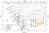 |
Fig. 1. Hertzprung–Russell diagram (HRD) of the BLOeM survey highlighting the BAF supergiant sample studied in this article with large star symbols colour-coded based on spectral type, as indicated by the legend. The three targets with the black circles indicate the only targets in this sample that have a clear indication of binarity: BLOeM 4-072, BLOeM 6-006, and BLOeM 6-008. The three targets with the black squares indicate targets that display a binary motion characteristic of long orbital periods: BLOeM 1-114, BLOeM 3-106, and BLOeM 8-001. Stellar parameters are determined using a calibration to spectral types by Paper I. Grey points show the entire BLOeM sample and stellar tracks from the extended grid of Schootemeijer et al. (2019) with mass-dependent overshooting (described in Appendix B of Hastings et al. 2021). The black marker with error bars on the left gives an indication of the typical uncertainties on the stellar parameters. The solid red line shows the magnitude limit imposed by the BLOeM survey target selection. The dashed red line is the Humphreys–Davidson (HD) limit, the cool part of which is shown as the revised-down limit in the SMC from Davies et al. (2018). |
The distribution of B- to F-type supergiants in the HRD reflects a long-standing puzzle in massive star evolution. The observed distribution of sources from the main sequence through to the F-type supergiant regime, only modified by the upper limit of the Humphreys–Davidson (HD) limit (Humphreys & Davidson 1979), is contrary to theoretical expectations and observed in all nearby star-forming galaxies (early references include Humphreys & Davidson 1979; Humphreys & McElroy 1984; Humphreys 1983; Fitzpatrick & Garmany 1990). Single-star evolutionary theory predicts a post-main-sequence gap in the HRD. This is because stars evolve rapidly towards the core helium burning phase and appear as red supergiants (RSG) or BAF-type supergiants after the end of the main sequence, with another gap between these two phases. The latter gap, sometimes referred to as the ‘Hertzsprung gap’, is indeed observed as a dearth of G-type supergiants (see previous references), while the issue of whether or not a BAF-type supergiant phase precedes or follows the RSG phase (i.e. the presence of blue loops in the HRD and the mass range within which these occur) depends sensitively on the mixing physics employed in the models. For a general discussion of these issues in the context of the SMC/LMC see, for example, Lennon et al. (2010), Schootemeijer et al. (2019, 2021) and Georgy et al. (2021). Complicating the picture further, most massive stars are born in binary or multiple systems that undergo interaction with a companion during their lifetime (Sana et al. 2012), leading to more complicated evolutionary scenarios. In this context, the stars found within the gap at the end of the main sequence may consist of post-interaction binaries, possibly hosting stripped stars or black holes, or perhaps they are even the results of stellar mergers (de Mink et al. 2014; Langer et al. 2020; Menon et al. 2024; Götberg et al. 2018; Villaseñor et al. 2023; Wang et al. 2024).
From an observational perspective, the stellar properties – in particular CNO abundances (Trundle & Lennon 2005; Trundle et al. 2007; Crowther et al. 2006; Weßmayer et al. 2022) and pulsation properties (Saio et al. 2013; Kraus et al. 2015; Bowman et al. 2019; Sánchez Arias et al. 2023; Ma et al. 2024) – are diagnostics that are used to assign evolutionary status. Such diagnostics are able to distinguish between core hydrogen burning (i.e. main sequence) stars with abundances dictated by mass loss and/or mixing, core-helium-burning stars whose properties are consistent with pre- or post-RSG evolution, mass transfer products in a binary system, and stellar mergers. However, given the importance of binary evolution in massive stars, critical information is provided by their multiplicity properties, which, when compared to other evolutionary stages, is particularly insightful for defining evolutionary histories. For example, an absence of blue supergiants with orbital separations too short to fit a RSG star could be interpreted as evidence for blue loops, since this phase would remove all but the longest period companions (Stothers & Lloyd Evans 1970). Furthermore, McEvoy et al. (2015) studied 52 B-type supergiants in the 30 Doradus region of the LMC, finding that the 18 binaries in this sample are mostly located at spectral types earlier than about B2; moreover, they speculated that the hotter sample constituted main-sequence stars, the cooler single stars being core-helium-burning (see their Fig. 4). A single cool binary in that sample was discovered to have a stripped star primary (Villaseñor et al. 2023).
The BLOeM data for the BAF supergiants therefore provide a unique opportunity for a systematic multiplicity study of late-B to F-type supergiants. This is a demographic that is relatively unexplored, as most spectroscopic monitoring studies of this group focused on a small number of the most luminous late-B- and A-type supergiants, the α Cygni variables (Parthasarathy & Lambert 1987; Rosendhal & Wegner 1970; Kaufer et al. 1997). This class of object displays radial-velocity (RV) variations caused by radial pulsations on timescales of days and typical amplitudes of 10–20 km s−1 that are capable of masking and/or mimicking binary motion. Burki & Mayor (1983) studied 45 F-type supergiants and found a binary fraction of 18%, albeit all but a few were judged to have periods longer than their five-year time baseline.
In this work, we used multi-epoch spectroscopic observations taken as part of the BLOeM campaign to investigate the variability of 128 BAF supergiant stars in the SMC. The sample selection is described in Sect. 2, and our methodology of determining multi-epoch RV time series is described in Sect. 3. The results are presented in Sect. 4, where we identify candidate binary systems and perform a multiplicity analysis based on the determined RV time series. This is discussed in Sect. 5, and our main conclusions are presented in Sect. 6.
2. Sample and observations
The BLOeM campaign is implemented on the Very Large Telescope (VLT) with the Fibre Large Array Multi Element Spectrograph (FLAMES; Pasquini et al. 2002). Briefly, it is used to observe ∼1000 massive stars distributed between eight FLAMES fields at different locations throughout the SMC using the LR02 grating, which covers the 3960–4570 Å wavelength range with a spectral resolving power (R) of 6200. Figure 2 shows the spatial distribution of the BAF supergiants throughout the SMC on a density map from the Gaia DR3 source catalogue (Gaia Collaboration 2023), while the number of sources per spectral subtype are shown in Table 1. Within the eight BLOeM fields there are typically 16 BAF supergiants per field. Field 3 has the most, at 26, followed by Field 8 with 22. As noted, while the full survey is delivering 25 epochs over two years, the currently available nine epochs were obtained over roughly 30–65 days depending on field number1.
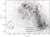 |
Fig. 2. Spatial location of the BAF-type supergiant sample in the SMC, overlaid on the density map of the Gaia DR3 source catalogue (G < 19 mag). Spectral types of the targets are colour-coded as indicated. Black circles mark the locations of the eight BLOeM fields. |
Number of targets and median peak-to-peak RV measurements (Δvmed) as a function of spectral sub-type for the BAF supergiants.
Data reduction and processing is described in Paper I; we note here that we used the cosmic-ray cleaned, merged, and normalised spectra in the present analysis. While most sources have spectra for all nine epochs, a few sources have fewer spectra, as noted in Table B.3. The median signal-to-noise ratio (S/N) of the individual spectra is 70, with an inter-quartile range of 40. In addition to the quality-control checks performed on the sample from Paper I, we performed some further comparisons with well-known stellar catalogues including Gaia Cepheid catalogues (Clementini et al. 2019; Ripepi et al. 2023), finding that BLOeM 5-005 is the classical Cepheid SV* HV 1954. Cepheid variables display large intrinsic variability, confirmed here in our RV measurements; therefore, we exclude this star from our discussion of the sample properties.
Table 1 and Fig. 1 demonstrate that the sample is dominated by later B-type and A-type supergiants; the B8–A7 stars comprise ∼75% of the sample and have a mass range of roughly6–26 M⊙, the bulk of which have masses below ∼13 M⊙. In this estimate, we assumed that the source masses are those implied by the evolutionary tracks. As expected, there are no sources above the HD limit, although a few sources are quite close to that boundary.
3. Methodology
Detecting binary motion for BAF supergiant stars is a more challenging task than doing so for earlier spectral types in that the expected periods are long, and, hence, the RV variations are small. As an indication, the minimum period possible for a mass ratio (q) of q = 0.5 for the range of parameters indicated in the HRD are between roughly 8 and 350 days, or 80 and 30 km s−1 in semi-amplitude velocity (for circular orbits). Adopting q = 0.1 changes the period range to 6–260 days and the semi-amplitude velocity range to 20–8 km s−1 (see Sect. 4.3 for further discussion). As these observations span 30–65 days and long-period binary systems are likely eccentric, we expect the majority of the detected binaries to exhibit rather small velocity variations. Accordingly, in our RV analysis we pay particular attention to precision and potential systematic errors.
We adopted the cross-correlation approach to measure RVs, which is well suited to stars with many lines, as is the case for the bulk of our sample. The precision improves as  , where N is the number of detectable lines. Figure 3 illustrates the significant change in morphology and line density across the spectral types considered here. We found that for some stars there is a small (∼ a few km s−1) instrumental shift between different spectral regions. Therefore, we restricted the cross-correlation to 4360–4560 Å (indicated by two dashed lines in Fig. 3) to ensure we used a common wavelength region for all stars. This mitigates possible systematic errors in the wavelength solution, but it is sufficiently wide to include enough strong lines in the earliest spectral types. Measurement of the RVs consists of two distinct parts: (i) determination of the relative RVs between separated observations; and (ii) determination of the zero point of the RV scale for each star.
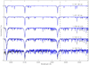 |
Fig. 3. A montage of BAF supergiant star spectra from BLOeM (in black) and best matching theoretical template spectra (blue) from CMFGEN/ATLAS model grids (see text). BLOeM IDs and spectral types are noted above each spectrum. Template spectra were used to determine an absolute RV scale, and one can see good agreement between line positions and strengths of the templates with the data. The vertical dashed lines indicate the spectral region that was used to derive the cross-correlation functions (CCFs) for all sources. We highlight the slight mismatch of the continuum for the F supergiant, BLOeM 1-102. For cool stars, the automatic continuum placement is more difficult due to the line density of the spectra; however, the CCFs are not impacted by this offset as we use normalised CCFs, such that the mean signal is subtracted from each spectrum before cross-correlation. We note that the A–F supergiant line spectra are dominated by Fe II and Fe I lines (for line lists, see Venn 1995, 1999). |
Zero points are determined using low-metallicity (Z) grids of CMFGEN models for B5–A supergiants covering 7250–14 500 K in effective temperature, a log g range of 1.0–2.5, and 1/5 and 1/10 solar metallicity levels (Garcia et al., private communication). This was supplemented with a low-Z (1/5 solar) ATLAS9 grid for the F stars (Howarth 2011), as important opacity sources for the cooler objects are currently not implemented in the CMFGEN grid. Important caveats include that the combined grid of models has a fixed Z and a fixed microturbulence value of either 5 or 10 km s−1. Hence, these grids do not provide tailored fits, but they are sufficient for RV determination. We find that RV zero points depend slightly on the choice of model template; because of this we cross-correlated each spectrum against all the models to find the best-matching template. We emphasise that the objective here is not to find definitive stellar parameters (given the caveats above) but to find the model in our pre-defined grid that best matches the line spectrum of each star. Nevertheless, the effective temperatures derived from the best matching template are in good agreement with those derived from spectral type calibrations from Paper I and are listed in Table B.3. For consistency, we also list new values of the stellar luminosity assuming a mean extinction for the SMC from Gordon et al. (2024). An inspection of Fig. 3, which shows some typical template matches, confirms that the cross-correlation regions are well modelled by the CMFGEN/ATLAS9 spectra.
Relative RV shifts among the nine epochs were determined by cross-correlating the normalised spectra against each other. We then formed an observational template spectrum by co-adding the separate exposures, taking care to use appropriate weights according to their respective S/N, and this was then cross-correlated against the model template to determine the RV zero-point offset for the data set. Cross-correlation uncertainties were calculated following Zucker (2003), with some minor modifications. Further details of this and the cross-correlation process are provided in Appendix A.
The derived RVs and their uncertainties are listed in Table B.2 (available in full via CDS), which shows that measured uncertainties can be as low as ∼0.1 km s−1 with a median value of 0.5 km s−1. Consequently, it is important to have a clear understanding of the likely systematic errors that might be present in the data. Plotting measured RVs as a function of time for stars grouped by their field number revealed correlations, which are an indication that small common velocity or pixel offsets exist between epochs for each field (see Fig. B.1). As discussed in more detail in Appendix B, we defined a subset of sources for each field that were most strongly correlated, and by implication had RV variations below the limit of the correlated errors. By assuming these sources have a constant RV, we computed median RV deviations at each epoch across all sources in each field. These corrections were applied iteratively to the measured data, with a few iterations typically sufficient to achieve convergence. These final RV corrections are listed in Table B.1 and are applied to the measured values for all sources in the present analysis and the subsequent discussion. We note that a corollary to Table B.2 is that there is an as-yet undetermined RV zero-point systematic uncertainty to the absolute RVs of the order of 1–2 km s−1.
Further insight into the nature of the RV variability of the sample was obtained by computing some simple statistics for each source with results obtained from the corrected values summarised in Table B.3. In the subsequent sections we examine the mean RV and its standard deviation, the peak-to-peak RV variability (Δv, which is the difference between the maximum and minimum RVs), and the median error of the individual RV measurement errors. In addition, for each target we determined the significance of each pair of measurements using the equation
 (1)
(1)
where vi, j and σi, j are the RVs and their associated uncertainties at epochs i or j. As discussed by Sana et al. (2013a); Dunstall et al. (2015) and Patrick et al. (2019), this quantity is often used in conjunction with a threshold condition,
 (2)
(2)
where Δvlim was chosen to reject possible intrinsic RV variations that are not caused by orbital motion but, for example, are the result of stellar activity such as pulsation.
4. Results
A key discovery from the analyses of the observed spectra is the absence of large-scale Δv values for the entire BAF supergiant stars within the BLOeM sample. Figure 4 shows the distribution of Δv values as a function of spectral type, and Table 1 shows the median values as a function of spectral subtype.
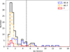 |
Fig. 4. Histogram of peak-to-peak radial-velocity (RV) measurements (Δv) for the BAF supergiant sample. Different colours highlight the sub-samples as indicated in the panel. The dashed black line is the chosen threshold for binarity in the multiplicity analysis. |
4.1. Binary detection
Equation (1) together with an appropriate choice of the threshold indicated in Eq. (2) are typically used as criteria for the detection of binary candidates. For example, Sana et al. (2013a) adopted Δvlim = 20 km s−1 and σi, j = 4 for O-type stars in the 30 Doradus region of the LMC, while Dunstall et al. (2015) adopted 16 km s−1 and σi, j = 4 for B-type stars in the same region. The latter choice reflects a somewhat better precision level on RV measurements and smaller expected contribution from intrinsic RV variability (e.g. de Burgos et al. 2020). For O-hypergiants and WNh stars, Clark et al. (2023) selected a larger limit of 30 km s−1 while maintaining the σi, j = 4.
The choice of σi, j (see Eq. (1)) is motivated by the sample size – to exclude false positives – and the level of significance attached to the detection. For the BAF supergiant sample, small uncertainties on the v measurements mean that the choice of the σi, j threshold does not affect the results significantly. Therefore we selected σi, j = 4. Consequently, there are 23 sources (excluding the Cepheid) that meet this criteria.
The choice of the Δvlim threshold (see Eq. (2)) is driven by the need to exclude intrinsic RV variability as a result of pulsations or other physical mechanisms. For example, intrinsic RV variability of O-type supergiant stars was found to be significant by Fullerton et al. (1996), and the vast majority of studied B-type supergiants are observed to be intrinsically variable (see Bowman et al. 2019; de Burgos et al. 2020). However, RV variability is rather modest for most RSGs (Josselin & Plez 2007; Patrick et al. 2019; Dorda & Patrick 2021). From an examination of Fig. 4, adopting even the lowest of the RV thresholds from the aforementioned previous studies in the OB-star regime results in the detection of no binaries in the BAF supergiant sample. In an attempt to define a physically meaningful threshold for binary detection, Sana et al. (2013b) assessed the distribution of Δvlim as a function of stars that meet the threshold (see Fig. 9). These authors argued that their results displayed a kink at ∼20 km s−1, which they attributed physical meaning and subsequently selected this as the threshold for binarity. This prompted other authors to look for similar features, which are typically not found (for examples in this series, see Fig. 5 of Villaseñor et al. 2025 or Fig. 5 of Britavskiy et al. 2025). We analysed this distribution for the BAF supergiant stars (and B5–9 and AF stars individually) and did not find a clear indication for a transition between intrinsic and orbital variability. In lieu of a physically motivated choice of Δvlim, we selected Δvlim = 5 km s−1 based on the distribution of observed Δv values from the BAF supergiants. Figure 4 demonstrates that a choice of Δvlim = 5 km s−1 is a reasonable value to mitigate intrinsic variability. We acknowledge that this limit is unsatisfactory. To address this further may require full binary solutions for the candidates detected here but this is clearly outside the scope of the current article. Similarly, in tandem, photometric constraints on intrinsic variability could potentially be used on a star-by-star basis to determine a physically motivated threshold Δvlim.
Based on these criteria (i.e. adopting Δvlim = 5 km s−1 and σi, j = 4), only 13 of the sample, or 10% of the total BAF supergiant sample, meet both RV variability criteria to be classified as candidate binaries. These stars are marked with the ‘var’ flag in Table B.3. Splitting the sample by spectral type, we find the B5–9 type stars have an observed binary fraction of 25 ± 6 (12/47)2. For the A-type supergiants we find 4 ± 2% (3/69) and for the F-type supergiants we find 8 ± 8% (1/12). The lone binary candidate F-type supergiant BLOeM 6-006 is also a borderline case. Further dissecting the B-type supergiants reveals no significant evidence of a trend as a function of spectral sub-type. Combining the AF stars, we find 5 ± 2% (4/81).
For the B5–9 supergiants, it is likely that the specified 5 km s−1 threshold for binarity is significantly contaminated by intrinsic RV variability (see Sect. 4.2). The AF-type supergiants appear to be less affected by intrinsic variability; therefore, in the remainder of this article we split the sample to consider the B5–9 and the AF supergiants separately. If we assume a more stringent limit of 10 km s−1 for both samples in attempt to minimise the effects of intrinsic RV variability, we find an observed binary fraction of 10 ± 4% and 0% for the B5–9 and AF samples, respectively.
As a result of the sampling of observed epochs, the baseline of observation, and the uncertainties associated with the RV measurements, the observed binary fraction should be considered a lower limit on the intrinsic binary fraction. We accounted for these observational biases by simulating a population of binary systems using the Monte Carlo method developed by Sana et al. (2012, 2013b). Table 2 displays the ranges and assumed distributions of the orbital parameters that are used to determine the bias-corrected multiplicity fraction. The orbital-period distribution is assumed given the result of Sana et al. (2025). The flat q distribution is based on results from Shenar et al. (2022a) and Patrick et al. (2022). The mass function of the sample was tested using the stellar parameters determined in Paper I and found to be consistent with a power law of exponent γ = −2.35. This approach results in a bias-corrected multiplicity fraction of ∼30% for the BAF supergiant sample. However, as noted above we consider that the results for the B5–9 sub-sample are impacted by intrinsic variability, specifically by the prevalence of the α Cygni variables (see Sect. 4.2). Because of this, we split the sample at A0 and redetermined the statistics by taking into account the fact that the AF stars are significantly larger than their B5–9 counterparts by considering orbital periods in the 1.25 < log P/d[dex] < 3.5 range (see Sect. 4.3). This results in a bias-corrected multiplicity fraction of 8 % for the AF-type supergiants, which is thus less affected by intrinsic RV variability. In addition, for the B5–9 sub-sample we performed the bias correction simulations for the observational limit of 10 km s−1, which results in an intrinsic binary fraction of 18
 % for the B5–9 supergiants.
Range of orbital parameters and their assumed distributions considered in the bias correction calculations.
The choice of the assumed orbital property distributions and their uncertainties clearly has an impact on the final quoted binary detection statistics. Our chosen distributions largely represent those appropriate for unevolved stars of similar masses and assume no binary evolution; this ensures consistency with other studies in the BLOeM campaign. If the population of BAF supergiants is dominated by binary interaction products, the bias-corrected multiplicity fraction is likely to be inaccurate. To assess the impact of this, we repeated the bias-correction simulations with a range of underlying distributions including, for example, a split q-distribution (Moe & Di Stefano 2017), which favours more low-q systems. This results in a bias-corrected multiplicity fraction of 8 % for the AF-type supergiants, which is in good agreement with the above results. This gives us confidence that the final results are robust to the exact choices of the orbital parameter distributions.
4.2. Constraints on intrinsic variability from visual inspection
The size and spectral coverage of the BAF supergiant sample combined with the BLOeM campaign design – and the relative lack of RV variability found in the previous section – provides an excellent opportunity to characterise the intrinsic variability of BAF supergiants in the SMC. The distribution of Δv values for the BAF supergiant sample as a function of spectral type (see Fig. 4) clearly shows the scarcity of large Δv values at all spectral types. The Δv measurements cluster around a value of 1 km s−1 with a sharp drop beyond 2 km s−1, and perhaps a small over-density near 4–6 km s−1, mostly due to the B-type stars. In particular, for the AF supergiant stars there are no Δv values larger than ∼6 km s−1. Table 1 shows the typical Δv values as a function of spectral type.
To investigate the intrinsic RV variability, Fig. 5 shows Δv as a function of stellar radius together with the B3 supergiants from Britavskiy et al. (2025). The latter are likely to be post-main-sequence stars as discussed by Britavskiy et al. (2025) and are expected to display similar RV properties to the B5–9 stars. The sizes of the points in Fig. 5 are determined by the significance of the Δv measurement, which is defined as Δv/σΔv. This distribution reveals a clustering of points that suggests a trend of decreasing Δv with increasing radius (and, by inference, with decreasing effective temperature). This trend is driven primarily by the improving precision as one moves to cooler stars that have more spectral lines. Moreover, many of the B3 and B5 supergiant stars have lines broadened by rotation, which leads to larger RV uncertainties at the hot end of the distribution. However, the stars with the largest Δv/σΔv are discrepant from this general distribution.
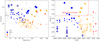 |
Fig. 5. Left panel: Peak-to-peak RV (Δv) as a function of stellar radius for the BAF supergiants and the B3 supergiants of Britavskiy et al. (2025). Radii were determined using effective temperatures and luminosities from Table B.3. The sizes of the symbols in both panels are determined by Δv/σΔv. Black circles mark stars of the cohort of variable late-B-type bright giants. Right panel: HRD for BAF supergiant sample using stellar parameters listed in Table B.3; symbols have the same meaning as in the left panel. We note that the sources with largest Δv/σΔv tend to be the most luminous and hottest stars. |
In the right panel of Fig. 5, we see that the stars with the most significant RV variability and largest Δv values are among the most luminous BAF supergiants. Kaufer et al. (1997) presented a detailed analysis of long-term monitoring data for photospheric lines of six luminous supergiants in the B7–A2 spectral domain (i.e. α Cygni variables that include α Cyg and β Ori) and found significant RV variability with Δv values in a range from 15 to 20 km s−1. These authors tentatively attributed this variability to non-radial gravity-mode pulsations, though this is debated (see e.g. Saio et al. 2013).
For the most luminous stars that occupy a similar region in the HRD to the sample discussed by Kaufer et al. (1997), it seems likely that we are detecting α Cygni variability due to pulsations rather than orbital motion. Here, we assigned seven stars an α Cygni flag (shown in Table B.3) based on their high luminosity and significant RV variability. It is interesting that there is a lack of strongly variable, α Cygni-like sources among the AF supergiants. This is perhaps indicative of their differing luminosity-to-mass ratios, and/or perhaps hints at a different evolutionary path. While we assigned only seven stars the α Cygni designation, it is likely that our selection missed a significant number of candidates at lower luminosities.
To test whether the observed RV variability is a result of orbital motion or pulsation, we visually checked for long-term trends in the RV time series. Figure 6 illustrates three examples of RV variability that are clearly subject to variations on short timescales (days) that would be consistent with the findings of Kaufer et al. (1997) for pulsations3. The fourth panel in that figure, for BLOeM 6-008, is an example of a potential binary showing a long-term trend with clearly smaller short timescale variability.
These four sources have high luminosities and, therefore, large radii resulting in minimum periods for q = 0.5 of 100 days or more. Fitting orbital solutions to the RV time-series data using the program RVFIT (Iglesias-Marzoa et al. 2015) yielded only spurious solutions for the first three sources. The solution for BLOeM 6-008 indicates a period of ∼180 days. The fit is poorly constrained, which indicates that the full 25-epoch coverage of the BLOeM campaign is required to further our knowledge of this candidate binary system. In fact, only two other stars in the var category (see Table B.3) exhibit RV variability that can be considered binary motion, namely BLOeM 4-072 (B9 Ia) and 6-006 (F2:). Time-series RVs for all 14 sources flagged as var in Table B.3 are presented in Appendix C. Visual inspection of the full sample reveals only three additional sources that may be compatible with a long-term trend: BLOeM 1-114, 3-106, and 8-001. These objects are flagged as ‘LP’ in Table B.3. Running RVFIT for all these systems resulted in similarly poor results to those for the var sample.
In addition, based on further inspection of Fig. 5, we highlight a second cohort based on their similar Δv values, effective temperatures, and luminosities. This grouping consists of late B-type bright giants. The stars that we consider members of this cohort are BLOeM 3-092, 3-102, 4-004, 5-086, 6-007, and 6-097. These stars are highlighted with black circles in Fig. 5. Interestingly, all six objects appear to have significant rotational broadening.
In summary, it is clear that the observed and bias-corrected multiplicity fractions of BAF supergiant stars are seriously compromised by the intrinsic variability of the most luminous systems. The true binary fraction is significantly smaller.
4.3. Constraints on detectable orbital configurations
The result of the low detected binary fraction for the BAF supergiant stars naturally raises the question of how sensitive the BLOeM survey is when it comes to detecting binary systems in the appropriate orbital period range. To assess this, we simulated populations of binary systems using the parameters given in Table 2. In these simulations, each system is assigned a random inclination angle with respect to the observer and we generated RVs with a baseline, sampling, and uncertainties typical of the BLOeM observations. We then tested whether or not each system would meet the criteria to be classed as a binary, similarly to how we applied our multiplicity analysis described in Sect. 4.1 (i.e. Δv = 5 km s−1 and σ = 4). Figure 7 shows two findings from this analysis for the P-q parameter space, whereby the solid contour lines in the left panel indicate the probability of detection from 10 000 binary simulations per grid point. The solid lines in the right panel show constant semi-amplitude velocity values from the simulated systems. Also shown is the minimum period possible for three stars – BLOeM 3-009 (B5 II), 4-075 (A0 I), and 8-089 (F2:) – for a range of q values. Stellar parameters are taken from Table B.3, and estimates of stellar masses are taken from the evolutionary tracks. We note that these three stars are clustered around the median of the luminosity distribution (with log(L/L⊙) in the range 4.3–4.5) and radii typical of their spectral types. Hence, the constraints illustrated in Fig. 7 and discussed below are even more stringent for the more luminous stars.
In the left panel of Fig. 7, it is apparent that the observations are sensitive to orbital periods up to hundreds of days, but sensitivity falls off significantly beyond 1000 days. For example, for the B5 stars, binary systems would be detected in the 5 < P < 100 days range at above the 90% confidence level for the full range of q > 0.1. In contrast, for the 12 F-type supergiant stars, the parameter space of orbital configurations that reach the 90% level of detection probability is very small, and, as such, our true detection probability for the F-type stars is significantly smaller than that of the B-type stars. As the assumed log P and q distributions are roughly flat in nature (for q > 0.1), the area to the right of the dashed lines in Fig. 7 illustrates the true detection probability for each target. As a representative example, the observations are around twice as likely to be able to detect binary motion for a B5 star than an A0 star. Taken together, the two panels of Fig. 7 clearly shows that binaries with orbital periods within 5 < P < 100 days and having q > 0.1 should produce a strong signal within the current observational setup, but these are not observed.
Beyond an orbital period of around 300 days, a significant fraction of companions go undetected based on orbital motion. While the bias-correction simulations account for such systems in the statistics determined in Sect. 4.1, it is important to describe the types of systems that are undetected in the current observational setup. The UVIT survey allows us to fill in such systems at < ∼5 M⊙ (see Sect. 4.4) but the BAF sample could still harbour undetected long-period companions. This includes main-sequence companions as well as binary-interaction products such as stripped stars and compact companion systems.
4.4. Binary systems detected via UV excess
Hota et al. (2024) published a far-ultraviolet (FUV) catalogue (Hota, private communication) for the SMC using data from the Ultra Violet Imaging Telescope (UVIT) onboard AstroSat, and all but a handful of BLOeM targets overlap with its footprint. Cross-matching with that catalogue using a 0.5″ matching radius, we find 754 BLOeM sources with FUV magnitudes. Figure 8 displays the matches in an optical-FUV colour-magnitude diagram (specifically Bp − Rp versus FUV). Only three BAF sources are outliers in this diagram (BLOeM 5-109 (A7 Iab), BLOeM 6-008 (A2 Ia), and BLOeM 4-006 (F2:). We assume that these sources with UV excesses are the result of a hot companion. The FUV magnitudes of these sources are consistent with main-sequence companions in the 15–20 M⊙ mass range (see Fig. 5 of Patrick et al. 2022), which may make the BAF supergiant the less massive component of possible binary systems. However, the detection limit of the Hota et al. (2024) catalogue corresponds to a main-sequence mass of around 5 M⊙, which may explain the low overall detection rate. We note that BLOeM 6-008 is also a source that exhibits a long-term trend in its RV time series, as shown in Fig. 6. BLOeM 4-006 was denoted as a possible SB2 system (i.e. ‘SB2?’ in Paper I), however its RV time series is effectively constant within the errors; hence, this may be either a chance alignment or a very long-period system. BLOeM 5-109 also exhibits an RV time series that is constant within its errors. In addition to these three sources, the two B[e] supergiant stars that are in the BLOeM sample are also outliers (also shown in Fig. 8).
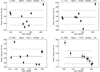 |
Fig. 6. Radial-velocity (RV) time series for four of the targets that display RV variability above the chosen thresholds (see text), with spectral types of A Ia (BLOeM 1-051), B9 Ia (1-112), B8 Ia (2-093), and A2 Ia (6-008). Identifications are listed in the panel headings, as are the mean RVs and their standard deviations, which are indicated in each panel by solid and dashed lines, respectively. We note that only 6-008 displays evidence of a long-term RV trend that might be a signature of binary motion. Due to their large radii, all of these stars have minimum periods of ∼100 days or more. |
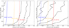 |
Fig. 7. Left: Orbital period shown against mass ratio (q) for simulated binary systems in the orbital period ranges that were used to correct for our observational biases. Solid black contour lines show the probability of detection at the 99, 90, 50, and 10% levels given the temporal baseline and typical uncertainties of the BLOeM data, where each grid point is the median of 10 000 simulated systems. The detection criteria used in these simulations are matched to those of the observations (i.e. Δv = 5 km s−1 and σ = 4). The dashed coloured lines show the minimum allowed orbital period for three representative examples as a function of the mass ratio of the system. Right: Same simulations where the solid contour lines now show lines of constant semi-amplitude velocity on the 150, 100, 50, 25, and 10 km s−1 levels. |
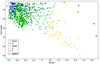 |
Fig. 8. Colour-magnitude diagram using 754 BLOeM sources found in the UVIT FUV catalogue (Hota et al. 2024), colour-coded by spectral type. The FUV magnitude was obtained with the F172M filter, while the BP − RP colour is from GaiaBp and Rp filters. The five outliers described in Sect. 4.4 are flagged with black circles. |
A cross-match with the yellow supergiants (YSGs) in O’Grady et al. (2024), who searched for UV excesses from Swift data, resulted in four stars in common: BLOeM 6-009, 6-002, 6-052, and 5-109. Of these, both BLOeM 6-009 and 6-052 are found to have UVIT FUV magnitudes commensurate with their spectral types, whereas BLOeM 6-002 is not recovered, despite it being within the UVIT footprint. Given the smaller point spread function (PSF) of UVIT compared to Swift – a full width at half maximum of 1″ versus 2.5″ – it is possible the discrepancy is a consequence of the larger PSF of Swift detecting a nearby star. We note that BLOeM 5-109 is the only source detected in the uvm2 filter from the Swift data; accordingly, we only flag the UVIT UV excess sources in Table B.3.
5. Discussion
5.1. Direct evolution from the main sequence
A general conclusion of our analysis (see Sect. 4.3) is that there appears to be a ‘period gap’ up to ∼102 days in the BAF supergiant sample. Specifically, there is a dearth of ‘short’-period systems with mass ratios above 0.1. An important implication of this finding is that it provides constraints on the evolution of the system evolving redwards across the HRD. To address this issue, we compare our sample with that of other BLOeM studies: Britavskiy et al. (2025) finds a bias-corrected multiplicity fraction of 40 ± 4% for the B0–3 supergiants, while Villaseñor et al. (2025) finds 80 ± 8% for the B0–2 giants and dwarfs, and Sana et al. (2025) finds  % for the O-type stars.
To test the agreement between the multiplicity fraction of the different BLOeM samples, we simulated populations of binary systems with ranges of orbital configurations and underlying distributions following Table 2 to account for the differences in the allowed orbital configurations for the BAF supergiant sample, which we split into two bins: the B5–9 supergiants and the AF supergiants. We created simulated observations to match the sample size, baseline, and uncertainties of each of the two sub-samples. Figure 9 shows a comparison between the observed results (solid black lines) and simulations of populations of binary systems whose bias-corrected multiplicity statistics are determined on the main sequence by Villaseñor et al. (2025) and evolved to match the different samples (red dashed lines). One would expect that the black and the red dashed lines to overlap significantly, particularly at large Δvlim, if the simulations agreed with the observations. However, these comparisons demonstrate that the simulated population of binary systems evolved from the main-sequence drastically over-predicts the level of high-amplitude RV variability caused by binarity. To illustrate this further, we applied the same binary threshold criteria to the simulated data, Δvlim = 5 km s−1 and σi, j = 4, to predict an observed binary fraction for the AF supergiant stars of 40 %. This is clearly significantly larger than the observed binary fraction of 5 ± 2%. This quantitatively demonstrates that the origin of the BAF supergiants cannot be explained by a direct evolution from the main sequence. Here, we restrict the discussion to the AF supergiants because of the uncertain contribution from intrinsic RV variability for the B5–9 sample, although one can see from the left panel of Fig. 9 that even without accounting for intrinsic RV variability, the simulations over-predict the observed multiplicity fraction. Altering the simulations by experimenting with different values for the underlying q-distribution to favour more low-q systems changes the appearance of the red lines in Fig. 9, but it does not alter the key result that the simulations cannot explain the absence of large-amplitude orbital motion.
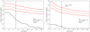 |
Fig. 9. Fraction of detected binarity as function of Δvlim. The solid black line in the left panel shows the B5–9 supergiants, and the right panel is the same, except for AF supergiants. The dashed red lines show the simulated binary fraction assuming an intrinsic binary fraction on the main sequence of 75 ± 10% – to roughly match that of Villaseñor et al. (2025) – which was evolved to remove binary systems that would have since interacted based on the current sizes of the stars. The solid red lines show the bounds of the assumed uncertainty on the intrinsic multiplicity fraction. |
As noted in the introduction, Burki & Mayor (1983) found a binary fraction for F-type supergiants of ∼18% in the Milky Way. However, their observing window was five years, such that all but a few of those binaries have periods in excess of this time span, and all have RV variations less than 5–10 km s−1 (see their Fig. 2a and Table 7). Hence, given our current observational baseline, it is unlikely that we would have detected any of their sources as RV variable. We conclude that our results are consistent with Burki & Mayor (1983) given the differences in baseline and, hence, orbital period range. An important corollary to that work is that such long periods (in excess of five years) and small RV amplitudes imply a very low binary mass function, probably indicating solar or sub-solar companions.
5.2. Comparison with RSGs
Assuming single-star evolution, our samples are either evolving towards the RSG stage or have previously been RSGs. Patrick et al. (2022) studied the multiplicity statistics of RSGs (∼4500–3800 K) in the SMC with UV photometry and found a multiplicity fraction of 18 ± 4% for orbital periods approximately in the range of 3 < log P[days]< 8 and q in the range with 0.3 < q < 1.0. They also argued, based on a comparison with multiplicity results from B-type stars in the LMC (Dunstall et al. 2015), that the orbital period distribution drops drastically around log P[days]> 3.5. The q-distribution that was assumed by Patrick et al. (2022) is the same as used here (i.e. flat), which means that we can account for the differences in the q range considered. Taking this into account results in a bias-corrected multiplicity fraction of the AF supergiant stars of 9%. This is smaller than the multiplicity fraction for the RSG population, but compatible at the 3-σ level. Here, as in the previous subsection, we restrict the discussion to the AF supergiant stars because of the uncertain contribution from variability for the B5–9 sample.
If the inference that the orbital distribution falls for periods longer than log P ∼ 3.5 is correct, this can be interpreted as evidence that the multiplicity properties of the AF supergiant stars are inconsistent with being pre-RSG objects as their binary statistics are incompatible with undergoing blue loops in the HRD. The lack of BAF supergiant sources with a FUV excess would also be consistent with this scenario.
5.3. Binary interaction products
Having mainly considered single stellar evolutionary pathways for the origin of the BAF supergiant sample so far, we turn our attention to potential binary pathways. For example, sources such as the ‘puffed-up’ stripped star plus OB-star system VFTS 291 (Villaseñor et al. 2023, spectral type B5 Ib-II), which has an orbital period of 108 days and semi-amplitude RV of ∼94 km s−1, are clearly not present in the BAF supergiant sample. In addition, while the current spectral type of the stripped star ‘primaries’ of systems such as LB-1 and HR 6819 (Shenar et al. 2020; Bodensteiner et al. 2020, periods of ∼79 days and ∼40 days) are early B-type stars, their precursors would likely have been in the effective temperature range of BAF stars. Given the expected low mass of such ‘primaries’ (i.e. the optically brightest component), and relatively high mass of the secondaries (i.e. q > 1.0), one might expect that the detection probability of such systems would be high, as implied by Fig. 7. On the other hand, the expected number of such systems depends on the expected lifetime of this phase. Dutta & Klencki (2024) discussed the dependence on mass, luminosity, and metallicity on such short-lived post-interaction evolutionary phases. From binary population synthesis they argued that as many as 0.5–0.7% of systems with log L/L⊙ > 3.7 may be puffed up stars. One might therefore expect only a handful of such systems in the ∼1000 BLOeM sources, the bulk of these among the more numerous O- and early-B-type stars.
Another important product of binary evolution are OB+BH binaries, which are expected to comprise ∼5% of all OB-type stars in binaries (Langer et al. 2020). A small number of such systems have been identified observationally (Mahy et al. 2022; Shenar et al. 2022b). The LMC theoretical period distribution from Langer et al. (2020) has a significant fraction of systems with long periods – peaking at just over 100 days – and semi-amplitude velocities of as much as 50 km s−1. The lack of detection of such long-period compact companions is supporting evidence that the BAF supergiant sample cannot be explained by stars that have directly evolved from the main sequence.
Furthermore, the SMC hosts a large number of high-mass X-ray binaries (HMXBs), with the bulk of these, ∼70, being Be X-ray binaries (BeXRB) comprising late-O- to early-B-type primaries and orbital periods of a few tens to a few hundred days (McBride et al. 2008; Townsend et al. 2011; Coe & Kirk 2015; Haberl & Sturm 2016). Only one system, SMC X-1, has a blue supergiant donor star, Sk 160 (O9.7Ia+). The compact object in SMC X-1 is a neutron star. The range of primary spectral types among HMXBs in the SMC and mass functions implies q values in the range of ∼0.05 < q < 0.30, which is within our sensitivity range. To illustrate this, Fig. 7 displays detection probabilities for orbital configurations down to q = 0.05. This demonstrates that low-q systems remain detectable at the 90% detection level with orbital periods in the range 5 < P < 30 days. Therefore, we might expect to detect long-period BeXRB (or OB plus neutron star binaries) that have not yet undergone a common envelope phase. We note that synthesis of the BeXRB binary population in the SMC also contains a tail of longer periods than are detected currently (Vinciguerra et al. 2020). One might conclude, therefore, that the BeXRB population does not survive into this part of the HRD. Finally, the scarcity of binaries in the BAF supergiant population is consistent with predictions of stellar mergers, occurring either on the main sequence or in the RSG regime (Justham et al. 2014; Menon & Heger 2017; Schneider et al. 2024), which predict single-star products as blue supergiants in the BAF effective temperature range (Menon et al. 2024).
6. Summary and conclusions
In this work, we investigated the intrinsic RV variability and multiplicity properties of the supergiant stars ranging from spectral types B5 to F5 in the SMC. We find a dearth of short-period binary systems (5 < P < 100 days) for the BAF supergiants in the BLOeM campaign. Evidence for this is the significantly smaller observed and bias-corrected binary fractions for the BAF sample compared to that of main-sequence stars (Sana et al. 2025; Villaseñor et al. 2025) and the small peak-to-peak RV values (Δv) observed. This is in contrast to the study of the B0–3 supergiant stars in the BLOeM campaign that show large Δv, which is indicative of short-period binary systems. We find an observed multiplicity fraction of between 10 and 25% for the B5–9 supergiants, which is likely affected by intrinsic variability, such as pulsations (e.g. α Cygni variables). We find an observed multiplicity fraction of 5 ± 2% for the AF supergiant stars. Taking into account observational biases, we determine the intrinsic multiplicity fractions are less than 18% for the B5–9 supergiants and 8 % for the AF supergiants. We caution, however, that these results – particularly for the B5–9 sample – are likely significantly affected by uncorrected intrinsic RV variability, which if accounted for would result in smaller intrinsic multiplicity fractions. Our key conclusions are as follows:
-
We examined the evolutionary status of the BAF supergiants via a comparison with main-sequence stars in the BLOeM campaign from Villaseñor et al. (2025) and conclude that the BAF supergiant stars are inconsistent with a direct redward evolution from the main sequence. This suggests the BAF supergiants either were born as effectively single stars or are binary interaction products. We compare our results with multiplicity statistics for RSGs in the SMC and conclude that the AF supergiants are inconsistent with being pre- or post-RSG objects. While the origin of both groups of supergiants remains unclear, our results are able to rule out multiple evolutionary pathways.
-
By assessing the BLOeM spectra and RV time series of the detected binary systems, we can conclude that, remarkably, only a small fraction of stars display convincing orbital solutions. In addition, there are no systems where a definite orbital period can be determined. This suggests that the true multiplicity fraction of both the B5–9- and the AF-type supergiants is lower than 15%, but inconsistent with zero, based on UV-detected companions and indications of long orbital periods for a handful of systems.
Data availability
Tables B.1, B.2, and B.3 are available at the CDS via anonymous ftp to cdsarc.cds.unistra.fr (130.79.128.5) or via https://cdsarc.cds.unistra.fr/viz-bin/cat/J/A+A/698/A39
The exact baseline per field is detailed in the Appendix of Paper I.
The uncertainties for the percentages in this paragraph are determined using binomial statistics where the standard error is  .
.
Three additional sources with similar properties to these are are BLOeM 2-092, 4-072, and 8-010.
Acknowledgments
We thank Sipra Hota for kindly sharing the SMC UVIT catalogue prior to publication. LRP, FN. and FT acknowledge support by grants PID2019-105552RB-C41 and PID2022-137779OB-C41 funded by MCIN/AEI/10.13039/501100011033 by “ERDF A way of making Europe”. LRP acknowledges support from grant PID2022-140483NB-C22 funded by MCIN/AEI/10.13039/501100011033. TS acknowledges support by the Israel Science Foundation (ISF) under grant number 0603225041. The research leading to these results has received funding from the European Research Council (ERC) under the European Union’s Horizon 2020 research and innovation programme (grant agreement numbers 772225: MULTIPLES). DMB gratefully acknowledges support from UK Research and Innovation (UKRI) in the form of a Frontier Research grant under the UK government’s ERC Horizon Europe funding guarantee (SYMPHONY; grant number: EP/Y031059/1), and a Royal Society University Research Fellowship (grant number: URF\R1\231631). GGT is supported by the German Deutsche Forschungsgemeinschaft (DFG) under Project-ID 496854903 (SA4064/2-1, PI Sander). AACS is funded by the Deutsche Forschungsgemeinschaft (DFG, German Research Foundation) in the form of an Emmy Noether Research Group – Project-ID 445674056 (SA4064/1-1, PI Sander). GGT and AACS further acknowledges support from the Federal Ministry of Education and Research (BMBF) and the Baden-Württemberg Ministry of Science as part of the Excellence Strategy of the German Federal and State Governments. This paper benefited from discussions at the International Space Science Institute (ISSI) in Bern through ISSI International Team project 512 (Multiwavelength View on Massive Stars in the Era of Multimessenger Astronomy). DP acknowledges financial support by the Deutsches Zentrum für Luft und Raumfahrt (DLR) grant FKZ 50OR2005. JIV acknowledges support from the European Research Council for the ERC Advanced Grant 101054731. PAC is supported by the Science and Technology Facilities Council research grant ST/V000853/1 (PI. V. Dhillon). JSV is supported by Science and Technology Facilities Council funding under grant number ST/V000233/1. DFR is thankful for the support of the CAPES-Br and FAPERJ/DSC-10 (SEI-260003/001630/2023). This work has received funding from the European Research Council (ERC) under the European Union’s Horizon 2020 research and innovation programme (Grant agreement No. 945806) and is supported by the Deutsche Forschungsgemeinschaft (DFG, German Research Foundation) under Germany’s Excellence Strategy EXC 2181/1-390900948 (the Heidelberg STRUCTURES Excellence Cluster).
References
- Bodensteiner, J., Shenar, T., Mahy, L., et al. 2020, A&A, 641, A43 [NASA ADS] [CrossRef] [EDP Sciences] [Google Scholar]
- Bodensteiner, J., Shenar, T., Sana, H., et al. 2025, A&A, 698, A38 [NASA ADS] [CrossRef] [EDP Sciences] [Google Scholar]
- Bowman, D. M., Burssens, S., Pedersen, M. G., et al. 2019, Nat. Astron., 3, 760 [Google Scholar]
- Britavskiy, N., Mahy, L., Lennon, D. J., et al. 2025, A&A, 698, A40 [NASA ADS] [CrossRef] [EDP Sciences] [Google Scholar]
- Burki, G., & Mayor, M. 1983, A&A, 124, 256 [NASA ADS] [Google Scholar]
- Clark, J. S., Lohr, M. E., Najarro, F., Patrick, L. R., & Ritchie, B. W. 2023, MNRAS, 521, 4473 [NASA ADS] [CrossRef] [Google Scholar]
- Clementini, G., Ripepi, V., Molinaro, R., et al. 2019, A&A, 622, A60 [NASA ADS] [CrossRef] [EDP Sciences] [Google Scholar]
- Coe, M. J., & Kirk, J. 2015, MNRAS, 452, 969 [NASA ADS] [CrossRef] [Google Scholar]
- Crowther, P. A., Lennon, D. J., & Walborn, N. R. 2006, A&A, 446, 279 [NASA ADS] [CrossRef] [EDP Sciences] [Google Scholar]
- Davies, B., Crowther, P. A., & Beasor, E. R. 2018, MNRAS, 478, 3138 [NASA ADS] [CrossRef] [Google Scholar]
- de Burgos, A., Simon-Díaz, S., Lennon, D. J., et al. 2020, A&A, 643, A116 [NASA ADS] [CrossRef] [EDP Sciences] [Google Scholar]
- de Mink, S. E., Sana, H., Langer, N., Izzard, R. G., & Schneider, F. R. N. 2014, ApJ, 782, 7 [Google Scholar]
- Dorda, R., & Patrick, L. R. 2021, MNRAS, 502, 4890 [NASA ADS] [CrossRef] [Google Scholar]
- Dunstall, P. R., Dufton, P. L., Sana, H., et al. 2015, A&A, 580, A93 [NASA ADS] [CrossRef] [EDP Sciences] [Google Scholar]
- Dutta, D., & Klencki, J. 2024, A&A, 687, A215 [NASA ADS] [CrossRef] [EDP Sciences] [Google Scholar]
- Fitzpatrick, E. L., & Garmany, C. D. 1990, ApJ, 363, 119 [Google Scholar]
- Fullerton, A. W., Gies, D. R., & Bolton, C. T. 1996, ApJS, 103, 475 [NASA ADS] [CrossRef] [Google Scholar]
- Gaia Collaboration (Vallenari, A., et al.) 2023, A&A, 674, A1 [NASA ADS] [CrossRef] [EDP Sciences] [Google Scholar]
- Georgy, C., Saio, H., & Meynet, G. 2021, A&A, 650, A128 [NASA ADS] [CrossRef] [EDP Sciences] [Google Scholar]
- Gordon, K. D., Fitzpatrick, E. L., Massa, D., et al. 2024, ApJ, 970, 51 [Google Scholar]
- Götberg, Y., de Mink, S. E., Groh, J. H., et al. 2018, A&A, 615, A78 [NASA ADS] [CrossRef] [EDP Sciences] [Google Scholar]
- Haberl, F., & Sturm, R. 2016, A&A, 586, A81 [NASA ADS] [CrossRef] [EDP Sciences] [Google Scholar]
- Hastings, B., Langer, N., Wang, C., Schootemeijer, A., & Milone, A. P. 2021, A&A, 653, A144 [NASA ADS] [CrossRef] [EDP Sciences] [Google Scholar]
- Hota, S., Subramaniam, A., Nayak, P. K., & Subramanian, S. 2024, AJ, 168, 255 [NASA ADS] [CrossRef] [Google Scholar]
- Howarth, I. D. 2011, MNRAS, 413, 1515 [NASA ADS] [CrossRef] [Google Scholar]
- Humphreys, R. M. 1983, ApJ, 265, 176 [Google Scholar]
- Humphreys, R. M., & Davidson, K. 1979, ApJ, 232, 409 [Google Scholar]
- Humphreys, R. M., & McElroy, D. B. 1984, ApJ, 284, 565 [NASA ADS] [CrossRef] [Google Scholar]
- Iglesias-Marzoa, R., López-Morales, M., & Jesús Arévalo Morales, M. 2015, PASP, 127, 567 [NASA ADS] [CrossRef] [Google Scholar]
- Josselin, E., & Plez, B. 2007, A&A, 469, 671 [NASA ADS] [CrossRef] [EDP Sciences] [Google Scholar]
- Justham, S., Podsiadlowski, P., & Vink, J. S. 2014, ApJ, 796, 121 [NASA ADS] [CrossRef] [Google Scholar]
- Kaufer, A., Stahl, O., Wolf, B., et al. 1997, A&A, 320, 273 [NASA ADS] [Google Scholar]
- Kraus, M., Haucke, M., Cidale, L. S., et al. 2015, A&A, 581, A75 [NASA ADS] [CrossRef] [EDP Sciences] [Google Scholar]
- Langer, N., Schürmann, C., Stoll, K., et al. 2020, A&A, 638, A39 [NASA ADS] [CrossRef] [EDP Sciences] [Google Scholar]
- Lennon, D. J., Trundle, C., Hunter, I., et al. 2010, in Hot and Cool: Bridging Gaps in Massive Star Evolution, eds. C. Leitherer, P. D. Bennett, P. W. Morris, & J. T. Van Loon, Astronomical Society of the Pacific Conference Series, 425, 23 [Google Scholar]
- Ma, L., Johnston, C., Bellinger, E. P., & de Mink, S. E. 2024, ApJ, 966, 196 [NASA ADS] [CrossRef] [Google Scholar]
- Mahy, L., Sana, H., Shenar, T., et al. 2022, A&A, 664, A159 [NASA ADS] [CrossRef] [EDP Sciences] [Google Scholar]
- McBride, V. A., Coe, M. J., Negueruela, I., Schurch, M. P. E., & McGowan, K. E. 2008, MNRAS, 388, 1198 [NASA ADS] [CrossRef] [Google Scholar]
- McEvoy, C. M., Dufton, P. L., Evans, C. J., et al. 2015, A&A, 575, A70 [NASA ADS] [CrossRef] [EDP Sciences] [Google Scholar]
- Menon, A., & Heger, A. 2017, MNRAS, 469, 4649 [NASA ADS] [Google Scholar]
- Menon, A., Ercolino, A., Urbaneja, M. A., et al. 2024, ApJ, 963, L42 [NASA ADS] [CrossRef] [Google Scholar]
- Moe, M., & Di Stefano, R. 2017, ApJS, 230, 15 [Google Scholar]
- O’Grady, A. J. G., Drout, M. R., Neugent, K. F., et al. 2024, ApJ, 975, 29 [Google Scholar]
- Parthasarathy, M., & Lambert, D. L. 1987, JApA, 8, 51 [Google Scholar]
- Pasquini, L., Avila, G., Blecha, A., et al. 2002, Messenger, 110, 1 [NASA ADS] [Google Scholar]
- Patrick, L. R., Lennon, D. J., Britavskiy, N., et al. 2019, A&A, 624, A129 [NASA ADS] [CrossRef] [EDP Sciences] [Google Scholar]
- Patrick, L. R., Thilker, D., Lennon, D. J., et al. 2022, MNRAS, 513, 5847 [Google Scholar]
- Ripepi, V., Clementini, G., Molinaro, R., et al. 2023, A&A, 674, A17 [NASA ADS] [CrossRef] [EDP Sciences] [Google Scholar]
- Rosendhal, J. D., & Wegner, G. 1970, ApJ, 162, 547 [Google Scholar]
- Saio, H., Georgy, C., & Meynet, G. 2013, MNRAS, 433, 1246 [NASA ADS] [CrossRef] [Google Scholar]
- Sana, H., de Mink, S. E., de Koter, A., et al. 2012, Science, 337, 444 [Google Scholar]
- Sana, H., van Boeckel, T., Tramper, F., et al. 2013a, MNRAS, 432, L26 [NASA ADS] [CrossRef] [Google Scholar]
- Sana, H., de Koter, A., de Mink, S. E., et al. 2013b, A&A, 550, A107 [NASA ADS] [CrossRef] [EDP Sciences] [Google Scholar]
- Sana, H., Shenar, T., Bodensteiner, J., et al. 2025, Nat. Astron., submitted [Google Scholar]
- Sánchez Arias, J. P., Németh, P., de Almeida, E. S. d. G., et al. 2023, Galaxies, 11, 93 [CrossRef] [Google Scholar]
- Schneider, F. R. N., Podsiadlowski, P., & Laplace, E. 2024, A&A, 686, A45 [NASA ADS] [CrossRef] [EDP Sciences] [Google Scholar]
- Schootemeijer, A., Langer, N., Grin, N. J., & Wang, C. 2019, A&A, 625, A132 [NASA ADS] [CrossRef] [EDP Sciences] [Google Scholar]
- Schootemeijer, A., Langer, N., Lennon, D., et al. 2021, A&A, 646, A106 [NASA ADS] [CrossRef] [EDP Sciences] [Google Scholar]
- Shenar, T., Bodensteiner, J., Abdul-Masih, M., et al. 2020, A&A, 639, L6 [EDP Sciences] [Google Scholar]
- Shenar, T., Sana, H., Mahy, L., et al. 2022a, A&A, 665, A148 [NASA ADS] [CrossRef] [EDP Sciences] [Google Scholar]
- Shenar, T., Sana, H., Mahy, L., et al. 2022b, Nat. Astron., 6, 1085 [NASA ADS] [CrossRef] [Google Scholar]
- Shenar, T., Bodensteiner, J., Sana, H., et al. 2024, A&A, 690, A289 [NASA ADS] [CrossRef] [EDP Sciences] [Google Scholar]
- Stothers, R., & Lloyd Evans, T. 1970, Observatory, 90, 186 [Google Scholar]
- Townsend, L. J., Coe, M. J., Corbet, R. H. D., & Hill, A. B. 2011, MNRAS, 416, 1556 [NASA ADS] [CrossRef] [Google Scholar]
- Trundle, C., & Lennon, D. J. 2005, A&A, 434, 677 [NASA ADS] [CrossRef] [EDP Sciences] [Google Scholar]
- Trundle, C., Dufton, P. L., Hunter, I., et al. 2007, A&A, 471, 625 [NASA ADS] [CrossRef] [EDP Sciences] [Google Scholar]
- Venn, K. A. 1995, ApJS, 99, 659 [NASA ADS] [CrossRef] [Google Scholar]
- Venn, K. A. 1999, ApJ, 518, 405 [Google Scholar]
- Villaseñor, J. I., Lennon, D. J., Picco, A., et al. 2023, MNRAS, 525, 5121 [CrossRef] [Google Scholar]
- Villaseñor, J. I., Sana, H., Mahy, L., et al. 2025, A&A, 698, A41 [NASA ADS] [CrossRef] [EDP Sciences] [Google Scholar]
- Vinciguerra, S., Neijssel, C. J., Vigna-Gómez, A., et al. 2020, MNRAS, 498, 4705 [NASA ADS] [CrossRef] [Google Scholar]
- Wang, C., Bodensteiner, J., Xu, X.-T., et al. 2024, ApJ, 975, L20 [NASA ADS] [Google Scholar]
- Weßmayer, D., Przybilla, N., & Butler, K. 2022, A&A, 668, A92 [NASA ADS] [CrossRef] [EDP Sciences] [Google Scholar]
- Zucker, S. 2003, MNRAS, 342, 1291 [NASA ADS] [CrossRef] [Google Scholar]
Appendix A: Cross-correlation errors
Leaving aside the issue of whether or not the peak of the CCF of two spectra represents a true RV shift, the problem of determining the error in the shift reduces to that of determining the uncertainty of the position of the CCF maximum. In this paper, and others in the series, we adopt the approach of Zucker (2003) who used a maximum-likelihood analysis to derive a convenient analytic expression for the error (σ) reproduced here as
![Mathematical equation: $$ \begin{aligned} \sigma ^2 = - \left[ N \frac{C"(\hat{s})}{C(\hat{s})} \frac{C^2(\hat{s})}{1-C^2(\hat{s})} \right]^{-1} , \end{aligned} $$](/articles/aa/full_html/2025/06/aa52949-24/aa52949-24-eq12.gif) (A.1)
(A.1)
where C and C″ are the values of the CCF and its second derivative at the peak position ( ), and N is the number of pixels in the spectrum. Typically the S/N is high enough such that both C and C″ can be reliably determined using a simple quadratic fit to the 3-pixel window centered on the maximum of the CCF. However in cases where the S/N of one or more epochs is below ∼30 the CCF contains structure that results in small spurious offsets in velocity. In those cases a simple 3-pixel median smoothing function, and 7-pixel window, is found to give superior results, and since the data are over-sampled by a factor of ∼3 there is no significant loss of resolution. This approach was adopted for sources BLOeM 3-085, 3-092, 3-102, 4-004, 4-072, 4-114, 5-086, 6-007, 6-097, and 8-091.
Simulations by Zucker (2003) for cool star spectra validated that this equation does indeed reproduce the measured errors, given their assumptions. However a simplifying assumption in their analysis is that the noise in the data is both Gaussian and independent of pixel position. Here we have investigated the impact of adopting a Poisson noise model for the spectra, and we have also used continuum dominated spectra, that are appropriate for the bulk of the BAF supergiants under consideration here.
In our first simulation we made three artificial spectra consisting of 1, 4 and 16 well separated non-overlapping Gaussian lines each with σ = 3 units in a grid of uniform unit velocity spacing, and central depth 0.5 of the normalized continuum. We ran 105 iterations of shifting each spectrum a fixed non-integer amount, adding Poisson noise, and using the CCF to estimate the spectrum shifts relative to the original template. The ‘observed’ uncertainties were obtained by determining the standard deviation of the differences between the determined and actual shifts in the data, and are plotted in Fig. A.1, as are the error estimates derived using Eq. (A.1). We see that the Poisson noise errors are approximately 8% smaller than predicted, and also that the errors decrease as the square root of the number of lines, rather than N, which is fixed in all simulations. This is readily understood as the test spectrum is mostly continuum, unlike the case for cool stars considered in Zucker (2003), which suggests a better description of N to be the number of pixels that carry significant information.
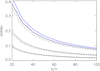 |
Fig. A.1. Dashed black lines – plot of errors (stddev) of CCF positions versus signal-to-noise obtained in 105 simulations of simple spectra consisting of 1, 4 and 16 absorption lines (ordering is top to bottom). Solid black lines – expected trends due to Eq. (A.1) which is larger by approximately 8%. Note that the errors halve for each increase in the number of lines by a factor of 4. Blue lines are the equivalent results for a template A-supergiant spectrum, with the dotted line illustrating the explicit errors obtained from the simulation of Gaussian noise. The dashed blue line has been shifted upwards by 0.02 units for clarity. |
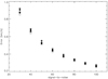 |
Fig. A.2. Cross-correlation error versus signal-to-noise for a simulated BLOeM spectrum: Filled symbols indicate results from the Monte Carlo simulation, open symbols are results derived from Eq. (A.1) modified as discussed in the test. Triangles, circles and stars denote resampled pixel sizes of 14, 7 and 1km s−1 respectively. |
A more realistic second simulation adopted a CMFGEN A-supergiant spectrum with Teff = 9750 K, log g = 2.0 and SMC metallicity as the template spectrum, which has a range of line strengths in the relevant cross-correlation window. This spectrum, as in the above example, is sampled at constant velocity intervals of 1 km s−1 in order compare with the rather simple simulations discussed above. These results are also shown in Fig. A.1, as are the explicit results for the calculated errors assuming Gaussian noise. We see that Eq. (A.1) overestimates the actual errors by about 11% in the case of this template. Similar results are obtained for templates with other representative stellar parameters.
However the situation for the BLOeM data is a little more complicated as the original data are re-binned from the 4000 native wavelength calibrated pixels to a uniform 0.2Å pixel size, or 3056 pixels. For cross-correlation in velocity space these spectra must be resampled to a constant velocity grid of pixels (or logarithmic spacing in wavelength). Typically one might choose a velocity interval that is similar to the original pixel size, in this case ∼14 km s−1, however there may be value in sub-sampling pixels, for example to improve resolution of a final co-added data product. Assuming resampling simply interpolates onto a new wavelength grid, as is the case here, the consideration of Eq. (A.1) tells us that one might expect the errors from this equation need to multiplied by a factor  .
.
This supposition was essentially confirmed with Monte Carlo simulations of cross-correlating an artificial BLOeM spectrum with a range of Poisson noise levels against the original noiseless spectrum. The artificial data were generated from a high resolution CMFGEN spectrum (as above), convolved with FLAMES resolution, and rebinned to 3056 0.2 Å pixels before resampling to a uniform velocity scale. The formal errors from the cross-correlations were calculated as noted above, and the observed errors were determined from 10000 simulations, the formal errors being taken as the mean of the 10000 results individual results. The results are shown in Fig. A.2 confirming that the above procedure for computing the errors in the case of resampling to a smaller pixel size, which is in good agreement with our simulations. We have repeated this Monte Carlo approach for the procedure adopted to measure radial velocities, and outlined in Sect. 3, essentially finding the same result. Namely, the errors inferred from our modified error estimate agree with those derived from our Monte Carlo simulations.
However, since the likely errors due to systematic effects as described in Appendix B likely dominate the error budget for the BAF supergiants we refrain from correcting the formal errors here, and will return to this issue when future data releases are available.
Appendix B: Radial velocity corrections
As was the case for the analysis of the cool, red supergiants from the VFTS survey (Patrick et al. 2019), the FLAMES fields taken on different nights exhibit small temporal drifts in the wavelength calibration, which manifest as an offset in measured radial velocities. This is most noticeable for the AF supergiants that enable high precision measurements due to the number and sharpness of their metal lines. Figure B.1 shows the temporal trends of their radial velocities for each field, from which it is evident that there are correlations between different stars in each field. This is clearly an artifact, most likely due to small thermal drifts affecting the wavelength scale, a known issue for the FLAMES spectrograph.
Velocity corrections (in km s−1) for each field and epoch that have to be added to the measured RVs (available via CDS).
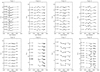 |
Fig. B.1. Measured radial velocities of the A-type supergiants for each BLOeM field (see headings). For ease of comparison, the median value has been subtracted from each source, and multiples of 5 km s−1 added to separate the resulting trends. Note the correlated behaviour across many sources in each field. |
For each field we define a subset of sources that have small dispersion in their mean values, subtract their median velocities, determine the median offset at each epoch across all sources, and correct the observed velocities by this amount. The process is then repeated to convergence, typically only 2–3 iterations per field being required. Table B.1 lists the resulting RV corrections that should be applied to observations in the field at a given epoch, while Fig. B.2 illustrates the impact of their application. Clearly there are still a few issues with some stars. For example, in Field 8, stars 8-010 and 8-091 still display an apparent correlation. However, the full two years of BLOeM data should permit further refinement of this approach.
Measured radial velocities (km s−1) and uncertainties for each epoch (extract).
Mean radial velocities, their standard deviation (σ), median value, and peak-to-peak velocity (p2p). Also listed is the median of individual errors, the number of epochs available, and the number of pairs of measurements satisfying Eq. (1). The effective temperature and logarithmic luminosity are those derived here and used in construction of the HRD. Candidate spectroscopic binaries are flagged as ‘var’ according to Fig. 4 and ‘LP’ marks the potential long period system that does not meet the binary threshold. Candidate α Cyg variables are also indicated. The full version of this table is available via the CDS.
Appendix C: Radial velocity plots of candidates variables
In this appendix we plot the epoch RV data of all 14 sources satisfying Eqs. 2 and 1, Figs. C.1 and C.2, plus three examples of sources that do not pass the variability criteria yet exhibit signs of long-term correlated variability, Fig. C.3, that may indicate binarity or potentially (long-term) pulsations.
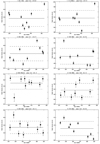 |
Fig. C.1. Radial velocity plots as function MJD for sources flagged as var in Table B.3. Headers give the BLOeM identifiers, spectra types, peak-to-peak velocities, and number of velocity pairs satisfying Eq. (1). The horizontal solid lines indicate the mean velocities, and the dashed lines the standard deviations. |
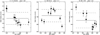 |
Fig. C.3. Radial velocity plots as a function MJD for sources exhibiting possible binary motion, or perhaps long-term pulsation. Headers list the BLOeM identifiers, spectra types, and peak-to-peak velocities 1. The horizontal solid lines indicate the mean velocities, and the dashed lines the standard deviations. |
All Tables
Number of targets and median peak-to-peak RV measurements (Δvmed) as a function of spectral sub-type for the BAF supergiants.
Range of orbital parameters and their assumed distributions considered in the bias correction calculations.
Velocity corrections (in km s−1) for each field and epoch that have to be added to the measured RVs (available via CDS).
Measured radial velocities (km s−1) and uncertainties for each epoch (extract).
Mean radial velocities, their standard deviation (σ), median value, and peak-to-peak velocity (p2p). Also listed is the median of individual errors, the number of epochs available, and the number of pairs of measurements satisfying Eq. (1). The effective temperature and logarithmic luminosity are those derived here and used in construction of the HRD. Candidate spectroscopic binaries are flagged as ‘var’ according to Fig. 4 and ‘LP’ marks the potential long period system that does not meet the binary threshold. Candidate α Cyg variables are also indicated. The full version of this table is available via the CDS.
All Figures
|
Fig. 1. Hertzprung–Russell diagram (HRD) of the BLOeM survey highlighting the BAF supergiant sample studied in this article with large star symbols colour-coded based on spectral type, as indicated by the legend. The three targets with the black circles indicate the only targets in this sample that have a clear indication of binarity: BLOeM 4-072, BLOeM 6-006, and BLOeM 6-008. The three targets with the black squares indicate targets that display a binary motion characteristic of long orbital periods: BLOeM 1-114, BLOeM 3-106, and BLOeM 8-001. Stellar parameters are determined using a calibration to spectral types by Paper I. Grey points show the entire BLOeM sample and stellar tracks from the extended grid of Schootemeijer et al. (2019) with mass-dependent overshooting (described in Appendix B of Hastings et al. 2021). The black marker with error bars on the left gives an indication of the typical uncertainties on the stellar parameters. The solid red line shows the magnitude limit imposed by the BLOeM survey target selection. The dashed red line is the Humphreys–Davidson (HD) limit, the cool part of which is shown as the revised-down limit in the SMC from Davies et al. (2018). |
| In the text | |
|
Fig. 2. Spatial location of the BAF-type supergiant sample in the SMC, overlaid on the density map of the Gaia DR3 source catalogue (G < 19 mag). Spectral types of the targets are colour-coded as indicated. Black circles mark the locations of the eight BLOeM fields. |
| In the text | |
|
Fig. 3. A montage of BAF supergiant star spectra from BLOeM (in black) and best matching theoretical template spectra (blue) from CMFGEN/ATLAS model grids (see text). BLOeM IDs and spectral types are noted above each spectrum. Template spectra were used to determine an absolute RV scale, and one can see good agreement between line positions and strengths of the templates with the data. The vertical dashed lines indicate the spectral region that was used to derive the cross-correlation functions (CCFs) for all sources. We highlight the slight mismatch of the continuum for the F supergiant, BLOeM 1-102. For cool stars, the automatic continuum placement is more difficult due to the line density of the spectra; however, the CCFs are not impacted by this offset as we use normalised CCFs, such that the mean signal is subtracted from each spectrum before cross-correlation. We note that the A–F supergiant line spectra are dominated by Fe II and Fe I lines (for line lists, see Venn 1995, 1999). |
| In the text | |
|
Fig. 4. Histogram of peak-to-peak radial-velocity (RV) measurements (Δv) for the BAF supergiant sample. Different colours highlight the sub-samples as indicated in the panel. The dashed black line is the chosen threshold for binarity in the multiplicity analysis. |
| In the text | |
|
Fig. 5. Left panel: Peak-to-peak RV (Δv) as a function of stellar radius for the BAF supergiants and the B3 supergiants of Britavskiy et al. (2025). Radii were determined using effective temperatures and luminosities from Table B.3. The sizes of the symbols in both panels are determined by Δv/σΔv. Black circles mark stars of the cohort of variable late-B-type bright giants. Right panel: HRD for BAF supergiant sample using stellar parameters listed in Table B.3; symbols have the same meaning as in the left panel. We note that the sources with largest Δv/σΔv tend to be the most luminous and hottest stars. |
| In the text | |
|
Fig. 6. Radial-velocity (RV) time series for four of the targets that display RV variability above the chosen thresholds (see text), with spectral types of A Ia (BLOeM 1-051), B9 Ia (1-112), B8 Ia (2-093), and A2 Ia (6-008). Identifications are listed in the panel headings, as are the mean RVs and their standard deviations, which are indicated in each panel by solid and dashed lines, respectively. We note that only 6-008 displays evidence of a long-term RV trend that might be a signature of binary motion. Due to their large radii, all of these stars have minimum periods of ∼100 days or more. |
| In the text | |
|
Fig. 7. Left: Orbital period shown against mass ratio (q) for simulated binary systems in the orbital period ranges that were used to correct for our observational biases. Solid black contour lines show the probability of detection at the 99, 90, 50, and 10% levels given the temporal baseline and typical uncertainties of the BLOeM data, where each grid point is the median of 10 000 simulated systems. The detection criteria used in these simulations are matched to those of the observations (i.e. Δv = 5 km s−1 and σ = 4). The dashed coloured lines show the minimum allowed orbital period for three representative examples as a function of the mass ratio of the system. Right: Same simulations where the solid contour lines now show lines of constant semi-amplitude velocity on the 150, 100, 50, 25, and 10 km s−1 levels. |
| In the text | |
|
Fig. 8. Colour-magnitude diagram using 754 BLOeM sources found in the UVIT FUV catalogue (Hota et al. 2024), colour-coded by spectral type. The FUV magnitude was obtained with the F172M filter, while the BP − RP colour is from GaiaBp and Rp filters. The five outliers described in Sect. 4.4 are flagged with black circles. |
| In the text | |
|
Fig. 9. Fraction of detected binarity as function of Δvlim. The solid black line in the left panel shows the B5–9 supergiants, and the right panel is the same, except for AF supergiants. The dashed red lines show the simulated binary fraction assuming an intrinsic binary fraction on the main sequence of 75 ± 10% – to roughly match that of Villaseñor et al. (2025) – which was evolved to remove binary systems that would have since interacted based on the current sizes of the stars. The solid red lines show the bounds of the assumed uncertainty on the intrinsic multiplicity fraction. |
| In the text | |
|
Fig. A.1. Dashed black lines – plot of errors (stddev) of CCF positions versus signal-to-noise obtained in 105 simulations of simple spectra consisting of 1, 4 and 16 absorption lines (ordering is top to bottom). Solid black lines – expected trends due to Eq. (A.1) which is larger by approximately 8%. Note that the errors halve for each increase in the number of lines by a factor of 4. Blue lines are the equivalent results for a template A-supergiant spectrum, with the dotted line illustrating the explicit errors obtained from the simulation of Gaussian noise. The dashed blue line has been shifted upwards by 0.02 units for clarity. |
| In the text | |
|
Fig. A.2. Cross-correlation error versus signal-to-noise for a simulated BLOeM spectrum: Filled symbols indicate results from the Monte Carlo simulation, open symbols are results derived from Eq. (A.1) modified as discussed in the test. Triangles, circles and stars denote resampled pixel sizes of 14, 7 and 1km s−1 respectively. |
| In the text | |
|
Fig. B.1. Measured radial velocities of the A-type supergiants for each BLOeM field (see headings). For ease of comparison, the median value has been subtracted from each source, and multiples of 5 km s−1 added to separate the resulting trends. Note the correlated behaviour across many sources in each field. |
| In the text | |
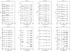 |
Fig. B.2. Same as Fig. B.1 but with the corrections as tabulated in Table B.1. |
| In the text | |
|
Fig. C.1. Radial velocity plots as function MJD for sources flagged as var in Table B.3. Headers give the BLOeM identifiers, spectra types, peak-to-peak velocities, and number of velocity pairs satisfying Eq. (1). The horizontal solid lines indicate the mean velocities, and the dashed lines the standard deviations. |
| In the text | |
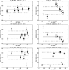 |
Fig. C.2. Same as Fig. C.1 but for other sources. |
| In the text | |
|
Fig. C.3. Radial velocity plots as a function MJD for sources exhibiting possible binary motion, or perhaps long-term pulsation. Headers list the BLOeM identifiers, spectra types, and peak-to-peak velocities 1. The horizontal solid lines indicate the mean velocities, and the dashed lines the standard deviations. |
| In the text | |
Current usage metrics show cumulative count of Article Views (full-text article views including HTML views, PDF and ePub downloads, according to the available data) and Abstracts Views on Vision4Press platform.
Data correspond to usage on the plateform after 2015. The current usage metrics is available 48-96 hours after online publication and is updated daily on week days.
Initial download of the metrics may take a while.