| Issue |
A&A
Volume 698, June 2025
|
|
|---|---|---|
| Article Number | A201 | |
| Number of page(s) | 14 | |
| Section | Cosmology (including clusters of galaxies) | |
| DOI | https://doi.org/10.1051/0004-6361/202452649 | |
| Published online | 17 June 2025 | |
Inference of the morphology and dynamical state of nearby Planck-SZ galaxy clusters with Zernike polynomials
1
Dipartimento di Fisica, Sapienza Università di Roma, Piazzale Aldo Moro 5, I-00185 Roma, Italy
2
Physics Department “Ettore Pancini”, Università degli studi di Napoli “Federico II”, Via Cintia 21, I-80126 Napoli, Italy
3
Institute for Astronomy, University of Edinburgh, Royal Observatory, Edinburgh EH9 3HJ, UK
4
Departamento de Física Teórica, Módulo 8, Facultad de Ciencias, Universidad Autónoma de Madrid, E-28049 Madrid, Spain
5
Centro de Investigación Avanzada en Física Fundamental (CIAFF), Facultad de Ciencias, Universidad Autónoma de Madrid, E-28049 Madrid, Spain
6
University of Lyon, UCB Lyon 1, CNRS/IN2P3, IP2I Lyon, France
⋆ Corresponding author: This email address is being protected from spambots. You need JavaScript enabled to view it.
Received:
17
October
2024
Accepted:
7
April
2025
Abstract
Aims. We analyse maps of the Sunyaev–Zel’dovich (SZ) signal of local galaxy clusters (z<0.1) observed by the Planck satellite to classify their dynamical state via morphological features.
Methods. We applied a novel method, which was recently employed on mock SZ images generated from hydrodynamical simulated galaxy clusters in THE THREE HUNDRED (THE300) project to study the morphology of the cluster maps. In this paper, we report our results following its first application on real data. The method consists of modelling the images with a set of orthogonal functions defined on circular apertures, namely, the Zernike polynomials. From the fit we computed a single parameter, 𝒞, that quantifies the morphological features present in each image. The link between the morphology of 2D images and the dynamical state of the galaxy clusters is well known, even if it is not obvious. We used mock Planck-like Compton parameter maps generated for THE300 clusters to validate our morphological analysis. These clusters are, in fact, properly classified for their dynamical state with the relaxation parameter, χ, by exploiting 3D information from the simulations.
Results. We find a mild linear correlation of ∼38% between 𝒞 and χ for THE300 clusters, mainly affected by the noise present in the maps. To obtain a proper dynamical-state classification for the Planck clusters, we exploited the conversion from the 𝒞 parameter derived in each Planck map in χ. A fraction of the order of 63% of relaxed clusters has been estimated in the selected Planck sample. Our classification was then compared with those of previous works that have attempted to evaluate, with different indicators and/or other wavelengths, the dynamical state of the same Planck objects. We find an agreement with these other works to be greater than 58%.
Key words: methods: numerical / methods: observational / methods: statistical / galaxies: clusters: general / galaxies: clusters: intracluster medium
© The Authors 2025
 Open Access article, published by EDP Sciences, under the terms of the Creative Commons Attribution License (https://creativecommons.org/licenses/by/4.0), which permits unrestricted use, distribution, and reproduction in any medium, provided the original work is properly cited.
This article is published in open access under the Subscribe to Open model. This email address is being protected from spambots. You need JavaScript enabled to view it. to support open access publication.
1. Introduction
Galaxy clusters constitute the final stage of the hierarchical structure formation process (see e.g. Voit 2005) and their census in terms of mass and redshift distribution is one of the ways we can place constraints on cosmological parameters (see e.g. Planck Collaboration XX 2014; Planck Collaboration XXIV 2016; Planck Collaboration VI 2020). The accurate estimation of the mass is certainly the main ingredient in setting cosmological constraints from galaxy cluster abundances. Different approaches have been explored to infer the mass, given it is not a direct observable and, thus, these have been based on simplified assumptions. For example, assuming a self-similar model (Kaiser 1986), several scaling relations have been defined to relate the mass to multi-wavelengths observables and are used to constrain the mass when dealing with large samples of systems (see e.g. Giodini et al. 2013; Pratt et al. 2019). However, some simplified hypotheses have been used, such as the hydrostatic equilibrium based on spherical distribution for dark matter and baryon content (see e.g. Kravtsov & Borgani 2012). It is well known that during their evolution, galaxy clusters can experience states of non-equilibrium, for example, during merger events. This condition may introduce biases in mass computation (Planck Collaboration XX 2014). Classifying clusters according to their dynamical state can help account uncertainties in these methods. From an observational point of view, the analysis of the morphological appearance of cluster images generated at different wavelengths is the cheapest way to attempt a dynamical-state assessment. The presence of irregularities at different scales in the images can in fact be sign of dynamical activities in the systems not related to the conditions of equilibrium described before. The first approach to the morphological analysis was carried out through visual classifications of cluster images from X-ray observations (Jones et al. 1992). However, this is a method that is subjective and challenging when applied to large samples. Different techniques were then developed to speed up and make these analyses more robust; for instance, defining several parameters that can quantify morphological differences between images. Some of the most commonly used are, for example, the centroid shift (Mohr et al. 1993; O’Hara et al. 2006), the power ratios (Buote & Tsai 1995), the asymmetry (Schade et al. 1995), the cuspiness of the gas density profile (Vikhlinin et al. 2007), the concentration ratio (Santos et al. 2008), the central gas density (Hudson et al. 2010), and the Gini coefficient (Parekh et al. 2015). They are used singularly or combined together (see e.g. Rasia et al. 2013; Mantz et al. 2015; Lovisari et al. 2017; Cialone et al. 2018; Bartalucci et al. 2019; De Luca et al. 2021; Campitiello et al. 2022), taking into account the cluster apertures to analyse; for example, being sensitive to the cores or to characteristic radii (e.g. R5001, R200, and so on). Several approaches are employed considering the different cluster components, namely, galaxies and gas (see e.g. Ribeiro et al. 2013; Wen & Han 2013; Lopes et al. 2018; Cerini et al. 2023). For example, by using optical and X-ray data, it is possible to measure the offset between the position of the bright central galaxy (BCG) and the X-ray peak or centroid (see e.g. Jones & Forman 1984; Lavoie et al. 2016; Lopes et al. 2018; De Luca et al. 2021) or the other bright member galaxies (Casas et al. 2024). Also, the magnitude difference between the first and second BCGs can be employed as a dynamical state indicator, as shown in Lopes et al. (2018). To date, a large literature is available about the definition and the application of morphological parameters both on X-ray and optical observations. Several works also applied these methods on simulated data (see e.g. Cao et al. 2021; De Luca et al. 2021; Li et al. 2022; Seppi et al. 2023). Recently, the morphological analysis of galaxy clusters has been also extended to simulations of millimetre observations through the Sunyaev-Zel’dovich (SZ) effect (Cialone et al. 2018; De Luca et al. 2021; Capalbo et al. 2021, C21 hereafter). The SZ effect, in fact, has opened a new window to produce large samples of galaxy clusters. It is a spectral distortion of the cosmic microwave background (CMB) radiation caused by the interaction, via inverse Compton scattering, of the photons with the energetic free electrons in the intracluster medium (ICM) (Sunyaev & Zeldovich 1972). In particular, the thermal component of the SZ effect (tSZ), which depends on the thermal random motion of the electrons, causes a boost in the energy of the CMB photons resulting in an increase of the CMB brightness at frequencies ≳217 GHz in the direction of the clusters (see e.g Mroczkowski et al. 2019, for a review). The intensity of the effect is quantified with the Compton parameter, y:
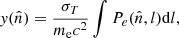 (1)
(1)
where σT is the Thomson scattering cross-section, me is the electron rest mass, c is the speed of light, Pe is the electron pressure and the integration is done along the line of sight, l, in the direction,  . The advantages of tSZ surveys with respect to X-ray ones are two-fold: the independence of the spectral distortion from the redshift and the linear dependence of y from the electron pressure (at least in the non-relativistic approximation). These features make the tSZ effect well suited to observe the most distant clusters and construct samples that are, in principle, mass-limited and representative of the underlying population. Several instruments have been devoted to observe galaxy clusters through the tSZ effect. The Planck satellite made it possible to produce full-sky Compton parameter maps (i.e. y-maps) (Planck Collaboration XXII 2016) and a catalogue of tSZ sources, which, in its last release from the full-mission data (Planck Collaboration XXVII 2016), contains 1653 detections with 1203 confirmed clusters from ancillary data. The South Pole Telescope (SPT) was the first ground-based instrument suitable to observe distant galaxy clusters through the tSZ effect (Staniszewski et al. 2009). Since then, a large number of clusters have been detected in several SPT surveys (Bleem et al. 2015, 2020; Huang et al. 2020), with also the recent release of a y-map covering ∼2500 deg2 of the southern sky at 1.25′ resolution Bleem et al. (2022). The redshift coverage of tSZ-selected galaxy clusters has been improved with the Atacama Cosmology Telescope (ACT) that, as in the case of SPT, provided several samples of clusters during the years (Hilton et al. 2018, 2021). The last catalogue derived from this survey (Hilton et al. 2021) contains >4000 optically confirmed clusters, with 222 at z>1 and a total of 868 systems that are new discoveries, while a new y-map at 1.6′ resolution and covering ∼13 000 deg2 of the sky has been recently released (Coulton et al. 2024).
In this work, we use the all-sky y-map provided by the Planck satellite to study the morphology of nearby (z<0.1) galaxy clusters. We have applied the method developed in C21, which consists in modelling the maps analytically by using the Zernike polynomials (ZPs, hereafter) to quantify their different morphologies. This approach was tested in C21 on a set of high-resolution y-maps generated from synthetic clusters in THE THREE HUNDRED project2 (hereafter THE300; Cui et al. 2018). Modelling with the ZPs has proven to be a suitable way to analyse a wide variety of images, providing a chance to explore different spatial scales in the maps simply by changing the number of ZPs used and to reveal the main features for a good morphological classification. In C21, a single parameter, 𝒞, was introduced to collect the capability of ZPs to describe the different morphologies in the y-maps. 𝒞 showed a good correlation with most common morphological parameters used in the literature and also with a combination of some proper dynamical state indicators available, in that case, from simulations (De Luca et al. 2021). Motivated by those results, here we apply the Zernike modelling for the first time on real data. The aim of this work is to deduce a morphological classification for the Planck-SZ clusters, using the y-maps and to verify if this analysis can allow for their dynamical state to be inferred. To this end, we compiled a set of mock Planck-like y-maps realised from THE300 clusters for which the dynamical state could be estimated a priori from 3D data. We then tested whether and how our morphological analysis of y-maps can be related to a proper dynamical classification of the clusters in the Planck sample. The link between the morphology and the dynamical state is, in fact, not obvious. Some limitations due, for instance, to projection effects or limited angular resolutions in the maps can reduce the capability to reveal characteristic features indicative of the dynamical state.
The study of the dynamical state of samples of Planck clusters was already conducted in several works (Rossetti et al. 2016, 2017; Lovisari et al. 2017; Andrade-Santos et al. 2017; Lopes et al. 2018; Campitiello et al. 2022) by using X-ray or optical observations. In this work, we would like to provide a more complete view on this question by exploiting also the available millimetre data. Finally, we compare our classification with the ones reported in literature.
The paper is structured as follows. In Section 2, we introduce the data sets. In Section 3, we recall the ZPs definition and the method employed to model the y-maps. In Section 4, we report the results of the application of ZPs as morphological indicators and the calibration to infer the dynamical state. In Section 5, we analyse a comparison with the literature data and our conclusions are summarised in Section 6. Throughout this work, we assume a ΛCDM cosmology with H0 = 67.8 km s−1 Mpc−1, Ωm = 0.307, and ΩΛ = 0.048 (Planck Collaboration XIII 2016).
2. Datasets
2.1. The Planck-SZ clusters sample and y-maps
We selected a sample of galaxy clusters from the second Planck catalogue of Sunyaev–Zel’dovich sources (PSZ2, Planck Collaboration XXVII 2016). Specifically, we used one of the two sub-samples extracted from the PSZ2 for cosmology studies (Planck Collaboration XXIV 2016; Planck Collaboration VI 2020), namely, the intersection catalogue (PSZ2_cosmo, hereafter). This catalogue was constructed by considering the detections made by all the three different algorithms used for the PSZ2, namely, two matched multi-filters techniques, MMF1 and MMF3 (Melin et al. 2006, 2012), and the PowellSnakes (PwS) method (Carvalho et al. 2009, 2012). All clusters show a signal-to-noise ratio (S/N)>6. The catalogue covers 65% of the sky, excluding the Galactic plane and bright point sources that can lead to spurious detections. We excluded clusters with potential infrared contamination, indicated in the catalogue with a proper flag ([IR_FLAG] = 1). We also excluded the clusters without redshift association. As the second step in defining the sample, we used the mass estimate, M500, provided in the catalogue, to compute the angular radius θ500 of the clusters. Planck Collaboration XXVII (2016) specified that the mass value is derived using the scaling relation Y500−M500 from Planck Collaboration XX (2014), in which a mean bias of (1−b) = 0.8 is assumed between the true mass and the hydrostatic mass. Therefore, we corrected the mass values in the catalogue for the bias above to obtain an estimate of the true mass of the clusters. The simulated cluster masses are selected to be consistent with them, as described in Section 2.2. From  , where ρc(z) is the critical density of the Universe at redshift z, we compute the cluster radius R500; hence, the respective angular size of θ500=R500/DA(z), where DA(z) is the angular diameter distance. Since the y-maps that we use have a resolution of 10′, as described in the next section, we selected only the resolved objects at z<0.1, namely, the clusters with θ500⩾10′. Our final sample is composed by 109 clusters. In Fig. 1 we show the distribution of the clusters in the M500−z plane in red.
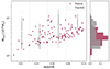 |
Fig. 1. Distribution in the M500−z plane of 109 Planck-SZ clusters (red triangles) selected for the morphological analysis (see Section 2.1). The thin dashed vertical lines mark the redshift bins used for the comparison with the synthetic clusters (grey dots) from THE300 project (see Section 2.2). In the right panel, we give the normalised distributions of the masses for the Planck (in red) and THE300 (in grey) samples. |
The publicly available all-sky y-maps, described in Planck Collaboration XXII (2016), were constructed by combining the Planck single-channel maps convolved to a common resolution of 10′ and using two different component separation algorithms: Modified Internal Linear Combination Algorithm (MILCA, Hurier et al. 2013) and Needlet Independent Linear Combination (NILC, Remazeilles et al. 2011). In this work, we limited the analysis to the MILCA y-map. The all-sky y-maps have been released in HEALPIX3 format (Gorski et al. 2005), with Nside = 2048 and pixel size of 1.7′. We used HEALPY (Zonca et al. 2019), a specific Python package to process HEALPIX maps, to extract the y-maps of each cluster. These latter are square cut-outs of side-length equal to 2θ500, drawn as gnomonic projections from the all-sky y-map and with the same pixel resolution of the HEALPIX map. Each cut-out is centred on the cluster coordinates reported in the PSZ2 catalogue. On these maps we overlap a circular aperture of radius θ500 to define the domain the Zernike modelling should be applied to. We also normalised the signal distribution to the maximum value of y within the aperture.
2.2. THE THREE HUNDRED project
THE300 project (Cui et al. 2018) is a large catalogue of hydrodynamically simulated galaxy clusters. The basis of the sample is composed by 324 large spherical regions, with radius of 15 h−1 Mpc, selected within the DM-only MultiDark simulation (MDPL2, Klypin et al. 2016). These are the regions with most massive objects (virial mass ≳8×10¹⁴ h−1 M⊙ at z = 0) at their centre, which have been re-simulated with different baryonic physics models. We used the catalogue of galaxy clusters generated with the smoothed-particle hydrodynamics (SPH) code GADGET-X (Beck et al. 2016), which includes black hole and active galactic nuclei feedback. Overall, 128 redshift snapshots, from z = 0 to z = 17, were generated for each re-simulated region and the halo finder AHF (Knollmann & Knebe 2009) was used to identify the virialised structures. Here, we selected four redshift snapshots, at z = 0.022,0.044,0.068, and 0.092, to cover the redshift range of the PSZ2_cosmo sample. The mass distribution along the different redshifts is plotted in Fig. 1 in grey.
2.2.1. Mock Planck-like y-maps
For THE300 galaxy clusters, mock y-maps are generated by using the PYMSZ code4, as described in Cui et al. (2018). The procedure consists of discretising Eq. (1), as follows:
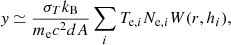 (2)
(2)
where dA is the projected area orthogonal to the line of sight, dl. Then, Te,i and Ne,i are the temperature and the number of electrons of the ith gas particle, respectively, W(r,hi) is the SPH kernel adopted in the hydrodynamical simulations to smear out the y signal from each gas particle and hi is the gas smoothing length. For the morphological analysis we performed in this work, it is necessary to compare mock y-maps that are representative, in terms of features in the maps and then of S/N, of the real Planck y-maps. Therefore, the mock maps are convolved with a Gaussian kernel with 10′ FWHM and gridded in pixels of 1.7′ in size to mimic the angular resolution of the real maps. Then, the Planck instrumental noise is also taken into account, following a procedure similar to the one described in Ruppin et al. (2019). A full-sky noise map can be produced by using the Planck noise power spectrum and the full-sky map of the standard deviation of the Compton parameter (Planck Collaboration XXII 2016). From this noise map, cut-outs are extracted randomly, considering the position of the galaxy clusters in the PSZ2 catalogue and then added to the mock y-maps to generate Planck-like y-maps. We note that point source contamination is not included in these mock y-maps. Additional details of the realisation of the Planck-like maps are reported in de Andres et al. (2022), in which these maps are used to infer galaxy clusters masses with a deep learning approach. Finally, in each of the four redshift snapshots selected above, we extracted the Planck-like maps with S/N ∈ [min(S/N)Planck, max(S/N)Planck]. Thus, the number of THE300 clusters selected in each bin are, respectively, 283, 209, 434, and 295 (see the grey dots in Fig. 1). As for the real Planck y-maps, we used a circular aperture of radius θ500 to define the region to be modelled.
2.2.2. Dynamical state of THE300 clusters
Being a set of synthetic clusters, for THE300, we can define the dynamical state by taking into account the 3D information from the simulations (Cui et al. 2017, 2018; Haggar et al. 2020; Zhang et al. 2022). In particular, a single parameter, χ, which combines different indicators of the dynamical state, has been defined and it is already in use to segregate different populations in galaxy clusters samples (see e.g. C21, Haggar et al. 2020; De Luca et al. 2021). This study is focussed on R500 apertures therefore we refer to the definition of χ in De Luca et al. (2021), also used in C21, where only two indicators are adopted in the following way:
 (3)
(3)
where
 (4)
(4)
is the total sub-halo mass fraction. Here, M500 is the mass of the cluster computed in a volume of radius equal to R500 and Mi are all the sub-halo masses in the same volume. Furthermore,
 (5)
(5)
is the centre-of-mass offset, where rcm is the centre-of-mass position of the cluster and rc is the centre of the cluster identified with the highest density peak. Following the suggestions in De Luca et al. (2021), relaxed and disturbed systems can be identified, respectively, with log10χ>0 and log10χ<0.
3. Methods
To study the morphology of the y-maps of the clusters, we employed the method developed in C21. This method involves modelling the maps using ZPs and deriving a single parameter from the fitting process to quantify the differences between the maps. We detail this procedure below, after describing the main properties of ZPs.
3.1. Zernike polynomials
The ZPs (Zernike 1934) are a complete basis of orthogonal functions defined on a unit disc. They are widely used to describe aberrations in optical systems (see e.g. Mahajan et al. 2007) and a common application is in adaptive optics. They are also used to model aberrated wavefronts from atmospheric turbulence (see e.g. Noll 1976; Rigaut et al. 1991). More generally, orthogonality and completeness make these polynomials very useful to fit and analyse functions on circular domains. Indeed, they are also applied in a variety of research fields as pattern descriptors (see e.g. Niu & Tian 2022, for a review). We refer to the analytical definition of ZPs given in Noll (1976):
 (6)
(6)
where n is the polynomial order ( , n⩾0), m is the azimuthal frequency (
 , m⩽n, n−m= even), ρ and θ are the polar coordinates (0⩽ρ⩽1, 0⩽θ⩽2π),
  is a normalisation factor and
 (7)
(7)
is the radial function. The orthogonality property is given by
 (8)
(8)
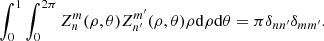
The y parameter in cluster maps can be modelled as a weighted sum of ZPs as in the following:
 (9)
(9)
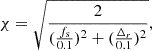
where cn,±m are the expansion coefficients that quantify the weight of each polynomial in the fit, while the maximum polynomial order, n, used in the expansion is chosen according to the desired accuracy for modelling the map. In this regard, we emphasise that the goal of this work is to recognise the morphological regularity of the maps – or rather, to verify if there are inhomogeneities in the distribution of the signal (e.g. clumpy or multi-peaks distributions). This does not require a modelling of the maps in all their details, as already noted in C21. In addition, to finalise the modelling we have to take into account the characteristics of our sample in terms of angular resolution in the maps and of the residual noise contamination. We refer to the study in Svechnikov et al. (2015) and the discussion in Appendix A in C21 to select a suitable number of ZPs for our analysis. The resolving capability of a Zernike expansion of order n, in terms of spatial frequencies, k, and in units of the inverse radius of the circular aperture, can be roughly derived from k≈(n+1)/2π, as described in Svechnikov et al. (2015). We emphasise that this is a simple criterion to obtain an estimate of the spatial resolution that can be reached by using a set of ZPs. However (as shown in Appendix A in C21, considering the power spectra of the y-maps and of the respective Zernike fitting maps), the agreement between modelling and data, for the morphological analysis we are interested in, is still reasonable beyond the value of k derived from the approximation above. In particular, by using a maximum polynomial order of n = 8 the spatial resolution estimated in C21 was ∼0.5θ500. In Svechnikov et al. (2015), an empirical criterion was derived to also estimate the spatial resolution of a Zernike modelling obtained when changing the maximum order, n, of the expansion: an increase (decrease) of n of a certain factor corresponds to an increase (decrease) of the spatial resolution of the same factor. The Planck y-maps that we analyse here have a low angular resolution (10′, see Section 2.1) and the internal regions of radius <θ500 are poorly resolved; therefore, we want to limit the modelling on the scale of the map dimension, namely, 2θ500. We need a spatial resolution that is about four times lower with respect to the resolution estimated in C21 and we have to reduce the maximum order n of the expansion of the same factor. Thus, we modelled the Planck y-maps with only six ZPs, up to the order of n = 2. We describe in Section 4.2 how this choice also allows us to be poor sensitive to the residual noise in the maps.
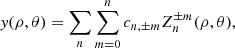
3.2. The morphological parameter 𝒞
From the Zernike fit we derive a parameter, 𝒞, given by
 (10)
(10)
where cn,±m are the Zernike expansion coefficients defined in Eq. (9) and the sum, as explained before, is truncated to n = 2. The coefficients cn,±m are derived from Eq. (9) by exploiting the orthogonality of the polynomials as expressed in Eq. (8). They are normalised to the area of the circular aperture and, thus, computed from
 (11)
(11)
where R500,px is the radius expressed in pixels and the sum is extended to all the pixels. The fit procedure is implemented using the Python package POPPY5 (Perrin et al. 2012) for calculating ZPs. By moving from the minimum to the maximum value of 𝒞 the maps are recognised as increasingly irregular. We note that in the definition in Eq. (10), the coefficients related to ZPs with m = 0 are neglected. Indeed, in C21, it was shown that the overall contribution of those polynomials is almost invariant when modelling different maps in a wide range of morphologies, then they are not able to distinguish morphological details needed for an accurate classification. On the contrary, the weight of ZPs with m≠0 is negligible when modelling regular (mostly circular) distributions in the maps and it increases in case of complex patterns involving, for example, asymmetries or sub-structures (see Fig. 2). This behaviour is further explained with some examples in the next section.
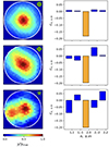 |
Fig. 2. Left: Examples of Planck y-maps of three clusters with different values of the 𝒞 parameter. Top: cluster PSZ2 G075.71+13.51 (PSZ2 index 322). Middle: cluster PSZ2 G340.88−33.36 (PSZ2 index 1591). Bottom: cluster PSZ2 G093.94−38.82 (PSZ2 index 430). Each map is centred on the cluster position reported in the PSZ2 catalogue, with side-length equal to 2θ500. The white circle is the aperture defined for the Zernike fit. The markers in green in the top-right corner of each map are used to indicate the respective values of the 𝒞 parameter in Fig. 3. Right: Bar charts of the cn,±m coefficients (see Eq. (11)) resulting from the Zernike fit applied on each map on the left. The ZPs on the x axis are ordered following the Noll's scheme (Noll 1976). The polynomial order n increases from left to right. Orange and blue bars refer to ZPs with m = 0 and m≠0, respectively. |
4. Results
In this section we report the results of the Zernike fit applied both on the Planck y-maps and on the mock Planck-like y-maps. Then, we describe how to convert the morphological analysis derived from the fit in a dynamical-state evaluation.
4.1. Analysis of the Planck sample
We applied the Zernike fit on the y-maps of the PSZ2_cosmo sample described in Section 2.1. We show in Fig. 2 three examples of Planck y-maps with the results of the respective Zernike fits. In the left panels, there are the y-maps centred on the clusters coordinates, with the solid white line defining the circular aperture of radius equal to θ500 for each cluster. On the right side of the figure, there are the bar charts of the coefficients cn,±m of each ZP used to fit the maps. The ZPs are ordered as in Noll (1976) (see also Fig. 1 in C21), with the order n increasing when moving from left to right, and they are grouped for the azimuthal frequency (m = 0 in orange and m≠0 in blue). We note that the coefficient c00 related to the first polynomial (i.e.  ) is neglected because it is just equal to the mean value of y inside the circular aperture. In the top-left panel there is an example of map with a clear circular symmetry: the contribution of ZPs with m≠0 is minimal. The map in the middle-left panel shows an overall prolate distribution but with no resolved sub-structures and in the fit the weight of ZPs with m≠0 is larger. Instead, in the third map (bottom-left) there is evidence of a possible sub-structure with respect to the central target and all the ZPs with m≠0 have a non-negligible value. As already described, we stress that the coefficients of ZPs with m = 0 have small differences between the fits. In Fig. 3, we show the cumulative distribution of the number of clusters along 𝒞 for the full sample of clusters. The median value of the distribution is 𝒞 = 0.58, while the 16th and 84th percentiles are at 𝒞 = 0.43 and 0.76, respectively. For convenience, in Fig. 3, we also indicate the value of the 𝒞 parameter for the three maps shown in Fig. 2, using the following markers: a circle for the most regular map (top) that has 𝒞 = 0.35, a diamond for the intermediate case (middle) with 𝒞 = 0.63, and a star for the irregular map (bottom) with 𝒞 = 0.99. The values of 𝒞 for each cluster in PSZ2_cosmo are reported in Table A.1..
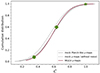 |
Fig. 3. Cumulative distribution of the number of clusters along the 𝒞 parameter. The red line refers to the PSZ2_cosmo sample, the grey lines refer to the sample selected from THE300, and considering, respectively, their Planck-like maps (solid line) and their maps without noise (dashed line). The green markers are used to indicate the value of 𝒞 for the three maps shown in Fig. 2. |
It is well known that the study of the morphology of cluster maps, even if a useful method to attempt a cluster dynamical classification, has some limits. In fact, projection effects, limited angular resolution observations, and noise contamination in the maps can affect the conclusions on the real state of the clusters. Therefore, it is also important to quantify the efficiency of the morphological analysis in inferring information on the dynamical state. To do so, here we use the synthetic data set described in Section 2.2, by exploiting the a priori knowledge of the dynamical state derived from the simulations.
4.2. Analysis of THE300 sample
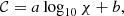
In Section 2.2, we describe the sample of clusters selected from THE300 to reproduce the PSZ2_cosmo (see Fig. 1). We modelled their Planck-like y-maps with the ZPs in the same way as we did for the real Plank y-maps. In Fig. 3, we show the cumulative distribution of THE300 clusters along 𝒞 with the solid line in grey and we compare it with the cumulative of the PSZ2_cosmo. It is evident that the two distributions are compatible. We confirm this with a two-sample Kolmogorov–Smirnov (KS) test. The KS test is a non-parametric method to quantify the differences between the cumulative distributions of two samples. It provides the KS statistic, which is a measure of the maximum deviation between the two cumulatives, and the p-value of the null hypothesis that the two distributions are identical. In our case, KS statistic = 7.1×10⁻² and p-value = 0.67. Thus, we cannot reject the null hypothesis and this means that the mock y-maps are sufficiently representative of the Planck y-maps, that is, they display the same morphology. This allows us to pose some questions regarding whether this morphological classification is representative of the dynamical state of the clusters and/or whether the morphology deduced from y-maps is correlated to the dynamical state defined from 3D information. To answer to these questions, we studied the correlation between the 𝒞 parameter and the χ indicator (we consider its log10) for THE300. We performed 104 resamplings of the data set with a bootstrap method and we estimated the mean Pearson correlation coefficient 〈r〉=−0.38±0.03. In Fig. 4 (in blue), we show 𝒞 along log10χ, binning in log10χ. The triangles are the mean value of 𝒞 in each bin of log10χ and the shaded area is at ±1σ. The solid line in blue is the best linear fit,
 (12)
(12)
where a=−0.24±0.02 and b = 0.63±0.01. We note that the fit is done by considering the entire sample and not only the mean values in the log10χ bins.
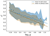 |
Fig. 4. 𝒞 versus log10χ. In blue, the results for the 𝒞 parameter computed on the mock Planck-like y-maps. In orange, the results for the 𝒞no_noise parameter computed on the mock y-maps generated without noise contamination (see Section 2.2.1). The blue triangles and the orange points are the mean values of 𝒞 and 𝒞no_noise, respectively, in each bin of log10χ. The shaded areas are at ±1σ. The solid blue line is the best linear fit of equation 𝒞 = (−0.24 ± 0.02) log10χ + (0.63 ± 0.01). The solid orange line is the best linear fit of equation 𝒞no_noise = (−0.29 ± 0.02) log10χ + (0.61 ± 0.01). |
As said before, the noise in the maps is a limiting factor when studying the morphology. Therefore, it is also interesting to see what is its impact on our analysis. Here, we also exploit the availability of mock y-maps realised for THE300 with the same angular resolution of Planck but without noise contamination. We refer to this ‘clean’ data set with a ‘no_noise’ sub-script. We applied the Zernike fit on these maps as well, following the same procedure above. For comparison, Fig. 3 also shows the cumulative distribution of THE300 clusters in this case (see the dashed grey line). It is evident that the impact of the noise is to increase the value of the 𝒞 parameter, with this effect being more pronounced in the left tails; namely, for the most regular maps. Again, we estimate the correlation 𝒞no_noise versus log10χ with a bootstrap method, obtaining 〈rno_noise〉=−0.47±0.02. In Fig. 4, in orange, we show 𝒞no_noise along log10χ. As for the previous case, the points are the mean value of 𝒞no_noise in each bin of log10χ and the shaded area is at ±1σ. The solid orange line is the best linear fit of Eq. (12), in which the best-fitting parameters are: a=−0.29±0.02 and b = 0.61±0.01. As expected, when neglecting the noise contamination in the maps the correlation between the inferred 2D morphology and the 3D dynamical state is higher. However, we notice that the two linear fits shown in Fig. 4 are compatible within 2σ. This means that the 𝒞 − log10χ relation remains poor sensitive to the noise features in the maps.
4.3. Dynamical state of Planck clusters
In the previous section, we verified that the sample of mock Planck-like y-maps generated for THE300 clusters is aptly representative, in terms of morphology, of the real Planck y-maps. The 𝒞 parameter estimated on these maps from the Zernike fit has a moderate linear correlation with the 3D dynamical indicator, χ. Then, the best linear fit resulting from this correlation (see Eq. (12)) can be used to deduce the relaxation parameter χ; namely, a proper dynamical state distribution, for the PSZ2_cosmo sample. For each Planck cluster, we solved the Eq. (12) for log10χ, using the best-fit parameters a and b estimated before. We applied a Monte-Carlo error propagation on these latter to compute the error on log10χ, using 104 random extractions from a 2D Gaussian distribution, accounting for the covariance between a and b. For each extraction, we compute the respective log10χ for each cluster. This generates a distribution of log10χ values for each cluster, from which we derive the median as well as the 16th and 84th percentiles. These values are reported in Table A.1.. We also constructed the histogram of the number of Planck clusters along log10χ for each random extraction, shown in Fig. 5. In each bin of log10χ, we have computed the mean number of clusters (i.e. the height of each bar) and the standard deviation (i.e. the error bar at the top). As described in Section 2.2.2, we applied the threshold log10χ>0 to recognise the relaxed clusters. By using the values reported in Table A.1., we estimated that the fraction of relaxed clusters in the PSZ2_cosmo sample is 61−66%.
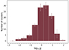 |
Fig. 5. Distribution of the number of Planck clusters along log10χ. The height of each bar is the mean number of clusters in the respective bin of log10χ and the error bar at the top is the standard deviation. |
We also analyse the distribution of log10χ values as a function of cluster mass, as shown in Fig. 6. The grey dashed lines indicate the mass bins considered and the pink dots represent the median of log10χ in each bin, with the error bars corresponding to the 16th and 84th percentiles. We notice a mild correlation, confirmed by computing the Pearson correlation coefficient (r = 0.41, p-value = 1.13×10⁻⁵), and the Spearman correlation coefficient (ρ = 0.49, p-value = 5.38×10⁻⁸). The correlation of the dynamical state of the clusters with their mass is not firmly established in the literature. Various studies, based on both observational data and simulations, have reported differing results. However, we note that some previous works analysing SZ samples found some indications that align with our findings. For instance, Rossetti et al. (2017) found a correlation, even if not strongly confirmed, between mass and cool-core fraction in a sample of clusters from the first release of the Planck catalogue (PSZ1; Planck Collaboration XX 2014). They found that the high-mass (>6.5×10¹⁴ M⊙) sub-sample features a higher fraction of cool-core clusters compared to the low-mass sub-sample, also noting that this was consistent with Mantz et al. (2015), who observed an increasing fraction of relaxed object with the temperature in SZ samples from Planck and SPT. However, both studies emphasised that the statistical significance of these results should be improved by considering larger samples. In contrast, Lovisari et al. (2017) and Bartalucci et al. (2019), who also analysed samples derived from Planck, did not find any evidence of a correlation between dynamical state and mass. Similarly, Campitiello et al. (2022) confirmed these results in their analysis of Planck clusters in the CHEX-MATE project (CHEX-MATE Collaboration 2021). However, upon examining Figure 2 of their study (and as noted by the authors themselves) after a visual classification of cluster maps, it appears that a larger fraction of relaxed object is found at low redshift (z<0.25) and with masses >4×10¹⁴ M⊙. On the other hand, simulation-based studies have reported opposite results, with evidence of higher fraction of relaxed objects among low-mass clusters (see e.g. Böhringer et al. 2010; Fakhouri et al. 2010). We also confirm this using our THE300 sample, where we found a weaker (∼30%) but opposite correlation between the log10χ values derived from the simulations and the masses. In this case, the more massive clusters appear more disturbed, consistent with previous results from Cui et al. (2018) and Santoni et al. (2024), who also analysed samples from THE300. These discrepancies between observations and simulations may be influenced by different biases, such as observational selection effects or the physical assumptions made in the simulations. We recall that our sample consists of a small number of nearby clusters, covering a mass range of ∼1−11×1014 M⊙; therefore, it is necessary to extend it to confirm a correlation between the dynamical state and mass (or otherwise).
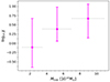 |
Fig. 6. Distribution of the dynamical state indicator, log10χ, as a function of cluster mass, M500. The grey dashed lines indicate the mass bins considered, while the pink dots mark the median value of log10χ in each bin, with error bars corresponding to the 16th and 84th percentiles. |
5. Comparison of the dynamical state classification with other works
The segregation of Planck clusters in terms of the dynamical state was already investigated using different morphological indicators based on multi-wavelength images. Each indicator refers to specific properties of cluster's components, such as gas or galaxies distribution, at different spatial scales. The net result is that the final definition of the state may not be unique. We believe that a fair comparison of the dynamical state definition of Planck clusters, inferred by standard indicators, with ZPs classification is useful to confirm (or otherwise) their identification. Therefore, we compare our results with previous works that already analysed sub-samples of galaxy clusters from the Planck catalogue. As pointed out in the literature, in the study of the dynamical state of galaxy clusters there is often no agreement on either the definition of the different classes into which the clusters are grouped (e.g. relaxed, most relaxed, disturbed, most disturbed, mixed, hybrid, and so on) or on the adopted parameters and thresholds for the classification. Also, the region used to study the clusters state (e.g. within R500, R200 or fraction of these) plays an important role in these analyses (De Luca et al. 2021). When adopting some of these criteria, several approaches are used to quantify their effectiveness. For example, estimating the completeness and/or the purity of the sample (Rasia et al. 2013; Lovisari et al. 2017; De Luca et al. 2021) or performing statistical tests to identify overlap between the distributions of the dynamical classes (Cialone et al. 2018; Lopes et al. 2018; De Luca et al. 2021) can help in characterizing the capabilities of the different classifications. It is also known that, in general, it is more simple to identify relaxed systems with respect to disturbed ones (Lovisari et al. 2017), for instance, due to projection effects.
In this work, we follow the approach in Lopes et al. (2018) to compare our results with the literature. We then computed the fraction of agreement, for relaxed clusters, between our dynamical classification and other works. Specifically, we compute the ratio between the number of clusters classified as relaxed both with log10χ and a specific parameter and the total number of relaxed clusters recognised with this latter. We report the results in Table 1. In the following, we describe the parameters used for the comparison and also the definition of 1relaxed cluster’ adopted in each work in more detail.
Agreement between the relaxation classification derived from ZPs and other indicators (third column) present in the literature (first column) for common cluster samples (the number of objects in the second column).
Rossetti et al. (2016) analysed the cosmology sample of clusters defined from the PSZ1 catalogue (Planck Collaboration XX 2014). As with the sample that we are taking into account here, their first sample was defined to maximise the completeness and the purity of the catalogue for cosmological analyses. The authors analysed Chandra, preferentially, and XMM-Newton observations for the selected clusters, and they used the offset between the BCG and the X-ray peak as indicator of the dynamical state. An offset less than 0.02R500 was used to identify relaxed clusters. We found 42 clusters in common with this sample and we estimate a fraction of agreement of 93–96%. The full sample in Rossetti et al. (2016) was extended to a higher redshift with respect to our selection, but they also used two halves, at low (<0.16) and high (>0.16) redshift, to study the possible evolution of the fraction of the relaxed clusters with the redshift. This type of study is beyond the aim of this paper due to the already mentioned angular resolution limitations; however, we notice that the fraction of relaxed clusters estimated in the low-redshift sub-sample (64%), which is almost the same redshift range we use here, is comparable with the fraction of relaxed clusters that we find in this work (61−66%).
Rossetti et al. (2017) reported a more detailed analysis done on the PSZ1 cosmology sample, with the aim of studying the cool-core state of the clusters. Even if this is a more specific question with respect to the characterisation of the dynamical state we are interested on, it is interesting to analyse the correlation with our results. The presence of a cool-core, in fact, is usually related to a relaxed state of the cluster, despite the fact that in some cases, a cool-core could be also present in a disturbed system (see e.g. Menanteau et al. 2012). The concentration parameter, c, is devoted to recognise cool-core systems by exploring the cluster cores, namely, regions within few hundred kpc from the cluster centre. With respect to our method that uses the ZPs within R500, it is more sensitive to the internal regions of the clusters. However, in C21, a good correlation (>80%) was found between the 𝒞 parameter from the Zernike fit and c, highlighting the advantage of this approach; that is, to explore large regions but in more details, being also sensitive to small scales by combining several functions. The c parameter was estimated in Rossetti et al. (2017) within 40 and 400 kpc from the cluster centre, using a threshold of 0.075 to recognise cool-core (c>0.075) and non cool-core (c<0.075) clusters. We refer to these two samples as relaxed and disturbed systems, respectively. Then, the fraction of agreement for the relaxed clusters is 86-88%.
Lovisari et al. (2017) studied the X-ray morphology of the Planck Early Sunyaev–Zel’dovich (ESZ) sample (Planck Collaboration VIII 2011), by using XMM-Newton images. They applied eight morphological parameters to classify the clusters dynamical state, analysing the performances of each parameter in terms of completeness and purity in revealing relaxed systems and using a previous visual classification as reference. We note that for the visual classification they use three classes: relaxed, disturbed, and mixed. They found that the best parameters to distinguish different dynamical states are the concentration, c, and the centroid shift, w. Therefore, we compare our results with only this two indicators. We note that in this case, the concentration parameter was computed in a more external region with respect to the application in Rossetti et al. (2017); namely, within 0.1R500 and R500. For the comparison with our results, as usual, we need to count the number of relaxed clusters identified by the single parameters in the reference work. Therefore, based on the discussion in Lovisari et al. (2017), we applied the thresholds that maximise the completeness for relaxed clusters on c and w. These latter were identified with c>0.15 and w<0.021. We found a fraction of agreement for relaxed clusters of 87–90% and 88%, respectively. The authors also highlighted that a combination of different parameters that are sensitive to different scales in the images can improve the morphological classification, as originally demonstrated in Rasia et al. (2013). This is in agreement with our discussion on the advantage of the multi-function Zernike fit. They also computed the combined parameter M as a function of c and w, but they did not provide the values of M for each cluster. Therefore, we limited our comparison to c and w only.
Andrade-Santos et al. (2017) analysed a sample of clusters from Planck ESZ as well, by using Chandra observations, but they focussed on the search of cool-core systems. They used four parameters well adapted to this aim: the concentration parameter, CSB4, computed in the internal cluster regions within 40 and 400 kpc and a modified version, indicated as CSB, where the regions analysed are scaled based on R500 of each cluster, namely, regions within 0.15R500 and R500; the cuspiness of the gas density profile, δ, computed at the radius equal to 0.04R500; the central gas density, ncore, computed at 0.01R500. As for the work of Rossetti et al. (2017), it is interesting to compare the results of our approach, that model the cluster maps within R500, with this analysis that takes into account more internal regions in the clusters. In addition, the sample used in Andrade-Santos et al. (2017) was also analysed in another work by Lopes et al. (2018) in which optical data are also used to segregate the clusters population. Therefore, the comparison with our work that uses tSZ maps is useful to draw a more complete picture of the analysis. However, note that we find a lower number of clusters in common with Lopes et al. (2018), since their analysis is limited in redshift by the optical surveys used, namely: the Sloan Digital Sky Survey, the 2dF Galaxy Redshift Survey and the 6dF Galaxy Survey. They used six optical estimators of the dynamical state, but they also suggest that the most reliable way to estimate the cluster state is by using the offset between BCG and X-ray centroid or the magnitude gap, Δm12, between the BCG and the second BCG. Therefore, we limit the comparison to these two parameters. Furthermore, Lopes et al. (2018) applied some statistical tests to derive the best thresholds for the parameters to separate the two populations of relaxed and disturbed systems (the same approach that has been recovered by Cialone et al. (2018) and De Luca et al. (2021)). In conclusion, they suggested that the thresholds used for the four parameters in Andrade-Santos et al. (2017) could be modified to have the best performance in the classification. We followed these results and in the comparison with the work of Andrade-Santos et al. (2017), we applied the new thresholds suggested for recognizing the relaxed clusters, namely, CSB>0.26, CSB4>0.055, δ>0.46, and ncore>8×10⁻³ cm−3. The thresholds for the offset and Δm12 are <0.01R500 and >1.0, respectively. The fractions of agreement with our work, for the relaxed clusters, are all larger than 74%.
Campitiello et al. (2022) studied the morphology of the 118 Planck clusters which compose the CHEX-MATE project (CHEX-MATE Collaboration 2021), a Multi-Year XMM-Newton Heritage Programme aimed at characterizing the statistical properties of the sample of most recent (0.05<z<0.2 with 2×10¹⁴ M⊙<M500<9×10¹⁴ M⊙) and most massive (z<0.6 with M500>7.25×10¹⁴ M⊙) clusters. They identified four parameters that, applied individually or combined together, can be used to recognise different dynamical classes: the concentration parameter, c, the centroid shift, w, and the second- and third-order power ratios, P20 and P30, all computed within R500. It is interesting to note that the power ratios are computed using a similar approach to the Zernike fit, by applying a multipole expansion to the surface brightness within a certain aperture. However, as already discussed in C21, the advantage of the Zernike modelling is the simultaneous use of several functions of different orders; due to their orthogonality, they can be easily combined. This allowed us to tune the modelling case by case in terms of the number of functions to use; namely, choosing the maximum order of the expansion based on the spatial scales one wants to recover. It also allowed us to adjust the modelling based on the noise contribution in the maps, as discussed in Section 3.1, whereas the contamination in the maps is known to be a limiting factor for the computation of the power ratios (Weißmann et al. 2013). In Campitiello et al. (2022), the authors also combined the four parameters above in a single indicator, M, which orders the clusters from the most relaxed to the most disturbed. This approach builds on the method introduced by Rasia et al. (2013) and has been employed in other studies, including the aforementioned Lovisari et al. (2017), as well as Cialone et al. (2018) and De Luca et al. (2021). However, the specific parameters combined and the adopted relationships differ across these works. Campitiello et al. (2022) highlighted that M provides a ranking of the clusters, namely, a continuous sequence based on the dynamical state, rather than a strict segregation in different classes. To test the efficiency of this method, they identified the clusters with lowest (highest) values of M and verify if these were classified as relaxed (disturbed) with a previous visual classification that is used as reference. However, they do not provide exacts values of M to identify these systems. They just considered the number of clusters classified as ‘most’ relaxed (disturbed) with the visual classification and select the same number of systems starting from the minimum (maximum) value of M. Then, they verified whether the two methods show an agreement for these clusters. The objects for which the two classifications match are indicated as relaxed or disturbed, with a mixed population within the two classes. Following these results, they provide a final rank of the clusters by ordering from the most relaxed (the first 15) to the most disturbed (the last 25) on the basis of M. Finally, the thresholds that they suggest for the single parameters are based on this strict classification; namely, they are values that allow us to recognise the most relaxed (disturbed) clusters classified both with M and visually. For the relaxed clusters, the thresholds are: c>0.49, w<0.006, P20<1.0×10⁻⁶, and P30<0.4×10⁻⁷. We note that these are values tighter with respect to the values used for the same parameters in the other works discussed above. This can explain the total agreement with our results, at least for the c and w, as reported in Table 1. On the contrary, the power ratios show the lower fraction. In particular with P20 there is the lowest mean agreement, while with P30 there is a large range between 58 and 100%. For the M parameter, we refer to the more general suggestion of considering M<0 to identify the fraction of relaxed systems to compare with our work.
To conclude, we verified that two clusters, PSZ2 G042.81+56.61 and PSZ2 G056.77+36.32, are in common with all the works considered above. Therefore, we checked whether they are classified in the same way with all the parameters reported in Table 1. We show the results in Fig. 7. The Planck y-maps analysed in this work are shown in the left panels, while in the plots on the right we indicate how the clusters are classified. We use the ‘relaxed’ caption to indicate if the cluster satisfies the thresholds reported above for the single parameters; otherwise, we refer to the more general class of ‘not relaxed’. Indeed, we note that some of the other works (see e.g. Lovisari et al. 2017; Campitiello et al. 2022) also define an intermediate group of ‘mixed’ clusters between the relaxed and the disturbed ones. We do not go into details of this more complex classification. With the χ parameter we classify both the clusters as relaxed (log10χ>0).
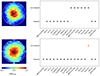 |
Fig. 7. Comparison of the dynamical state classification for PSZ2 G042.81+56.61 (PSZ2 index 156, top) and PSZ2 G056.77+36.32 (PSZ2 index 229, bottom) with the works mentioned in Section 5. Left: Planck y-maps analysed in this work for the two clusters. Right: Results of the dynamical state classification based on the papers and the parameters in Table 1 (see Section 5 for the thresholds applied to the single parameters to recognise relaxed clusters). |
For PSZ2 G042.81+56.61 (on the top in the figure), our result is in agreement with the X-ray classification in Rossetti et al. (2016, 2017), Lovisari et al. (2017), Andrade-Santos et al. (2017), but not with the optical analysis in Lopes et al. (2018). We note, as already mentioned, that for the parameters given in Andrade-Santos et al. (2017), we applied the thresholds suggested in Lopes et al. (2018). In Campitiello et al. (2022), the cluster does not satisfy the thresholds for the single parameters and it is not in the first 15 clusters that those authors identified as most relaxed. However, M=−0.05, therefore we indicate it as relaxed by using the less strict threshold we mentioned above (M<0).
PSZ2 G056.77+36.32 (bottom of the figure) is classified as relaxed with all the parameters, but P30 in Campitiello et al. (2022). However, we verified that the value of this parameter is 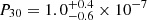 ; namely, the lower limit corresponds to the threshold that the authors indicated for the relaxed clusters (P30<0.4×10⁻⁷). Therefore, we indicate the results for this parameter in red in Fig. 7.
6. Conclusions
The study of the morphology of galaxy cluster maps is an observational approach that attempts to infer the dynamical state of these systems. In this work, we have conducted a morphological analysis using the Zernike polynomials, chosen for their straightforward analytical properties, which are well-suited for modelling circular cluster maps. This novel approach was introduced in Capalbo et al. (2021) for analysing mock high-angular resolution images of hydrodynamical simulated clusters from THE THREE HUNDRED project. Here, we apply the Zernike polynomials on real data for the first time. We analysed Compton parameter maps from the Planck satellite, focussing on galaxy clusters at z<0.1 due to the better resolution on mapping nearby systems. In particular, we modelled the maps within R500 for each cluster and we derived a single parameter, 𝒞, from the Zernike fit, to describe their morphology. The number of functions used for modelling must be tuned taking into account both the angular resolution of the maps and the noise spatial contamination. In this case, we chose the number of polynomials that would allow us to remain sensitive to the resolving scale of ∼2θ500. Mock maps were used to validate the analysis. These were generated for synthetic clusters in THE THREE HUNDRED project, resembling the real sample in terms of masses, redshift, signal-to-noise ratio, and 𝒞 parameter. The synthetic clusters were previously classified for their dynamical state, using a 3D indicator such as the relaxation parameter, χ. A linear correlation of approximately 38% was estimated between 𝒞 and log10χ for the simulated clusters. We note that this is a lower correlation, with respect to the results reported in Capalbo et al. (2021) (correlation >60% at z = 0), mainly due to the low angular resolution of the Planck maps and the noise contamination. Despite this limitation, we used this correlation to derive a distribution of the dynamical state of the real clusters in terms of χ. Then, a fraction of ∼63% of the clusters in the Planck sample were recognised as relaxed systems. The preliminary results of this study have been presented in Capalbo et al. (2024). The dynamical state classification derived in this work has also been compared with previous analyses in the literature conducted at different wavelengths and with different indicators. We note that some of those works also analysed the differences, in terms of dynamical state, between samples of clusters derived from SZ and X-ray surveys. This is beyond the aim of this paper and will be addressed in future works after the calibration of the Zernike modelling on X-ray data. As already mentioned, the proposed approach is subject to strong application limitations, such as where noise and angular resolution are of primary concern (as in Planck maps), restricting our analysis to nearby objects only. To address this challenge, we are applying the same method to higher resolution maps such as those from NIKA2 Sunyaev–Zel’dovich Large Program (Perotto et al. 2024). The application of Zernike polynomials is also promising on X-ray maps. Enjoying the reduced noise level and carefully choosing the number of polynomials in the modelling, it is possible to extend this method, as shown in the preliminary study of Capalbo et al. (2022). This approach is also being followed for the CHEX-MATE clusters.
Acknowledgments
The authors are grateful to the anonymous referee for the helpful comments and suggestions, which improved this work. This work has been made possible by THE THREE HUNDRED collaboration. The simulations used in this paper have been performed in the MareNostrum Supercomputer at the Barcelona Supercomputing Center, thanks to CPU time granted by the Red Española de Supercomputación. This work has received financial support from the European Union's Horizon 2020 Research and Innovation programme under the Marie Sklodowskaw-Curie grant agreement number 734374, i.e. the LACEGAL project. Some of the results in this paper have been derived using the HEALPY and HEALPIX packages. This research made use of POPPY, an open-source optical propagation Python package originally developed for the James Webb Space Telescope project (Perrin et al. 2012). VC, MDP and AF acknowledge financial support from PRIN-MIUR grant 20228B938N ”Mass and selection biases of galaxy clusters: a multi-probe approach” funded by the European Union Next generation EU, Mission 4 Component 1 CUP C53D2300092 0006 and from Sapienza Università di Roma, thanks to Progetti di Ricerca Medi 2022, RM1221816758ED4E. AF acknowledges the project ”Strengthening the Italian Leadership in ELT and SKA (STILES)”, proposal nr. IR0000034, admitted and eligible for funding from the funds referred to in the D.D. prot. no. 245 of August 10, 2022 and D.D. 326 of August 30, 2022, funded under the program ”Next Generation EU” of the European Union, “Piano Nazionale di Ripresa e Resilienza” (PNRR) of the Italian Ministry of University and Research (MUR), “Fund for the creation of an integrated system of research and innovation infrastructures”, Action 3.1.1 ”Creation of new IR or strengthening of existing IR involved in the Horizon Europe Scientific Excellence objectives and the establishment of networks”. WC is supported by the Atracción de Talento Contract no. 2020-T1/TIC-19882 granted by the Comunidad de Madrid in Spain and the science research grants from the China Manned Space Project. He also thanks the Ministerio de Ciencia e Innovación (Spain) for financial support under Project grant PID2021-122603NB-C21, ERC: HORIZON-TMA-MSCA-SE for supporting the LACEGAL-III project with grant number 101086388, and the science research grants from the China Manned Space Project with No. CMS-CSST-2021-A01, and CMS-CSST-2021-A03.
R500 is the radius enclosing an overdensity of 500 times the critical density of the Universe at cluster's redshift. A similar definition applies to the sub-script 200.
References
- Andrade-Santos, F., Jones, C., Forman, W. R., et al. 2017, ApJ, 843, 76 [Google Scholar]
- Bartalucci, I., Arnaud, M., Pratt, G. W., Démoclès, J., & Lovisari, L. 2019, A&A, 628, A86 [EDP Sciences] [Google Scholar]
- Beck, A. M., Murante, G., Arth, A., et al. 2016, MNRAS, 455, 2110 [Google Scholar]
- Bleem, L. E., Stalder, B., de Haan, T., et al. 2015, ApJS, 216, 27 [Google Scholar]
- Bleem, L. E., Bocquet, S., Stalder, B., et al. 2020, ApJS, 247, 25 [Google Scholar]
- Bleem, L. E., Crawford, T. M., Ansarinejad, B., et al. 2022, ApJS, 258, 36 [NASA ADS] [CrossRef] [Google Scholar]
- Böhringer, H., Pratt, G. W., Arnaud, M., et al. 2010, A&A, 514, A32 [NASA ADS] [CrossRef] [EDP Sciences] [Google Scholar]
- Buote, D. A., & Tsai, J. C. 1995, ApJ, 452, 522 [Google Scholar]
- Campitiello, M. G., Ettori, S., Lovisari, L., et al. 2022, A&A, 665, A117 [NASA ADS] [CrossRef] [EDP Sciences] [Google Scholar]
- Cao, K., Barnes, D. J., & Vogelsberger, M. 2021, MNRAS, 503, 3394 [NASA ADS] [CrossRef] [Google Scholar]
- Capalbo, V., De Petris, M., De Luca, F., et al. 2021, MNRAS, 503, 6155 [Google Scholar]
- Capalbo, V., De Petris, M., De Luca, F., et al. 2022, EPJ Web Conf., 257, 00008 [Google Scholar]
- Capalbo, V., De Petris, M., Cui, W., et al. 2024, EPJ Web Conf., 293, 00009 [Google Scholar]
- Carvalho, P., Rocha, G., & Hobson, M. P. 2009, MNRAS, 393, 681 [NASA ADS] [CrossRef] [Google Scholar]
- Carvalho, P., Rocha, G., Hobson, M. P., & Lasenby, A. 2012, MNRAS, 427, 1384 [CrossRef] [Google Scholar]
- Casas, M. C., Putnam, K., Mantz, A. B., Allen, S. W., & Somboonpanyakul, T. 2024, ApJ, 967, 14 [Google Scholar]
- Cerini, G., Cappelluti, N., & Natarajan, P. 2023, ApJ, 945, 152 [Google Scholar]
- CHEX-MATE Collaboration 2021, A&A, 650, A104 [NASA ADS] [CrossRef] [EDP Sciences] [Google Scholar]
- Cialone, G., De Petris, M., Sembolini, F., et al. 2018, MNRAS, 477, 139 [Google Scholar]
- Coulton, W., Madhavacheril, M. S., Duivenvoorden, A. J., et al. 2024, Phys. Rev. D, 109, 063530 [NASA ADS] [CrossRef] [Google Scholar]
- Cui, W., Power, C., Borgani, S., et al. 2017, MNRAS, 464, 2502 [NASA ADS] [CrossRef] [Google Scholar]
- Cui, W., Knebe, A., Yepes, G., et al. 2018, MNRAS, 480, 2898 [Google Scholar]
- de Andres, D., Cui, W., Ruppin, F., et al. 2022, Nat. Astron., 6, 1325 [NASA ADS] [CrossRef] [Google Scholar]
- De Luca, F., De Petris, M., Yepes, G., et al. 2021, MNRAS, 504, 5383 [NASA ADS] [CrossRef] [Google Scholar]
- Fakhouri, O., Ma, C. -P., & Boylan-Kolchin, M. 2010, MNRAS, 406, 2267 [CrossRef] [Google Scholar]
- Giodini, S., Lovisari, L., Pointecouteau, E., et al. 2013, Space Sci. Rev., 177, 247 [Google Scholar]
- Gorski, K. M., Hivon, E., Banday, A. J., et al. 2005, ApJ, 622, 759 [Google Scholar]
- Haggar, R., Gray, M. E., Pearce, F. R., et al. 2020, MNRAS, 492, 6074 [NASA ADS] [CrossRef] [Google Scholar]
- Hilton, M., Hasselfield, M., Sifón, C., et al. 2018, ApJS, 235, 20 [Google Scholar]
- Hilton, M., Sifón, C., Naess, S., et al. 2021, ApJS, 253, 3 [Google Scholar]
- Huang, N., Bleem, L. E., Stalder, B., et al. 2020, AJ, 159, 110 [Google Scholar]
- Hudson, D. S., Mittal, R., Reiprich, T. H., et al. 2010, A&A, 513, A37 [NASA ADS] [CrossRef] [EDP Sciences] [Google Scholar]
- Hurier, G., Macías-Pérez, J. F., & Hildebrandt, S. 2013, A&A, 558, A118 [NASA ADS] [CrossRef] [EDP Sciences] [Google Scholar]
- Jones, C., & Forman, W. 1984, ApJ, 276, 38 [NASA ADS] [CrossRef] [Google Scholar]
- Jones, C., & Forman, W. 1992, in Clusters and Superclusters of Galaxies, ed. A. C. Fabian, NATO Advanced Study Institute (ASI) Series C, 366, 49 [NASA ADS] [CrossRef] [Google Scholar]
- Kaiser, N. 1986, MNRAS, 222, 323 [Google Scholar]
- Klypin, A., Yepes, G., Gottlöber, S., Prada, F., & Heß, S. 2016, MNRAS, 457, 4340 [Google Scholar]
- Knollmann, S. R., & Knebe, A. 2009, ApJS, 182, 608 [Google Scholar]
- Kravtsov, A. V., & Borgani, S. 2012, ARA&A, 50, 353 [Google Scholar]
- Lavoie, S., Willis, J. P., Démoclès, J., et al. 2016, MNRAS, 462, 4141 [NASA ADS] [CrossRef] [Google Scholar]
- Li, Q., Han, J., Wang, W., et al. 2022, MNRAS, 514, 5890 [Google Scholar]
- Lopes, P. A. A., Trevisan, M., Laganá, T. F., et al. 2018, MNRAS, 478, 5473 [Google Scholar]
- Lovisari, L., Forman, W. R., Jones, C., et al. 2017, ApJ, 846, 51 [Google Scholar]
- Mahajan, V. N. 2007, in Polynomial and Wavefront Fitting, 3rd edn., ed. M. D. Zernike (New Jersey: John Wiley & Sons, Inc.), 498–546 [Google Scholar]
- Mantz, A. B., Allen, S. W., Morris, R. G., et al. 2015, MNRAS, 449, 199 [CrossRef] [Google Scholar]
- Melin, J. B., Bartlett, J. G., & Delabrouille, J. 2006, A&A, 459, 341 [NASA ADS] [CrossRef] [EDP Sciences] [Google Scholar]
- Melin, J. -B., Aghanim, N., Bartelmann, M., et al. 2012, A&A, 548, A51 [NASA ADS] [CrossRef] [EDP Sciences] [Google Scholar]
- Menanteau, F., Hughes, J. P., Sifón, C., et al. 2012, ApJ, 748, 7 [NASA ADS] [CrossRef] [Google Scholar]
- Mohr, J. J., Fabricant, D. G., & Geller, M. J. 1993, ApJ, 413, 492 [Google Scholar]
- Mroczkowski, T., Nagai, D., Basu, K., et al. 2019, Space Sci. Rev., 215, 17 [Google Scholar]
- Niu, K., & Tian, C. 2022, J. Opt., 24, 123001P [Google Scholar]
- Noll, R. J. 1976, J. Opt. Soc. Am., 66, 207 [Google Scholar]
- O’Hara, T. B., Mohr, J. J., Bialek, J. J., & Evrard, A. E. 2006, ApJ, 639, 64 [Google Scholar]
- Parekh, V., van der Heyden, K., Ferrari, C., Angus, G., & Holwerda, B. 2015, A&A, 575, A127 [NASA ADS] [CrossRef] [EDP Sciences] [Google Scholar]
- Perotto, L., Adam, R., Ade, P., et al. 2024, EPJ Web Conf., 293, 00040 [Google Scholar]
- Perrin, M. D., Soummer, R., Elliott, E. M., Lallo, M. D., & Sivaramakrishnan, A. 2012, in Space Telescopes and Instrumentation 2012: Optical, Infrared, and Millimeter Wave, eds. M. C. Clampin, G. G. Fazio, H. A. MacEwen, J. Oschmann, & M. Jacobus, SPIE Conf. Ser., 8442, 84423D [Google Scholar]
- Planck Collaboration VIII. 2011, A&A, 536, A8 [NASA ADS] [CrossRef] [EDP Sciences] [Google Scholar]
- Planck Collaboration XX. 2014, A&A, 571, A20 [NASA ADS] [CrossRef] [EDP Sciences] [Google Scholar]
- Planck Collaboration XIII. 2016, A&A, 594, A13 [NASA ADS] [CrossRef] [EDP Sciences] [Google Scholar]
- Planck Collaboration XXII. 2016, A&A, 594, A22 [NASA ADS] [CrossRef] [EDP Sciences] [Google Scholar]
- Planck Collaboration XXIV. 2016, A&A, 594, A24 [NASA ADS] [CrossRef] [EDP Sciences] [Google Scholar]
- Planck Collaboration XXVII. 2016, A&A, 594, A27 [NASA ADS] [CrossRef] [EDP Sciences] [Google Scholar]
- Planck Collaboration VI. 2020, A&A, 641, A6 [NASA ADS] [CrossRef] [EDP Sciences] [Google Scholar]
- Pratt, G. W., Arnaud, M., Biviano, A., et al. 2019, Space Sci. Rev., 215, 25 [Google Scholar]
- Rasia, E., Meneghetti, M., & Ettori, S. 2013, Astron. Rev., 8, 40 [Google Scholar]
- Remazeilles, M., Delabrouille, J., & Cardoso, J. -F. 2011, MNRAS, 410, 2481 [CrossRef] [Google Scholar]
- Ribeiro, A. L. B., Lopes, P. A. A., & Rembold, S. B. 2013, A&A, 556, A74 [NASA ADS] [CrossRef] [EDP Sciences] [Google Scholar]
- Rigaut, F., Rousset, G., Kern, P., et al. 1991, A&A, 250, 280 [NASA ADS] [Google Scholar]
- Rossetti, M., Gastaldello, F., Ferioli, G., et al. 2016, MNRAS, 457, 4515 [Google Scholar]
- Rossetti, M., Gastaldello, F., Eckert, D., et al. 2017, MNRAS, 468, 1917 [Google Scholar]
- Ruppin, F., Sembolini, F., De Petris, M., et al. 2019, A&A, 631, A21 [NASA ADS] [CrossRef] [EDP Sciences] [Google Scholar]
- Santoni, S., De Petris, M., Yepes, G., et al. 2024, A&A, 692, A44 [NASA ADS] [CrossRef] [EDP Sciences] [Google Scholar]
- Santos, J. S., Rosati, P., Tozzi, P., et al. 2008, A&A, 483, 35 [NASA ADS] [CrossRef] [EDP Sciences] [Google Scholar]
- Schade, D., Lilly, S. J., Crampton, D., et al. 1995, ApJ, 451, L1 [NASA ADS] [CrossRef] [Google Scholar]
- Seppi, R., Comparat, J., Nandra, K., et al. 2023, A&A, 671, A57 [NASA ADS] [CrossRef] [EDP Sciences] [Google Scholar]
- Staniszewski, Z., Ade, P. A. R., Aird, K. A., et al. 2009, ApJ, 701, 32 [CrossRef] [Google Scholar]
- Sunyaev, R. A., & Zeldovich, Y. B. 1972, Comments Astrophys. Space Phys., 4, 173 [NASA ADS] [EDP Sciences] [Google Scholar]
- Svechnikov, M., Chkhalo, N., Toropov, M., & Salashchenko, N. 2015, Optics Express, 23, 14677 [Google Scholar]
- Vikhlinin, A., Burenin, R., Forman, W. R., et al. 2007, in Heating versus Cooling in Galaxies and Clusters of Galaxies, eds. H. Böhringer, G. W. Pratt, A. Finoguenov, & P. Schuecker, 48 [Google Scholar]
- Voit, G. M. 2005, Rev. Mod. Phys., 77, 207 [Google Scholar]
- Weißmann, A., Böhringer, H., Šuhada, R., & Ameglio, S. 2013, A&A, 549, A19 [NASA ADS] [CrossRef] [EDP Sciences] [Google Scholar]
- Wen, Z. L., & Han, J. L. 2013, MNRAS, 436, 275 [Google Scholar]
- Zernike, F. 1934, MNRAS, 94, 377 [Google Scholar]
- Zhang, B., Cui, W., Wang, Y., Dave, R., & De Petris, M. 2022, MNRAS, 516, 26 [NASA ADS] [CrossRef] [Google Scholar]
- Zonca, A., Singer, L. P., Lenz, D., et al. 2019, J. Open Source Softw., 4, 1298 [NASA ADS] [CrossRef] [Google Scholar]
Appendix A: Morphological and dynamical state parameters
The morphological parameter, 𝒞, derived from the Zernike fit and the deduced dynamical state indicator, log10χ, for the selected Planck clusters are reported in Table A.1.. The parameters are calculated within R500.
𝒞 and log10χ for the selected 109 Planck clusters at z<0.1, listed with index and PSZ2 name.
Continued.
All Tables
Agreement between the relaxation classification derived from ZPs and other indicators (third column) present in the literature (first column) for common cluster samples (the number of objects in the second column).
𝒞 and log10χ for the selected 109 Planck clusters at z<0.1, listed with index and PSZ2 name.
All Figures
|
Fig. 1. Distribution in the M500−z plane of 109 Planck-SZ clusters (red triangles) selected for the morphological analysis (see Section 2.1). The thin dashed vertical lines mark the redshift bins used for the comparison with the synthetic clusters (grey dots) from THE300 project (see Section 2.2). In the right panel, we give the normalised distributions of the masses for the Planck (in red) and THE300 (in grey) samples. |
| In the text | |
|
Fig. 2. Left: Examples of Planck y-maps of three clusters with different values of the 𝒞 parameter. Top: cluster PSZ2 G075.71+13.51 (PSZ2 index 322). Middle: cluster PSZ2 G340.88−33.36 (PSZ2 index 1591). Bottom: cluster PSZ2 G093.94−38.82 (PSZ2 index 430). Each map is centred on the cluster position reported in the PSZ2 catalogue, with side-length equal to 2θ500. The white circle is the aperture defined for the Zernike fit. The markers in green in the top-right corner of each map are used to indicate the respective values of the 𝒞 parameter in Fig. 3. Right: Bar charts of the cn,±m coefficients (see Eq. (11)) resulting from the Zernike fit applied on each map on the left. The ZPs on the x axis are ordered following the Noll's scheme (Noll 1976). The polynomial order n increases from left to right. Orange and blue bars refer to ZPs with m = 0 and m≠0, respectively. |
| In the text | |
|
Fig. 3. Cumulative distribution of the number of clusters along the 𝒞 parameter. The red line refers to the PSZ2_cosmo sample, the grey lines refer to the sample selected from THE300, and considering, respectively, their Planck-like maps (solid line) and their maps without noise (dashed line). The green markers are used to indicate the value of 𝒞 for the three maps shown in Fig. 2. |
| In the text | |
|
Fig. 4. 𝒞 versus log10χ. In blue, the results for the 𝒞 parameter computed on the mock Planck-like y-maps. In orange, the results for the 𝒞no_noise parameter computed on the mock y-maps generated without noise contamination (see Section 2.2.1). The blue triangles and the orange points are the mean values of 𝒞 and 𝒞no_noise, respectively, in each bin of log10χ. The shaded areas are at ±1σ. The solid blue line is the best linear fit of equation 𝒞 = (−0.24 ± 0.02) log10χ + (0.63 ± 0.01). The solid orange line is the best linear fit of equation 𝒞no_noise = (−0.29 ± 0.02) log10χ + (0.61 ± 0.01). |
| In the text | |
|
Fig. 5. Distribution of the number of Planck clusters along log10χ. The height of each bar is the mean number of clusters in the respective bin of log10χ and the error bar at the top is the standard deviation. |
| In the text | |
|
Fig. 6. Distribution of the dynamical state indicator, log10χ, as a function of cluster mass, M500. The grey dashed lines indicate the mass bins considered, while the pink dots mark the median value of log10χ in each bin, with error bars corresponding to the 16th and 84th percentiles. |
| In the text | |
|
Fig. 7. Comparison of the dynamical state classification for PSZ2 G042.81+56.61 (PSZ2 index 156, top) and PSZ2 G056.77+36.32 (PSZ2 index 229, bottom) with the works mentioned in Section 5. Left: Planck y-maps analysed in this work for the two clusters. Right: Results of the dynamical state classification based on the papers and the parameters in Table 1 (see Section 5 for the thresholds applied to the single parameters to recognise relaxed clusters). |
| In the text | |
Current usage metrics show cumulative count of Article Views (full-text article views including HTML views, PDF and ePub downloads, according to the available data) and Abstracts Views on Vision4Press platform.
Data correspond to usage on the plateform after 2015. The current usage metrics is available 48-96 hours after online publication and is updated daily on week days.
Initial download of the metrics may take a while.