| Issue |
A&A
Volume 698, June 2025
|
|
|---|---|---|
| Article Number | A286 | |
| Number of page(s) | 19 | |
| Section | Interstellar and circumstellar matter | |
| DOI | https://doi.org/10.1051/0004-6361/202452397 | |
| Published online | 23 June 2025 | |
Unmasking the physical information inherent to interstellar spectral line profiles with machine learning
I. Application of LTE to HCN and HNC transitions
1
Dept. Ciencias Integradas, Facultad de Ciencias Experimentales, Centro de Estudios Avanzados en Física, Matemática y Computación, Unidad Asociada GIFMAN, CSIC-UHU, Universidad de Huelva,
Spain
2
Lyon College,
Batesville,
AR,
USA
3
Planetário Juan Bernardino Marques Barrio, Instituto de Estudos Socioambientais, Universidade Federal de Goiás,
Brazil
4
Centro de Estudios Avanzados en Física, Matemática y Computación, Universidad de Huelva,
Spain
5
Andalusian Research Institute in Data Science and Computational Intelligence, Universidad de Huelva,
Spain
6
Dept. Tecnologías de la Información, Escuela Técnica Superior de Ingeniería, Centro de Estudios Avanzados en Física, Matemática y Computación, Universidad de Huelva,
Spain
7
SRON Netherlands Institute for Space Research & Kapteyn Astronomical Institute, University of Groningen,
9747 AD
Groningen,
The Netherlands
8
Instituto Universitario Carlos I de Física teórica y computacional, Universidad de Granada,
Spain
★ Corresponding authors: This email address is being protected from spambots. You need JavaScript enabled to view it.
; This email address is being protected from spambots. You need JavaScript enabled to view it.
Received:
27
September
2024
Accepted:
25
April
2025
Abstract
Context. Physical and chemical properties, such as kinetic temperature, volume density, and molecular composition of interstellar clouds are inherent in their line spectra at submillimeter wavelengths. Therefore, the spectral line profiles could be used to estimate the physical conditions of a given source.
Aims. We present a new bottom-up approach, based on machine learning (ML) algorithms, to extract the physical conditions in a straightforward way from the line profiles without using radiative transfer equations.
Methods. We simulated, for the typical physical conditions of dense molecular clouds and star-forming regions, the emission in spectral lines of the two isomers HCN and HNC, from J = 1–0 to J = 5–4 between 30 and 500 GHz, which are commonly observed in dense molecular clouds and star forming regions. The generated data cloud distribution has been parametrised using the line intensities and widths to enable a new way to analyse the spectral line profiles and to infer the physical conditions of the region. The line profile parameters have been charted to the HNC/HCN ratio and the excitation temperature of the molecule(s). Three ML algorithms have been trained, tested, and compared aiming to unravel the excitation conditions of HCN and HNC and their abundance ratio.
Results. Machine learning results obtained with two spectral lines, one for each isomer HCN and HNC, have been compared with the local thermodynamic equilibrium (LTE) analysis for the cold source R CrA IRS 7B. The estimate of the excitation temperature and of the abundance ratio, in this case considering the two spectral lines, is in agreement with our LTE analysis. The complete optimisation procedure of the algorithms (training, testing, and prediction of the target quantities) have the potential to predict interstellar cloud properties from line profile inputs at lower computational cost than before.
Conclusions. It is the first time that the spectral line profiles are mapped according to the physical conditions charting the ratio of two isomers and the excitation temperature of the molecules. In addition, a bottom-up approach starting from a set of simulated spectral data at different physical conditions is proposed to interpret line observations of interstellar regions and to estimate their physical conditions. This new approach presents the potential relevance to unravel hidden interstellar conditions with the use of ML methods.
Key words: astrochemistry / molecular data / methods: data analysis / methods: miscellaneous / ISM: molecules
© The Authors 2025
 Open Access article, published by EDP Sciences, under the terms of the Creative Commons Attribution License (https://creativecommons.org/licenses/by/4.0), which permits unrestricted use, distribution, and reproduction in any medium, provided the original work is properly cited.
This article is published in open access under the Subscribe to Open model. This email address is being protected from spambots. You need JavaScript enabled to view it. to support open access publication.
1 Introduction
The physical properties of the gas in the Interstellar Medium (ISM), including temperature, density, molecular composition, and abundance, can be determined from the characterisation of the molecular spectra of infrared and radio line surveys (Shaw 2006; Draine 2011; McGuire et al. 2020; Cernicharo et al. 2023). This characterisation is achieved, first and foremost, by ongoing efforts to measure and analyse molecular spectra in the laboratory (Pickett et al. 1998; Carvajal et al. 2009; Endres et al. 2016) and to derive the required spectroscopic quantities, such as line strengths, rovibrational energies, and internal partition functions (Carvajal et al. 2010; Roueff & Lique 2013; Lefloch et al. 2018; Mendoza et al. 2018; van der Tak et al. 2020; Mendoza et al. 2023; Carvajal et al. 2019, 2024). Thus, from the conditions in the laboratory, assumed under control, to conditions in the ISM of galaxies, the spectral lines can be extrapolated allowing us to determine the physical conditions of the regions. Nevertheless, the ISM spectral lines stack a huge amount of information about the physical conditions of the source and of the observation techniques. In fact, the profiles of the spectral lines observed in an ISM survey contain an information richer than the one intrinsic of each molecule – coming from the quantum mechanical properties enclosed by the molecule itself – measured in the lab, in particular, the physical conditions of the surveyed objects and of the observations: excitation temperature (Tex), abundance ratio, source’s size (θ), and linewidths (ΔVsys) (van der Tak et al. 2007, 2020; McGuire et al. 2021). Therefore, in molecular astronomy and astrochemistry, the physical and molecular properties of the observed sources are inherent in each spectral line profile, although they are hidden in the quantities involved in the transition. Conventionally, by means of radiative transfer methods, it is possible to infer the physical properties from astronomical maps and line surveys (Holdship et al. 2022).
In this work, we propose a new approach, based on machine learning (ML) algorithms, to extract the physical conditions in a straightforward way from the spectral line profiles, without using radiative transfer equations. The process followed by us is the same that was recently suggested for the application of ML in astronomy (Buchner & Fotopoulou 2024). In particular, our work addresses to determine fundamental quantities in astrochemistry as the temperatures and column densities in the ISM (Draine 2011; Jørgensen et al. 2020), exploiting, with the use of ML algorithms, the spectral properties of molecular lines. Previously, Gratier et al. (2021) evaluated the use of radio molecular line observations, including CO isotopologues, HCO+, N2H+, and CH3OH, to predict H2 column densities through ML methods such as random forest. Bron et al. (2021) presented a general method based on a grid of models covering the full range of possible values for unknown physical parameters, such as gas density, temperature, and depletion, to identify tracers of the ionisation fraction in dense and translucent gas using random forest.
We here focused on the molecules hydrogen cyanide (HCN) and hydrogen isocyanide (HNC), which are among the most abundant isomers in dense molecular clouds. They play a crucial role in the chemistry of molecular clouds and are regarded as precursors of complex molecules like the nucleobase adenine (Jung & Choe 2013). Although HCN is more stable than HNC because of its lower potential minimum (Khalouf-Rivera et al. 2019; Zamir & Stein 2022), the isomerisation between HCN and HNC is a key reaction in astrochemistry, driven by quantum tunnelling and thermodynamic factors. Recent studies employing ML techniques have successfully predicted the reactivity boundaries of this isomerisation without using the classical reaction dynamics theory (Yamashita et al. 2023). The interconversion between HCN and HNC can occur both in the gas phase and on icy grain surfaces under the distinct conditions of the ISM. Studies indicates that their abundances can be influenced by various physicochemical factors (e.g., Mendes et al. 2012; Graninger et al. 2014; Baiano et al. 2022). Consequently, the isomeric ratios of HCN to HNC can offer valuable insights into the evolution and properties of interstellar objects. From observations in infrared to submillimeter wavelengths, the detection of both isomers in star-forming regions at various evolutionary stages is well-documented. Recent findings on 12C/13C ratios have been obtained from far-infrared observations of HNC and H13CN in the hot core Orion IRc2 (Nickerson et al. 2021). Additionally, the isomeric ratios and isotopic fractionation of HCN and HNC have been discussed for their role as a chemical clock, providing insights about the chemical evolution of star-forming regions at different stages (e.g., Jin et al. 2015; Pazukhin et al. 2023). Early studies of the Orion KL hot core combining observational and experimental data revealed that the HNC/HCN ratio decreases with a rising temperature and density (Schilke et al. 1992; Tachikawa et al. 2003). Hacar et al. (2020) analysed the intensity ratios of the J = 1–0 lines of HCN and HNC across the Integral Shape Filament in Orion, correlating them with the gas kinetic temperature. Empirical linear fit calibrations were developed for regimes of low-temperature (TK < 40 K) and high-temperature (TK ≳ 40 K). HNC generally traces cold environments (10 K), but in hot regions, its presence is believed from active ion-molecule chemistry and infrared pumping. Pérez-Beaupuits et al. (2007) discussed this scenario through the analysis of HCN and HNC 3–2 transitions in several Seyfert galaxies. In the ultra-luminous Infrared Galaxy IRAS 20551-4250, Imanishi et al. (2017) used ALMA observations of HCN, HNC and HCO+ to analyse their excitation conditions and implications for infrared radiative pumping.
The study of the ISM relies heavily on the accurate modelling of the physical and chemical properties of detected molecules. In the literature, various methods have been developed to estimate physical properties using observational data and computational techniques. Among these, sampling methods–particularly Bayesian inference – have proven to be statistically robust. For instance, nested sampling has been applied to chemical and radiative transfer models (Behrens et al. 2022). Sequential Monte Carlo samplers and Markov Chain Monte Carlo (MCMC) methods have been used to study the evolution of interstellar dust in the context of galaxies (Galliano et al. 2021; Ramambason et al. 2022). Additionally, MCMC has been employed to analyse spectral data from sources such as TMC-1 (Gratier et al. 2016), while sequential Monte Carlo methods have been applied in other astrophysical contexts (Lebouteiller & Ramambason 2022). Spectroscopic data analysis has also benefited from methods such as minimum χ2 fitting (Joblin et al. 2018) and gradient-based algorithms (Paumard et al. 2022). Furthermore, similar techniques have been utilised earlier (Galliano et al. 2003). Traditionally, local thermodynamic equilibrium (LTE) models have provided a simplified, yet effective approach for characterising excitation conditions due to their computational feasibility and broad applicability across a wide range of molecules and transitions. In this work, we present the first generalised framework for developing and validating ML methods to predict parameters of astrochemical and astrophysical interest under LTE conditions.
The problem has been defined to derive two outcomes from the algorithms – excitation temperatures and the HNC/HCN ratios – using a dataset that integrates synthetic and semi-empirical data, combining LTE models with observations, as detailed in subsequent sections. Given the complexities involved in data handling, we focus on the versatile case of interstellar tracers HCN and HNC to calibrate and evaluate different ML algorithms under LTE conditions. The use of LTE models allows the spectral simulations and analysis to incorporate numerous inputs and variables associated with spectroscopy and observational parameters – namely, transition lines, rest frequencies, systemic velocities, angular and spectral resolution – while it also enables the generation of a manageable synthetic dataset for training and testing algorithms. Although this approach introduces a bias by restricting the study to LTE-based assumptions (Roueff et al. 2024) and only a subset of molecules (two out of over 300 known in the ISM), our defined problem and workflow are structured to allow for the future expansion of hypotheses, inclusion of additional molecular species, and adaptation to more complex data treatments.
The accuracy of predictions made by neural networks, artificial intelligence, and ML methods depends notably on the volume and quality of the data used during the training (Delli Veneri et al. 2023; Priestley et al. 2023). Thus, with the purpose of introducing this new approach, first we simulated LTE spectral line profiles of the isomers HCN and HNC according to the ISM physical conditions across a broad range of temperatures (Texc=5–150 K), frequencies (v=30–500 GHz) and other quantities. The profiles data, fitted as Gaussian functions, have been parametrised considering the line intensities and widths, generating a data cloud distribution for an initial analysis of the data set. Then we assessed three different ML algorithms using semi-empirical lines, derived from archival data from single-dish telescopes (e.g., IRAM-30m and APEX) alongside LTE models, in the excitation conditions of the Orion KL hot core as a reference. Afterwards a realistic system such as R CrA IRS 7B, which is a cold source in the R Corona Australis star-forming region, has been tackled for testing this approach in a realistic scenario using observed spectra. For this latter case, we estimated the excitation temperature and the HNC/HCN ratio and they have been compared with the results obtained from LTE analysis obtained in this work. This work represents a preliminary contribution given the multiple questions that raise in the application of this new approach when the level of complexity – related to the spectroscopy, radiative scenarios, instruments, and astronomical sources – increases (van der Tak 2011; Martin et al. 2021; Nyheim et al. 2024).
This article is organised as follows: Section 2 describes the methodology of the proposed novel approach, detailing the ML algorithms employed, the LTE spectral models, and the data processing of the observations obtained from the ESO archive. Section 3 discusses the predictions of the approach on semi-empirical data from a representative hot core. In addition, this approach is applied to the R CrA IRS 7B source and its results are compared with those obtained from a mainstream method. Section 5 draws the conclusions of this novel approach.
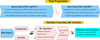 |
Fig. 1 Schematic of the workflow for training and evaluating ML models to predict excitation temperatures and isomeric ratios from HCN and HNC spectra. Data preparation integrates models and observations to build a dataset. Gaussian fit parameters are used to generate a data cloud of line intensity vs. width, gradient-tagged by temperatures and ratios. Training and testing stages utilise three algorithms, with results benchmarked against radiative transfer models and validated using observational prototype data. |
2 Methodology
In this section, we explore the effect of the physical conditions on the profiles of submillimeter lines and we make the most of this analysis to estimate the HNC/HCN ratios and the excitation temperature of a source with the use of ML algorithms. Although this study can be addressed considering any molecule, we considered the spectral lines from J = 1–0 to J = 5–4 of the two isomers HCN and HNC. These two isomers were detected in many sources and have been proven suitable to determine the gas temperature and the evolution of interstellar objects (Schilke et al. 1992; Hacar et al. 2020). They are good candidates for a comprehensive analysis of the spectral line profiles in the study of the ISM and, in particular, when ML is going to be applied.
We outlined here the methodology employed to estimate the physical conditions of an interstellar source. Fig. 1 presents the workflow of the proposed bottom-up approach, which encompasses the two followed steps: data preparation and ML predictions of quantities relevant to astrophysical research. The first step, as described in Sect. 2.1, involves the simulation of the spectral lines under different physical conditions. To do so, models were carried out under LTE hypotheses obtaining as outputs spectral lines following Gaussian distributions. A key aspect of our approach is the decision to adopt LTE. While this choice is a source of bias, it was strategically selected to establish a controlled baseline for the ML development. These simulations serve to parametrise their spectral profiles and facilitate a comprehensive analysis of the simulated data. In the second step, ML algorithms are trained using the simulated data for estimating the physical conditions of the interstellar source. In this first article, particular attention is given to the HNC/HCN ratios and their excitation temperatures under LTE conditions. The ML methods utilised in this work are outlined in Sect. 2.2. This methodology is developed using synthetic spectra derived from LTE models and semi-empirical data, which integrates LTE simulations with observed spectral lines. It also includes an evaluation based on observational data collected with the APEX telescope towards the R CrA IRS 7B source, with the data reduction and analysis detailed in Sect. 2.3.
2.1 Simulation, parametrisation and analysis of the spectral line profiles
We generated an extensive set of synthetic spectra for HCN and HNC, approximately 3 × 10⁵ spectra, employing Gaussian line profiles as the basis for their generation. These were produced using a comprehensive grid of physical parameters pivotal for modelling spectral line profiles, including excitation temperatures, linewidths, HNC/HCN ratios, and source sizes. The compilation of the synthetic spectra at different ISM conditions is tackled with the parametrisation of each spectral line through the intensity I (K) and the linewidth Δv (MHz). This latter is related to the linewidth at half intensity (FWHM = 2  Δv), which is named ΔVsys when expressed in km s−1. This set of parameters (I, Δv) is compiled in a data cloud aimed to visualise the data distribution according to the physical conditions. The ML approach will estimate the physical conditions of a ISM source from the data distribution obtained from a thorough and comprehensive set of simulated spectral lines. This is contrary to the top-down mainstream approaches (e.g., the population diagram analysis of molecular spectral lines considering the LTE approximation Goldsmith & Langer 1999 or the application of the non-LTE radiative transfer RADEX code van der Tak et al. 2007), which derive the physical parameters of the observed regions from the characterisation of a limited number of identified spectral lines. In this work we propose a bottom-up approach to obtain the ISM physical conditions from the observed lines, using ML techniques and analyses based on synthetic spectra generated beforehand (see Fig. 1). Therefore, this new approach has a more general scope because, when the spectral lines simulations are carried out, it is conceived to determine the physical parameters to a set of observed sources all at once.
The grid of the synthetic spectral lines has been generated using GILDAS1 and CASSIS2 software, adopting LTE conditions. Hence, the molecule energy levels are assumed populated according to the Boltzmann distribution and the excitation temperature (Texc), associated with a particular molecular transition, is equal to the gas kinetic temperature. This can be determined from the ratio of the population or column densities between two energy levels, i and j, characterised by their statistical weights, gi and gj, and the corresponding energies, Ei and Ej, by
![Mathematical equation: $\frac{N_{j}}{N_{i}}=\frac{g_{j}}{g_{i}} \exp \left[\frac{-\left(E_{j}-E_{i}\right)}{k T_{\text{exc}}}\right].$](/articles/aa/full_html/2025/06/aa52397-24/aa52397-24-eq2.png) (1)
(1)
In contrast, under non-LTE conditions, an accurate estimate of the kinetic temperature requires to consider collisional processes and to solve statistical equilibrium equations (Goldsmith & Langer 1999; van der Tak et al. 2007; Shirley 2015).
As the local properties of the gas are assumed in thermal equilibrium, a Gaussian curve is used to describe the shape of the spectral lines in the observed frequency range. This profile is associated with thermal broadening due to the random motion of molecules – specifically HCN and HNC in this case – within the gas, leading to a characteristic velocity distribution that produces the observed spectral line shape (e.g. Roueff et al. 2021 and references therein). Thus we can also justify the use of Gaussian fits to parametrise the simulated spectral line profiles and, in particular, to relate them with the column density of the upper level involved in the transitions and the excitation temperature. In this study, we performed the simulations for the ten spectral lines J = 1–0 (around 90 GHz), J = 2–1(∼180 GHz), J = 3–2 (∼ 270 GHz), J = 4–3 (∼360 GHz), and J = 5–4 (∼450 GHz) of HCN and HNC at temperatures from 5 K to 150 K in steps of 5 K, abundance ratios HNC/HCN for the set of values from 0.1 to 1.0 in steps of 0.1, source’s sizes ranging from 1 arcsec to 6 arcsec with increments of 1 arcsec, and linewidths (ΔVsys) from 1 to 19 km s−1 in steps of 1 km s−1. The abundance ratios HNC/HCN are computed assuming a reference value for the column density of HCN at 1015 cm−2, which is in accordance to the wide range of values estimated in the ISM (Meijerink et al. 2011; Behrens et al. 2022). The array of data is selected according to the surveys under study and considering the instrumental parameters of IRAM-30 m3 and APEX (Güsten et al. 2006). Nevertheless, other factors not considered in this work can also affect the spectral line profiles, such as the optical depth effects, beam size and resolution, source dynamics, and instrumental effects (e.g., Kama et al. 2013; Shimajiri et al. 2015).
In Fig. A.1, we show an example of how the profiles of the spectral lines of the transitions J = 5–4 and J = 2–1 of HCN and HNC, encapsulated in sets of points (I, Δv), are distributed. For the sake of clarity, in this figure we simplified the results for an abundance ratio fixed at 0.8 and a source size of 5 arcsec. Here it can be observed that the points are distributed in branches corresponding to steps in ΔVsys : the lowest linewidth branch corresponding to ΔVsys = 1 km s−1 and the highest to 19 km s−1. Concerning the line frequencies and velocity conventions, rotational lines are measured in the laboratory with high accuracy. Specialised databases provide catalogues online with the rest frequencies of the spectral lines, spectroscopic parameters, and the detection status of molecules in astronomical sources4. However, the rest frequencies need to be corrected for the Doppler shifts using the observer’s velocity reference frame. In this work we consider the laboratory frequencies of HCN and HNC and, to be applied to the astronomical sources, they are corrected by the Doppler effect using the local standard of rest (LSR) of nearby sources (Binney & Tremaine 2008). The linewidths in velocity units stands for the broadening of these lines due to the source’s motion relative to the LSR (Wilson et al. 2013). The sources considered in this work are embedded in the R Coronae Australis (R CrA) star-forming region, situated at d = 149.4 ± 0.4 pc according to data from Gaia’s second release (Galli et al. 2020), and the Orion Molecular Cloud, situated at a distance of d = 388 ± 5 pc (Kounkel et al. 2017).
In the upper panels of Fig. A.1, the data clouds of the lines J = 5–4 of HCN (left display) and HNC (right display) are exhibited. For these transitions, the temperature chart of the data shows us that there is a trend of the line profiles with the temperature, the larger line intensity the higher temperature. Nevertheless, this apparent one-to-one correspondence of the width-amplitude diagram with the physical quantities such as Tex is not happening for all considered transitions. In particular, the lower panels of Fig. A.1, showing the profiles of the lines J = 2–1 of HCN (left display) and HNC (right display), exhibit a less favourable case, where an overlap of the data in the diagram can hinder the unravelling of the physical conditions. It can be noted that the transitions of the isomers HCN and HNC involving higher excited states (i.e., J = 5–4) have a more scattered distribution of data and, therefore, are more favourable for estimating the physical conditions at least within our adopted range. In Appendix A, the data clouds charted from the spectral transitions J = 1–0,3–2 and 4–3 of HCN and HNC are shown (Fig. A.5). We conclude that it is important to know the distribution of profile points of the spectral lines for estimating the survey conditions using ML.
2.2 ML methods
The novel approach proposed in this work is thought up to be applied easily using ML techniques. These methods are employed to determine the excitation temperatures and the HNC/HCN column density ratios independently of radiative transfer equations. They only require simple inputs derived from the Gaussian fits to the spectral lines, in particular, the line intensity and linewidth provided in units of temperature (K) and frequency (MHz), respectively. Three different ML models, frequently used within the class of supervised problems, have been used for both classification and regression:
Multilayer perceptron (MLP): it is the standard fully connected artificial neural network (Rumelhart et al. 1986; Haykin 1999). The non-linear activation function associated with the hidden neurons is responsible for capturing any nonlinear dependence in the input variables. In this work we first trained MLP with one hidden layer, which is supposed to be sufficient for approximating any continuous function with compact support5 (Hornik et al. 1989), and later on with three layers, noticing that the regression precisions slightly improved. No further improvement was noticed adding extra layers. Among the various activation functions and the optimizer algorithms available for training the network by gradient descent, the ReLU (Rectified Linear Unit) activation function (Householder 1941; Fukushima 1969) and the Adam (Kingma & Ba 2014) optimizer were found to yield the best performance.
Random forest (RF) (Ho 1995; Breiman 2001): it belongs to the class of Ensemble algorithms, where the predictions of several Decision Trees are averaged as the final outcome. The different estimators are trained by randomly selecting subsets of the input features and also by changing the training set via bootstrap aggregating, a random subsampling with replacement that helps avoiding overfitting and reducing variance.
Extreme gradient boosting (XGB) (Schapire 2003; Chen & Guestrin 2016): it is a very efficient, open source implementation of the ensemble gradient boosting type of algorithm, in which weak learners, for instance, decision trees with a single split, are recursively added in order to improve the predictions made by the previous learners. The final outcome is an averaged result, weighted by the individual accuracy of the weak learners. The weights are adjusted by minimising the loss function, which means that this model includes a learning rate parameter in the same fashion as it is included in the gradient descent algorithms used to fit the weights of a MLP.
These three models have been trained using 80% of the simulated spectral lines as training sample obtained by varying the physical conditions of the input model. The remaining 20% of the data was used to test the predictive power of the trained model. Each model was trained 100 times from scratch selecting randomly a different sampling partition each time. This procedure intended to minimise the bias introduced by the choice of a particular data splitting. This Monte Carlo cross-validation (e.g., Burman 1989; Xu & Liang 2001) with 100 iterations has also been used to optimise the hyperparameters of the models. We stress that for each combination of input spectral lines a separate model, with its own hyperparameters, is trained using only that particular combination of synthetic lines as training dataset. Since the features of each line have been encoded in its two Gaussian parameters (linewidth and intensity), a model trained to make predictions from n spectral lines takes as input a 2n-dimensional vector containing the Gaussian parameters stacked together. These input vectors have been rescaled, before being fed to the ML models, using the standard scaler that transforms the input features by gauging the training data to have zero means and unit standard deviations (Sola & Sevilla 1997; Jain et al. 2000; Pedregosa et al. 2011).
Although a vanilla cross-validation approach for tuning the hyperparameters can still introduce some bias, we did not see the need for introducing a further splitting into a validation and testing datasets, nor for implementing a more computationally demanding nested cross-validation approach, for the following reasons: the distribution of the training Gaussian parameters and corresponding target values are rather uniform and noiseless (see Figs. A.1, A.3 and A.5) since they correspond to Gaussian fits of synthetic lines generated by uniformly varying the target values. If it turned out that some residual bias had not been washed out by the Monte Carlo cross-validation, this should be negligible compared to the bias introduced by optimistically assuming that the noisy data corresponding to real spectral lines will follow the same distribution. An estimate of this bias goes beyond the scope of this first exploratory analysis, aimed at testing the soundness of the ML predictions on a few real spectral lines. Finally, we also stress that the hyperparameters optimisation has been carried out by maximising the average of the precision metric evaluated on the training data subsets, but with the constraint that the average of the metric evaluated on the testing data subsets does not deviate considerably, therefore avoiding overfitting.
On the one hand, the relevant hyperparameters for the MLP models have been identified in the number of layers, the number of neurons per layer, the learning rate of the optimisation algorithm and the α coefficient of the L2 regularisation implemented to prevent overfitting (Girosi et al. 1995). The best choice, following the criteria commented in the previous paragraph, was found using three layers with 32, 64, and 128 neurons, respectively, a learning rate of 10−3 (the default value for the Adam algorithm, see Kingma & Ba 2015) and α = 10−4. These values were found to be robust in yielding the best results across the different combinations of input spectral lines.
On the other hand, it was found that the optimal relevant hyperparameters for RF and XGB needed to be adjusted for each separate training corresponding to different input lines, with the exception of the number of estimators which has been fixed to 500 throughout every training for both RF and XGB. The only additional relevant parameter for RF was found to be the depth of the forest, while for XGB was found to be the combination of the depth and the learning rate. Since the values of these hyperparameters can vary according to each particular combination of input lines, we will show their values for each specific prediction.
Once the hyperparameters have been optimised, the predictions for the transitions of the real spectral lines have also been averaged over 100 independent trainings, evaluating their statistical standard deviations in order to assess the degree of reproducibility of the predictions as well as use them as uncertainties of the target quantities. In the regression fit, the models are trained by minimising the standard Mean Squared Error (MSE) on the training dataset:
 (2)
(2)
where N is the size of the training sample, yi and ŷi are the label target values and the predicted target values, respectively. As a metric to assess the performance of the model, we used the coefficient of determination, R2:
 (3)
(3)
where ȳ is the mean value of the true target values.
2.3 Evaluation with R CrA IRS 7B observations
The evaluation of this new approach is carried out using APEX data taken from the ESO Science Archive Facility (Güsten et al. 2006; Wampfler et al. 2014). In particular, this work has been focused on Class 0 young stellar object R CrA IRS7B (RA=19h 01m 56.s4, Dec =−36∘ 57′28.3′′), which was observed with APEX between August 16, 2012, and October 1, 2012. We selected this source because the two isomers HCN and HNC have been detected in there and few of their transition lines were identified. In fact, the J = 3–2 rotational transitions of HCN, H13CN, HC15N, HNC, HN13C, and H15NC have been observed. It makes the source R CrA IRS7B a good candidate to assess our new approach.
The data archive for this study was collected using the Swedish Heterodyne Facility Instrument (SHeFI) single-sideband SIS receiver APEX-1 (211–275 GHz), as described by Güsten et al. (2006); Vassilev et al. (2008). This receiver was combined with the eXtended bandwidth Fast Fourier Transform Spectrometer (XFFTS). The broad bandwidth of this backend allows for simultaneous observation of several isotopologues, minimising calibration uncertainty based on relative rather than absolute calibration across the band. This study utilised archival observations of R CrA IRS 7B, conducted in August 2012. In addition, the absolute calibration uncertainty was taken into account with a margin of up to 30%, according to the issues related to the H15NC (3–2) observations, for which an equal calibration uncertainty was reported (Wampfler et al. 2014).
The spectra provided by APEX are formatted in GILDAS/CLASS using the corrected antenna temperature scale ( ). To convert these intensities to the main beam temperature scale (TMB), the spectral setups were calibrated using a forward efficiency of 0.95 and a beam efficiency of 0.75 for APEX-1. Each data set was examined for spectral anomalies in its observations to avoid potential issues affecting the HCN and HNC lines. Within the spectral windows, intense lines of HCO+(3–2) were also identified. Therefore, the spectral profiles of HCN, HNC, and HCO+were reviewed within the observation set prior to the baseline extraction. First-order polynomial baselines were applied to the individual scans. Subsequently, all scans were averaged using weights equal to
  , where σtn is the standard deviation of the thermal noise in the data. This weighting performed on GILDAS-CLASS assigns higher weight to data points with lower uncertainty, minimising the impact of noisier measurements and resulting in a more accurate and reliable average spectrum. After the baseline correction of the data, the spectra of HCN and HNC were identified and adjusted using Gaussian functions. This process was used to estimate the integrated line intensity (W in K km s−1) along with its associated uncertainty. However, to compute the overall error (ΔW), it is necessary to account for the calibration uncertainty, as expressed by the following formula:
 (4)
(4)
where cal is the calibration uncertainty (%), rms is the noise around the line, ΔVsys is equivalent to the FWHM (km s−1) and Δv is the bin size (km s−1). Estimates and uncertainties of parameters, such as column densities and excitation temperatures, are obtained by incorporating both types of errors using the Line Analysis module and scripts within the CASSIS software (Wampfler et al. 2014; Vastel et al. 2015).
3 Results
The analysis of LTE spectral line profiles of HCN and HNC relative to the physical conditions (Sect. 2.1) has allowed us to take a step forward in the process of ML estimate of the physical conditions. First of all, we assessed the soundness of the ML algorithms using semi-empirical spectra from Orion KL hot core (Sect. 3.1). This trial-and-error approach has allowed us to carry out subsequently the estimates from the observed spectral lines of R CrA IRS 7B region (Sect. 3.2).
3.1 ML predictions using semi-empirical data from Orion KL hot core
Following the preliminary analysis of the line profiles described in Sect. 2.1, the subsequent step is to apply this ML-based approach to determine the temperature and HNC/HCN ratio of the interstellar source. In order to validate this new approach, it has been applied to semi-empirical APEX spectra of the Orion KL hot core. These spectra were derived by combining observational data, incorporating spectral noise, with synthetic LTE models to resemble the heated gas components in the Orion KL hot core (Wright & Plambeck 2017). Thus, the real data are used as a template to guide the LTE computation within the hot core excitation conditions, ensuring that the noise and systemic velocity characteristics of the observed data are accurately preserved. In Fig. A.2 we show the semi-empirical spectral lines of HCN and HNC used in this work. These spectral lines have been modelled using Gaussian functions to simplify the representation, reflecting an idealised case. However spectral lines are often influenced by various factors such as physical effects, for instance, Doppler and collisional broadening, shocked gas or molecular outflows (Mendoza et al. 2018; Hervías-Caimapo et al. 2019; Guerra-Varas et al. 2023), and instrumental/data processing issues, for example, finite resolution, spurious spikes, or inadequate baseline subtraction (Dumke & Mac-Auliffe 2010; Stanke et al. 2022). Given these factors, Gaussian functions may not always suffice, and in certain cases, Lorentzian or Voigt functions may provide a more accurate fit, particularly when both Doppler and collisional broadening are present, while kurtosis-based distributions may be needed to account for asymmetries or complex profiles (e.g. Mika & Devika 2024). A detailed examination of these modelling functions and their applicability will be addressed in future studies, as our method is further developed.
The Orion KL nebula is located in the Orion Molecular Cloud-1 (OMC-1) (Kounkel et al. 2017), which is a key prototype source for studying high-mass star formation, featuring infrared cores, H2O masers, millimetre continuum emission, compact radio sources, molecular outflows, and hot cores (Li et al. 2020). Additionally, it is significant for astrochemical studies due to its complex molecular composition and the physical-chemical conditions present in its lukewarm heated gas components (Blake et al. 1987; Schilke et al. 1997; Comito et al. 2005; Brouillet et al. 2015). In this system, different molecular abundances have been associated with gas components at different positions. Taniguchi et al. (2024) estimated low and high DCN/DCO+ ratios in gas components at Vlsr ≈ 7.5–8.7 km s−1 and Vl s r ≈ 9.2–11.6 km s−1, respectively. Considering an “abundant” region in both HCN and HNC, we adopted a systemic velocity of Vl s r ≈ 9.4 km s−1 for the data used in the validation of this new approach.
Three semi-empirical spectra of Orion KL hot core, HCN J = 5–4, HNC J = 3–2, and HNC J = 4–3, have been analysed for this subsection and are displayed in Fig. A.2. Given that these lines consist of calibrated APEX data alongside predictions from LTE models, we considered a calibration uncertainty of up to 19% during the line analysis and routines, specifically for the frequency range of the transitions examined here. In fact, the assumed calibration uncertainty is relatively high for the purpose of this work. However, this is consistent with the literature, where lines of CO, HCN, H2CO and CH3OH can exhibit significant calibration uncertainties across various frequencies (Dumke & Mac-Auliffe 2010). The transition lines obtained with the LTE model are also exhibited in Fig. A.2, which provided the conditions of Texc = 90 K and N(HNC)/N(HCN) = 0.8. These spectral lines were considered with a rms of 5800 mK. This noise level refers to the spectral channels around the selected transitions of HCN and HNC. The channels, each of 0.03 km s−1 width, span spectral windows ranging from ∼−5 to 25 km s−1, centred around the systemic velocity of Orion KL (Vl s r ≈ 9.4 km s−1).
Here ML techniques are applied to determine the physical conditions of Orion KL hot core from the data cloud obtained from the spectral lines profiles. While ML approaches have been previously employed in the fields of molecular astronomy and astrochemistry, they have been used for different purposes, for instance, to create interstellar chemical inventories (Lee et al. 2021), predict ionisation fraction (Bron et al. 2021), predict the intensity of the incident UV field (Gratier et al. 2021), and apply denoising methods to low signal-to-noise ratio data cubes (Einig et al. 2023). However, these references represent just a small selection of the work done within the ISM community. In this paper, the data cloud generated and collected as sets of (I, Δv) from the spectral line profiles simulated under LTE conditions are taken as the input features for the ML approaches. The target variables6 are the excitation temperature (Tex) and the ratio HNC/HCN, in particular, the quantities that the models will be able to predict once properly trained. Since these are continuous variables, we set out the ML inference task as a regression problem.
The results of the physical conditions for Orion KL hot core are derived from the analysis of the data cloud and the predictions obtained with the regression performed using ML methods. The training of the ML models has been carried out using the aforementioned grid of values obtained from Gaussian fits (line intensities and linewidths). Once trained, the models can make predictions on the observed spectra, taking as input their Gaussian parameters and providing the values of the target variables of the source (excitation temperature and the HNC/HCN ratio).
In Fig. A.3, the distribution of data is exhibited for the profiles of the simulated spectral lines of HNC J = 4–3 obtained for the grid of physical parameters’ values. We present here the data chart for the HNC J = 4–3 transition to emphasise the importance of the data cloud distribution for accurately predicting the HNC/HCN isomeric ratios. On the top display of Fig. A.3, the temperature mapping of the data cloud is given. On the bottom one, the data are charted with the abundance ratio. In addition, in both panels of Fig. A.3, a green dot representing the line intensity and linewidth values, with their corresponding error bars, has been included along with the HNC (4–3) line of Orion KL. This illustrates the placement of their parameter values (I, Δv) within the data chart used to determine the physical conditions during the ML optimisation process. These values have been derived from the Gaussian fit to the observed spectrum adopting a total error estimate which is dominated, in this case, by a high calibration uncertainty (19%). For this observed line, the intensity is 70 ± 13 K and the linewidth is reported as 2.2 ± 0.4 km s−1 in velocity, and 2.6 ± 0.5 MHz in frequency.
As can be observed in Fig. A.3, the mapping of the simulated spectral lines’ profiles into the data cloud given by I and Δv becomes cumbersome to visualise when the number of physical parameters considered in the simulations increases. Thus, to simplify the chart of the data cloud and facilitate the inputs into the ML computations, estimations were obtained for each source size value, with a particular emphasis on a source size of 5 arcsec. In earlier studies, de Vicente et al. (2002) have discussed the physical conditions of the heated gas in the Orion KL hot core, considering a source size value of 5 arcsec. In comparison with Fig. A.1, the branches of Fig. A.3 are broadened because of the variation in the abundance ratio.
A higher number of identified spectral lines can lead to improve the R2 precision and the parameters robustness when all lines contribute comparably to constraining target variables. An optimal line selection-prioritising the strategic tracer/transition combination over the mere quantity- can determine the physical parameters more efficiently while preserving computational feasibility, as Einig et al. (2024) discussed. For the semi-empirical HCN/HNC spectra of Orion KL hot core, we should consider the synthetic data for the three identified transitions (HCN J = 5−4; HNC J = 3–2 and 4–3). In fact, it can also be useful to consider different combinations of these three transitions to assess the estimates of the physical quantities as well as their precisions. This will increase the dimensionality of the features space and can contribute to improving the accuracy of the prediction, even if the distribution of the lines show a strong overlap. Nevertheless, if only a single line is identified in the source, we should not use it as an input feature whenever its data distribution has a strong degree of overlap, according to the preliminary analysis of the data cloud. This approach for estimating the temperature and abundance ratios in the ISM can be significant for those surveys where only one spectral line is identified (Roueff et al. 2021), subject to a comprehensive analysis of the spectral lines’ profiles.
The three ML models, MLP, RF, and XGB, have been trained. Each model was evaluated over the independent 100 training samples, therefore, the mean values of the coefficient of determination, R̄2, corresponding to the training and testing sets are compared for the three different models. During the assessment of the predictions of the semi-empirical lines, we realised that, for MLP and XGB models, some combinations of transitions provide unphysical negative values for the temperature and/or the abundance ratio. This is caused because, first, MLP and XGB models can extrapolate and provide results out of the range of training data values, and second, the set (I, Δv) of the observed lines, in case of multiple lines are considered whose Gaussian parameters are stacked into a multidimensional vector, are close to the border of the data distribution and out of the convex hull7 of the set of training data. We overcame this issue by fitting the models to the natural logarithms of the target values and, afterwards, transforming the predictions to the original scale by taking their exponential. We stress however that the conversion back to the natural scale values has been performed only for showing the predicted values of the real (or semi-empirical) spectra. During every other step, including the evaluation of the R2 values, the logarithmic scale of the target values has been maintained in all the training/testing phases. In Tables A.1 and A.2, the comparison among the three ML models, RF, XGB, and MLP, is carried out. We show that the results of the three models are in general alike and, therefore, it makes us expect that this novel approach qualifies for predicting the excitation temperature and the abundance ratio of a source. Nevertheless, in this case, we will overlook the results of MLP model because we checked that it tends to extrapolate to values out of the set of training data. Thus, we will mainly focus on the results of RF and XGB, which both were proven equally suitable.
The results of the excitation temperature as target variable for these three ML models are given in Table A.1 as well as the training and testing values obtained for the coefficient of determination R̄2. It can be observed that, based on the values of the coefficients of determination, the results for the three ML models obtained only with the spectral line HCN J = 5–4 are much more reliable than considering the line HNC J = 4–3. In this case, none of the models are useful when the single transition J = 4–3 of HNC is considered because their coefficients of determination are well below. The low coefficient of determination for HNC J = 4–3 stems from the overlap of the distribution of the spectral line profiles (see top display in Fig. A.3). Therefore, the preliminary analysis of the spectral distribution is useful to select, before the ML optimisation process, those spectral lines that do not have a strong superposition of the branches in the data cloud distribution. Nevertheless, when we combine the two lines involving both isomers (HCN J = 5–4 and HNC J = 4–3), the result in Table A.1 improves slightly with respect to the one obtained for HCN J = 5–4, in compliance with the mean values of the coefficients of determination. This combination of two lines is actually implemented by stacking their Gaussian parameters in a four-dimensional input vector. This increase in the feature space dimensionality permits to get rid of the ambiguity caused by the overlap present in a two-dimensional space and therefore to improve the performance.
When a single transition J = 5–4 of HCN is considered, the three models provide similar results of the excitation temperature (see Table A.1) but the RF and XGB models are the most suitable concerning the somewhat higher values of  and
and  . The temperature predictions of RF, XGB, and MLP for J = 5–4 of HCN are 90 ± 0 K, 90 ± 1 K and 93 ± 3 K, respectively. When the two transitions J = 5–4 of HCN and J = 4–3 of HNC are used, the predictions of RF and XGB are almost identical, 90 ± 1 K and 89 ± 1 K (with coefficients of determination
  and
and  ), whereas the prediction of MLP deviates from the expected value. It seems that the extrapolation that MLP model makes is more pronounced than for the other two models and, when we use the two lines J = 5–4 of HCN and J = 4–3 of HNC, the real data are pinpointed outside the convex hull defined by the set of training data, affecting MLP more than the other two models.
Concerning the HNC/HCN ratio, the predictions and the values of  and
and  are given for the three ML models in Table A.2. The same three ML models are trained using the ratio HNC/HCN as a target variable. In Table A.2, the HNC/HCN ratios derived using the three ML models are based exclusively on HNC lines, specifically the lines HNC J = 3–2, J = 4–3 and a combination of these two transitions. The HCN J = 5–4 line was not included in these calculations. In this case, a constant HCN column density is assumed and, thus, the estimated ratio primarily reflects the variations in the HNC column density. It can be noted in Table A.2 that the results are similar for the three approaches although the one involving the combination of lines HNC J = 3–2 and HNC J = 4–3 improves the result of HNC/HCN relative to the values of the coefficients of determination.
When a single transition line is taken into consideration, the results of the HNC/HCN ratio are alike for the three models, obtaining for HNC J = 3–2 an abundance ratio of 0.83 ± 0.02, 0.82 ± 0.02 and 0.82 ± 0.04, with  and 0.77 and
  and 0.02 for the models RF, XGB, and MLP models, respectively. The results of the transition line J = 4− 3 of HNC are also close to those obtained for J = 3–2 but with smaller values for the coefficients of determination. When the two transitions J = 3–2 and J = 4–3 of HNC are taken, the models RF and XGB also provide close values for the abundance ratio, 0.81 and 0.82, with
  and 0.96 and
  and 0.94 for both models, respectively. As for the estimate of Texc, the MLP result for the HNC/HCN ratio is also smaller. In this case, the ratio is 0.72, with
  and
and  equal to 0.96, and it will be again overlooked because of its extrapolation tendency out of the set of training data.
Next we make a comparison between the results obtained with this novel approach and with the LTE model. Semi-empirical data from Orion KL have been utilised here to benchmark three different ML models. On the one hand, the three lines – HCN J = 5–4, HNC J = 4–3, and J = 3–2− have been modelled simulating the excitation condition of Orion KL hot core (Fig. A.2) under LTE conditions providing a rough solution for the temperature and HNC-to-HCN ratio of approximately 90 K and 0.8, respectively. Consequently, these LTE results primarily serve to evaluate the performance and accuracy of the ML models, allowing for an initial validation of their predictive capabilities under these specific astrophysical conditions. On the other hand, according to the results exhibited in Tables A.1 and A.2, we can state that the RF and XGB algorithms are equally good for this case and, therefore, they provide the most reliable ML predictions. When two transition lines are considered, RF and XGB have accomplished an excitation temperature of 90 ± 1 K and 89 ± 1 K and an isomeric ratio of 0.81 ± 0.02 and 0.82 ± 0.02, respectively. Therefore, the ML models, trained and tested on both synthetic and semi-empirical datasets, have demonstrated their capability to replicate the physical conditions using only a few inputs. However, the success of these predictions is contingent upon whether the data cloud generated by parametrising the LTE spectra (Fig. A.3) is well defined.
In the literature, submillimeter observations of the Orion hot core provided estimates of HNC/HCN ratios around 0.01 and excitation temperatures above 100 K (Nickerson et al. 2021). Towards the Integral Shape Filament in Orion, a correlation between the intensity ratios of HNC/HCN, ranging from ∼ 1 to 0.07, and gas kinetic temperatures derived from NH3, ranging from ∼ 10 to 90 K, has been found (Hacar et al. 2020). In OMC-1, the HNC/HCN ratios might vary between 1 and 0.01. Although the abundances of HNC in OMC-1 are similar to those in dark cloud cores, its abundance is notably lower in regions characterised by higher temperatures (Schilke et al. 1992). Surveys conducted towards dark cloud cores have unveiled a wide range of HNC/HCN ratios, with reported values ranging from 4.5 in L1498 to 0.54 in L1521E (Hirota et al. 1998). In addition, according to the observations and chemical modelling, HNC-to-HCN line intensity ratios of up to 0.8 have been detected in the outer regions of protoplanetary discs (Long et al. 2021), akin to the HNC/HCN ratios explored in this study. In external galaxies, Pérez-Beaupuits et al. (2007) conducted observations of the HCN and HNC J = 3–2 lines in a sample of luminous Seyfert galaxies with prominent HNC emission. Although their results generally indicate higher abundances of HCN, they identified a source where the HNC/HCN J=3–2 line ratio was larger than unity. In the case of the ultraluminous infrared galaxy IRAS 20551–4250, Imanishi et al. (2017) found, using ALMA data, a particular result concerning the HNC emission. They observed that higher rotational excitation of HNC compared to HCN and HCO+is difficult to explain without taking into account a scenario involving infrared radiative pumping. In this study, the ML predictions for the Orion KL hot core show a reasonable agreement with the results from the literature, despite differences in observational setups and radiative scenarios. To demonstrate the robustness of our proposed method in a realistic context, we analyse the APEX observations of the source R CrA IRS 7B, presenting the results and comparing them with estimates derived from the LTE approximation, as discussed in the further section.
Spectroscopic parameters of the observed lines towards R CrA IRS 7B, including Gaussian-integrated areas and LTE-MCMC derived results for HCN and HNC and their 13C and 15N isotopologues.
3.2 Application of the model to the source R CrA IRS 7B
The R CrA region is among the closest and most dynamic star-forming regions in the solar neighbourhood. Recent surveys have identified 393 young stellar object candidates, which are relatively evolved and classified as Class II and III sources (Esplin & Luhman 2022). The analysis presented here focuses on line observations of the R CrA IRS 7B source. However, it is worth noting that there are neighbouring sources located at a short spatial separation (Schöier et al. 2006). More recent studies based on high-resolution maps and images have revealed the presence of such a protobinary system and the presence of stellar companions in the direction of R CrA (Yang et al. 2018; Mesa et al. 2019; Perotti et al. 2023).
Concerning the R CrA IRS 7B source, we conducted the treatment and analysis of the observed spectral data of the J = 3− 2 transitions from the isotopologues of HCN and HNC, which were retrieved from the ESO Archive (Wampfler et al. 2014). In this work, we used these observations to estimate the excitation temperatures and HNC-to-HCN ratios. For the purpose of comparing the results of the ML-based approach with a mainstream one, we calculated them under the LTE assumption. This latter approximation is justified by the fact that the observed spectral lines are partially optically thin and generally conform to LTE conditions (see Wampfler et al. 2014). These calculations are based on analyses of the J = 3–2 transitions of HCN, HNC, H13CN, HN13C, HC15N, and H15NC. In Sect. 3.2.1 we provide the LTE results for R CrA IRS 7B. In Sect. 3.2.2, we present the results obtained with ML for HCN and HNC spectra and make the comparison with the LTE approximation.
3.2.1 LTE calculations of HCN and HNC in R CrA IRS 7B
The transition lines J = 3–2 of the main species and 13C and 15N isotopologues of HCN and HNC have been identified for R CrA IRS 7B within an APEX spectral setup ranging between ∼258 and 272 GHz. LTE calculations were conducted using the Markov chain Monte Carlo (MCMC) algorithm, a robust method for sampling from probability distributions (Foreman-Mackey et al. 2013). This approach allows for the numerical estimation of excitation temperatures and a crucial parameter in astrophysical models such as molecular column densities. By treating these parameters as free variables, the LTE-MCMC algorithm employs chi-squared (χ2) minimisation to fit the model to observational data accurately. As a result, the calculations not only yield accurate estimates of Ncol and Trot, summarised in Table 1, but also produce a model that fits the observed spectral lines shown in Fig. A.4.
In Table 1, the corresponding spectroscopic and modelled parameters of the spectral lines of HCN and HNC isotopologues observed in R CrA IRS 7B are outlined. The upper energy levels corresponding to the analysed lines span from 24 to 27 K, with Einstein coefficients ranging approximately from 6.89 to 9.34 × 10⁻⁴ s−1. Table 1 also presents the results of the LTEMCMC analysis. HCN exhibits the highest column density at 3.9 × 1013 cm−2 and an excitation temperature of 26 K. HNC, with a slightly higher excitation temperature of 27 K, has a lower column density of 1.17 × 1013 cm−2. The excitation temperatures for the other isotopologues range from 11 K to 14 K and show progressively decreasing column densities, with H13CN at 4.0 × 1012 cm−2, HN13C at 1.5 × 1012 cm−2, HC15N at 1.0 × 1012 cm−2, and H15NC at 3.9 × 1011 cm−2. From the ratios of the column densities Ncol of HNC and HCN isotopologues, the HNC/HCN turns out to be 0.30 ± 0.03 for HNC/HCN, 0.38 ± 0.08 for HN13C/H13CN and 0.39 ± 0.25 for H15NC/HC15N. Regarding the ratios between the isomers, it is evident that HCN is around three times more abundant than HNC. In terms of isotopic fractionation, the most abundant isotopologues are those with 12C, followed by 13C and 15N, aligning with expected trends (Wilson & Rood 1994).
In comparison with the literature, Watanabe et al. (2012) conducted an LTE analysis of spectral lines, including HCN and HNC, towards the same source, using data from the ASTE 10m telescope. They computed their column densities assuming values of the excitation temperatures comparable to our results, of 15 K, 20 K, and 25 K. In particular, at 25 K, Table 3 of Watanabe et al. (2012) reports column densities for HCN and HNC of 7.1 × 1013 cm−2 and 2.3 × 1013 cm−2, and HNC-to-HCN ratios derived from these column densities of 0.33 ± 0.11 for 15 K and 0.32 ± 0.11 for 20 K and 25 K. These results are in general consistent with our estimates. In addition, the excitation temperatures observed here are consistent with those typical of a relatively cold environment. For comparison, Schöier et al. (2007) estimated gas temperatures of CH3OH and H2 CO around 20 K and between 40–60 K, respectively. In the case of Watanabe et al. (2012), their study reported temperatures ranging from ∼16 K, for CCH, to 31 K, for CH3OH.
The lines of the most abundant isotopologues often do not satisfy the optically thin approximation (Mangum & Shirley 2015). For the purpose of this work, which is based on LTE assumptions, the J = 3–2 spectral lines of HCN and HNC in R CrA IRS 7B are reasonably well modelled under LTE conditions. Fig. A.4 is presented with the observed and modelled spectra, with intensities shown in their default units of antenna temperature. The line intensities and optical depths of these transitions of HCN and HNC are found to be approximately proportional to the column density, with calculated optical depths (τ) of ∼0.6 and 0.3, respectively. The scenario is similar for the less abundant isotopologues. For the J = 3–2 transitions of H13CN and HN13C, the values were τ ≈ 0.2 and 0.1, respectively. Likewise, for J = 3–2 transitions of HC15N and H15NC, τ ≈ 0.06 and 0.03, respectively.
In addition, an inspection of nitrogen isotopic fractionation has been carried out using the double isotope method. This analysis was conducted under the assumption that all lines are optically thin and adopting a 12C/13C ratio of 69 according to the local ISM standards (Milam et al. 2005; Wampfler et al. 2014). The 14N/15N ratios have been calculated from the ratio of the integrated lines of two singly substituted isotopologues of HCN or HNC, multiplied by the 12C/13C ratio for the local ISM. Based on the integrated areas listed in Table 1, the 14N/15N ratios are about 284 for H13CN(3–2)/HC15N(3–2), and about 262 for HN13C(3–2)/H15NC(3–2). These results agree with those reported by Wampfler et al. (2014), who obtained H13CN(3− 2)/HC15N(3–2) ≈ 287 and HN13C(3–2)/H15NC(3–2) ≈ 259, as well as H13CN(4–3)/HC15N(4–3) ≈ 285 for a different transition (see also Watanabe et al. 2012).
3.2.2 Results of ML approaches for HCN and HNC in R CrA IRS 7B
Following the procedure described in Sect. 3.1, we tackled the analysis of the two spectral lines J = 3–2 of the main isotopologues HCN and HNC, detected by the APEX telescope in the star forming region R CrA IRS 7B, and the estimates of the excitation temperature and abundance ratios obtained from ML algorithms.
In Tables A.3 and A.4 we present the ML estimates of the excitation temperature and the abundance ratios, respectively, as well as the training and testing coefficients of determination ( and
and  and the relevant hyperparameters used. In these two tables, we compare the results of the three ML models, RF, XGB, and MLP, when a single line and the two detected lines are considered.
For the temperature prediction in Table A.3 we consider, for the estimates with a single line in this source, the transition J = 3− 2 of HCN for which the three ML algorithms provide relatively high coefficients of determination. In contrast, the predictions with a single line of HNC have, in general, poor coefficients of determination. In this case, the results attained using the two detected lines are comparable to those accomplished with a single line HCN 3–2 except for MLP, which coefficients of determination improve from  to 0.96 and
  . The excitation temperature obtained from the study with two lines are 10 ± 0 K, 7 ± 2 K and 9 ± 1 K for RF, XGB, and MLP, respectively. The XGB prediction is lower than the results of the other two models. Nevertheless, in accordance with the results obtained in Sect. 3.1, the algorithms RF and XGB can be considered in this case the most suitable as well as their higher values of the coefficients of determination. In fact, the excitation temperatures from RF and XGB are 10 ± 0 K and 7 ± 2 K in agreement with the LTE results obtained for the isotopologues 13C and 15N of HCN and HNC although far from those LTE values given for the main isotopologues. We expect that this could be corrected when we apply the ML algorithms to a non-LTE distribution data.
The results of the HNC/HCN ratios are reported in Table A.4. In Section 3.1, the HNC/HCN ratios have been estimated using only HNC spectra from Orion KL hot core. For R CrA IRS 7B, initial calculations were performed considering only the HNC J = 3–2 transition. However, for all three ML models, the coefficients of determination do not overcome the value of 0.9. In a subsequent analysis, using the observed spectral pair of HCN and HNC J = 3–2, we performed new calculations. The results showed that the three algorithms provide a  close to 1.0 and a small difference
  . Nevertheless, the differences between the models is evident. RF and XGB estimates are rather close, 0.28 ± 0.03 and 0.29 ± 0.08. These results agree with the LTE ones ranging from 0.30 to 0.39. However, MLP predictions seem unphysical taking a value close to 0. This discrepancy of MLP with respect to the other algorithms, when using two lines, is due to the fact that MLP can extrapolate and, therefore, the predicted 4-dimensional point lays outside the convex-hull generated by the training sample.
4 Discussion
In this work, we focus on analysing a complex system rich in astrophysical, astrochemical, and spectroscopic information: the isomeric pair, HCN and HNC. Together, these molecules encode critical information about the temperatures and evolutionary stages of interstellar sources. This initial focus was driven by considerations about data preprocessing protocols, technical implementation, and the integration of metadata, ensuring a practical framework for training and calibrating the ML models. This approach has enabled us to make initial predictions of variables using three ML methods, utilising a consistent radiative framework for both isomers.
Our approach builds on the diagnostic power of HCN and HNC by constructing a multidimensional dataset through spectral parametrisation. This parametrisation reveals non-trivial correlations between radiative transfer properties-such as excitation temperatures and HNC/HCN abundance ratios- and observational parameters, including linewidths and intensities, across the J = 1–0 to J = 5–4 rotational transitions. In this context, studies have concluded that combined effects, such as sensitivity, excitation conditions, and the chemistry, can affect the spectral line profiles of different tracers (e.g., Pety et al. 2017). Recent studies using information-theoretic frameworks (Einig et al. 2024) have quantified the value of spectral tracers and their combinations, establishing statistical criteria for constraining physical conditions. Given the complexity of relating spectra to ISM properties, approaches like those and ours are essential for designing targeted observational campaigns and extracting insights from archival molecular line data.
In this present approach, we tailored three ML models trained on synthetic data. The models were tested using both individual transitions and combinations of HCN and HNC spectral lines to predict physical parameters, in particular, excitation temperatures and isomeric abundance ratios. This strategy has been implemented with the aim of minimising the absence of a well-defined function between the input and target spaces and, hence, maximising the predictive power of the models. Concerning the amount of lines, for single-line predictions, the models produced reasonably accurate results, demonstrating their effectiveness even with limited input data. However, while increasing the number of spectral lines typically can enhance precision, prioritising transitions or combinations of them -particularly those sensitive to distinct physical parameters- proves more effective and accurate than relying solely on the amount of lines. For instance, the overlap in our parameter datasets distributions (see Fig. A.1) reveals degeneracies where a single data point can yield multiple physical solutions. This ambiguity is reduced when using two well-chosen transitions, as evidenced by an increase in the R2 coefficient towards unity. Thus, this approach underscores the need to balance computational efficiency with the ‘informational quality’ of the spectral lines, which is understood here by their ability to break degeneracies and constrain physical parameters unambiguously. In this work, each ML model was trained using 100 iterations of Monte Carlo cross-validation, yielding predictions within minutes. Unlike sampling-based methods, it should be noted that our method does not inherently quantify the uncertainty of the results. Instead, prediction uncertainties were determined as the standard deviation over these iterations. For further studies, an alternative approach could involve sampling Gaussian parameter values at each iteration within ranges defined by their error bars rather than using fixed values. This would provide a more robust uncertainty estimation.
With regard to the adopted radiative LTE scenario, its selection was a strategic decision aimed at facilitating the data preparation and model. However, the LTE scenario does not fully explore a number of quantities, such as gas kinetic temperatures and densities, which might be better addressed by adopting non-LTE methods. These approaches require the application of metadata concerning collisional rates as well as to compare the results obtained from old versus new collisional data files. In this particular case, for a given set of transitions and energy levels of these isomers, the available datasets include the collisional rates of, for example, HCN and HNC with He spanning a kinetic temperature range of 5–500 K (Dumouchel et al. 2010); HNC with para-/ortho-H2 for 5–100 K (Dumouchel et al. 2011); HCN with para-/ortho-H2 for 5–100 K (Vera et al. 2014); and HCN/HNC with para-/ortho-H2 covering a kinetic temperature range of 10–500 K (Hernández Vera et al. 2017). Thus, the line analysis and non-LTE models require a more detailed examination during the data preparation stage. Notwithstanding these constraints, our results demonstrate the LTE framework enables the training and validation of ML models for predicting excitation temperatures and HNC/HCN abundance ratios. This represents an essential step towards refining the method into a more comprehensive and unbiased approach, capable of incorporating other molecules, astrophysical sources, and varying physical conditions. A comprehensive study incorporating new observed data, non-LTE analysis, and ML techniques is planned in a forthcoming work, where the outcomes obtained with different datasets of collisional rates will be assessed.
5 Concluding remarks
The main contributions of this work are the followings: i) For the first time, a data cloud has been explored and generated based on Gaussian fit parameters derived from the spectral lines of HCN and HNC under LTE conditions. This data cloud serves as a database that links physical properties, such as excitation temperatures and HNC/HCN ratios, to line parameters, thereby enhancing significantly the capability of ML models to perform unsupervised predictions of these physical properties; ii) we propose a bottom-up approach that, contrary to the top-down mainstream approaches, starts with the simulation of a set of spectral data at different physical conditions to interpret line observations of interstellar regions and to estimate of their physical conditions; and iii) this new approach presents the potential relevance to unravel hidden ISM conditions with the use of ML approaches. This approach has been proven rather precise, according to the low standard deviations of the ML predictions, and rather fast, namely, taking barely a few minutes on a modern laptop for the complete optimisation procedure (training, testing, and solving the target quantities) once the spectral simulations are obtained. Although this approach has been validated with observations of the isomers HCN and HNC carried out with a single dish radio antenna, our method should also work for interferometers and space-based observatories. In fact, this approach has a broader scope since it aims at the observations of higher rotational and vibrational transitions as well as any other molecule.
On the one hand, a comprehensive set of spectral data simulations have been reproduced for different values of the physical conditions, collecting the information of their profiles in the input variables (line intensity and line width) used in ML approaches. In the course of this study we became aware that it can be beneficial to carry out a preliminary analysis of the spectral lines under the physical conditions. The preliminary analysis of the data cloud distribution has been used to rule out those spectral lines with a strong superposition in the data cloud distribution. This discrimination makes more efficient and precise the ML prediction for determining the target variables (the excitation temperature and the abundance ratio HNC/HCN). This step can also help us to choose the interval of physical quantities to be explored improving the efficiency and saving the computational cost as well as delimiting the set of data considered in the ML estimates of the ISM physical conditions.
On the other hand, three ML models MLP, RF, and XGB, have been trained, tested, and compared. First an assessment of the ML algorithms has been carried out using the semi-empirical data of Orion KL hot core. For this test, the excitation temperature was estimated with the identified transitions J = 5–4 of HCN and J = 4–3 of HNC and the ratios with J = 4–3 and J = 3–2 of HNC. The three models gave rise to comparable results and with a good precision except for the MLP model because, when two lines are considered, this tends to extrapolate to values out of the set of training data. Hence, for this particular case, the most suitable algorithms are RF and XGB providing similar predictions and close values for  and
and  . The RF and XGB models resulted in excitation temperatures and ratios of 90 ± 1 K and 89 ± 1 K, and 0.81 ± 0.02 and 0.82 ± 0.02, respectively. The LTE model provided a Texc ≈ 90 K and N(HNC)/N(HCN) ≈ 0.8. This result drove us to address the study of a more realistic source, the star forming region R CrA IRS 7B, in which two spectral lines J = 3–2 of the isotopologues of HCN and HNC were detected by the APEX telescope. For this source and the detected lines, we found that, in general, the estimates of the excitation temperature and ratios obtained from the three ML algorithms are in agreement with the LTE results with the exception of the MLP ratio prediction, which goes down drastically to the unphysical value of zero because of its tendency to extrapolate to values out of the set of training data when the two detected lines are considered. For the analysis of the two detected lines of main isotopologues, RF and XGB models are considered the most suitable according to the results obtained in Sect. 3.1. The predictions of RF and XGB resulted in excitation temperatures of 10 ± 0 K and 7 ± 2 K, and ratios of 0.28 ± 0.03 and 0.29 ± 0.08, respectively. LTE approach determined an excitation temperature from 11 ± 3 to 14 ± 2 K for the 13C and 15N isotopologues, in agreement with RF and XGB models, and 26 ± 5 K and 27 ± 5 K for the main isotopologue, although it is argued in the previous Section 3.2 that non-LTE calculations should be considered in this case. The LTE result for the HNC/HCN ratios is between 0.30 ± 0.03 and 0.39 ± 0.25, also in accordance to RF and XGB algorithms.
In addition, this work could be significant for determining the physical conditions of surveys where a single spectral line is identified. For the semi-empirical data of Orion KL hot core, the only use of the transition J = 5–4 of HCN for estimating the excitation temperature and of the transition J = 4–3 of HNC for the estimate of the ratio resulted in similar results considering the two transitions. For the source R CrA IRS 7B, the estimates of the excitation temperature with the detected line J = 3–2 of HCN are also similar to those obtained with the two lines. However, this fact does not happen when the abundance ratio is predicted with only the line J = 3–2 of HNC. Therefore, the application to only one line reinforces the idea that the determination of the physical parameters using only one detected line is possible although it would be advisable to carry out a further analysis, in particular, considering different algorithms and spectral lines. This research opens a new expectation as to determine the physical conditions from the location of the point in the data cloud for a given identified spectral line.
In the near future, we are going to carry out the following studies:
We will apply this model to determine gas kinetic temperatures using non-LTE assumptions;
We will explore the effect of the generalised Gaussian distribution for a better shape of the simulated spectral lines considering an extra parameter apart from I and Δv. It is expected that this extra parameter will help us to take advantage of the information of the spectral line profiles allowing us to determine more physical parameters and with a better accuracy;
The associated natural line is primarily determined by Doppler shifts that reflect the radial velocities of the emitting atoms and molecules. In future works, we will also incorporate Lorentzian, Voigt, and asymmetric line profiles to examine bulk gas affected by the presence of jets and molecular outflows;
We will examine the results obtained from a grid considering, as input variables, different values of the column density of HCN, the source’s size and other factors that could affect the spectral line profiles;
We will compare the ML results obtained using new detected spectral lines of HCN and HNC, involving higher excited rovibrational states, and of other molecular species;
We will contemplate the application of this approach to surveys of the Earth atmosphere.
Data availability
Training datasets for the ML models are accessible at: https://zenodo.org/records/15328122.
Acknowledgements
We would like to thank the anonymous reviewer for their valuable and careful revision of the manuscript. We are in debt for the strategies suggested in the report. We wish to acknowledge useful discussions with Natalia Inostroza, Diego Mardones, Manuel Merello and Leonardo Bronfman. E.M. acknowledges support under the grant “María Zambrano” from the University of Huelva funded by the Spanish Ministry of Universities and the “European Union NextGenerationEU”. P.D. acknowledges financial support from “Junta de Andalucía” through “Programa Operativo FEDER de Andalucía 2014–2020 (PAIDI)” under the project P20 00764, and E.M. and M.C. from “Junta de Andalucía” through “Programa Operativo FEDER de Andalucía 2021–2027 (PAIDI)” under the project EPIT1462023. This project has also received funding from the European Union’s Horizon 2020 research and innovation program under Marie Sklodowska-Curie grant agreement No. 872081, grants PID2020-119478GB-I00 (A.P.) and PID2022-136228NB-C21 (M.C.) funded by MCIN/AEI/10.13039/501100011033, and, as appropriate, by “ERDF A way of making Europe”, the “European Union”, or the “European Union NextGenerationEU/PRTR”. This work is also supported by the Consejería de Transformación Económica, Industria, Conocimiento y Universidades, Junta de Andalucía and European Regional Development Fund (ERDF 2014–2020) PY2000764. This work is based on data acquired with the Atacama Pathfinder Experiment (APEX) under programs O-090.F-9317A-2012, O-094.F-9321A2014, E-0104.C-0033A-2019, O-0107.F-9303A-2021. APEX is a collaboration between the Max-Planck-Institut für Radioastronomie, the European Southern Observatory, and the Onsala Space Observatory.
Appendix A Data distribution of the profiles of the simulated spectral lines of HCN and HNC
In Fig. A.5, other temperature charts of the data are shown for the profiles of the spectral transitions J = 1–0, J = 3–2 and J = 4–3 of HCN and HNC. As in Fig. A.1, the HNC/HCN ratio and the source’s size are fixed to 0.8 and 5 arcsec, respectively. These displays are exhibited to support the statement that the distribution of data are more scattered when the higher excited states are involved in the transition lines, up least up to J = 5.
Performance metrics and temperature predictions for Orion KL hot core from the RF, XGB, and MLP models.
Performance metrics and ratios predictions of HNC/HCN for the Orion KL hot core from the RF, XGB, and MLP models.
Performance metrics and temperature predictions for the cold source R CrA IRS 7B from the RF, XGB, and MLP models.
Performance metrics and ratios predictions of HNC/HCN for the cold source R CrA IRS 7B from the RF, XGB, and MLP models.
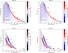 |
Fig. A.1 Data distributions of the profiles of the spectral lines J = 5–4 and J = 2–1 of HCN and HNC parametrised with the variables (I, Δv). The upper and lower rows show the data distributions of J = 5–4 and J = 2–1, respectively, for HCN (left panels) and HNC (right panels). The HNC/HCN ratio and the source’s size are fixed to 0.8 and 5 arcsec, respectively. As the data are distributed by branches of points, corresponding to the steps of ΔVsys, only those with ΔVsys = 1, 5, 10 and 15 km/s are showcased for the sake of clarity. |
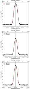 |
Fig. A.2 Spectra of the HCN (5–4), HNC (3–2), and HNC (4–3) transitions towards Orion KL (Vlsr ≈ 9.4 km s−1) combined with LTE-MCMC models representing the conditions of a hot core with an excitation temperature of 90 K and N(HNC)/N(HCN) = 0.8, calculated with a fixed value of N(HCN) ≃ 1 × 1015 cm−2. |
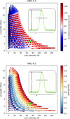 |
Fig. A.3 Data distribution of the profiles of the simulated spectral line J = 4–3 of HNC for the grid of physical parameters values. The top display shows the temperature mapping of the data while the bottom one shows the abundance ratio mapping. Both panels depict the HNC J = 4–3 line transition, from which the line intensity and linewidth, along with their associated error bars, are obtained for the semi-empirical data of Orion KL. These values are indicated by a green dot in each panel. |
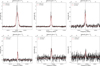 |
Fig. A.4 APEX-detected spectral lines of HCN and HNC isotopologues towards R CrA IRS 7B (black histogram), with corresponding LTEMCMC models shown as solid red lines. The HCN and HNC J = 3–2 transitions, exhibiting excitation temperatures (Texc) of 26(5) K and 27(5) K, respectively, and a column density ratio N(HNC)/N(HCN) ≈ 0.30. The H13CN and HN13C J = 3–2 transitions, with Texc of 11(3) K and 12(2) K, respectively, and N(HN13C)/N(H13CN) ≈ 0.38. The HC15N and H15NC J = 3–2 transitions, with Texc of 11(4) K and 14(2) K, respectively, and N(HN15C)/N(HC15N) ≈ 0.39. |
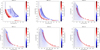 |
Fig. A.5 Data distributions derived from the variables (I, Δv), obtained from the HCN and HNC spectral transitions J = 1–0, J = 3–2, and J = 4–3, under the assumption of hypothetical HNC/HCN abundance ratios and source sizes of 0.8 and 5 arcsec, respectively. |
References
- Baiano, C., Lupi, J., Barone, V., & Tasinato, N., 2022, J. Chem. Theory Comput., 18, 3111 [CrossRef] [Google Scholar]
- Behrens, E., Mangum, J. G., Holdship, J., et al. 2022, ApJ, 939, 119 [NASA ADS] [CrossRef] [Google Scholar]
- Binney, J., & Tremaine, S., 2008, Galactic Dynamics, 2nd revised edn. (Princeton University Press) [Google Scholar]
- Blake, G. A., Sutton, E. C., Masson, C. R., & Phillips, T. G., 1987, ApJ, 315, 621 [Google Scholar]
- Breiman, L. 2001, Mach. Learn., 45, 5 [Google Scholar]
- Bron, E., Roueff, E., Gerin, M., et al. 2021, A&A, 645, A28 [NASA ADS] [CrossRef] [EDP Sciences] [Google Scholar]
- Brooks, D. G., Carroll, S. S., & Verdini, W. A., 1988, Am. Statist., 42, 187 [Google Scholar]
- Brouillet, N., Despois, D., Lu, X. H., et al. 2015, A&A, 576, A129 [NASA ADS] [CrossRef] [EDP Sciences] [Google Scholar]
- Buchner, J., & Fotopoulou, S., 2024, Nat. Rev. Phys., 6, 535 [Google Scholar]
- Burman, P., 1989, Biometrika, 76, 503 [Google Scholar]
- Carvajal, M., Margulès, L., Tercero, B., et al. 2009, A&A, 500, 1109 [CrossRef] [EDP Sciences] [Google Scholar]
- Carvajal, M., Kleiner, I., & Demaison, J., 2010, ApJS, 190, 315 [NASA ADS] [CrossRef] [Google Scholar]
- Carvajal, M., Favre, C., Kleiner, I., et al. 2019, A&A, 627, A65 [NASA ADS] [CrossRef] [EDP Sciences] [Google Scholar]
- Carvajal, M., Favre, C., Kleiner, I., et al. 2024, A&A, 685, C1 [NASA ADS] [CrossRef] [EDP Sciences] [Google Scholar]
- Cernicharo, J., Tercero, B., Marcelino, N., Agúndez, M., & de Vicente, P., 2023, A&A, 674, L4 [NASA ADS] [CrossRef] [EDP Sciences] [Google Scholar]
- Chen, T., & Guestrin, C., 2016, in KDD ‘16: Proceedings of the 22nd ACM SIGKDD International Conference on Knowledge Discovery and Data Mining, 785 [CrossRef] [Google Scholar]
- Comito, C., Schilke, P., Phillips, T. G., et al. 2005, ApJS, 156, 127 [NASA ADS] [CrossRef] [Google Scholar]
- Delli Veneri, M., Tychoniec, Ł., Guglielmetti, F., Longo, G., & Villard, E. 2023, MNRAS, 518, 3407 [Google Scholar]
- de Vicente, P., Martín-Pintado, J., Neri, R., & Rodríguez-Franco, A., 2002, ApJ, 574, L163 [NASA ADS] [CrossRef] [Google Scholar]
- Draine, B. T., 2011, Physics of the Interstellar and Intergalactic Medium (Princeton University Press) [Google Scholar]
- Dumke, M., & Mac-Auliffe, F., 2010, SPIE Conf. Ser., 7737, 77371J [Google Scholar]
- Dumouchel, F., Faure, A., & Lique, F., 2010, MNRAS, 406, 2488 [NASA ADS] [CrossRef] [Google Scholar]
- Dumouchel, F., Kłos, J., & Lique, F., 2011, Phys. Chem. Chem. Phys. (Incorp. Faraday Trans.), 13, 8204 [NASA ADS] [CrossRef] [Google Scholar]
- Einig, L., Pety, Jérôme, Roueff, Antoine, et al. 2023, A&A, 677, A158 [NASA ADS] [CrossRef] [EDP Sciences] [Google Scholar]
- Einig, L., Palud, P., Roueff, A., et al. 2024, A&A, 691, A109 [NASA ADS] [CrossRef] [EDP Sciences] [Google Scholar]
- Endres, C. P., Schlemmer, S., Schilke, P., Stutzki, J., & Müller, H. S. P., 2016, J. Mol. Spectrosc., 327, 95 [NASA ADS] [CrossRef] [Google Scholar]
- Esplin, T. L., & Luhman, K. L., 2022, AJ, 163, 64 [NASA ADS] [CrossRef] [Google Scholar]
- Foreman-Mackey, D., Hogg, D. W., Lang, D., & Goodman, J., 2013, PASP, 125, 306 [Google Scholar]
- Fukushima, K., 1969, IEEE Trans. Syst. Sci. Cybernet., 5, 322 [Google Scholar]
- Galli, P. A. B., Bouy, H., Olivares, J., et al. 2020, A&A, 634, A98 [NASA ADS] [CrossRef] [EDP Sciences] [Google Scholar]
- Galliano, F., Madden, S. C., Jones, A. P., et al. 2003, A&A, 407, 159 [NASA ADS] [CrossRef] [EDP Sciences] [Google Scholar]
- Galliano, F., Nersesian, A., Bianchi, S., et al. 2021, A&A, 649, A18 [EDP Sciences] [Google Scholar]
- Girosi, F., Jones, M., & Poggio, T., 1995, Neural Computat., 7, 219 [Google Scholar]
- Goldsmith, P. F., & Langer, W. D., 1999, ApJ, 517, 209 [Google Scholar]
- Graninger, D. M., Herbst, E., Öberg, K. I., & Vasyunin, A. I., 2014, ApJ, 787, 74 [Google Scholar]
- Gratier, P., Majumdar, L., Ohishi, M., et al. 2016, ApJS, 225, 25 [Google Scholar]
- Gratier, P., Pety, J., Bron, E., et al. 2021, A&A, 645, A27 [CrossRef] [EDP Sciences] [Google Scholar]
- Guerra-Varas, N., Merello, M., Bronfman, L., et al. 2023, A&A, 677, A148 [NASA ADS] [CrossRef] [EDP Sciences] [Google Scholar]
- Güsten, R., Nyman, L. Å., Schilke, P., et al. 2006, A&A, 454, L13 [NASA ADS] [CrossRef] [EDP Sciences] [Google Scholar]
- Hacar, A., Bosman, A. D., & van Dishoeck, E. F., 2020, A&A, 635, A4 [NASA ADS] [CrossRef] [EDP Sciences] [Google Scholar]
- Haykin, S., 1999, Neural Networks: A Comprehensive Foundation (Prentice Hall Ed.) [Google Scholar]
- Hernández Vera, M., Lique, F., Dumouchel, F., Hily-Blant, P., & Faure, A., 2017, MNRAS, 468, 1084 [Google Scholar]
- Hervías-Caimapo, C., Merello, M., Bronfman, L., et al. 2019, ApJ, 872, 200 [Google Scholar]
- Hirota, T., Yamamoto, S., Mikami, H., & Ohishi, M., 1998, ApJ, 503, 717 [Google Scholar]
- Ho, T. K., 1995, in Proceedings of the Third International Conference on Document Analysis and Recognition, 1, ICDAR ’95 (M: IEEE Computer Society), 278 [Google Scholar]
- Holdship, J., Mangum, J. G., Viti, S., et al. 2022, ApJ, 931, 89 [NASA ADS] [CrossRef] [Google Scholar]
- Hornik, K., Stinchcombe, M., & White, H., 1989, Neural Networks, 2, 359 [CrossRef] [Google Scholar]
- Householder, A. S., 1941, Bull. Math. Biophys., 3, 63 [Google Scholar]
- Imanishi, M., Nakanishi, K., & Izumi, T., 2017, ApJ, 849, 29 [NASA ADS] [CrossRef] [Google Scholar]
- Jain, A., Duin, R., & Mao, J., 2000, IEEE Trans. Pattern Anal. Mach. Intell., 22, 4 [CrossRef] [Google Scholar]
- Jin, M., Lee, J.-E., & Kim, K.-T., 2015, ApJS, 219, 2 [Google Scholar]
- Joblin, C., Bron, E., Pinto, C., et al. 2018, A&A, 615, A129 [NASA ADS] [CrossRef] [EDP Sciences] [Google Scholar]
- Jørgensen, J. K., Belloche, A., & Garrod, R. T., 2020, ARA&A, 58, 727 [Google Scholar]
- Jung, S. H., & Choe, J. C., 2013, Astrobiology, 13, 465 [Google Scholar]
- Kama, M., López-Sepulcre, A., Dominik, C., et al. 2013, A&A, 556, A57 [NASA ADS] [CrossRef] [EDP Sciences] [Google Scholar]
- Khalouf-Rivera, J., Carvajal, M., Santos, L. F., & Pérez-Bernal, F., 2019, J. Phys. Chem. A, 123, 9544 [Google Scholar]
- Kingma, D. P., & Ba, J., 2014, arXiv e-prints [arXiv:1412.6980] [Google Scholar]
- Kingma, D. P., & Ba, J., 2015, in 3rd International Conference on Learning Representations, ICLR 2015, San Diego, CA, USA, May 7–9, 2015, Conference Track Proceedings, eds. Y. Bengio & Y. LeCun [Google Scholar]
- Kounkel, M., Hartmann, L., Loinard, L., et al. 2017, ApJ, 834, 142 [Google Scholar]
- Lebouteiller, V., & Ramambason, L., 2022, A&A, 667, A34 [NASA ADS] [CrossRef] [EDP Sciences] [Google Scholar]
- Lee, K. L. K., Patterson, J., Burkhardt, A. M., et al. 2021, ApJ, 917, L6 [NASA ADS] [CrossRef] [Google Scholar]
- Lefloch, B., Bachiller, R., Ceccarelli, C., et al. 2018, MNRAS, 477, 4792 [Google Scholar]
- Li, D., Tang, X., Henkel, C., et al. 2020, ApJ, 901, 62 [NASA ADS] [CrossRef] [Google Scholar]
- Long, F., Bosman, Arthur D., Cazzoletti, Paolo, et al. 2021, A&A, 647, A118 [NASA ADS] [CrossRef] [EDP Sciences] [Google Scholar]
- Mangum, J. G., & Shirley, Y. L., 2015, PASP, 127, 266 [Google Scholar]
- Martin, C. H., Peng, T. S., & Mahoney, M. W., 2021, Nat. Commun., 12, 4122 [Google Scholar]
- McGuire, B. A., Burkhardt, A. M., Loomis, R. A., et al. 2020, ApJ, 900, L10 [Google Scholar]
- McGuire, B., Loomis, R., Burkhardt, A., et al. 2021, Science, 371, 1265 [NASA ADS] [CrossRef] [Google Scholar]
- Meijerink, R., Spaans, M., Loenen, A. F., & van der Werf, P. P., 2011, A&A, 525, A119 [NASA ADS] [CrossRef] [EDP Sciences] [Google Scholar]
- Mendes, M. B., Buhr, H., Berg, M. H., et al. 2012, ApJ, 746, L8 [NASA ADS] [CrossRef] [Google Scholar]
- Mendoza, E., Lefloch, B., Ceccarelli, C., et al. 2018, MNRAS, 475, 5501 [NASA ADS] [CrossRef] [Google Scholar]
- Mendoza, E., Carvajal, M., Merello, M., Bronfman, L., & Boechat-Roberty, H. M., 2023, ApJ, 953, 77 [Google Scholar]
- Mesa, D., Bonnefoy, M., Gratton, R., et al. 2019, A&A, 624, A4 [NASA ADS] [CrossRef] [EDP Sciences] [Google Scholar]
- Mika, J., & Devika, T., 2024, A&A, 685, A164 [NASA ADS] [CrossRef] [EDP Sciences] [Google Scholar]
- Milam, S. N., Savage, C., Brewster, M. A., Ziurys, L. M., & Wyckoff, S., 2005, ApJ, 634, 1126 [Google Scholar]
- Nickerson, S., Rangwala, N., Colgan, S. W. J., et al. 2021, ApJ, 907, 51 [NASA ADS] [CrossRef] [Google Scholar]
- Nyheim, B., Riemer-Sørensen, S., Parra, R., & Cicone, C., 2024, arXiv e-prints [arXiv:2402.08589] [Google Scholar]
- Paumard, T., Ciurlo, A., Morris, M. R., Do, T., & Ghez, A. M., 2022, A&A, 664, A97 [NASA ADS] [CrossRef] [EDP Sciences] [Google Scholar]
- Pazukhin, A. G., Zinchenko, I. I., Trofimova, E. A., Henkel, C., & Semenov, D. A., 2023, MNRAS, 526, 3673 [NASA ADS] [CrossRef] [Google Scholar]
- Pedregosa, F., Varoquaux, G., Gramfort, A., et al. 2011, J. Mach. Learn. Res., 12, 2825 [Google Scholar]
- Pérez-Beaupuits, J. P., Aalto, S., & Gerebro, H., 2007, A&A, 476, 177 [NASA ADS] [CrossRef] [EDP Sciences] [Google Scholar]
- Perotti, G., Jørgensen, J. K., Rocha, W. R. M., et al. 2023, A&A, 678, A78 [NASA ADS] [CrossRef] [EDP Sciences] [Google Scholar]
- Pety, J., Guzmán, V. V., Orkisz, J. H., et al. 2017, A&A, 599, A98 [NASA ADS] [CrossRef] [EDP Sciences] [Google Scholar]
- Pickett, H. M., Poynter, R. L., Cohen, E. A., et al. 1998, J. Quant. Spec. Radiat. Transf., 60, 883 [Google Scholar]
- Priestley, M., O’donnell, F., & Simperl, E., 2023, A&A, 15 [Google Scholar]
- Ramambason, L., Lebouteiller, V., Bik, A., et al. 2022, A&A, 667, A35 [NASA ADS] [CrossRef] [EDP Sciences] [Google Scholar]
- Roueff, E., & Lique, F., 2013, Chem. Rev., 113, 8906 [Google Scholar]
- Roueff, A., Gerin, Maryvonne, Gratier, Pierre, et al. 2021, A&A, 645, A26 [NASA ADS] [CrossRef] [EDP Sciences] [Google Scholar]
- Roueff, A., Pety, J., Gerin, M., et al. 2024, A&A, 686, A255 [NASA ADS] [CrossRef] [EDP Sciences] [Google Scholar]
- Rumelhart, D. E., Hinton, G. E., & Williams, R. J., 1986, Nature, 323, 533 [Google Scholar]
- Schapire, R. E., 2003, The Boosting Approach to Machine Learning: An Overview, eds. D. D. Denison, M. H. Hansen, C. C. Holmes, B. Mallick, & B. Yu (New York, NY: Springer New York), 149 [Google Scholar]
- Schilke, P., Walmsley, C. M., Pineau Des Forets, G., et al. 1992, A&A, 256, 595 [Google Scholar]
- Schilke, P., Groesbeck, T. D., Blake, G. A., Phillips, & T. G. 1997, ApJS, 108, 301 [NASA ADS] [CrossRef] [Google Scholar]
- Schöier, F. L., Jørgensen, J. K., Pontoppidan, K. M., & Lundgren, A. A., 2006, A&A, 454, L67 [NASA ADS] [CrossRef] [EDP Sciences] [Google Scholar]
- Schöier, F. L., Bast, J., Olofsson, H., & Lindqvist, M., 2007, A&A, 473, 871 [NASA ADS] [CrossRef] [EDP Sciences] [Google Scholar]
- Shaw, A. M., 2006, Astrochemistry: From astronomy to Astrobiology (Wiley Ltd.) [Google Scholar]
- Shimajiri, Y., Sakai, T., Kitamura, Y., et al. 2015, ApJS, 221, 31 [CrossRef] [Google Scholar]
- Shirley, Y. L., 2015, PASP, 127, 299 [Google Scholar]
- Sola, J., & Sevilla, J., 1997, Nucl. Sci. IEEE Trans., 44, 1464 [Google Scholar]
- Stanke, T., Arce, H. G., Bally, J., et al. 2022, A&A, 658, A178 [NASA ADS] [CrossRef] [EDP Sciences] [Google Scholar]
- Tachikawa, H., Iyama, T., & Fukuzumi, T., 2003, A&A, 397, 1 [Google Scholar]
- Taniguchi, K., Rayalacheruvu, P., Yonetsu, T., et al. 2024, ApJ, 963, 12 [Google Scholar]
- van der Tak, F., 2011, in IAU Symposium, 280, The Molecular Universe, eds. J. Cernicharo & R. Bachiller, 449 [Google Scholar]
- van der Tak, F., Black, J. H., Schöier, F. L., Jansen, D. J., & van Dishoeck, E. F., 2007, A&A, 468, 627 [NASA ADS] [CrossRef] [EDP Sciences] [Google Scholar]
- van der Tak, F., Lique, F., Faure, A., Black, J.H., & van Dishoeck, E. F., 2020, Atoms, 8, 15 [NASA ADS] [CrossRef] [Google Scholar]
- Vassilev, V., Meledin, D., Lapkin, I., et al. 2008, A&A, 490, 1157 [NASA ADS] [CrossRef] [EDP Sciences] [Google Scholar]
- Vastel, C., Bottinelli, S., Caux, E., Glorian, J. M., & Boiziot, M., 2015, in SF2A2015: Proceedings of the Annual meeting of the French Society of Astronomy and Astrophysics, eds. F. Martins, S. Boissier, V. Buat, L. Cambrésy, & P. Petit, 313 [Google Scholar]
- Vera, M. H., Kalugina, Y., Denis-Alpizar, O., Stoecklin, T., & Lique, F., 2014, J. Chem. Phys., 140, 224302 [CrossRef] [Google Scholar]
- Wampfler, S. F., Jørgensen, J. K., Bizzarro, M., & Bisschop, S. E., 2014, A&A, 572, A24 [NASA ADS] [CrossRef] [EDP Sciences] [Google Scholar]
- Watanabe, Y., Sakai, N., Lindberg, J. E., et al. 2012, ApJ, 745, 126 [NASA ADS] [CrossRef] [Google Scholar]
- Wilson, T. L., & Rood, R., 1994, Annu. Rev. Astron. Astrophys., 32, 191 [Google Scholar]
- Wilson, T. L., Rohlfs, K., & Hüttemeister, S., 2013, Tools of Radio Astronomy (Springer) [Google Scholar]
- Wright, M. C. H., & Plambeck, R. L., 2017, ApJ, 843, 83 [Google Scholar]
- Xu, Q.-S., & Liang, Y.-Z. 2001, Chemom. Intell. Lab. Syst., 56, 1 [Google Scholar]
- Yamashita, T., Miyamura, N., & Kawai, S., 2023, J. Chem. Phys., 159, 124116 [Google Scholar]
- Yang, Y.-L., Green, J. D., II, NJE, et al. 2018, ApJ, 860, 174 [NASA ADS] [CrossRef] [Google Scholar]
- Zamir, A., & Stein, T., 2022, J. Chem. Phys., 156, 054307 [Google Scholar]
Splatalogue, CDMS, JPL Molecular Spectroscopy, NIST Recommended Rest Frequencies
This property applies for arbitrary layer width.
In ML, the target variables are the output variables.
The convex hull defined by a set of vector points in any dimension is the smallest convex set that contains them. It is a geometrical construction (not the only one) used to determine whether a point interpolates or not the training dataset domain (Brooks et al. 1988).
All Tables
Spectroscopic parameters of the observed lines towards R CrA IRS 7B, including Gaussian-integrated areas and LTE-MCMC derived results for HCN and HNC and their 13C and 15N isotopologues.
Performance metrics and temperature predictions for Orion KL hot core from the RF, XGB, and MLP models.
Performance metrics and ratios predictions of HNC/HCN for the Orion KL hot core from the RF, XGB, and MLP models.
Performance metrics and temperature predictions for the cold source R CrA IRS 7B from the RF, XGB, and MLP models.
Performance metrics and ratios predictions of HNC/HCN for the cold source R CrA IRS 7B from the RF, XGB, and MLP models.
All Figures
|
Fig. 1 Schematic of the workflow for training and evaluating ML models to predict excitation temperatures and isomeric ratios from HCN and HNC spectra. Data preparation integrates models and observations to build a dataset. Gaussian fit parameters are used to generate a data cloud of line intensity vs. width, gradient-tagged by temperatures and ratios. Training and testing stages utilise three algorithms, with results benchmarked against radiative transfer models and validated using observational prototype data. |
| In the text | |
|
Fig. A.1 Data distributions of the profiles of the spectral lines J = 5–4 and J = 2–1 of HCN and HNC parametrised with the variables (I, Δv). The upper and lower rows show the data distributions of J = 5–4 and J = 2–1, respectively, for HCN (left panels) and HNC (right panels). The HNC/HCN ratio and the source’s size are fixed to 0.8 and 5 arcsec, respectively. As the data are distributed by branches of points, corresponding to the steps of ΔVsys, only those with ΔVsys = 1, 5, 10 and 15 km/s are showcased for the sake of clarity. |
| In the text | |
|
Fig. A.2 Spectra of the HCN (5–4), HNC (3–2), and HNC (4–3) transitions towards Orion KL (Vlsr ≈ 9.4 km s−1) combined with LTE-MCMC models representing the conditions of a hot core with an excitation temperature of 90 K and N(HNC)/N(HCN) = 0.8, calculated with a fixed value of N(HCN) ≃ 1 × 1015 cm−2. |
| In the text | |
|
Fig. A.3 Data distribution of the profiles of the simulated spectral line J = 4–3 of HNC for the grid of physical parameters values. The top display shows the temperature mapping of the data while the bottom one shows the abundance ratio mapping. Both panels depict the HNC J = 4–3 line transition, from which the line intensity and linewidth, along with their associated error bars, are obtained for the semi-empirical data of Orion KL. These values are indicated by a green dot in each panel. |
| In the text | |
|
Fig. A.4 APEX-detected spectral lines of HCN and HNC isotopologues towards R CrA IRS 7B (black histogram), with corresponding LTEMCMC models shown as solid red lines. The HCN and HNC J = 3–2 transitions, exhibiting excitation temperatures (Texc) of 26(5) K and 27(5) K, respectively, and a column density ratio N(HNC)/N(HCN) ≈ 0.30. The H13CN and HN13C J = 3–2 transitions, with Texc of 11(3) K and 12(2) K, respectively, and N(HN13C)/N(H13CN) ≈ 0.38. The HC15N and H15NC J = 3–2 transitions, with Texc of 11(4) K and 14(2) K, respectively, and N(HN15C)/N(HC15N) ≈ 0.39. |
| In the text | |
|
Fig. A.5 Data distributions derived from the variables (I, Δv), obtained from the HCN and HNC spectral transitions J = 1–0, J = 3–2, and J = 4–3, under the assumption of hypothetical HNC/HCN abundance ratios and source sizes of 0.8 and 5 arcsec, respectively. |
| In the text | |
Current usage metrics show cumulative count of Article Views (full-text article views including HTML views, PDF and ePub downloads, according to the available data) and Abstracts Views on Vision4Press platform.
Data correspond to usage on the plateform after 2015. The current usage metrics is available 48-96 hours after online publication and is updated daily on week days.
Initial download of the metrics may take a while.