| Issue |
A&A
Volume 698, June 2025
|
|
|---|---|---|
| Article Number | A159 | |
| Number of page(s) | 17 | |
| Section | The Sun and the Heliosphere | |
| DOI | https://doi.org/10.1051/0004-6361/202451830 | |
| Published online | 11 June 2025 | |
What does solar chromospheric activity look like under different inclination angles?
1
Department of Solar Physics and Space Weather, Royal Observatory of Belgium (ROB), Av. Circulaire 3, 1180 Uccle, Belgium
2
Space Sciences, Technologies and Astrophysics Research (STAR) Institute, Université de Liège, Allée du 6 Août, 19c, Bât B5c, 4000 Liège, Belgium
3
Institut d’Astronomie et d’Astrophysique (IAA), Université Libre de Bruxelles, CP 226, Boulevard du Triomphe, 1050 Bruxelles, Belgium
⋆ Corresponding author: This email address is being protected from spambots. You need JavaScript enabled to view it.
Received:
7
August
2024
Accepted:
21
March
2025
Abstract
Context. Chromospheric observations in the Ca II lines are essential for studying the magnetic activity of stars. In the case of the Sun, the chromospheric plages, the main contributors to the Ca II K emission, are distributed between midlatitude and the equator and never close to the poles. Therefore, we suspect that the inclination angle of the solar rotation axis has an impact on the observable chromospheric emission. Until now, the effect of such an inclination on chromospheric emission has not been extensively studied through direct solar observations.
Aims. We reproduce solar images from any inclination to study the effect of the inclination axis on the solar variability by using direct observations of the Sun in the Ca II K line. In the context of the solar-stellar connection, while the Sun is observed from Earth from its near-equator point of view, and the other stars are observed most of the time under unknown inclinations, our results can improve our understanding of the magnetic activity of other solar-type stars.
Methods. More than 2700 days of observations since the beginning of the Ca II K observations with the Uccle Solar Equatorial Table (USET), in July 2012, were used in our analysis. For each observation day, we produced synoptic maps to map the entire solar surface during a full solar rotation. Then, by choosing a given inclination, we generated solar-disk views, representing the segmented brightest structures of the chromosphere (plages and enhanced network) as seen under this inclination. The area fractions were extracted from the masks for each inclination and we compared the evolution of those time series to quantify the impact of the inclination angle.
Results. We find a variation of the area fraction between an equator-on view and a pole-on view. Our results show an important impact of the viewing angle on the detection of modulation due to the solar rotation. With the dense temporal sampling of USET data, the solar rotation is detectable up to an inclination of about |i| = 70° and the solar cycle modulation is clearly detected for all inclinations, though with a reduced amplitude in polar views. When applying a sparse temporal sampling typical for time series of solar-like stars, the rotational modulation is no longer detected, whatever the inclination, due entirely to the undersampling. On the other hand, we find that the activity cycle modulation remains detectable, even for pole-on inclinations, as long as the sampling contains at least 20 observations per year and the cycle amplitude reaches at least 30% of the solar cycle amplitude.
Conclusions. The inclination of the rotation axis of stars relative to our line of sight is unknown most of the time. Based on solar observations, we show that the impact of this inclination is important for the detection of the rotation period but negligible for the detection of the activity cycle period. For other stars, the time series usually have more complicated and scarcer samplings due to restricted target visibility, and this leads to a decrease in the signal of the chromospheric activity cycle. However, our results suggest that the inclination is unlikely to be the primary factor contributing to the relative scarcity of well-established cycles.
Key words: Sun: activity / Sun: chromosphere / Sun: faculae / plages / stars: activity / stars: solar-type
© The Authors 2025
 Open Access article, published by EDP Sciences, under the terms of the Creative Commons Attribution License (https://creativecommons.org/licenses/by/4.0), which permits unrestricted use, distribution, and reproduction in any medium, provided the original work is properly cited.
This article is published in open access under the Subscribe to Open model. This email address is being protected from spambots. You need JavaScript enabled to view it. to support open access publication.
1. Introduction
The chromospheric activity of a large number of stars is monitored in the Ca II K and H lines (Radick et al. 2018; Boro Saikia et al. 2018; Mittag et al. 2023). Over the past 60 years, significant progress has been made in the study of cool stellar chromospheres. It started in 1966, with the Mount Wilson HK project (Wilson 1978) recording chromospheric measurements of approximately 2000 Sun-like stars. Understanding how the Sun compares to Sun-like stars in terms of variability and magnetic activity cycles can provide profound insights into the mechanisms driving stellar magnetic activity. The Mount Wilson HK project led to the creation of the Mount Wilson S-index, defined as the ratio of the total flux in the Ca II K and H line cores to the total flux in two pseudocontinuum regions located near the K and H lines. This index is widely used to study the magnetic activity of stars. In particular, the stellar cycle and rotation can be calculated based on the detection of temporal modulations in the time series of the S-index (Hempelmann et al. 2016). For instance, the Mount Wilson monitoring program demonstrated that the Sun is not unique in exhibiting periodic activity cycles (Baliunas et al. 1998): such behavior is common among solar-like stars (60% of Wilson’s sample stars). However, some studies have demonstrated that most Sun-like stars (with age, mass, temperature, and chromospheric activity similar to the Sun) exhibit different photometric variability on the activity cycle timescale than the Sun (Lockwood & Skiff 1990; Lockwood et al. 2007; Reinhold et al. 2020). The impact of the viewing angle on the solar irradiance variability was first proposed by Schatten (1993). Indeed, the magnetic structures are distributed between the equator and midlatitudes, and the position of the observer relative to the rotation axis affects their brightness contrasts. While stars are usually observed without information on their inclinations, it is crucial to quantitatively evaluate this dependence to understand how solar variability is comparable to other Sun-like stars. In addition it can impact the detectability of exoplanets and the determination of their mass (Meunier et al. 2023).
The rotation periods of stars have been successfully estimated from S-index time series, but no correction for the effect of inclination on the observed level of variability was applied (Vaughan et al. 1981; Noyes et al. 1984; Baliunas et al. 1985; Wright et al. 2004). More recently, Radick et al. (2018) studied the variation of the chromospheric emission of the Sun and other Sun-like stars, but they also did not apply a correction for the effect of inclination. The impact of the viewing angle on the observable magnetic activity of the Sun has been studied mainly on the basis of synthetic images of the Sun obtained with rather simplified models and numerical simulations (Schatten 1993; Knaack et al. 2001; Shapiro et al. 2014; Borgniet et al. 2015; Meunier et al. 2019, 2024; Nèmec et al. 2020; Sowmya et al. 2021). For example, Shapiro et al. (2014), Knaack et al. (2001), and Sowmya et al. (2021) analyzed the influence of the inclination on solar irradiance and chromospheric activity by using physics-based models to calculate relative flux variations. Borgniet et al. (2015) and Meunier et al. (2019) present similar studies, but using time series of radial velocity, chromospheric emission, and photometry to analyze the effects of activity (via spots, faculae, and inhibition of convective blueshift) on exoplanet detectability. Those studies show, through simulations of different inclinations, that the inclination of the stellar rotation axis has a strong impact on those time series. Here we propose to study this impact on the determination of the temporal modulations through real solar observations in the Ca II K line.
Ground-based solar observations only allow us to see the surface of the near side of the Sun. However, based on images recorded during a full solar rotation, we can map the entire solar surface into a synoptic map. Then, by an appropriate projection, we can generate images of the Sun for various viewing angles. Finally, we can build time series for different inclinations and study the impact on the detection of modulations. More specifically, we can consider the effect on the time series of the plages and enhanced network area fraction in the Ca II K line.
In fact, it has been shown that those structures are the main cause of the modulation in the Ca II K emission, and that their area fraction is a good proxy for the S-index. Using Ca II K images with USET and the S-index collected from TIGRE (Telescopio Internacional de Guanajuato Robotico Espectroscopico), Vanden Broeck et al. (2024) compare the area fraction of plages and enhanced network with the S-index, based on data obtained over the same time interval and for observations made on the same dates. As seen in Fig. 1, they find a linear correlation between the indices, described by the following equation:
 (1)
(1)
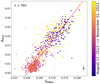 |
Fig. 1. Correlation between daily values of the solar S-index from TIGRE (in the Mount Wilson scale) and the USET area fraction of plages and enhanced network, APEN. The parameter n represents the number of data, and the chronological order is color coded. The first and last dates of the data are given next to the color bar. Additionally, a linear fit to the data was performed (solid red line). A mean error bar is displayed in the bottom right corner to give an idea of the uncertainties on the data. Image taken from Vanden Broeck et al. (2024). |
where APEN is the area fraction of the plages and enhanced network from USET images, and SMWO the solar S-index from TIGRE in the Mount Wilson scale. Since a well-defined linear transformation is found to convert the S-index from TIGRE to the Mount Wilson scale (Mittag et al. 2016), the area fraction of plages and enhanced network offers a reliable diagnostic of chromospheric activity. This area fraction can then be used to generalize the results obtained for the Sun to the population of Sun-like stars.
Section 2 briefly describes the instrument and data used for our analysis. In Section 3, we explain the method of data processing: the segmentation of the chromospheric structures, the creation of the synoptic maps, and the production of the solar-disk views under different inclination angles. Our results on the detection of the temporal modulation for various inclinations are presented in Section 4. Finally, we summarize and discuss our results in Section 5.
2. Dataset
In this study, we used the synoptic images acquired by the USET station from the Royal Observatory of Belgium (ROB), located in Uccle, south of Brussels (Bechet & Clette 2002). Synoptic images are appropriate for this study as the full-disk images cover the whole surface of the Sun, which is needed to map the entire solar surface. In particular, we considered the full-disk daily images in the Ca II K line. The dataset covers a long time period, from July 11, 2012 to November 28, 2023, thus spanning 11.38 years, which is required to search for long temporal modulations. After performing an automatic quality selection to keep the best image recorded per day (Vanden Broeck et al. 2024), the resulting series consisted of 2725 images, covering more than 70% of the analyzed period.
In addition, the station carries three other solar telescopes (White-Light, 656.3 nm H-alpha, and sunspot drawings) to simultaneously monitor the photosphere and the chromosphere. The averaged total number of observation days is 260 per year. The gaps are essentially due to bad weather conditions.
The optical setup consists of a refractor of 925 mm focal length and 132 mm aperture. The filter is thermo-regulated and its central wavelength is λ = 3933.67 Å, with a bandwidth of 2.7Å. The images are acquired with a 2048 × 2048 CCD (charge-coupled device) with a dynamic range of 12 bits. The instrumental setup has been the same since 2012, except for the introduction of an additional neutral filter on July 10, 2013. The acquisition cadence can go up to 4 frames per second in case of transient events to record, and the daily synoptic cadence is 15 minutes.
3. Data processing
After correcting the raw USET Ca II K images for instrumental and atmospheric effects, we segmented the brightest chromospheric features to generate binary masks. Then, using successive daily disk masks, we assembled synoptic maps, each covering a full Carrington rotation, thus mapping the whole solar surface. We were then able to apply a spherical projection to those synthetic maps to create solar-disk views reproducing the projected area of bright chromospheric structures as seen under different inclinations of the rotation axis relative to the line of sight. Finally, by summing those apparent areas over the full disk for each date, we created a time series of the total area fraction that spanned the duration of the USET dataset.
In the next sections, we define the inclination as the angle between the solar equator and the observer’s line of sight. The equator-on view refers to an inclination i = 0°, while the pole-on view corresponds to an inclination i = 90° for the north pole-on view and i = −90° for the south pole-on view.
3.1. Chromospheric structures segmentation
The solar chromosphere exhibits various structures that differ in size and brightness. In this study, we segmented the brightest structures, namely the plages, which are the chromospheric counterparts of the faculae, and the enhanced network, considered as small regions of decaying plages (Singh et al. 2023). More details on this segmentation method can be found in Vanden Broeck et al. (2024), and an example of this process is shown in Fig. 2.
 |
Fig. 2. Example of the segmentation process. Left: Recentered raw image from October 29, 2013. Right: Result of the segmentation. |
3.2. Synoptic segmented map construction
To map the entire solar surface, a projection is needed to convert spherical coordinates (latitude and longitude) into a flat representation. For this, we used the Plate Carrée (CAR) projection where the meridians and the parallels are equally spaced, forming a grid of squares from east to west and from north to south. With this projection, it is particularly easy to associate the heliographic coordinates of a structure on the Sun with its position in pixels on the map (Calabretta & Greisen 2002). Fig. 3 shows an example of the CAR projection of a solar image. The white part of the image is due to the fact that the rotation axis of the Sun is tilted with respect to the ecliptic. This tilt goes from −7.25° to 7.25°. Therefore, except when this inclination is equal to 0°, there is always a small hidden area around either the north or the south pole. Those parts of the images are filled with zero values.
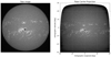 |
Fig. 3. Example of a CAR projection. Left: Raw solar image. Right: Corresponding image after the projection. |
A synoptic map is made of consecutive strips from successive solar images that span a whole solar rotation. In each image, the strip is centered on the central meridian and its pixel size corresponds to a time interval depending on the observing time of the previous and the following available images. This process is applied for each day of the dataset. Finally, by doing a calculation for the boundary conditions to build a map of 180° before and 180° after a given day, we get a synoptic map representing the entire surface of the Sun around this given date (see Fig. 4).
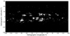 |
Fig. 4. Example of a segmented synoptic map built around July 7, 2014, illustrating the distribution of the plages and enhanced network during a full solar rotation. The x-axis represents the number of degrees of longitude from the Carrington longitude on July 7, 2014 (center of image). |
3.3. Reconstructed solar-disk views for different inclinations
For each observed date in the original USET series, using the corresponding whole-Sun segmented synoptic map, we created solar-disk views at different inclinations by using an orthographic projection with various centers. In particular, we specified the central latitude and longitude in the orthographic function from the Cartopy library, designed for cartographic projection and geospatial data visualization (Met Office 2010–2015). The generation of solar-disk views is illustrated in Fig. 5 for inclinations, i, of 0°, 30°, 60°, and 90° (from the equator-on view to the north pole-on view). Appendix A provides the generated solar-disk views for all the inclinations from the north pole-on view to the south pole-on view. The gray areas on the synoptic maps in Fig. 5 represent the far side of the Sun. The chromospheric plages are distributed up to 50° of latitude relative to the equator (Devi et al. 2021). Therefore, as we move to a pole-on observation, those structures will be distributed closer to the limbs, which makes them appear smaller.
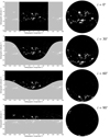 |
Fig. 5. Generation of solar-disk views for different inclination angles, indicated in the upper right corner of the panels and representing the number of degrees relative to the equator-on view (inclination of 0°). Left: Synoptic map illustrating the distribution of the entire solar surface around June 8, 2014. The shaded areas (gray part) mark the far side of the Sun. Right: Corresponding solar disk. The inclination of 90° corresponds to the Sun’s north pole-on view. |
3.4. Temporal evolution of the area fraction for different inclinations
Based on those generated solar-disk views (Fig. A.1), we built temporal series for each inclination by extracting the area fraction of the plages and enhanced network, called APEN following the method described in Vanden Broeck et al. (2024). For the whole USET dataset, we derived the area fraction for various inclinations from the equator-on view (i = 0° of latitude) to the pole-on view (i = 90° and i = −90°), as represented in Fig. 6. The plotted data are the monthly averaged data smoothed with a 13-month sliding window. There is an obvious lower peak-to-peak amplitude in the modulation of the area fraction when we move away from the equator-on point of view, in both hemispheres. At the minimum of the solar cycle, the variation of APEN between the equator-on view and the poles-on view is not significant. However, at the maximum, this variation is of 63% between the equator-on and north pole-on views, and 45% between the equator-on and south pole-on views. This is related to the apparent projected area of magnetic structures that are reduced by the foreshortening as observed from the poles. Despite the large change in amplitude at solar cycle maximum, the modulation associated with the solar cycle remains observable for both the north and south pole-on views. In the next section, we quantitatively analyze the impact of this variation on the detection of the temporal modulations.
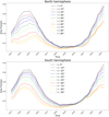 |
Fig. 6. Evolution of plages and enhanced network area fraction for different inclinations. Top panel: Inclinations from the equator-on view (i = 0° of latitude) to the north pole-on view (i = 90° of latitude). Bottom panel: Inclinations from the equator-on view to the south pole-on view (i = −90° of latitude). The data are the monthly averaged data smoothed with a 13-month sliding window. The colors stand for different inclinations. |
In addition, we observe that the curves for the two hemispheres peak at different times. The top panel of Fig. 7 shows the APEN time series for the polar view for each hemisphere. For the southern hemisphere (red curve), the solar maximum is clearly visible around mid-2014, while for the northern hemisphere, the solar maximum happens later, at the end of 2015. It is well-known that the solar activity presents significant asymmetries. This has been studied in detail in a variety of observations and activity indices, such as sunspot groups and areas, and sunspot numbers, but also for plages and flare occurrence (El-Borie et al. 2021; Veronig et al. 2021). The panels in Fig. 7 indeed show that, when separating the solar hemispheres, our time series of plages and enhanced network area fraction follow the same long-term evolution as the photospheric sunspot number, with the same variations of the north-south asymmetry. In Section 4, we will see that a corresponding asymmetry is naturally also found in the effects of inclination on our solar reconstructions.
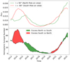 |
Fig. 7. Top panel: Comparison between the area fraction of plages and enhanced network, APEN, seen from the northern hemisphere (green) and from the southern hemisphere (red). The curves are the monthly averaged data smoothed with a 13-month sliding window. Bottom panel: International Sunspot Number (ISN), hemispheric 13-month smoothed number. Green parts represent an excess of activity in the northern hemisphere while red parts represent an excess in the southern hemisphere. Credit: SILSO (Royal Observatory of Belgium). |
4. Detection of temporal modulations out of the ecliptic
In this section, we analyze the time series of APEN for various inclinations more quantitatively. In particular, we use Fourier power spectra to look for the presence of periodic modulations on the solar cycle and solar rotation timescale. The discrete Fourier power spectrum method of Heck et al. (1985) and Gosset et al. (2001) was applied to each of the time series extracted for the 19 values of inclinations from i = −90° to i = +90° in steps of 10°. This Fourier methodology explicitly accounts for the uneven temporal sampling of astronomical time series such as those analyzed here. To assess the significance level of the peaks in the power spectrum, we used a bootstrapping method where the times of observations were kept fixed and the measured area fractions were redistributed randomly among the times of observations. For each reshuffled time series, we computed a power spectrum and determined the highest value of the power. The reshuffling process was repeated a thousand times for each inclination. The distribution of the highest peaks in the power spectra was used to determine the threshold corresponding to a 99% significance level, that is, 1% of the power spectra of the reshuffled time series have a higher power than this threshold.
Fig. 8 illustrates the power spectrum of the USET Ca II area fraction for an inclination of i = 0°. The top panel shows the logarithm of the power for frequencies below 0.05 d−1. The dashed blue horizontal line indicates the 99% significance level. The power spectrum is dominated by a peak at very low frequencies (see middle panel of Fig. 8). This peak is due to the long-term variations resulting from the 11-year solar cycle. As one can see, the group of peaks near the Carrington rotation frequency, νCar, (shown by the dashed magenta vertical line) is only marginally significant against the 99% significance level indicated by the blue line.
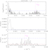 |
Fig. 8. Fourier power spectrum of the fractional area of the plages and enhanced network in the case of an inclination i = 0° (equator-on view). The upper and middle panels correspond to the power spectrum of the original data, while the lower panel gives the power spectrum of the time series detrended for the long-term cycle. The dashed blue lines in each panel illustrate the 99% significance level for the original time series, while the dashed red line in the bottom panel corresponds to the 99% significance level of the detrended time series. The magenta vertical lines in the top and bottom panels indicate the Carrington rotation frequency. |
4.1. Effect on the detection of the solar rotation
We then detrended the whole USET time series, removing the long-term modulation, and repeated the whole Fourier analysis and assessment of the significance level on the detrended time series. The power spectrum of the detrended data is shown in the bottom panel of Fig. 8, focusing on the region around the Carrington frequency. The dashed red line corresponds to the new 99% significance level for this detrended time series. One can clearly see that the group of peaks is now highly significant. The highest power is recorded at a frequency of 0.0383 d−1 (period of 26.1342 d), near the frequency of the equatorial synodic rotation period.
The highly complex structure of the peaks around the rotational frequency reflects the finite lifetime of the modulations which were most prominently seen during three distinct episodes of our USET time series (see Vanden Broeck et al. 2024). In the Fourier-transform framework, this finite lifetime requires the combination of multiple harmonic components at different frequencies near the base rotational frequency (multiple subpeaks). Together, the combined components will then reproduce the irregular amplitude modulation over the long timescales of the episodes with and without a detectable rotational signal. In addition, shifts in phase between the modulations at these different epochs play a role in the relative strengths of the various subpeaks of the structure.
Finally, Spörer’s law, which corresponds to the variation of heliographic latitudes of the active regions’ formation during the solar cycle, also affects the shape of the Fourier power spectrum around the rotational frequency. Indeed, because of the differential rotation, structures rotate faster near the equator. Hence, the detection of the modulation will be spread over a range of frequencies.
The rotational modulation arises from asymmetries in the longitudinal distribution of plages, as is explained in Vanden Broeck et al. (2024). Therefore, the frequency of the rotational modulation is set by the latitude at which such asymmetries appear, provided that their visibility changes with the rotation phase. For an inclination i > 0° (respectively, i < 0°), it is the regions between about 0° and −90° +i (respectively, 0° and 90° +i) for which the visibility changes most during the rotational cycle. As a result, for inclinations far away from an equator-on view, the most relevant frequency can be associated with active regions at latitudes in the other hemisphere as they undergo a substantial modulation of their visibility. One must keep in mind that this result reveals the role of asymmetry in the solar case. In the case of stars, it is impossible to determine whether or not asymmetry is present: it will simply manifest in one hemisphere or the other, playing a dominant role in the total signal. Therefore, the Sun provides an assessment of how a single hemisphere can differ from the other or from their sum, that is, the actual global level of stellar activity. From the stellar perspective, where one always observes the same hemisphere, the asymmetry between the data from the two solar hemispheres can be seen as two different realizations of the activity cycle.
Identical results to Fig. 8 for other inclinations from −90° to −90° are displayed in Appendix B. For inclinations between −20° and +20° (see Fig. B.1), the power spectra remain essentially identical. From |i|≥30° on, the amplitudes of the rotational modulation decrease as the absolute value of the inclination increases. We note a difference in behavior between the northern and southern inclinations: the group of peaks remains more important while moving toward the north pole-on view (i = +90°). In the southern hemisphere (negative inclinations), only one peak remains important. This behavior suggests that asymmetries in the longitudinal distribution of plages are stronger and thus more detectable in the southern hemisphere.
Finally, for |i|≥70°, the rotational modulation is no longer remarkable in the power spectrum and would certainly be missed in noisy and less densely sampled time series of other stars. Moreover, we observe a difference between both hemispheres. While the power spectrum for the southern hemisphere (inclination i = −70°) presents one clearly visible peak, the power spectrum for the northern hemisphere (inclination i = 70°) displays several peaks with the same power. An explanation of this behavior is again the asymmetry of the distribution of active regions between both hemispheres, as observed in Fig. 7. The distribution is not symmetric relative to the equator, so the visibility of the active regions is affected depending on the viewing angle. Indeed, for an inclination i = +70°, magnetic structures in the northern hemisphere down to a latitude of +20° will be visible over the entire rotation cycle, although with a changing aspect angle (sometimes closer to the limb, sometimes closer to the center of the disk). Therefore, these structures will not result in a strong rotational variation. Rotational modulation instead arises from active regions located at more southern latitudes. In our example, it is the negative latitudes, down to −20°, that will have the strongest impact. In our time series, the southern hemisphere hosts more active regions than the northern hemisphere during the solar maximum (see Fig. 7). Together with the finite lifetime of these active regions, the north-south asymmetry leads to the presence of multiple peaks in the power spectrum near the Carrington rotation frequency for i = +70°.
4.2. Effect on the detection of the solar cycle
To study the effect on the solar cycle timescale, we considered the power spectrum zoomed in at very low frequencies (middle panel of Fig. 8, illustrating the power spectrum for the view from the equator). We can clearly see the peak corresponding to the solar cycle modulation located at the frequency of about 0.00025 d−1, corresponding to a period of ∼10.95 years, analogous to the typical 11-year solar cycle. The dependence on inclination can be observed in Fig. B.1. The reduction in the power when the absolute value of the inclination increases is somewhat stronger for positive inclinations, but in both cases (positive or negative inclinations) the long-term modulation remains visible up to |i| = 90°, although with a significantly reduced power compared to an equator-on view.
4.3. Effect of the sampling
The USET Ca II K observations of the Sun benefit from a denser sampling than observations of other solar-like stars. Indeed, while the Sun can be observed throughout the year, the visibility of most stars is restricted to periods of, typically, 6 months. Moreover, whilst USET is dedicated to observations of the Sun, telescopes used for the study of chromospherically active stars usually have to share the observing time between a number of targets, resulting in a lower cadence of observations than for the USET data. This situation could bias the discussion of the detectability of the cyclic modulation as a function of inclination.
To account for this effect, we considered the sample of solar-like stars of Hempelmann et al. (2016), which are monitored with the TIGRE telescope, to search for rotational modulations and activity cycles in their S-index. We extracted the actual sampling of the TIGRE observations of these stars over the time period from 2013 until the end of 2023 from the TIGRE data archive. The number of observations ranges from less than 50 for the least-frequently observed star to over 400 for the most intensively observed targets. The mean and median numbers of observations for an individual star are both around 200, spread over this 10-year period. Fig. 9 illustrates the actual sampling and the spectral windows computed for a subset of these time series. The three stars that were chosen have a number of observations representative of the least-observed star, the mean number of observations, and the most frequently observed object. We note the yearly visibility gap. The spectral windows are dominated by the 1 d−1 alias. As one might expect, the spectral windows are cleaner when the number of data points increases. However, the most important difference compared to the time series of solar observations concerns the occurrence of a yearly alias at 0.00274 d−1, which can be seen by zooming in on the spectral windows (inset of the bottom panel of Fig. 9). This latter feature stems from the visibility constraints discussed above and can clearly be expected to impact the detectability of the long-term cycles. However, it should be emphasized that, due to its short duration, our time series is less favorable for the study of the long-duration cycle than some stellar time series. Indeed, our dataset only covers a single cycle. Consequently, the width of the peak in the Fourier power spectrum leads to a significant uncertainty in the actual period of the activity cycle. For other stars, even with a relatively sparse sampling, typically more than one activity cycle has been observed, therefore allowing a more accurate determination of the frequency associated with the long cycle.
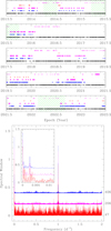 |
Fig. 9. Top: Temporal sampling of the USET data (black crosses) and the TIGRE observations of HD 10307 (blue squares), HD 17206 (magenta circles), and HD 1461 (red triangles). The latter three stars have been observed 47, 206, and 406 times, respectively, between 2013 and 2023. The hatched green areas highlight those time periods when the rotational modulation was strongest in the actual USET solar observations. Bottom: Spectral window of the time series of TIGRE observations of the same stars and using the same color code. The inset gives a zoom-in view of the low-frequency domain, illustrating the appearance of a yearly alias. The numbers on the right recall the total number of observations. |
We then sampled the time series of the USET plages and enhanced network areas for different inclinations, according to the sampling of the TIGRE observations of solar-like stars. Hereafter, we focus our discussion on the sampling corresponding to 206 observations spread over 10 years. Fig. 10 illustrates the Fourier power spectrum for an equator-on inclination for frequencies below 0.05 d−1, as well as around νCar. While the long-term cycle still provides the highest peak in the power spectrum, we note the presence of a strong yearly alias. With the sampling assumed here, the strongest peak remains the one associated with the long-term cycle. The situation is much worse as far as the detection of the rotational frequency is concerned. The sampling no longer allows an unambiguous identification of the dominant frequency that was found in the actual USET data. Indeed, there are now at least three peaks of equal strength around νCar, although all of them have a power well below the 99% significance level. But what is even worse is that there are a number of peaks at very different frequencies (e.g., near 0.009, 0.013, or 0.022 d−1) that have a power equal to or higher than that of the peaks near the actual rotation frequency. In a real stellar time series, one would thus not be able to identify the right frequency among those peaks. The situation remains essentially the same for other inclination angles (Fig. C.1). We thus conclude that a sampling of about 200 observations spread over 10 years would not allow a clear detection of the rotational modulation. This is not surprising given the fact that the visibility of the rotational modulation in the Sun’s plages and enhanced network area varies significantly with time, as shown in Vanden Broeck et al. (2024). A patchy sampling can thus easily miss those episodes where the rotational modulation would be well detected. For the long-term cycle, we observe that the peak associated with the true frequency remains the dominant one.
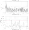 |
Fig. 10. Fourier power spectrum of the resampled USET time series, assuming 206 observations spread over 10 years for an equator-on view. The top panel illustrates the logarithm of the power spectrum for frequencies below 0.05 d−1. The long-dashed blue line marks the 99% significance level. The bottom panel provides a zoom-in on the power spectrum around νCar (given by the short-dashed magenta vertical line) after removing the long-term trend from the data. The long-dashed red line indicates the 99% significance level for the detrended time series. The magenta vertical lines in the top and bottom panels indicate the Carrington rotation frequency. |
As a next step, we resampled the USET plages and enhanced network area time series for inclinations of +30° and −30° according to the observing cadence of ten representative stars of the TIGRE sample of Hempelmann et al. (2016). The results of this exercise are illustrated in Fig. D.1 for the sampling used for three stars with 405, 206, and 47 observations over 10 years.
Although the long-term cycle is detected in all cases, one can clearly see that the contrast of the peak with respect to the 99% significance level strongly decreases when the sampling gets sparser, as expected. The ratio between the power of the highest peak and the 99% significance level decreases from 14 for the densest sampling to 8 for the intermediate case and 1.6 for the sparsest case. Hence, we conclude that a long-term cycle with an amplitude identical to that of the Sun would remain detectable with a sampling of ∼20 observations per year, provided that the data covered a sufficiently long time interval. As expected, the significance level decreases when the number of observations decreases, becoming marginal for the sparsest sampling (a handful of observations per year). Concerning the rotational modulation, we note that the corresponding peaks are now only marginally above the 99% level after prewhitening the long-term variations (see Fig. 10). This is partially due to the fact that the sampling overlaps only partially with one of the epochs where the rotational signature in the original USET data was prominently seen (see Fig. 9). Shifting the time series by 180 days somewhat improves the overlap, but the detectability of the rotational signature remains marginal because of an insufficiently dense sampling of the data.
Finally, to assess the impact of the amplitude of the cyclic variations on their detectability with a typical sampling of solar-like stars, we performed another set of simulations. We first adjusted the long-term cycle variations for each set of simulated out-of-ecliptic USET data (i.e., for each value of the inclination) by a polynomial of degree six as we had done for the actual USET observations in Vanden Broeck et al. (2024). Subtracting this polynomial from the simulated time series yields a proxy of the shorter-term variations. We then scaled the amplitude of the adjusted long-term cycle by a factor between 0.1 and 10.0 (in logarithmic steps of logAmpcyc/AmpUSET = −0.5). These scaled long-term variations were then added back to the shorter-term variations to simulate situations of solar-like stars with different ratios between the amplitudes of the short- and long-term variations. These simulated time series were then resampled with our reference observing cadence of 206 observations spread over 10 years, as well as with the two most extreme cadences (47 and 406 observations spread over 10 years). Fig. 11 illustrates the results of this exercise. The colors indicate the ratio between the power of the strongest peak in the Fourier spectrum that is associated with the long-term cycle and the power corresponding to the 99% significance level. As one might expect, the detectability of the long-term cycle is strongly impacted by the sampling. For the lowest sampling, the ratio of the highest power never exceeds three times the power corresponding to the 99% significance level, even when the amplitude of the cycle is scaled by a factor of ten. Conversely, for the densest sampling studied here, the power of the highest peak exceeds seven times that of the 99% significance level, even when the amplitude of the cycle is reduced by half. The detectability becomes marginal (ratio lower than 2 or even 1, red and orange colors in Fig. 11) when the amplitude of the cycle is scaled down by a factor of 0.1. With our reference sampling of 206 data points over 10 years, the peak due to the long-term cycle is detected at a level at least three times above the 99% significance level, provided that the amplitude of the cyclic variations remains at a level of at least 33% of the amplitude seen in the USET data. For lower values, the detections become uncertain too, because the highest peaks in the Fourier spectra are no longer necessarily associated with the frequency of the long-term cycle.
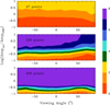 |
Fig. 11. Detectability of the long-term cycle as a function of the viewing angle and the scaled amplitude of the long-term cycle. The different panels correspond to different samplings, with the number of data points taken over 10 years indicated in each panel. The color scale to the right indicates the ratio between the power of the peak associated with the long-term cycle in the Fourier power spectrum and the power corresponding to the 99% significance level. |
We note that the visibility of the peak displays some variation with inclination. This results from a combination of different effects. First, the power corresponding to the 99% significance level results from the combination of all types of variation (cyclic, rotational, and stochastic fluctuations). It reaches the highest values for viewing angles between −10° and +10°. Hence, this denominator of the quantity illustrated in Fig. 11 does not scale simply with the amplitude of the cycle. Moreover, as shown by Fig. 7, there exists an asymmetry between the northern and southern solar hemispheres in our data. The southern variations have a more sinusoidal shape, implying that most of the power of the cyclic variations will be concentrated in a single peak. The situation is quite different for the northern hemisphere, where the variations display several peaks, implying that the power is split between the fundamental frequency and its harmonics. But, above all, Fig. 11 shows that these trends depend strongly on the details of the actual sampling. Therefore, the variations with inclination should not be overinterpreted.
5. Discussion and conclusions
Based on full-disk images of the solar chromosphere in the Ca II K line from the USET station, we mapped the solar surface with synoptic maps. We segmented the brightest structures and produced a time series of their area fraction. Then we used an appropriate projection to represent the solar surface as it would be seen under various viewing angles. We computed the area fraction for different inclinations and its variation goes up to 63% between the equator-on view and the poles-on view during the maximum of the solar cycle.
As the plages and enhanced network area fraction is a good proxy for the S-index (Vanden Broeck et al. 2024), this study can be used to make a connection between the Sun and other Sun-like stars. In particular, it could be used to better understand the detection of temporal modulation for the other stars that are not necessarily viewed from the equator plane. To reach this goal, we analyzed the impact of the viewing angle on the area fraction time series by using Fourier power spectra.
Our results show an important impact of the viewing angle on the detection of modulation due to solar rotation. If the observations use the same (dense) sampling as the USET data, the rotation is detectable up to an inclination of |i| = 70°. For higher values, the rotation is no longer visible in the signal and would be missed. This behavior could be explained by the fact that, from a pole-on view, an asymmetry in the plages distribution will be either permanently visible or not visible at all during a full solar rotation cycle.
In the long term, the chromospheric activity cycles of Sun-like stars should remain detectable even for stars seen at a near pole-on viewing angle. Positive and negative inclinations give different results due to the asymmetry of the solar activity in the northern and southern hemispheres, as already seen for other magnetic structures.
For other stars, the actual detectability will also depend on the sampling of the time series and on the quality of the data. Indeed, our USET time series benefits from a long continuous time series with dense sampling. Actual time series of stellar S-indices usually have more complicated and scarcer samplings, including months-long gaps due to restricted target visibility. We analyzed the effect of the sampling on the detection of the periodic modulations by extracting the actual sampling of TIGRE observations of Sun-like stars over a period of 10 years. The least frequently observed star is observed fewer than 50 times, while the most intensively observed one has over 400 observations. We demonstrate that a more realistic sampling leads to the rotational modulation detection vanishing. However, the modulation due to the activity cycle remains visible at nearly all inclinations if the sampling contains at least 20 observations per year and as long as the amplitude of the cyclic variation is at least 30% of the solar cycle amplitude. This conclusion is made on the assumption of a typical solar activity case (i.e., of ∼11 years). In the case of stars with a much shorter or much longer cycle than the solar cycle, the period of the activity cycle will be very difficult to determine because of the sparsity of the sampling. Indeed, for significantly longer cycles, we would need a much longer homogeneous dataset, which is hard to collect for stellar observations. For shorter cycles (of a few months, e.g., Mittag et al. 2019), the sparse sampling assumed here would clearly fail to correctly identify the exact cycle duration.
While we consider a fixed cycle length of 11 years, Meunier et al. (2023) explicitly study the impact of cycle length on cycle period estimation. Their study is based on a large sample of synthetic time series produced from a large set of physical parameters (Meunier et al. 2019). In Meunier et al. (2023) they considered a subsample of time series with a duration longer than 10 years and 1000 nights of observations randomly spread over the sampling. Then they compared the reconstructed time series period with the true one. They show that, for cycle periods of about 3 and 6 years, the estimation of the cycle period is quite accurate, but for a cycle period of 12 years, the uncertainty increases. In addition, they show that the reconstruction is better for higher cycle amplitudes. An extension of our present study would clearly benefit from a dataset covering a longer time span, as the impact of the inclination axis may vary with the solar cycle amplitude (Sowmya et al. 2021).
Acknowledgments
The authors wish to thank Sowmya Krishnamurthy from the Max Planck Institute for Solar Research System, in Germany, for the very productive discussions that enabled them to carry out the work on the orthographic projection. Grégory Vanden Broeck was supported by a PhD grant awarded by the Royal Observatory of Belgium. The USET instruments are built and operated with the financial support of the Solar-Terrestrial Center of Excellence (STCE).
References
- Baliunas, S. L., Horne, J. H., Porter, A., et al. 1985, ApJ, 294, 310 [Google Scholar]
- Baliunas, S. L., Donahue, R. A., Soon, W., & Henry, G. W. 1998, ASP Conf. Ser., 154, 153 [Google Scholar]
- Bechet, S., & Clette, F. 2002, USET Images L1centered (Royal Observatory of Belgium (ROB)), https://doi.org/10.24414/nc7j-b391 [Google Scholar]
- Borgniet, S., Meunier, N., & Lagrange, A. M. 2015, A&A, 581, A133 [NASA ADS] [CrossRef] [EDP Sciences] [Google Scholar]
- Boro Saikia, S., Marvin, C. J., Jeffers, S. V., et al. 2018, A&A, 616, A108 [NASA ADS] [CrossRef] [EDP Sciences] [Google Scholar]
- Calabretta, M. R., & Greisen, E. W. 2002, A&A, 395, 1077 [NASA ADS] [CrossRef] [EDP Sciences] [Google Scholar]
- Devi, P., Singh, J., Chandra, R., Priyal, M., & Joshi, R. 2021, Sol. Phys., 296, 49 [Google Scholar]
- El-Borie, M., El-Taher, A., Thabet, A., Ibrahim, S., & Bishara, A. 2021, Chin. J. Phys., 72, 1 [Google Scholar]
- Gosset, E., Royer, P., Rauw, G., Manfroid, J., & Vreux, J. M. 2001, MNRAS, 327, 435 [NASA ADS] [CrossRef] [Google Scholar]
- Heck, A., Manfroid, J., & Mersch, G. 1985, A&AS, 59, 63 [NASA ADS] [Google Scholar]
- Hempelmann, A., Mittag, M., Gonzalez-Perez, J. N., et al. 2016, A&A, 586, A14 [NASA ADS] [CrossRef] [EDP Sciences] [Google Scholar]
- Knaack, R., Fligge, M., Solanki, S. K., & Unruh, Y. C. 2001, A&A, 376, 1080 [NASA ADS] [CrossRef] [EDP Sciences] [Google Scholar]
- Lockwood, G. W., & Skiff, B. A. 1990, NASA Conf. Publ., 3086, 8 [Google Scholar]
- Lockwood, G. W., Skiff, B. A., Henry, G. W., et al. 2007, ApJS, 171, 260 [Google Scholar]
- Met Office 2010–2015, Cartopy: A Cartographic Python Library with a Matplotlib Interface, https://scitools.org.uk/cartopy [Google Scholar]
- Meunier, N., Lagrange, A. M., Boulet, T., & Borgniet, S. 2019, A&A, 627, A56 [NASA ADS] [CrossRef] [EDP Sciences] [Google Scholar]
- Meunier, N., Pous, R., Sulis, S., Mary, D., & Lagrange, A.-M. 2023, A&A, 676, A82 [NASA ADS] [CrossRef] [EDP Sciences] [Google Scholar]
- Meunier, N., Lagrange, A. M., Dumusque, X., & Sulis, S. 2024, A&A, 687, A303 [NASA ADS] [CrossRef] [EDP Sciences] [Google Scholar]
- Mittag, M., Schröder, K. P., Hempelmann, A., González-Pérez, J. N., & Schmitt, J. H. M. M. 2016, A&A, 591, A89 [NASA ADS] [CrossRef] [EDP Sciences] [Google Scholar]
- Mittag, M., Schmitt, J. H. M. M., Hempelmann, A., & Schröder, K. P. 2019, A&A, 621, A136 [NASA ADS] [CrossRef] [EDP Sciences] [Google Scholar]
- Mittag, M., Schmitt, J. H. M. M., & Schröder, K. P. 2023, A&A, 674, A116 [NASA ADS] [CrossRef] [EDP Sciences] [Google Scholar]
- Nèmec, N. E., Shapiro, A. I., Krivova, N. A., et al. 2020, A&A, 636, A43 [Google Scholar]
- Noyes, R. W., Hartmann, L. W., Baliunas, S. L., Duncan, D. K., & Vaughan, A. H. 1984, ApJ, 279, 763 [Google Scholar]
- Radick, R. R., Lockwood, G. W., Henry, G. W., Hall, J. C., & Pevtsov, A. A. 2018, ApJ, 855, 75 [Google Scholar]
- Reinhold, T., Shapiro, A. I., Solanki, S. K., et al. 2020, Science, 368, 518 [Google Scholar]
- Schatten, K. H. 1993, J. Geophys. Res., 98, 18907 [NASA ADS] [CrossRef] [Google Scholar]
- Shapiro, A. I., Solanki, S. K., Krivova, N. A., et al. 2014, A&A, 569, A38 [NASA ADS] [CrossRef] [EDP Sciences] [Google Scholar]
- Singh, J., Priyal, M., Ravindra, B., Bertello, L., & Pevtsov, A. 2023, Res. Astron. Astrophys., 23, 045016 [CrossRef] [Google Scholar]
- Sowmya, K., Shapiro, A. I., Witzke, V., et al. 2021, ApJ, 914, 21 [CrossRef] [Google Scholar]
- Vanden Broeck, G., Bechet, S., Clette, F., et al. 2024, A&A, 689, A95 [NASA ADS] [CrossRef] [EDP Sciences] [Google Scholar]
- Vaughan, A. H., Baliunas, S. L., Middelkoop, F., et al. 1981, ApJ, 250, 276 [NASA ADS] [CrossRef] [Google Scholar]
- Veronig, A. M., Jain, S., Podladchikova, T., Pötzi, W., & Clette, F. 2021, A&A, 652, A56 [NASA ADS] [CrossRef] [EDP Sciences] [Google Scholar]
- Wilson, O. C. 1978, ApJ, 226, 379 [Google Scholar]
- Wright, J. T., Marcy, G. W., Butler, R. P., & Vogt, S. S. 2004, ApJS, 152, 261 [Google Scholar]
Appendix A: Generation of solar-disk views for different inclinations.
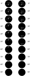 |
Fig. A.1. Distribution of the segmented structures with the generated solar-disk views on 1st of August 2014 for inclinations from 0° of latitude to 90° and −90° of latitude by steps of 10°. Inclination angles are specified next to each image and represent the number of degrees relative to the equator-on view (i = 0°). Top images illustrate the view from the equator and it goes to the south pole view (left) and to the north pole view (right). |
Appendix B: Fourier power spectra for different inclinations
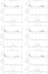 |
Fig. B.1. Same as Fig. 8, but for inclinations of −90° to 90°. The upper and middle panels correspond to the power spectrum of the original data, whilst the lower panel yields the power spectrum of the time series detrended for the long-term cycle. The blue dashed lines in each panel illustrate the 99% significance level for the original time series, whilst the red dashed line in the bottom panel corresponds to the 99% significance level of the detrended time series. The magenta vertical lines in the top and bottom panel indicate the Carrington rotation frequency. |
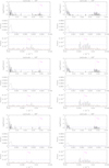 |
Fig. B.1. Continued |
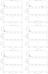 |
Fig. B.1. Continued |
Appendix C: Fourier power spectrum of the resampled USET time series assuming 206 observations spread over ten years for different viewing angles
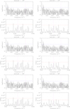 |
Fig. C.1. The top panels illustrate the logarithm of the power spectrum for frequencies below 0.05 d−1. The bottom panels provide a zoom-in on the power around the Carrington rotation frequency νCar (given by the magenta vertical lines). The dashed horizontal lines illustrate the 99% significance level, the blue one for the original time series and the red one for the detrended time series. |
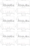 |
Fig. C.1. Continued |
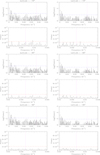 |
Fig. C.1. Continued |
Appendix D: Fourier power spectrum of the resampled USET time series for different observing cadence
 |
Fig. D.1. Fourier power spectrum of the resampled USET time series for a decreasing observing cadence (from top to bottom) and for inclination angles of +30° (left column) and −30° (right column row). For each case, the top panel illustrates the logarithm of the power spectrum for frequencies below 0.05 d−1 and the bottom panel provides a zoom-in on the power around νCar (given by the short-dashed green vertical line). The long-dashed blue horizontal line yields the 99% significance level. |
All Figures
|
Fig. 1. Correlation between daily values of the solar S-index from TIGRE (in the Mount Wilson scale) and the USET area fraction of plages and enhanced network, APEN. The parameter n represents the number of data, and the chronological order is color coded. The first and last dates of the data are given next to the color bar. Additionally, a linear fit to the data was performed (solid red line). A mean error bar is displayed in the bottom right corner to give an idea of the uncertainties on the data. Image taken from Vanden Broeck et al. (2024). |
| In the text | |
|
Fig. 2. Example of the segmentation process. Left: Recentered raw image from October 29, 2013. Right: Result of the segmentation. |
| In the text | |
|
Fig. 3. Example of a CAR projection. Left: Raw solar image. Right: Corresponding image after the projection. |
| In the text | |
|
Fig. 4. Example of a segmented synoptic map built around July 7, 2014, illustrating the distribution of the plages and enhanced network during a full solar rotation. The x-axis represents the number of degrees of longitude from the Carrington longitude on July 7, 2014 (center of image). |
| In the text | |
|
Fig. 5. Generation of solar-disk views for different inclination angles, indicated in the upper right corner of the panels and representing the number of degrees relative to the equator-on view (inclination of 0°). Left: Synoptic map illustrating the distribution of the entire solar surface around June 8, 2014. The shaded areas (gray part) mark the far side of the Sun. Right: Corresponding solar disk. The inclination of 90° corresponds to the Sun’s north pole-on view. |
| In the text | |
|
Fig. 6. Evolution of plages and enhanced network area fraction for different inclinations. Top panel: Inclinations from the equator-on view (i = 0° of latitude) to the north pole-on view (i = 90° of latitude). Bottom panel: Inclinations from the equator-on view to the south pole-on view (i = −90° of latitude). The data are the monthly averaged data smoothed with a 13-month sliding window. The colors stand for different inclinations. |
| In the text | |
|
Fig. 7. Top panel: Comparison between the area fraction of plages and enhanced network, APEN, seen from the northern hemisphere (green) and from the southern hemisphere (red). The curves are the monthly averaged data smoothed with a 13-month sliding window. Bottom panel: International Sunspot Number (ISN), hemispheric 13-month smoothed number. Green parts represent an excess of activity in the northern hemisphere while red parts represent an excess in the southern hemisphere. Credit: SILSO (Royal Observatory of Belgium). |
| In the text | |
|
Fig. 8. Fourier power spectrum of the fractional area of the plages and enhanced network in the case of an inclination i = 0° (equator-on view). The upper and middle panels correspond to the power spectrum of the original data, while the lower panel gives the power spectrum of the time series detrended for the long-term cycle. The dashed blue lines in each panel illustrate the 99% significance level for the original time series, while the dashed red line in the bottom panel corresponds to the 99% significance level of the detrended time series. The magenta vertical lines in the top and bottom panels indicate the Carrington rotation frequency. |
| In the text | |
|
Fig. 9. Top: Temporal sampling of the USET data (black crosses) and the TIGRE observations of HD 10307 (blue squares), HD 17206 (magenta circles), and HD 1461 (red triangles). The latter three stars have been observed 47, 206, and 406 times, respectively, between 2013 and 2023. The hatched green areas highlight those time periods when the rotational modulation was strongest in the actual USET solar observations. Bottom: Spectral window of the time series of TIGRE observations of the same stars and using the same color code. The inset gives a zoom-in view of the low-frequency domain, illustrating the appearance of a yearly alias. The numbers on the right recall the total number of observations. |
| In the text | |
|
Fig. 10. Fourier power spectrum of the resampled USET time series, assuming 206 observations spread over 10 years for an equator-on view. The top panel illustrates the logarithm of the power spectrum for frequencies below 0.05 d−1. The long-dashed blue line marks the 99% significance level. The bottom panel provides a zoom-in on the power spectrum around νCar (given by the short-dashed magenta vertical line) after removing the long-term trend from the data. The long-dashed red line indicates the 99% significance level for the detrended time series. The magenta vertical lines in the top and bottom panels indicate the Carrington rotation frequency. |
| In the text | |
|
Fig. 11. Detectability of the long-term cycle as a function of the viewing angle and the scaled amplitude of the long-term cycle. The different panels correspond to different samplings, with the number of data points taken over 10 years indicated in each panel. The color scale to the right indicates the ratio between the power of the peak associated with the long-term cycle in the Fourier power spectrum and the power corresponding to the 99% significance level. |
| In the text | |
|
Fig. A.1. Distribution of the segmented structures with the generated solar-disk views on 1st of August 2014 for inclinations from 0° of latitude to 90° and −90° of latitude by steps of 10°. Inclination angles are specified next to each image and represent the number of degrees relative to the equator-on view (i = 0°). Top images illustrate the view from the equator and it goes to the south pole view (left) and to the north pole view (right). |
| In the text | |
|
Fig. B.1. Same as Fig. 8, but for inclinations of −90° to 90°. The upper and middle panels correspond to the power spectrum of the original data, whilst the lower panel yields the power spectrum of the time series detrended for the long-term cycle. The blue dashed lines in each panel illustrate the 99% significance level for the original time series, whilst the red dashed line in the bottom panel corresponds to the 99% significance level of the detrended time series. The magenta vertical lines in the top and bottom panel indicate the Carrington rotation frequency. |
| In the text | |
|
Fig. B.1. Continued |
| In the text | |
|
Fig. B.1. Continued |
| In the text | |
|
Fig. C.1. The top panels illustrate the logarithm of the power spectrum for frequencies below 0.05 d−1. The bottom panels provide a zoom-in on the power around the Carrington rotation frequency νCar (given by the magenta vertical lines). The dashed horizontal lines illustrate the 99% significance level, the blue one for the original time series and the red one for the detrended time series. |
| In the text | |
|
Fig. C.1. Continued |
| In the text | |
|
Fig. C.1. Continued |
| In the text | |
|
Fig. D.1. Fourier power spectrum of the resampled USET time series for a decreasing observing cadence (from top to bottom) and for inclination angles of +30° (left column) and −30° (right column row). For each case, the top panel illustrates the logarithm of the power spectrum for frequencies below 0.05 d−1 and the bottom panel provides a zoom-in on the power around νCar (given by the short-dashed green vertical line). The long-dashed blue horizontal line yields the 99% significance level. |
| In the text | |
Current usage metrics show cumulative count of Article Views (full-text article views including HTML views, PDF and ePub downloads, according to the available data) and Abstracts Views on Vision4Press platform.
Data correspond to usage on the plateform after 2015. The current usage metrics is available 48-96 hours after online publication and is updated daily on week days.
Initial download of the metrics may take a while.