| Issue |
A&A
Volume 697, May 2025
|
|
|---|---|---|
| Article Number | A115 | |
| Number of page(s) | 16 | |
| Section | Interstellar and circumstellar matter | |
| DOI | https://doi.org/10.1051/0004-6361/202554067 | |
| Published online | 19 May 2025 | |
Metallicity dependence of the CO-to-H2 and the [CI]-to-H2 conversion factors in galaxies
1
Research Center for Astronomical Computing, Zhejiang Laboratory,
Hangzhou
311000,
China
2
School of Astronomy and Space Science, Nanjing University,
Nanjing
210093,
China
3
Key Laboratory of Modern Astronomy and Astrophysics (Nanjing University), Ministry of Education,
Nanjing
210093,
China
4
Department of Physics, Aristotle University of Thessaloniki,
Greece
5
Institut de Radioastronomie Millimétrique,
300 rue de la Piscine,
38400
Saint-Martin-d’Héres,
France
6
Yunnan Observatories, Chinese Academy of Sciences,
Kunming
650011,
China
7
Key Laboratory of Radio Astronomy and Technology (Chinese Academy of Sciences),
A20 Datun Road,
Chaoyang District, Beijing
100101,
PR China
8
I. Physikalisches Institut, Universität zu Köln,
Zülpicher Straße 77,
50937
Köln,
Germany
9
New Cornerstone Science Laboratory, Department of Astronomy, Tsinghua University,
Beijing
100084,
China
10
National Astronomical Observatories, Chinese Academy of Sciences,
Beijing
100101,
China
★ Corresponding authors: This email address is being protected from spambots. You need JavaScript enabled to view it.
; This email address is being protected from spambots. You need JavaScript enabled to view it.
Received:
7
February
2025
Accepted:
14
March
2025
Abstract
Understanding the molecular gas content in the interstellar medium (ISM) is crucial for studying star formation and galaxy evolution. The CO-to-H2 (XCO) and the [CI]-to-H2 (XCI) conversion factors are widely used to estimate the molecular mass content in galaxies. However, these factors depend on many environmental parameters in the ISM, such as metallicity, cosmic-ray ionization rate, and far-ultraviolet (FUV) radiation field, in particular, in the low-metallicity ISM that is found at large galactocentric radii and in early-type galaxies. This work investigates the dependence of XCO and XCI on the environmental parameters of the ISM, with a focus on the low-metallicity α-enhanced ISM ([C/O] < 0), to provide improved tracers of molecular gas under diverse conditions. We used the statistical algorithm PDFCHEM, coupled with a database of photodissociation region (PDR) models generated with the 3D-PDR astrochemical code. The models account for a wide range of metallicities, dust-to-gas mass ratios, FUV intensities, and cosmic-ray ionization rates. The conversion factors were computed by integrating the PDR properties over log-normal column density distributions (AV-PDFs) that represent various cloud types. The XCO factor increases significantly with decreasing metallicity. It exceeds ∼1000 times the Galactic value at [O/H] = −1.0 under α-enhanced conditions, as opposed to ∼300 times under non-α-enhanced conditions ([C/O] = 0). In contrast, XCI varies more gradually with metallicity, which makes it a more reliable tracer of molecular gas in metal-poor environments under most conditions. The fraction of CO-dark molecular gas increases dramatically in low-metallicity regions, where it exceeds 90% at [O/H] = −1.0, in particular, in diffuse clouds and environments with strong FUV radiation fields. The results highlight the limitations of CO as a molecular gas tracer in the metal-poor ISM and demonstrate the potential of [CI] (1–0) as a complementary tracer. The use of metallicity-dependent XCO and XCI factors as provided by this study is recommended for accurately estimating molecular gas masses in diverse environments. We recommend the use of the log10 XCO ≃ −2.41 Z + 41.3 relation for the CO-to-H2 conversion factor and the log10 XCI ≃ −0.99 Z + 29.7 relation for the [CI]-to-H2 conversion factor, where Z = 12 + log10(O/H).
Key words: astrochemistry / radiative transfer / methods: numerical / ISM: general / photon-dominated region (PDR)
© The Authors 2025
 Open Access article, published by EDP Sciences, under the terms of the Creative Commons Attribution License (https://creativecommons.org/licenses/by/4.0), which permits unrestricted use, distribution, and reproduction in any medium, provided the original work is properly cited.
This article is published in open access under the Subscribe to Open model. This email address is being protected from spambots. You need JavaScript enabled to view it. to support open access publication.
1 Introduction
Determining the molecular gas content in galaxies is fundamental for understanding the evolution of the interstellar medium (ISM) and the star formation process across cosmological epochs. The H2 molecule, however, is difficult to observe directly in the cold (Tgas ∼10 K) and dense (nH ≳ 103 cm−3) ISM state where stars form, since its first two rotational transitions have upper-level energies of about E/kB ≃ 510 K and 1015 K, respectively (Dabrowski 1984). Observations conducted to determine the existence of the cold molecular gas therefore rely on the emission that is captured by other tracers. In this regard, the molecule of 12CO (hereafter referred to as CO) is perhaps the most commonly used because it is highly abundant in molecular clouds (∼10−4 at Z = 1 Z⊙, Sofia et al. 2004). Its J = 1−0 transition has a low excitation energy barrier ΔE/k ∼5 K and low critical density of ∼2.2 × 103 cm−3 (Bolatto et al. 2013), which means that it is easily excited in cold environments (Scoville et al. 2016). This emission line is then converted into an H2 column density using the simple expression N(H2)=XCO. WCO 1−0, where XCO is the conversion factor (or ‘XCO-factor’, see review by Bolatto et al. 2013) and WCO 1−0 is the velocity-integrated line emission of CO (1–0). For typical Milky Way (MW) conditions, the value of XCO = 2 × 1020 cm−2 (K km s−1)−1 with a ±30% variation is usually adopted (Strong & Mattox 1996; Dame et al. 2001; Bell et al. 2007; Szűcs et al. 2016; Bisbas et al. 2021; Skalidis et al. 2024).
The transition from atomic hydrogen to molecular hydrogen (frequently called HI-to-H2 transition) is a vital first step in the process of star formation. When a cold (Tgas ≲ 30 K) atomic cloud is sufficiently shielded from the interstellar ultraviolet radiation (UV) field, the H2 molecule (which mainly forms on dust grains) can no longer be photodissociated. This rapidly increases the H2 abundance and creates the conditions in which the star formation process can begin (see review by McKee & Ostriker 2007). While extreme-ultraviolet (EUV) radiation (hv ≥ 13.6 eV) predominates in the vicinity of massive stars, far-ultraviolet (FUV) radiation (6 ≲ hv < 13.6 eV) governs the physical and chemical processes in photodissociation regions (‘PDRs’, see reviews by Hollenbach & Tielens 1999; Tielens 2005; Wolfire et al. 2022). The H2 formation rate coefficient and the dust absorption cross section are both proportional to metallicity (Sternberg et al. 2014). Therefore, as the metallicity increases, the transition from HI to H2 shifts to lower column densities because the dust-to-gas mass ratio increases.
From the theory of PDRs, it is known that H2 typically forms at lower visual extinctions than CO because of its self-shielding ability (Tielens & Hollenbach 1985). A certain region is then H2 rich but CO poor (Lada & Blitz 1988), which leads to the socalled CO-dark molecular gas (van Dishoeck 1990, 1992). The term CO-dark gas was coined because the H2-rich gas cannot be observed by the above line emission. Consequently, this has a direct impact on the accuracy of the H2 gas mass that is determined through the CO (1−0) millimeter line (see e.g. Gong et al. 2018, 2020; Bigiel et al. 2020; Luo et al. 2020; Seifried et al. 2020; Bisbas et al. 2021; Dunne et al. 2021, 2022; Hu et al. 2022; Borchert et al. 2022, for recent developments). Alternative tracers have been proposed in this regard that include the [CI] 3P1 → 3P0 at 609 μm (hereafter, [CI] (1–0); e.g., Papadopoulos et al. 2004) and the [CII] 158 μm (e.g. Zanella et al. 2018; Zhao et al. 2024) lines of the carbon cycle (C+/C/CO), which are popular in particular because of the sensitivity of the Atacama Large Millimeter/submillimeter Array (ALMA) interferometry in these lines, especially when studying high-redshift galaxies.
The [CI] (1–0) line was proposed as an alternative and accurate H2 tracer more than two decades ago (Papadopoulos et al. 2004) because it is more optically thin than CO (1–0) and has a low excitation temperature of ΔE/k ∼24 K. The validity of using [CI](1−0) in measuring the molecular gas mass was confirmed by subsequent observational (Lo et al. 2014; Jiao et al. 2017, 2019, 2021; Crocker et al. 2019; Heintz & Watson 2020; Dunne et al. 2021, 2022) and numerical works (Offner et al. 2014; Glover et al. 2015; Glover & Clark 2016; Papadopoulos et al. 2018; Gaches et al. 2019; Bisbas et al. 2021). Atomic carbon forms as long as the HI-to-H2 transition occurs (Röllig et al. 2007; Wolfire et al. 2022), which closely links the [CI] (1–0) line with the CO-dark gas. In the classical picture, the C-rich layer is always thought to be a thin layer (e.g. Tielens 2005). However, recent theoretical models studying ISM environments with enhanced cosmic-ray energy densities (Bialy et al. 2015; Bisbas et al. 2015, 2017a) showed that the C-rich layer is a rather extended region that covers a wide density range that consists of cold H2-rich gas. Three-dimensional PDR modeling (Bisbas et al. 2021) showed that the additional gas heating through the higher cosmic-ray ionization rate (ζCR) results in [CI]- and also [CII]-bright molecular gas.
Both 12C and 16O are products of stellar nucleosynthesis, but they are released in the ISM through different mechanisms (see Romano 2022, for a review). In particular, 16O is released through type II supernova explosions from the massive M ≳ 8 M⊙ short-lived stars. On the other hand, 12C is mainly released through type Ia supernovae of low- and intermediate-mass stars (1 < M < 8 M⊙), which live much longer. Throughout the stellar evolution within a galaxy, these differential release mechanisms cause a nonlinear relation between the abundances of C and O (Trainor et al. 2016; Cooke et al. 2017; Berg et al. 2016, 2019; Maiolino & Mannucci 2019). This was specifically studied by Berg et al. (2019), who conducted chemical evolution models to explain that the observed trend of C/O versus O/H in metal-poor dwarf galaxies is a product of the detailed star formation history and supernova feedback. Environments that contain lower-than-expected C/O values from the typical solar (linear) scaling are therefore characterized by the relative enrichment of oxygen, the most typical α element. These environments are therefore known as α-enhanced environments.
The C/O abundance is not the only abundance that scales differentially with O/H. The dust-to-gas (DTG) mass ratio is another important parameter in the evolution of the cosmic ISM (Hunter et al. 2024). A lower DTG in the metal-poor ISM was observed by various groups (e.g. Galametz et al. 2011; Magdis et al. 2011, 2012; Herrera-Camus et al. 2012; Sandstrom et al. 2013; Rémy-Ruyer et al. 2014; Shapley et al. 2020; Galliano et al. 2021; Popping & Péroux 2022; Yasuda et al. 2023; Konstantopoulou et al. 2024), which provided various scaling relations with O/H. Chemical evolution models of the Galaxy showed that dust grows via the accretion of metals after a certain critical metallicity value has been reached (Asano et al. 2013a,b), while type-II supernovae increase the DTG during starburst events (Zhukovska 2014). These dust evolution approaches were further explored in recent numerical models such as the DustySAGE (Triani et al. 2020) and the Feedback In Realistic Environments (FIRE) galactic simulations by Choban et al. (2024), which provided a more complete picture of dust growth in various galaxy types.
A more detailed impact of the nonlinear C/O and DTG ratios as a function of O/H on the abundances and line emission of the carbon cycle was studied by Bisbas et al. (2024). Their three-dimensional PDR modeling showed that α-enhanced metal-poor galaxies may appear to be bright in low-J CO emission lines, but dark in [CI] lines (in agreement with recent observations of [CI]-dark galaxies, e.g. Michiyama et al. 2020, 2021; Harrington et al. 2021; Dunne et al. 2022; Lelli et al. 2023) and possibly in the [CII] 158 μm line. In addition, Bisbas et al. (2024) reported that in these α-enhanced environments, low-J CO lines appear to be the most stable lines for tracing molecular gas. The main conclusion of that work was that the C/O ratio cannot be neglected in astrochemical models as it constitutes an important environmental parameter of the ISM.
The impact of metallicity variations on the conversion factors was addressed and studied in various observations (e.g. Leroy et al. 2011; Schruba et al. 2012; Genzel et al. 2012; Sandstrom et al. 2013; Hunt et al. 2015; Amorín et al. 2016; Madden et al. 2020) and numerical models (e.g. Accurso et al. 2017; Bisbas et al. 2021; Hu et al. 2021; Ramambason et al. 2024). In general, it was found that the XCO conversion factor increases with decreasing metallicity with respect to the average MW value, while it decreases toward higher-metallicity regions, such as the Galactic center (Giveon et al. 2002). The kiloparsec-scale hydrochemical models of Hu et al. (2021) illustrated this trend (see their Fig. 1). Recent observations of the low-metallicity dwarf galaxy DDO 154 (Komugi et al. 2023) showed not only that the XCO conversion factor is ∼2−3 orders of magnitude higher than average in the MW, but that an extended amount of CO-dark molecular gas may exist in this object. Similar conclusions were made by Hunt et al. (2023), who studied low-metallicity starburst galaxies, for which they found a difference between 5–103 times of the Galactic XCO. The recent radiative transfer models of Ramambason et al. (2024) showed that in metal-poor environments, it becomes increasingly difficult to observe the CO (1−0) line, and it is thus a poor tracer of H2 gas. Instead, [CI] (1−0) and [CII] are good alternatives, with the latter depending more weakly on metallicity.
The scope of this work is to investigate how the CO-to-H2 and the [CI]-to-H2 conversion factors depend on the environmental parameters of the ISM (the FUV intensity and the cosmic-ray ionization rate) when the cold molecular gas is traced in various metallicities, from metal-poor to metal-rich regions, with a particular focus on α-enhanced ISM conditions. To do this, we used the recently developed statistical tool PDFCHEM (Bisbas et al. 2019, 2023) to infer the PDR properties of the column density distribution functions. This paper is organized as follows. In Sect. 2 we present our numerical approach. In Sect. 3 we present the results of our analysis, followed by the relevant discussion in Sect. 4. We conclude in Sect. 5.
2 Numerical method
2.1 The PDFCHEM algorithm
We used the newly developed and publicly available algorithm PDFCHEM1 (Bisbas et al. 2019, 2023), that allowed us to estimate the average PDR properties, such as abundances and line emissions, for the entire probability distribution functions of the observed column densities or visual extinctions (AV,obs-PDF) from a prerun PDR database. The PDR database within PDFCHEM is built with the publicly available code 3D-PDR2 (Bisbas et al. 2012), which considers various thermochemical heating and cooling processes and terminates when thermal balance is reached.
During a PDFCHEM run, the user imports an AV, obs-PDF function. The algorithm then performs weighted averages over this distribution to calculate the PDR properties from the database. These calculations are based on a set of predefined relations connecting the effective (or 3D/local) visual extinction, AV,eff, with the local H-nucleus number density, nH, and the observed visual extinction, AV, obs (Bisbas et al. 2023). In turn, these relations help us to determine the depth up to which an integration is required to obtain the column densities of the species (and hence the abundances) and also the line emission through additional radiative transfer. In particular, each PDR model uses a single and rather steep one-dimensional density slab (see Appendix A of Bisbas et al. 2023), which has been found to reproduce well and at minimum computational cost the more complicated and computationally expensive three-dimensional PDR simulations. This density slab is embedded in various combinations of the environmental parameters of the ISM. These parameters include the strength of the FUV radiation field (χ/χ0 = 10−1−103. at a step of 0.1 dex and normalized to the spectral shape and flux of Draine 1978), the cosmic-ray ionization rate per H2 molecule (ζCR = 10−17−10−13 s−1 at a step of 0.1 dex), and various combinations of the O/H and C/O abundance ratios and dust-to-gas mass ratios described below. For all these PDR calculations, a chemical network of 33 species and 330 reactions was used as a subset of the UMIST2012 database (McElroy et al. 2013). We used approximately 104 PDR models for this work.
Initial conditions for the grid of PDR models.
2.2 Abundances and dust-to-gas mass ratios
The most crucial part of the PDR database is the choice of [O/H] and [C/O] ratios3 and of the dust-to-gas ratios. The left panel of Fig. 1 shows the correlations between [C/O] and [O/H] that were reported in the literature. Our models considered the values of [O/H] = 0.2,0, …, −1 and the corresponding [C/O] values from the Sharda et al. (2023b,a) relation. In particular, the most representative object for each [O/H] value is as follows. The Galactic Center was found to have Z ∼2 Z⊙ (Giveon et al. 2002), which best represents our [O/H] = 0.2 value. The chemical abundances of the Sun (Asplund et al. 2009) and the depleted abundances in the solar neighborhood (Sofia et al. 2004) are best represented by [O/H] = 0 and −0.2 values, respectively. The Large and Small Maggelanic Clouds (LMC and SMC; Dufour 1984) are nearby low-metallicity extragalactic objects that are represented by our [O/H] = −0.4 and −0.6 values. The metallicities in the outermost part of our Galaxy are also similar. The two lowest [O/H] values (−0.8 and −1.0) represent various metal-poor and extremely metal-poor dwarf galaxies (e.g. Shi et al. 2015, 2016).
The right panel of Fig. 1 shows the dust-to-gas ratio,  , normalized to the solar neighbourhood value of 10−2 (Sandstrom et al. 2013). The best-fit relation shows a superlinear correlation that is given by the expression
![Mathematical equation: $\log _{10} \mathcal{D}=\alpha \cdot[\mathrm{O} / \mathrm{H}]+\beta,$](/articles/aa/full_html/2025/05/aa54067-25/aa54067-25-eq4.png) (2)
(2)
where α = 2.66 and β = 0.59. Table 1 summarizes the input abundances and  values in the PDR models. In addition, we performed similar models but with the assumption of a linear decrease in the C/O and dust-to-gas ratio. The details of these models are presented in Appendix B.
Properties of the observed AV-PDFs input in PDFCHEM.
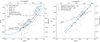 |
Fig. 1 Left panel: [C/O]–[O/H] correlation based on Garnett et al. (1995) (dot-dashed black), Nicholls et al. (2017) (dashed black), and Amarsi et al. (2019) observations, the latter using the best-fit relations of Sharda et al. (2023b,a) (solid blue). The dotted black line shows the case when C/H scales linearly with O/H. The filled blue circles show the [C/O]−[O/H] pairs for which we performed the PDR modeling. The corresponding values for a linear relation between C/H and O/H are shown as empty blue circles. The observational data of Berg et al. (2016, 2019); Ravindranath et al. (2020); Izotov et al. (2023) are shown for comparison, including star-forming galaxies with abundances measured via recombination lines (Esteban et al. 2002, 2009, 2014; Pilyugin & Thuan 2005; García-Rojas & Esteban 2007; López-Sánchez et al. 2007). The secondary y-axis shows the log10(C/O) abundance ratio. Right panel: |

2.3 Column density distributions
For the input AV, obs–PDFs (hereafter, AV-PDFs) in PDFCHEM, a collection of log-norm probability density functions was considered for which we varied the median (m) and the width (σPDF). This variation in turn determined the values of the mean visual extinction  and the mode
  , with the latter being the value of AV, obs at which the distribution function peaks. We refer to Bisbas et al. (2019) and their Eqs. (2)–(5) for the definition of these values and their connection to the probability function. Table 2 presents a summary of the input AV-PDFs properties, and Fig. 2 represents them graphically. These distributions represent different types of ISM clouds that are dense enough to form stars under typical MW conditions. For example, Goodman et al. (2009) reported a mean AV, obs ∼3 mag in clouds based on their study of the Perseus star-forming region, whose extent is ∼20 pc. Kainulainen et al. (2009) reported various mean AV ∼1–3 mag of star-forming and non-star-forming clouds with sizes of ∼4 pc. Higher AV, obs values (∼6 mag) were found by Froebrich & Rowles (2010) in nearby giant molecular clouds, while a more extended study considering 195 nearby clouds was performed by Abreu-Vicente et al. (2015). This study covered cloud sizes of ≲ 15 pc with a mean Av, obs ∼3−20 mag. This range matches the range we considered. Similar values were reported by Schneider et al. (2016); Spilker et al. (2021); Ma et al. (2022), and others (see also Bisbas et al. 2019, 2023, for further discussion).
For all metallicities we explored, the above suite of AV-PDFs was treated as the total column density distribution (Ntot-PDFs) at solar metallicity. This assumption (also taken previously in Bisbas et al. 2019, 2021, 2023, 2024) implies that the density distribution and the size of the clouds are always kept the same at all metallicities. This shows the trends of the dependence of the conversion factors on the environmental parameters of the ISM better. Under this assumption, the choice of m = 15 was taken to ensure that considerable amounts of H2-rich gas were always present in low metallicities and under most of the environmental parameters of the ISM we explored. For a given AV-PDF at any metallicity, we therefore used the same AV, eff – nH relation in terms of density distribution and effective size of the cloud at solar metallicity, but we integrated up to different depths (locations inside the cloud) depending on the metallicity.
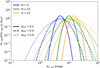 |
Fig. 2 Input observed AV-PDFs used in PDFCHEM. We used three different medians (m = 5 blue line, m = 10 green line, and m = 15 orange line) and three different widths (σPDF = 0.2 solid lines, σPDF = 0.4 dashed lines, and σPDF = 0.6 dotted lines) that corresponded to different values of the mean |

2.4 Calculation of conversion factors
We estimated the XC* conversion factor of the coolant (where C* represents C or CO) using the following expression:
![Mathematical equation: $X_{\mathrm{C} *}=\frac{\left\langle\mathrm{N}\left(\mathrm{H}_{2}\right)\right\rangle}{\left\langle W_{\mathrm{C} *}\right\rangle}\left[\mathrm{cm}^{-2} /\left(\mathrm{K}\, \mathrm{km} \mathrm{s}^{-1}\right)\right],$](/articles/aa/full_html/2025/05/aa54067-25/aa54067-25-eq14.png) (3)
(3)
where ⟨N(H2)⟩ is the average H2 column density of the AV, obs-PDF and ⟨WC*⟩ the average velocity-integrated emission of the coolant. We estimated ⟨N(H2)⟩ using the following expression:
 (4)
(4)
where N(H2)i is the H2 column density of the ith computational element of the AV,eff − nH relation (see Bisbas et al. 2019, 2023).
For each PDR model and depth point, we calculated the radiation temperature (TC*) of the coolant by solving the radiative transfer equation as explained by Bisbas et al. (2017a, 2023). To calculate the optical depth, and consequently, the radiation temperature, we used the level populations of the coolants resulting from each 3D-PDR model under LTE conditions and using the LVG escape-probability approximation (see Bisbas et al. 2012, for full details).
The average velocity-integrated emission, ⟨WC*⟩, was estimated by calculating TC*, multiplied by the line width, Δ V,
 (5)
(5)
where
![Mathematical equation: $\Delta V=2 \sqrt{2 \ln 2} \sqrt{\frac{k_{\mathrm{B}} T_{\text {gas}}}{m_{\text {mol}}}+v_{\text {Turb}}^{2}}[\mathrm{~km} / \mathrm{s}].$](/articles/aa/full_html/2025/05/aa54067-25/aa54067-25-eq17.png) (6)
(6)
In all models we present, we assumed a macroturbulent velocity dispersion of vTurb = 1.5 km/s. For instance, for the CO molecule and for a gas with Tgas = 10 K, the above expression gives a ΔV ∼3.5 km s−1, which agrees with observations (e.g. Heyer & Dame 2015; Rice et al. 2016).
3 Results
3.1 Effect of the X-factors on the environmental parameters of the ISM
Figures 3 and 4 show logarithmic grid maps4 of the X-factors for two representative AV-PDFs, namely with m = 5 and 15 mag and with σPDF = 0.4. In general, the HI-to-H2 transition decreases in the ζCR−χ/χ0 space as [O/H] decrease, so in low metallicities the distribution remains molecular for weak values of FUV intensities and cosmic-ray ionization rates. For [O/H] ≥ 0, the distributions remain molecular for most of the ζCR−χ/χ0 range. The particular set of m = 5 distributions is mainly atomic for [O/H] = −1.0. As expected, we found that log-normal AV-PDFs with m < 5 mag contain hardly any molecular gas in low-metallicity ISM conditions.
We can determine the dependence of each X-factor on ζCR and χ/χ0 and the corresponding trends based on Figs. 3 and 4. The XCI-factor illustrated in the top row of both figures shows almost no dependence on the intensity of the FUV radiation field for [O/H] ≥ 0, but rather on the cosmic-ray ionization rate, because the high  value shields the distribution from the interaction with FUV photons. We find that XCI decreases with increasing ζCR as a result of the effect of cosmic-ray-induced destruction of CO, which leads to an increase in the C abundance (Bisbas et al. 2015, 2017b), and consequently, to the [CI] (1–0) emission (Bisbas et al. 2021). Because [C/O] and
  both decrease with [O/H], as illustrated in Fig. 1, the FUV radiation is able to penetrate further, reaches higher column densities, and consequently, higher H-nucleus number densities. This causes the XCI-factor to become more responsive to the change in the χ/χ0 value. For solar neighborhood metallicities and above ([O/H] ≳ −0.2) and for a low and fixed ζCR, XCI decreases with increasing intensity of the FUV radiation field, as we illustrate in Fig. 5. This occurs because the [CI] emission increases faster than the slower decrease in N(H2).
The bottom row of Figs. 3 and 4 shows the dependence of XCO on ζCR and χ/χ0 for the two representative AV-PDFs. As with the XCI, the CO conversion factor depends more strongly on ζCR than on the FUV intensity for [O/H] ≥ 0 and even for [O/H] = −0.2 in high-density clouds. For more diffuse clouds than explored here, it is expected that at these metallicities, XCO inevitably depends on the χ/χ0 value (see e.g. Bisbas et al. 2023). In contrast to the trends observed in XCI, the XCO-factor behaves differently when ζCR increases for a fixed χ/χ0. XCO fluctuates irregularly as the cosmic-ray ionization rate increases. The discrepancy in the XCO values, especially in the m = 15 mag distribution (Fig. 4) for [O/H] ≳ −0.2, is very small. This implies that for clouds with a high column density like this, the XCO-factor depends weakly on the environmental parameters of the ISM. For lower metallicities, the conversion factor described above mainly depends on the intensity of the FUV radiation even for the higher column density distribution. It is expected that cosmic-rays only affect low-metallicity environments for the very high density condensations that cannot be penetrated by FUV photons.
Figure 5 shows the behavior of the CO and C X-factors as a function of the FUV intensity for a fixed ζCR = 10−17 s−1 cosmic-ray ionization rate (top panel) and as a function of the ζCR for a fixed χ/χ0 = 1 FUV intensity (bottom panel). Both panels refer to [O/H] = 0. The top panel shows that the FUV intensity does not affect the XCO-factor, which agrees remarkably well with the MW average (XCO ∼2 × 1020 cm−2(K km s−1)−1 Bolatto et al. 2013), regardless of the AV-PDF. However, as the χ/χ0 increases, the XCI decreases since the abundance of C and the gas temperature increase, which leads to a brighter emission of the [CI] (1–0) line. The increase in the cosmic-ray ionization rate for fixed χ/χ0 as illustrated in the bottom panel causes a nonlinear variation in the XCO-factor. Depending on m, the XCO-factor slightly decreases for ζCR = 10−16 s−1 before a local maximum forms at ζCR ≃ 10−14 s−1 (see also Bell et al. 2006). This nonlinear behavior is connected with an increase in the gas temperature at high column densities through cosmic-ray heating, which changes the CO formation pathway via the OH channel (Bisbas et al. 2017b). On the other hand, the XCI factor shows a more linear and decreasing trend.
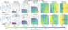 |
Fig. 3 Logarithmic grid maps (in the common logarithmic space of log10) showing the X-conversion factors using the [CI] (1–0) (top) and the CO (1−0) (bottom), defined as the ratio of the PDF-averaged H2 column density to the PDF-averaged brightness temperature multiplied by the line width. These panels show results of the AV-PDF of m = 5 mag and σPDF = 0.4, corresponding to |

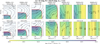 |
Fig. 4 As in Fig. 3, but for an AV-PDF distribution of m = 15 mag and σPDF = 0.4, corresponding to an average AV of |

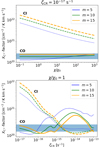 |
Fig. 5 Conversion factors at [O/H] = 0 for a fixed ζCR = 10−17 s−1 (top panel) and for a fixed χ/χ0 = 1 (bottom panel). The AV-PDF widths are σPDF = 0.4. The blue lines correspond to m = 5, the green lines to m = 10, and the orange lines to m = 15 mag. The solid lines correspond to XCO, and the dashed lines show XCI. The shaded blue stripe represents the average MW value. |
3.2 General behavior of the X-factors
Figure 6 shows the change in the XCO and XCI factors as a function of metallicity. For all assumed AV distributions, we considered the PDF-averaged value of the conversion factor of each coolant. In these calculations, we excluded very low and very high values of the FUV intensities (χ/χ0 < 0.5. and χ/χ0 > 102) and high values of the cosmic-ray ionization rates (ζCR>10−15 s−1) because these values represent more specific systems. We also note that we assumed equal weights to calculate the averages of all combinations, including the environmental parameters of the ISM and the input AV-PDF.
The results of our models are shown as solid blue lines in both panels of Fig. 6. The dashed black lines refer to the best-fit values of the PDFCHEM results for [C/O] < 0, which are given by the expressions for the CO-to-H2 conversion factor
 (7)
(7)
and for the [CI]-to-H2 conversion factor
 (8)
(8)
where Z = 12 + log10(O/H). Our results broadly agree with observations, as described below. For comparison, we also plot the corresponding XCO and XCI factors for the linear decrease versus metallicity (marked as [C/O] = 0) as dotted gray lines. For a linear decrease in the C and O abundances and the dust-to-gas mass ratio, Eqs. (7) and (8) take the form log10 XCO,lin = −1.869 Z+36.681 and log10 XCI,lin = −1.011 Z + 29.554, respectively. The [C/O] < 0 ratios tend to increase the XCO factor more toward low metallicities than for [C/O] = 0, which agrees better with the observations. Similarly, negative [C/O] tends to shift the XCI factor upward in the metallicity regime we explored. Overall, the two X factors show a declining trend with increasing [O/H], which leads to sub-MW values for a metal-rich ISM ([O/H] > 0). This agrees with several observations and models of the metal-poor ISM that used CO as a molecular gas tracer (e.g. Genzel et al. 2012; Schruba et al. 2012; Bolatto et al. 2013; Amorín et al. 2016; Tacconi et al. 2018) or [CI] (e.g. Accurso et al. 2017; Madden et al. 2020; Bisbas et al. 2021).
In Fig. 6, we also show a collection of observational data for comparison. These include the average XCO factor value of our Galaxy (Bolatto et al. 2013), the SMC and LMC (Israel 1997)5, observations from the Local Group of galaxies (Leroy et al. 2011), the WLM galaxy (Elmegreen et al. 2013) which is a dwarf irregular galaxy with metallicity Z = 0.13 Z⊙ observed in CO (3–2), the very metal poor (Z ∼0.07 Z⊙) galaxy Sextans A (Shi et al. 2015), as well as the dwarf galaxies DDO-70, DDO-53 and DDO-50 (Shi et al. 2016). All these works estimated the H2 column density based on the dust emission, while Elmegreen et al. (2013) further assumed a CO (3−2)/CO (1−0) = 0.8 ratio to convert the observed CO (3–2) into CO (1–0). Furthermore, we plot two best-fit relations from the literature. The first one concerns the Genzel et al. (2012) fit resulting from a sample of high-redshift (z ≥ 1) star-forming galaxies of the so-called main-sequence in which the H2 gas mass has been estimated from the star formation rate using the Kennicutt-Schmidt relation (Kennicutt 1998). The second one concerns the Madden et al. (2020) fit resulting from the Dwarf Galaxy Survey (DGS; Madden et al. 2013) who used Cloudy models to estimate the H2 gas mass from [CII] and CO (1−0) observations.
The curves in the figure that result from the PDFCHEM algorithm (Eqs. (7) and (8)) consider the total emission and total H2 column density of each distribution without adopting any limit for the observational sensitivities. In reality, we expect that the faintest part of the CO emission is not captured by radio telescopes, which leaves a portion of H2-rich gas as undetected based on this line and makes it CO-dark, as we also discuss below. To accommodate this, we plot the CO-to-H2 conversion factor when this observational sensitivity was taken into account. In particular, we adopted a minimum brightness temperature of TCO (1–0) = 0.1 K, which is representative of the typical sensitivity limit in observations (e.g. Nieten et al. 2006; Smith et al. 2014; Leroy et al. 2016; Tokuda et al. 2021; Luo et al. 2024), and we also calculated the H2 column density for TCO(1−0) ≥ 0.1 K. We then calculated both the PDF-averaged brightness temperature of the line and the PDF-averaged H2 column density above this limit. Their ratio therefore represents a CO-to-H2 conversion factor that is tightly connected with the CO-bright H2 gas and omits the CO-dark component. The left panel of Fig. 6 shows that the discrepancy between the blue and cyan lines is very small for solar metallicities because the CO-dark gas fraction is very small under these conditions (see the discussion in Sect. 3.3). As the metallicity decreases, this discrepancy increases and approximately reaches two orders of magnitude for the lowest-metallicity case. This implies that at these low metallicities, the CO-bright component may account for just a few percent of the real H2 gas mass that exists in these distributions. The higher sensitivity limits tend to shift the cyan CO-to-H2 curve upward, as expected.
In the right panel of Fig. 6, the observations of Heintz & Watson (2020) are shown along with their best-fit relation. These are high-redshift observations of star-forming galaxies using gamma-ray burst and quasar absorbers to estimate the H2 column density and the [CI] luminosity. We also plot the best-fit relation of Ramambason et al. (2024) corresponding to low-metallicity dwarf galaxies from the DGS. Ramambason et al. (2024) used the statistical algorithm MULTIGRIS and the PDR code Cloudy (Ferland et al. 2017) to estimate the luminosity of [CI] through CO lines. As for the CO-to-H2 case, we also accounted for a similar observational sensitivity of T[CI](1−0) = 0.1 K. The cyan line illustrated in the right panel of Fig. 6 indicates that the [CI] (1–0) fine-structure line remains a more robust tracer of molecular gas even at very low metallicities. This line may not always arise directly from the molecular gas component, but rather from the PDR surface for typical ISM conditions for the FUV and ζCR values. For high ζCR, however, the [CI] (1–0) line originates directly from the H2 gas, as discussed in previous works (Bisbas et al. 2015, 2017b, 2021).
Although Fig. 6 shows the dependence of the conversion factors on metallicity (on average), it would be interesting to explore the individual dependence of the cosmic-ray ionization rate, the FUV intensity and the density distribution on XCO and XCI as a function of metallicity. This is discussed below.
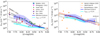 |
Fig. 6 XCO-factor (left panel) and the XCI-factor (right panel) for all models (solid blue lines). The dashed black lines illustrate the best-fit expressions (Eqs. (7) and (8) for XCo and XCI, respectively). We show in the left panel the observations of Israel (1997); Leroy et al. (2011); Elmegreen et al. (2013); Shi et al. (2015, 2016), including the average MW value (shown as the large blue star (Bolatto et al. 2013)) and the best-fit relations of Genzel et al. (2012) and Madden et al. (2020). We show in the right panel the observations of Heintz & Watson (2020) and their best-fit relation together with that of Ramambason et al. (2024). For all scattered observational data, we plot the reported error bars, which may be smaller than the symbol size. In all cases, the PDFCHEM best-fit expressions match the observations well. In both panels, the case of [C/O] = 0 is shown as the dotted gray line, which further assumes the linear relation of |

3.2.1 Dependence on the cosmic-ray ionization rate
The top row of Fig. 7 shows the change induced by the increasing ζCR parameter on the conversion factors for a FUV radiation that is fixed at χ/χ0 = 1. For ζCR ≤ 10−16 s−1, the XCO (left panel) remains approximately constant for metallicities down to 12 + log10(O/H) ≃ 8.4. For lower metallicities, the conversion factor increases and approaches the Madden et al. (2020) best-fit. At higher CR values of ζCR = 10−15 s−1, for example, the XCO factor increases, but not as strongly as with lower ζCR, because the average gas temperature increases, which causes CO (1–0) to become brighter in high-density regions (Bisbas et al. 2021) affecting the XCO value. For ζCR = 10−14 s−1, it remains approximately constant at XCO ∼1021 cm−2/K km s−1 for all metallicities. For ζCR this high and for 12 + log10(O/H) ≲ 8.1, none of the assumed AV-PDFs is H2-dominated. On the other hand, the XCI factor appears to depend more strongly on the ζCR value, although the dispersion in XCI values is far lower than that of XCO (the values on the y-axis are far lower). Interestingly, for each cosmic-ray ionization rate, the [CI]-to-H2 conversion factor remains to within a factor of ∼5 at a low metallicity, as opposed to the CO-to-H2 factor, which may change by more than two orders of magnitude. For solar metallicities, however, XCI does depend strongly on the ζCR rate. The value of the conversion factor spans approximately two orders of magnitude. This spread declines as the metallicity decreases. This is supported by the finding that for fixed χ/χ0 and ζCR, XCI does not change significantly in low-Z.
3.2.2 Dependence on the FUV intensity
The middle row of Fig. 7 shows the dependence on the strength of the FUV radiation field for a fixed ζCR = 10−17 s−1. For solar metallicities and above, the XCO factor apparently does not depend on the value of χ/χ0 for the AV-PDF we explored (see also the top panel of Fig. 5). However, as the metallicity decreases, low FUV intensities tend to return a lower CO-to-H2 conversion factor than higher FUV intensities. The reason is that as the radiation strength increases, photodissocation changes the depth point at which the transition phase of the carbon cycle (C+/C/CO) occurs, which leads to a slower build-up in the CO abundance, and thus, to a weaker CO (1–0) emission (see also Bell et al. 2006). It is interesting to note that the estimates by Israel (1997) of the XCO factor agree better with strong FUV radiation fields than with cosmic-ray ionization rates. Stronger FUV intensities than in the average MW in the diffuse ISM of the Magellanic Clouds were indeed reported (Pradhan et al. 2011; Israel & Maloney 2011). For high χ/χ0, the density distributions may also not be H2 rich because of photodissociation. On the other hand, the XCI factors shown in the right panel of the middle row do not depend as strongly on the FUV intensity for different metallicities as XCO. However, for solar metallicities (e.g., the MW), the [CI]-to-H2 factor is spread by approximately one order of magnitude; lower χ/χ0 are connected with higher XCI values. This trend appears to be reversed at low metallicities. A variation in the FUV intensities cannot reproduce the observed [CI]-to-H2 conversion factors below the best-fit functions of Heintz & Watson (2020) and Ramambason et al. (2024).
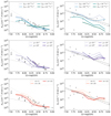 |
Fig. 7 XCO (left column) and XCI (right column) conversion factors vs. metallicity as a function of the FUV intensity (top row), the cosmic-ray ionization rate (middle row), and the density distribution (bottom row). The panels in the top row illustrate the dependence on ζCR for a fixed FUV intensity of χ/χ0 = 1. The panels in the middle row show the dependence on χ/χ0 for a fixed ζCR = 10−17 s−1. In the top and middle rows, we consider all three m and three σ values (nine distributions in total) of Table 2. The panels in the bottom row illustrate the dependence on the mean, m, of the AV-PDF for a fixed σPDF = 0.4. The bottom panels are averages for 10−17 ≤ ζCR ≤ 10−15 s−1 and 0.5 ≤ χ/χ0 ≤ 102. In all panels, the gray scatter points and the gray lines correspond to the observations and best-fit relations described in Fig. 6. |
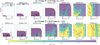 |
Fig. 8 Logarithmic grid maps as in shown in Figs. 3 and 4, but colored with respect to the logarithmic fDARK CO-dark gas fraction. The upper row shows results for the m = 5 and σPDF = 0.4 distribution, and the bottom row shows results for the m = 15 and σPDF = 0.4 distribution. |
3.2.3 Dependence on the column density distribution
In the bottom row of Fig. 7, we plot the dependence of the conversion factors on the mean (m) of the AV-PDFs. For these results, we assumed a fixed width of σPDF = 0.4, and we considered FUV intensities and cosmic-ray ionization rates in the ranges of 0.5 ≤ χ/χ0 ≤ 102 and 10−17 ≤ ζCR ≤ 10−15 s−1, respectively. The two conversion factors depend on the value of m; lower mean values produce a higher X factor in general. The SMC and LMC observations (Israel 1997) also agree with the low-density distributions. A dependence on the column density distribution might also be connected with the evolutionary stage of clouds. This relation has previously been observed in the low-metallicity dwarf galaxy NGC 6822 (Schruba et al. 2017), in which the CO-to-H2 conversion factors exceed the MW value by about 20 times. The XCI factor depends much more weakly on the column density distribution. The three-dimensional PDR models of Bisbas et al. (2021) that examined the conversion factors of a star-forming and a non-star-forming density distribution agree with this. The authors found that high-density structures tend to have a much lower XCO factor in the metal-poor ISM than low-density structures, whereas their XCI factors remained approximately constant even for supersolar metallicities.
3.3 CO-dark molecular gas fraction
As described in the Introduction, CO-dark refers to the cold H2-rich gas that is not observed in CO line emission. Essentially, a CO-dark molecular gas has two causes: i) the absence of CO molecules in molecular regions in translucent and diffuse clouds because CO self-shielding is weaker than that of H2, and ii) the sensitivity limit of telescopes that are able to detect the CO (1–0) line emission above some threshold. In the observational context, the term CO-dark refers to the second case, and the first case is better studied (if not only studied) with numerical modeling (see also discussion in Seifried et al. 2020).
We adopted the observational definition of CO-dark, that is, the H2-rich gas with a CO (1−0) brightness temperature of <0.1 K (chosen limit, as discussed above). In turn, the CO-dark gas fraction, fDARK, is defined here as the ratio of the H2 column density with a TCO(1−0) < 0.1 K to the total H2 column density of the PDR model,
 (9)
(9)
Figure 8 shows logarithmic grid maps of the fDARK ratio for the two representative AV-PDFs discussed in Sect. 3.1. In both cases (which implies that a similar result is expected for all distributions we considered), we find that the H2-rich gas becomes progressively CO-dark as [O/H] decreases and severely CO-dark for [O/H] = −1.0. Only for metallicities [O/H] ≥−0.8 and for denser (m = 15 mag) distributions is the molecular gas CO-bright, and this is the case for very low FUV intensities. As the metallicity increases toward [O/H] = 0 and above, the fraction of CO-dark gas decreases overall. As expected, for higher m values, the effect of a decreasing fDARK is stronger. In addition, for a constant [O/H], fDARK increases with increasing ζCR when ζCR ≳ 10−15 s−1 through the CR-induced destruction of CO. For lower ζCR, the CO-dark gas fraction primarily depends on the FUV intensity.
Figure 9 shows the general trends of the CO-dark gas for all AV-PDFs we considered. For each distribution, the plotted curves represent the average of the molecular region (colored partition in Fig. 8). The top panel shows that fDARK increases with decreasing [O/H]. As expected, the denser the molecular cloud (higher m), the lower fDARK for fixed [O/H] when compared to a more diffuse molecular cloud (lower m). Moreover, for fixed m, the width (σPDF) of the distribution does not change the CO-dark fraction by much. The effect of the ambient environmental parameters of the ISM (ζCR and χ/χ0) on fDARK is shown in the lower panel of Fig. 9. The standard deviation, σ(log10  ), peaks for [O/H] ∼ −0.4 to −0.2. We therefore argue that for [O/H] ∼ −0.2 (the average metallicity of the ISM in the solar neighbourhood), both ζCR and χ/χ0 play an important role when the H2 gas mass is estimated through the commonly used CO (1–0) emission line.
While a large fraction of CO-dark molecular gas exists in the low-metallicity ISM in particular, as we found above, it would be interesting to determine whether this H2 gas can be observed using the [CI] (1−0) fine-structure line instead. Figure 10 shows the change in the brightness temperature ratio of CO (1−0) and [CI] (1–0) as a function of ζCR and χ/χ0 for the two representative Av-PDFs discussed in Sect. 3.1. For metallicities close to solar (e.g., [O/H] ≳ −0.2) and above and for low cosmic-ray ionization rates (e.g. ζCR ≲ 10−15 s−1), we found that the brightness temperature of CO (1−0) is much higher than that of [CI] (1–0). The [CI] (1–0) becomes brighter for higher ζCR values, which agrees with the earlier findings of Bisbas et al. (2015, 2017b, 2021). For lower metallicities, the [CI] (1–0) line dominates, except for combinations of low ζCR ≲ 10−16 s−1 and low χ/χ0 ≲ 1. Distributions reflecting high-density or star-forming gas (e.g. m = 15) may contain small clumps of high depths in column that remain bright in CO (1−0) even for very low metallicities (Madden et al. 2020) provided that cosmic rays and the intensity of the FUV radiation are severely attenuated. The [CI] (1–0) line might therefore be a good alternative for tracing molecular gas in low-metallicity environments. The much weaker variation in the XCI conversion factor compared to XCO versus metallicity (Fig. 6) also supports this result.
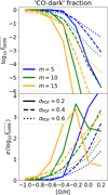 |
Fig. 9 Mean values (top) of the logarithmic X conversion factor for all AV-PDFs, and the corresponding standard deviation around the mean (bottom). Top panel: average log10 |

4 Discussion
The results of the models presented by Bisbas et al. (2024) and in this paper show that a nonlinear C/O ratio versus metallicity that leads to an α-enhanced ISM has important implications for studying metal-poor galaxies. In general, the thermal balance of the ISM strongly affects the behavior of molecular gas tracers. This effect primarily arises from the much less efficient dust-shielding in low-metallicity environments which leads to a much lower efficiency in the H2 formation. The effect is also caused by the lower C/O ratios, which affect the total gas cooling.
In low-metallicity environments, the C/O ratio is affected by the distinct stellar nucleosynthesis pathways of carbon and oxygen, which cause a differential enrichment of C and O as a function of O/H. This leads to changes in the efficiency of molecular gas tracers. In particular, we find that as CO becomes much less abundant in low-metallicity environments through the reduced self-shielding and lower formation efficiency, the [CI] emission may become more prominent because it traces the regions in which CO formation is less efficient. Since the nonlinear C/O ratio and the dust-to-gas ratios affect the thermal balance of the ISM, it is expected that the physical conditions of the ISM influencing the efficiency of the star formation will be different in low-metallicity galaxies. This affects the initial mass function (e.g. Marks et al. 2012; Bate 2019; Sharda & Krumholz 2022; Tanvir & Krumholz 2024).
However, for metallicities higher than solar, we find that the conversion factors become very stable against most of the environmental parameters of the ISM we explored. For [O/H] = 0.2, our models showed that the FUV radiation field and the column-density distribution of the cloud (represented by the considered AV-PDFs) do not affect the CO-to-H2 or the [CI]-to-H2 conversion factors. Only when a higher cosmic-ray ionization rate is applied does the X factors of both these tracers change. Notably, for higher ζCR values, the XCO increases while XCI decreases. This is connected to the efficient destruction of CO by cosmic rays, which leads to a more extended [CI]-bright molecular gas (Bisbas et al. 2015, 2021). For these supersolar metallicities, our models show that effects connected to different C/O and dust-to-gas mass ratios from the commonly used linear assumptions cease to be important.
Our models assumed the density function arising from the AV,eff – nH relation and used this for all thermochemical models presented here. This relation was found to operate in small-scale (parsec) and large-scale (kiloparsec) structures (e.g. Glover et al. 2010; Van Loo et al. 2013; Safranek-Shrader et al. 2017; Seifried et al. 2017; Hu et al. 2021). In our models, we assumed that the density distribution does not change with metallicity. This assumption was made in previous similar works (e.g. Bisbas et al. 2019, 2023, 2024). However, in low-metallicity environments, the weaker shielding by dust in combination with the lower abundances of metals changes the thermal balance, and this affects the overall density distribution. Very few models exploring this AV,eff – nH relation and its connection to metallicity variations have been reported. The hydrodynamical models of Hu et al. (2021) offer this insight and reported a correlation of the form  , where α increases slightly as the metallicity decreases. This indicates a systematic shift in the relation at lower metallicities that is caused by changes in dust shielding and cloud structure. In general, Hu et al. (2021) did not report a strong dependence of this relation on metallicity. This confirms our results.
The CO-dark fraction of molecular gas increases strongly at low metallicities. In addition, diffuse clouds contain higher CO-dark fractions than denser/star-forming clouds even at solar metallicities. These trends agree with previous observational works. For instance, earlier Herschel studies by Langer et al. (2014) on individual clouds within MW found that the fraction of CO-dark H2 gas decreases with increasing total column density, and that clouds in the outer/metal-poor regions of our Galaxy have a greater fraction of CO-dark H2. This is consistent with our results. In line with a larger fraction of CO-dark H2 gas in low-metallicity gas, Balashev et al. (2017) reported results obtained for a high-redshift (z ≃ 2.786) damped Ly α absorption system, which was found to contain large amounts of H2 gas, but poor CO-bright gas, as evident from the very high conversion factor of 1−3 × 10³ times the Galactic CO-to-H2. More recently, Chevance et al. (2020) reported a large fraction of CO-dark gas in the massive star-forming region 30 Doradus in the LMC, which has half the solar metallicity.
Our finding that the XCO factor exhibits a higher dispersion with decreasing metallicity is consistent with observational studies. For instance, Leroy et al. (2011) and Schruba et al. (2012) reported significant variations in the XCO factor in different low-metallicity environments, with values ranging from a few times to several hundred times the Galactic average. These variations were attributed to the complex relation between metallicity, dust shielding, and the local ISM conditions. Similarly, Madden et al. (2020) observed a wide range of XCo values in low-metallicity dwarf galaxies, which further supports the idea that the CO-to-H2 conversion factor becomes increasingly uncertain in metal-poor environments. In line with this trend of a larger dispersion with decreasing metallicity are the observations reported by Elmegreen et al. (2013) and Shi et al. (2015, 2016), as illustrated in the left panel of Fig. 6.
The [CI]-to-H2 factor appears to be a reliable choice for molecular gas studies in low-metallicity environments. Our models showed that the XCI factor varies little with changes in the ISM parameters, such as the FUV intensity and the cosmic-ray ionization rate. This variability was also found to be weaker than the corresponding variability for the XCO factor. While both XCI and XCO increase as metallicity decreases, the CO-to-H2 conversion factor exhibits a much steeper rise. This makes it more difficult to interpret in extreme environments with low [O/H]. In contrast, the response of XCI to these changes is more gradual and predictable. A significant fraction of molecular gas at low metallicities cannot be effectively traced by the CO emission (Bolatto et al. 2013; Chevance et al. 2020; Madden et al. 2020). We found that the [CI] (1–0) line is closely linked to the H2-rich and CO-deficit regions. It is therefore better suited for the detection of this molecular gas component.
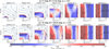 |
Fig. 10 Logarithmic grid maps showing the ratio of CO (1−0) and [CI] (1−0) brightness temperatures. The color bar corresponds to the logarithm of this ratio. Positive values (red) indicate a stronger CO (1–0) brightness temperature, and negative values (blue) show a stronger [CI] (1−0) brightness temperature. The upper row corresponds to the m = 5 and σPDF = 0.4, and the bottom row shows the m = 15 and σPDF distribution. |
5 Conclusions
We continued the efforts of Bisbas et al. (2024) in studying the impact of α-enhanced ISM environments on observables. In particular, we studied the impact of negative [C/O] ratios and observation-driven dust-to-gas ratios versus metallicity in the CO-to-H2 and the [CI]-to-H2 conversion factors. Our study used the recently developed algorithm PDFCHEM, which estimates the average PDR quantities from entire distributions of column densities using a set of precalculated 1D PDR models following the AV,eff – nH relation modeled with 3D-PDR. We also considered a set of AV-PDF functions that interact with a wide range of FUV intensities and cosmic-ray ionization rates. We covered many different combinations that represent quiescent and extreme conditions.
Our study found that the CO-to-H2 conversion factor strongly depends on metallicity and that it increases significantly with decreasing metallicity. For environments with [O/H] = −1.0, XCO is ≳ 1000× higher than the average Galactic value for [C/O] < 0 conditions, whereas it is ≲ 300 × for [C/O] = 0. This highlights the significant sensitivity of the C/O and dust-to-gas ratios for studies of the metal-poor ISM. The trend of increasing XCO is consistent with the reduced CO formation efficiency in low-metallicity conditions. However, the CO-to-H2 factor is also sensitive to the environmental parameters of the ISM, in particular, the cosmic-ray ionization rate. This can lead to highly nonlinear variations.
The [CI]-to-H2 conversion factor shows a moderate dependence on metallicity compared to XCO, and it decreases with increasing metallicity, but within a narrower range. XCI is less sensitive to variations in the FUV radiation field at low metallicities. This makes it a more reliable tracer of molecular gas in these environments. This reliability highlights its potential as an alternative to CO for the molecular gas mass estimation in metal-poor galaxies.
The fraction of CO-dark molecular gas increases significantly in the low-metallicity ISM, with values exceeding 90% for [O/H] = −1.0. This reflects the inefficiency of CO self-shielding in these environments, where H2 can form and persist without detectable CO emission. The CO-dark fraction is strongly affected by the FUV intensity and cosmic-ray ionization rate, in particular, at intermediate metallicities ([O/H] ≃ −0.4). These findings underline the challenges of accurately estimating the molecular gas content using CO emission alone in metal-poor systems.
For estimating the molecular mass content in galaxies with metallicities in the range of −1 < [O/H] < 0.2 examined here, we recommend the use of Eqs. (7) and (8) for the CO-to-H2 and [CI]-to-H2 ratio, respectively. However, we note that in very metal-poor conditions, the conversion factors especially for XCO depend strongly on the local environmental conditions of the ISM. The variations may reach more than an order of magnitude. It is therefore imperative to examine each different system carefully and individually.
Acknowledgements
The authors thank the anonymous referee for their comments that help improve the clarity of our work. This work is supported by the National Key Research & Development (R&D) Programme of China (Grant No. 2023YFA1608204). This work is supported by the Leading Innovation and Entrepreneurship Team of Zhejiang Province of China (Grant No. 2023R01008). Part of this work was supported by the German Deutsche Forschungsgemeinschaft, DFG project number Ts 17/2-1. Z.-Y.Z. acknowledges the support of the National Natural Science Foundation of China (NSFC; Grant Nos. 12173016 and 12041305), and the Programme for Innovative Talents, Enterpreneur in Jiangsu. Y.Z. is grateful for support from the National Natural Science Foundation of China (NSFC) under grant No. 12173079. T.T. gratefully acknowledges the Collaborative Research Center 1601 (SFB 1601 subproject A6) funded by the Deutsche Forschungsgemeinschaft (DFG, German Research Foundation) – 500700252. D.L. acknowledges support from the National Natural Science Foundation of China (NSFC) Grant No. 11988101. D.L. is a New Cornerstone Investigator.
Appendix A Density-weighted gas temperatures
Figure A.1 shows the average, density-weighted, gas temperature of three AV-PDFs with m = 15 and σPDF of 0.2 (blue line), 0.4 (green line) and 0.6 (orange line). In all cases ζCR = 10−16 s−1 and χ/χ0 = 1. The gas temperature increases with decreasing [O/H], which impacts the shape of CO SLEDs. For the aforementioned distribution, we find that ⟨Tgas⟩ is ∼10 K for [O/H] ∼ −0.2 to 0.2, while for [O/H] ≲ −0.8 it can reach ∼20−22 K. This enhances the CO emission and particularly the high-J transitions which can eventually lead to elevated CO SLEDs.
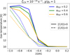 |
Fig. A.1 Density-weighted gas temperatures for the AV-PDF distributions with m = 15 and σPDF = 0.2 (blue), 0.4 (green) and 0.6 (orange). In all cases, ζCR = 10−16 s−1 and χ/χ0 = 1. Solid lines represent the [C/O] < 0 case, whereas dashed lines the [C/O] = 0 case. |
With dashed lines we plot the linear case ([C/O] = 0 and  respectively). For metallicities [O/H] ≳ −0.4, the average gas temperature does not show an appreciable difference. However, for lower metallicities the linear relation predicts a lower gas temperature, primarily due to the higher dust-to-gas ratios which attenuate the FUV radiation decreasing, consequently, the amount of photoelectric heating. However, for very metal-poor gas (e.g. [O/H] ∼ −1.0), the gas temperatures predicted by both bases of [C/O] are quite similar.
Appendix B Linear assumption of [C/O] and  versus [O/H]
Table B.1 shows the abundances of carbon, oxygen and the gas-to-dust ratio (normalized to the solar value) when a linear decrease versus metallicity is assumed. Figure B.1 (similar to Fig. 7) shows the dependence of both X-factors on the cosmic-ray ionization rate, the FUV intensity and the AV-PDF versus metallicity for that assumption.
Under the linear assumption, the XCO-factor shows a less pronounced increase with decreasing metallicity compared to the nonlinear case, particularly at low metallicities ([O/H] ≲ −0.6). This is because the linear decrease in [C/O] and \mathcal{D} results in less extreme variations in dust shielding and CO formation efficiency. However, XCO still exhibits significant sensitivity to ζCR and χ/χ0, with higher cosmic-ray ionization rates leading to nonlinear fluctuations in XCO due to changes in gas temperature and CO formation pathways.

For XCI, the linear assumption results in a more gradual decline with increasing metallicity compared to the nonlinear case. The [CI]-to-H2 factor remains relatively stable across a wide range of metallicities, with less sensitivity to ζCR and χ/χ0 than XCO. This concludes that [CI] (1–0) is a more reliable tracer of molecular gas in low-metallicity environments, even under simplified assumptions about the ISM composition.
The linear assumption, while useful for comparison, underestimates the complexity of the ISM environment and its impact on molecular gas tracers.
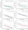 |
Fig. B.1 As in Fig. 7 for the “linear” conditions of C/O ratio ([C/O] = 0) and the dust-to-gas ratio |

References
- Abreu-Vicente, J., Kainulainen, J., Stutz, A., Henning, T., & Beuther, H., 2015, A&A, 581, A74 [CrossRef] [EDP Sciences] [Google Scholar]
- Accurso, G., Saintonge, A., Bisbas, T. G., & Viti, S., 2017, MNRAS, 464, 3315 [NASA ADS] [CrossRef] [Google Scholar]
- Aller, L. H., & Greenstein, J. L., 1960, ApJS, 5, 139 [Google Scholar]
- Amarsi, A. M., Nissen, P. E., Asplund, M., Lind, K., & Barklem, P. S., 2019, A&A, 622, L4 [NASA ADS] [CrossRef] [EDP Sciences] [Google Scholar]
- Amorín, R., Muñoz-Tuñón, C., Aguerri, J. A. L., & Planesas, P., 2016, A&A, 588, A23 [NASA ADS] [CrossRef] [EDP Sciences] [Google Scholar]
- Asano, R. S., Takeuchi, T. T., Hirashita, H., & Inoue, A. K. 2013a, Earth Planets Space, 65, 213 [NASA ADS] [CrossRef] [Google Scholar]
- Asano, R. S., Takeuchi, T. T., Hirashita, H., & Nozawa, T., 2013b, MNRAS, 432, 637 [NASA ADS] [CrossRef] [Google Scholar]
- Asplund, M., Grevesse, N., Sauval, A. J., & Scott, P., 2009, ARA&A, 47, 481 [NASA ADS] [CrossRef] [Google Scholar]
- Balashev, S. A., Noterdaeme, P., Rahmani, H., et al. 2017, MNRAS, 470, 2890 [CrossRef] [Google Scholar]
- Bate, M. R., 2019, MNRAS, 484, 2341 [NASA ADS] [CrossRef] [Google Scholar]
- Bell, T. A., Roueff, E., Viti, S., & Williams, D. A., 2006, MNRAS, 371, 1865 [NASA ADS] [CrossRef] [Google Scholar]
- Bell, T. A., Viti, S., & Williams, D. A., 2007, MNRAS, 378, 983 [NASA ADS] [CrossRef] [Google Scholar]
- Berg, D. A., Skillman, E. D., Henry, R. B. C., Erb, D. K., & Carigi, L., 2016, ApJ, 827, 126 [NASA ADS] [CrossRef] [Google Scholar]
- Berg, D. A., Erb, D. K., Henry, R. B. C., Skillman, E. D., & McQuinn, K. B. W., 2019, ApJ, 874, 93 [NASA ADS] [CrossRef] [Google Scholar]
- Bialy, S., Sternberg, A., Lee, M.-Y., Le Petit, F., & Roueff, E., 2015, ApJ, 809, 122 [NASA ADS] [CrossRef] [Google Scholar]
- Bigiel, F., de Looze, I., Krabbe, A., et al. 2020, ApJ, 903, 30 [CrossRef] [Google Scholar]
- Bisbas, T. G., Bell, T. A., Viti, S., Yates, J., & Barlow, M. J., 2012, MNRAS, 427, 2100 [NASA ADS] [CrossRef] [Google Scholar]
- Bisbas, T. G., Papadopoulos, P. P., & Viti, S., 2015, ApJ, 803, 37 [NASA ADS] [CrossRef] [Google Scholar]
- Bisbas, T. G., Tanaka, K. E. I., Tan, J. C., Wu, B., & Nakamura, F. 2017a, ApJ, 850, 23 [NASA ADS] [CrossRef] [Google Scholar]
- Bisbas, T. G., van Dishoeck, E. F., Papadopoulos, P. P., et al. 2017b, ApJ, 839, 90 [Google Scholar]
- Bisbas, T. G., Schruba, A., & van Dishoeck, E. F., 2019, MNRAS, 485, 3097 [NASA ADS] [Google Scholar]
- Bisbas, T. G., Tan, J. C., & Tanaka, K. E. I., 2021, MNRAS, 502, 2701 [CrossRef] [Google Scholar]
- Bisbas, T. G., van Dishoeck, E. F., Hu, C.-Y., & Schruba, A. 2023, MNRAS, 519, 729 [Google Scholar]
- Bisbas, T. G., Zhang, Z.-Y., Gjergo, E., et al. 2024, MNRAS, 527, 8886 [Google Scholar]
- Bolatto, A. D., Wolfire, M., & Leroy, A. K., 2013, ARA&A, 51, 207 [CrossRef] [Google Scholar]
- Borchert, E. M. A., Walch, S., Seifried, D., et al. 2022, MNRAS, 510, 753 [Google Scholar]
- Chevance, M., Madden, S. C., Fischer, C., et al. 2020, MNRAS, 494, 5279 [Google Scholar]
- Choban, C. R., Kereš, D., Sandstrom, K. M., et al. 2024, MNRAS, 529, 2356 [CrossRef] [Google Scholar]
- Cooke, R. J., Pettini, M., & Steidel, C. C., 2017, MNRAS, 467, 802 [NASA ADS] [Google Scholar]
- Crocker, A. F., Pellegrini, E., Smith, J. D. T., et al. 2019, ApJ, 887, 105 [NASA ADS] [CrossRef] [Google Scholar]
- Dabrowski, I., 1984, Can. J. Phys., 62, 1639 [NASA ADS] [CrossRef] [Google Scholar]
- Dame, T. M., Hartmann, D., & Thaddeus, P., 2001, ApJ, 547, 792 [Google Scholar]
- Draine, B. T., 1978, ApJS, 36, 595 [Google Scholar]
- Dufour, R. J., 1984, in IAU Symposium, 108, Structure and Evolution of the Magellanic Clouds, eds. S. van den Bergh & K. S. D. de Boer, 353 [Google Scholar]
- Dunne, L., Maddox, S. J., Vlahakis, C., & Gomez, H. L., 2021, MNRAS, 501, 2573 [NASA ADS] [CrossRef] [Google Scholar]
- Dunne, L., Maddox, S. J., Papadopoulos, P. P., Ivison, R. J., & Gomez, H. L., 2022, MNRAS, 517, 962 [NASA ADS] [CrossRef] [Google Scholar]
- Elmegreen, B. G., Rubio, M., Hunter, D. A., et al. 2013, Nature, 495, 487 [NASA ADS] [CrossRef] [Google Scholar]
- Esteban, C., Peimbert, M., Torres-Peimbert, S., & Rodríguez, M., 2002, ApJ, 581, 241 [NASA ADS] [CrossRef] [Google Scholar]
- Esteban, C., Bresolin, F., Peimbert, M., et al. 2009, ApJ, 700, 654 [NASA ADS] [CrossRef] [Google Scholar]
- Esteban, C., García-Rojas, J., Carigi, L., et al. 2014, MNRAS, 443, 624 [NASA ADS] [CrossRef] [Google Scholar]
- Ferland, G. J., Chatzikos, M., Guzmán, F., et al. 2017, Rev. Mexicana Astron. Astrofis., 53, 385 [Google Scholar]
- Froebrich, D., & Rowles, J., 2010, MNRAS, 406, 1350 [NASA ADS] [Google Scholar]
- Gaches, B. A. L., Offner, S. S. R., & Bisbas, T. G., 2019, ApJ, 883, 190 [NASA ADS] [CrossRef] [Google Scholar]
- Galametz, M., Madden, S. C., Galliano, F., et al. 2011, A&A, 532, A56 [NASA ADS] [CrossRef] [EDP Sciences] [Google Scholar]
- Galliano, F., Nersesian, A., Bianchi, S., et al. 2021, A&A, 649, A18 [EDP Sciences] [Google Scholar]
- García-Rojas, J., & Esteban, C., 2007, ApJ, 670, 457 [CrossRef] [Google Scholar]
- Garnett, D. R., Skillman, E. D., Dufour, R. J., et al. 1995, ApJ, 443, 64 [Google Scholar]
- Genzel, R., Tacconi, L. J., Combes, F., et al. 2012, ApJ, 746, 69 [Google Scholar]
- Giveon, U., Sternberg, A., Lutz, D., Feuchtgruber, H., & Pauldrach, A. W. A., 2002, ApJ, 566, 880 [NASA ADS] [CrossRef] [Google Scholar]
- Glover, S. C. O., & Clark, P. C., 2016, MNRAS, 456, 3596 [Google Scholar]
- Glover, S. C. O., Federrath, C., Mac Low, M. M., & Klessen, R. S., 2010, MNRAS, 404, 2 [Google Scholar]
- Glover, S. C. O., Clark, P. C., Micic, M., & Molina, F., 2015, MNRAS, 448, 1607 [NASA ADS] [CrossRef] [Google Scholar]
- Gong, M., Ostriker, E. C., & Kim, C.-G., 2018, ApJ, 858, 16 [Google Scholar]
- Gong, M., Ostriker, E. C., Kim, C.-G., & Kim, J.-G., 2020, ApJ, 903, 142 [CrossRef] [Google Scholar]
- Goodman, A. A., Pineda, J. E., & Schnee, S. L., 2009, ApJ, 692, 91 [Google Scholar]
- Harrington, K. C., Weiss, A., Yun, M. S., et al. 2021, ApJ, 908, 95 [NASA ADS] [CrossRef] [Google Scholar]
- Heintz, K. E., & Watson, D., 2020, ApJ, 889, L7 [Google Scholar]
- Herrera-Camus, R., Fisher, D. B., Bolatto, A. D., et al. 2012, ApJ, 752, 112 [NASA ADS] [CrossRef] [Google Scholar]
- Heyer, M., & Dame, T. M., 2015, ARA&A, 53, 583 [Google Scholar]
- Hollenbach, D. J., & Tielens, A. G. G. M., 1999, Rev. Mod. Phys., 71, 173 [Google Scholar]
- Hu, C.-Y., Sternberg, A., & van Dishoeck, E. F. 2021, ApJ, 920, 44 [NASA ADS] [CrossRef] [Google Scholar]
- Hu, C.-Y., Schruba, A., Sternberg, A., & van Dishoeck, E. F. 2022, ApJ, 931, 28 [NASA ADS] [CrossRef] [Google Scholar]
- Hunt, L. K., García-Burillo, S., Casasola, V., et al. 2015, A&A, 583, A114 [NASA ADS] [CrossRef] [EDP Sciences] [Google Scholar]
- Hunt, L. K., Belfiore, F., Lelli, F., et al. 2023, A&A, 675, A64 [NASA ADS] [CrossRef] [EDP Sciences] [Google Scholar]
- Hunter, D. A., Elmegreen, B. G., & Madden, S. C., 2024, ARA&A, 62, 113 [NASA ADS] [CrossRef] [Google Scholar]
- Israel, F. P., 1997, A&A, 328, 471 [NASA ADS] [Google Scholar]
- Israel, F. P., & Maloney, P. R., 2011, A&A, 531, A19 [NASA ADS] [CrossRef] [EDP Sciences] [Google Scholar]
- Izotov, Y. I., Schaerer, D., Worseck, G., et al. 2023, MNRAS, 522, 1228 [NASA ADS] [CrossRef] [Google Scholar]
- Jiao, Q., Zhao, Y., Zhu, M., et al. 2017, ApJ, 840, L18 [Google Scholar]
- Jiao, Q., Zhao, Y., Lu, N., et al. 2019, ApJ, 880, 133 [Google Scholar]
- Jiao, Q., Gao, Y., & Zhao, Y., 2021, MNRAS, 504, 2360 [NASA ADS] [CrossRef] [Google Scholar]
- Kainulainen, J., Beuther, H., Henning, T., & Plume, R., 2009, A&A, 508, L35 [NASA ADS] [CrossRef] [EDP Sciences] [Google Scholar]
- Kennicutt, Jr., R. C. 1998, ApJ, 498, 541 [Google Scholar]
- Komugi, S., Inaba, M., & Shindou, T., 2023, PASJ, 75, 1337 [Google Scholar]
- Konstantopoulou, C., De Cia, A., Ledoux, C., et al. 2024, A&A, 681, A64 [NASA ADS] [CrossRef] [EDP Sciences] [Google Scholar]
- Lada, E. A., & Blitz, L., 1988, ApJ, 326, L69 [Google Scholar]
- Langer, W. D., Velusamy, T., Pineda, J. L., Willacy, K., & Goldsmith, P. F., 2014, A&A, 561, A122 [NASA ADS] [CrossRef] [EDP Sciences] [Google Scholar]
- Lelli, F., Zhang, Z.-Y., Bisbas, T. G., et al. 2023, A&A, 672, A106 [NASA ADS] [CrossRef] [EDP Sciences] [Google Scholar]
- Leroy, A. K., Bolatto, A., Gordon, K., et al. 2011, ApJ, 737, 12 [Google Scholar]
- Leroy, A. K., Hughes, A., Schruba, A., et al. 2016, ApJ, 831, 16 [Google Scholar]
- Lo, N., Cunningham, M. R., Jones, P. A., et al. 2014, ApJ, 797, L17 [NASA ADS] [CrossRef] [Google Scholar]
- López-Sánchez, Á. R., Esteban, C., García-Rojas, J., Peimbert, M., & Rodríguez, M. 2007, ApJ, 656, 168 [CrossRef] [Google Scholar]
- Luo, G., Li, D., Tang, N., et al. 2020, ApJ, 889, L4 [NASA ADS] [CrossRef] [Google Scholar]
- Luo, G., Li, D., Zhang, Z.-Y., et al. 2024, A&A, 685, L12 [NASA ADS] [CrossRef] [EDP Sciences] [Google Scholar]
- Ma, Y., Wang, H., Zhang, M., et al. 2022, ApJS, 262, 16 [NASA ADS] [CrossRef] [Google Scholar]
- Madden, S. C., Rémy-Ruyer, A., Galametz, M., et al. 2013, PASP, 125, 600 [NASA ADS] [CrossRef] [Google Scholar]
- Madden, S. C., Cormier, D., Hony, S., et al. 2020, A&A, 643, A141 [NASA ADS] [CrossRef] [EDP Sciences] [Google Scholar]
- Magdis, G. E., Daddi, E., Elbaz, D., et al. 2011, ApJ, 740, L15 [NASA ADS] [CrossRef] [Google Scholar]
- Magdis, G. E., Daddi, E., Béthermin, M., et al. 2012, ApJ, 760, 6 [NASA ADS] [CrossRef] [Google Scholar]
- Maiolino, R., & Mannucci, F., 2019, A&A Rev., 27, 3 [NASA ADS] [CrossRef] [Google Scholar]
- Marks, M., Kroupa, P., Dabringhausen, J., & Pawlowski, M. S., 2012, MNRAS, 422, 2246 [NASA ADS] [CrossRef] [Google Scholar]
- McElroy, D., Walsh, C., Markwick, A. J., et al. 2013, A&A, 550, A36 [NASA ADS] [CrossRef] [EDP Sciences] [Google Scholar]
- McKee, C. F., & Ostriker, E. C., 2007, ARA&A, 45, 565 [Google Scholar]
- Michiyama, T., Ueda, J., Tadaki, K.-i., et al. 2020, ApJ, 897, L19 [NASA ADS] [CrossRef] [Google Scholar]
- Michiyama, T., Saito, T., Tadaki, K.-i., et al. 2021, ApJS, 257, 28 [NASA ADS] [CrossRef] [Google Scholar]
- Nicholls, D. C., Sutherland, R. S., Dopita, M. A., Kewley, L. J., & Groves, B. A., 2017, MNRAS, 466, 4403 [Google Scholar]
- Nieten, C., Neininger, N., Guélin, M., et al. 2006, A&A, 453, 459 [CrossRef] [EDP Sciences] [Google Scholar]
- Offner, S. S. R., Bisbas, T. G., Bell, T. A., & Viti, S., 2014, MNRAS, 440, L81 [NASA ADS] [CrossRef] [Google Scholar]
- Pagel, B. E. J., 2009, Nucleosynthesis and Chemical Evolution of Galaxies (Cambridge, UK: Cambridge University Press) [Google Scholar]
- Papadopoulos, P. P., Thi, W. F., & Viti, S., 2004, MNRAS, 351, 147 [NASA ADS] [CrossRef] [Google Scholar]
- Papadopoulos, P. P., Bisbas, T. G., & Zhang, Z.-Y., 2018, MNRAS, 478, 1716 [NASA ADS] [CrossRef] [Google Scholar]
- Pilyugin, L. S., & Thuan, T. X., 2005, ApJ, 631, 231 [CrossRef] [Google Scholar]
- Popping, G., & Péroux, C., 2022, MNRAS, 513, 1531 [CrossRef] [Google Scholar]
- Pradhan, A. C., Murthy, J., & Pathak, A., 2011, ApJ, 743, 80 [Google Scholar]
- Ramambason, L., Lebouteiller, V., Madden, S. C., et al. 2024, A&A, 681, A14 [NASA ADS] [CrossRef] [EDP Sciences] [Google Scholar]
- Ravindranath, S., Monroe, T., Jaskot, A., Ferguson, H. C., & Tumlinson, J., 2020, ApJ, 896, 170 [NASA ADS] [CrossRef] [Google Scholar]
- Rémy-Ruyer, A., Madden, S. C., Galliano, F., et al. 2013, A&A, 557, A95 [Google Scholar]
- Rémy-Ruyer, A., Madden, S. C., Galliano, F., et al. 2014, A&A, 563, A31 [Google Scholar]
- Rice, T. S., Goodman, A. A., Bergin, E. A., Beaumont, C., & Dame, T. M., 2016, ApJ, 822, 52 [Google Scholar]
- Röllig, M., Abel, N. P., Bell, T., et al. 2007, A&A, 467, 187 [Google Scholar]
- Romano, D., 2022, A&A Rev., 30, 7 [NASA ADS] [CrossRef] [Google Scholar]
- Safranek-Shrader, C., Krumholz, M. R., Kim, C.-G., et al. 2017, MNRAS, 465, 885 [NASA ADS] [CrossRef] [Google Scholar]
- Sandstrom, K. M., Leroy, A. K., Walter, F., et al. 2013, ApJ, 777, 5 [Google Scholar]
- Savitzky, A., & Golay, M. J. E., 1964, Analyt. Chem., 36, 1627 [NASA ADS] [CrossRef] [Google Scholar]
- Schneider, N., Bontemps, S., Motte, F., et al. 2016, A&A, 587, A74 [NASA ADS] [CrossRef] [EDP Sciences] [Google Scholar]
- Schruba, A., Leroy, A. K., Walter, F., et al. 2012, AJ, 143, 138 [NASA ADS] [CrossRef] [Google Scholar]
- Schruba, A., Leroy, A. K., Kruijssen, J. M. D., et al. 2017, ApJ, 835, 278 [NASA ADS] [CrossRef] [Google Scholar]
- Scoville, N., Sheth, K., Aussel, H., et al. 2016, ApJ, 820, 83 [Google Scholar]
- Seifried, D., Walch, S., Girichidis, P., et al. 2017, MNRAS, 472, 4797 [NASA ADS] [CrossRef] [Google Scholar]
- Seifried, D., Haid, S., Walch, S., Borchert, E. M. A., & Bisbas, T. G., 2020, MNRAS, 492, 1465 [NASA ADS] [CrossRef] [Google Scholar]
- Shapley, A. E., Cullen, F., Dunlop, J. S., et al. 2020, ApJ, 903, L16 [NASA ADS] [CrossRef] [Google Scholar]
- Sharda, P., & Krumholz, M. R., 2022, MNRAS, 509, 1959 [Google Scholar]
- Sharda, P., Amarsi, A. M., Grasha, K., et al. 2023a, MNRAS, 525, 3316 [Google Scholar]
- Sharda, P., Amarsi, A. M., Grasha, K., et al. 2023b, MNRAS, 518, 3985 [Google Scholar]
- Shi, Y., Wang, J., Zhang, Z.-Y., et al. 2015, ApJ, 804, L11 [CrossRef] [Google Scholar]
- Shi, Y., Wang, J., Zhang, Z.-Y., et al. 2016, Nat. Commun., 7, 13789 [NASA ADS] [CrossRef] [Google Scholar]
- Skalidis, R., Goldsmith, P. F., Hopkins, P. F., & Ponnada, S. B., 2024, A&A, 682, A161 [NASA ADS] [CrossRef] [EDP Sciences] [Google Scholar]
- Smith, R. J., Glover, S. C. O., Clark, P. C., Klessen, R. S., & Springel, V., 2014, MNRAS, 441, 1628 [NASA ADS] [CrossRef] [Google Scholar]
- Sofia, U. J., Lauroesch, J. T., Meyer, D. M., & Cartledge, S. I. B., 2004, ApJ, 605, 272 [NASA ADS] [CrossRef] [Google Scholar]
- Spilker, A., Kainulainen, J., & Orkisz, J., 2021, A&A, 653, A63 [NASA ADS] [CrossRef] [EDP Sciences] [Google Scholar]
- Sternberg, A., Le Petit, F., Roueff, E., & Le Bourlot, J., 2014, ApJ, 790, 10 [CrossRef] [Google Scholar]
- Strong, A. W., & Mattox, J. R., 1996, A&A, 308, L21 [NASA ADS] [Google Scholar]
- Szűcs, L., Glover, S. C. O., & Klessen, R. S., 2016, MNRAS, 460, 82 [CrossRef] [Google Scholar]
- Tacconi, L. J., Genzel, R., Saintonge, A., et al. 2018, ApJ, 853, 179 [Google Scholar]
- Tanvir, T. S., & Krumholz, M. R., 2024, MNRAS, 527, 7306 [Google Scholar]
- Tielens, A. G. G. M., 2005, The Physics and Chemistry of the Interstellar Medium (Cambridge, UK: Cambridge University Press) [Google Scholar]
- Tielens, A. G. G. M., & Hollenbach, D., 1985, ApJ, 291, 722 [Google Scholar]
- Tokuda, K., Kondo, H., Ohno, T., et al. 2021, ApJ, 922, 171 [NASA ADS] [CrossRef] [Google Scholar]
- Trainor, R. F., Strom, A. L., Steidel, C. C., & Rudie, G. C., 2016, ApJ, 832, 171 [NASA ADS] [CrossRef] [Google Scholar]
- Triani, D. P., Sinha, M., Croton, D. J., Pacifici, C., & Dwek, E., 2020, MNRAS, 493, 2490 [NASA ADS] [CrossRef] [Google Scholar]
- van Dishoeck, E. F., 1990, in Astronomical Society of the Pacific Conference Series, 12, The Evolution of the Interstellar Medium, ed. L. Blitz, 207 [Google Scholar]
- van Dishoeck, E. F., 1992, in Astrochemistry of Cosmic Phenomena, 150, ed. P. D. Singh, 143 [Google Scholar]
- Van Loo, S., Butler, M. J., & Tan, J. C., 2013, ApJ, 764, 36 [NASA ADS] [CrossRef] [Google Scholar]
- Wolfire, M. G., Vallini, L., & Chevance, M., 2022, ARA&A, 60, 247 [NASA ADS] [CrossRef] [Google Scholar]
- Yasuda, A., Kuno, N., Sorai, K., et al. 2023, PASJ, 75, 743 [NASA ADS] [CrossRef] [Google Scholar]
- Zanella, A., Daddi, E., Magdis, G., et al. 2018, MNRAS, 481, 1976 [Google Scholar]
- Zhao, Y., Liu, J., Zhang, Z.-Y., & Bisbas, T. G., 2024, ApJ, 977, 46 [Google Scholar]
- Zhukovska, S., 2014, A&A, 562, A76 [NASA ADS] [CrossRef] [EDP Sciences] [Google Scholar]
The square bracket notation [A/B] represents the logarithmic ratio of the number of atoms of element A to element B, normalized to a reference value (here the Sun):
![Mathematical equation: $[\mathrm{A} / \mathrm{B}]=\log _{10}\left(\frac{N_{\mathrm{A}}}{N_{\mathrm{B}}}\right)-\log _{10}\left(\frac{N_{\mathrm{A}}}{N_{\mathrm{B}}}\right)_{\odot},$](/articles/aa/full_html/2025/05/aa54067-25/aa54067-25-eq34.png) (1)
(1)
(Aller & Greenstein 1960; Pagel 2009). The values [O/H] = 0 and [C/O] = 0 represent Solar abundances of O and C with 12 + log10(O/H) = 8.69 and 12 + log10(C/H) = 8.43, respectively (Asplund et al. 2009).
In Figs. 3, 4, and 10, we apply a two-dimensional Savitzky & Golay (1964) filter to reduce the numerical noise, using the algorithm available at https://github.com/espdev/sgolay2
There are two values of XCO for NGC 4499 in their Tables 3 and 4. We have used the data of Table 4 with the error scaled accordingly.
All Tables
All Figures
|
Fig. 1 Left panel: [C/O]–[O/H] correlation based on Garnett et al. (1995) (dot-dashed black), Nicholls et al. (2017) (dashed black), and Amarsi et al. (2019) observations, the latter using the best-fit relations of Sharda et al. (2023b,a) (solid blue). The dotted black line shows the case when C/H scales linearly with O/H. The filled blue circles show the [C/O]−[O/H] pairs for which we performed the PDR modeling. The corresponding values for a linear relation between C/H and O/H are shown as empty blue circles. The observational data of Berg et al. (2016, 2019); Ravindranath et al. (2020); Izotov et al. (2023) are shown for comparison, including star-forming galaxies with abundances measured via recombination lines (Esteban et al. 2002, 2009, 2014; Pilyugin & Thuan 2005; García-Rojas & Esteban 2007; López-Sánchez et al. 2007). The secondary y-axis shows the log10(C/O) abundance ratio. Right panel: |
| In the text | |
|
Fig. 2 Input observed AV-PDFs used in PDFCHEM. We used three different medians (m = 5 blue line, m = 10 green line, and m = 15 orange line) and three different widths (σPDF = 0.2 solid lines, σPDF = 0.4 dashed lines, and σPDF = 0.6 dotted lines) that corresponded to different values of the mean |
| In the text | |
|
Fig. 3 Logarithmic grid maps (in the common logarithmic space of log10) showing the X-conversion factors using the [CI] (1–0) (top) and the CO (1−0) (bottom), defined as the ratio of the PDF-averaged H2 column density to the PDF-averaged brightness temperature multiplied by the line width. These panels show results of the AV-PDF of m = 5 mag and σPDF = 0.4, corresponding to |
| In the text | |
|
Fig. 4 As in Fig. 3, but for an AV-PDF distribution of m = 15 mag and σPDF = 0.4, corresponding to an average AV of |
| In the text | |
|
Fig. 5 Conversion factors at [O/H] = 0 for a fixed ζCR = 10−17 s−1 (top panel) and for a fixed χ/χ0 = 1 (bottom panel). The AV-PDF widths are σPDF = 0.4. The blue lines correspond to m = 5, the green lines to m = 10, and the orange lines to m = 15 mag. The solid lines correspond to XCO, and the dashed lines show XCI. The shaded blue stripe represents the average MW value. |
| In the text | |
|
Fig. 6 XCO-factor (left panel) and the XCI-factor (right panel) for all models (solid blue lines). The dashed black lines illustrate the best-fit expressions (Eqs. (7) and (8) for XCo and XCI, respectively). We show in the left panel the observations of Israel (1997); Leroy et al. (2011); Elmegreen et al. (2013); Shi et al. (2015, 2016), including the average MW value (shown as the large blue star (Bolatto et al. 2013)) and the best-fit relations of Genzel et al. (2012) and Madden et al. (2020). We show in the right panel the observations of Heintz & Watson (2020) and their best-fit relation together with that of Ramambason et al. (2024). For all scattered observational data, we plot the reported error bars, which may be smaller than the symbol size. In all cases, the PDFCHEM best-fit expressions match the observations well. In both panels, the case of [C/O] = 0 is shown as the dotted gray line, which further assumes the linear relation of |
| In the text | |
|
Fig. 7 XCO (left column) and XCI (right column) conversion factors vs. metallicity as a function of the FUV intensity (top row), the cosmic-ray ionization rate (middle row), and the density distribution (bottom row). The panels in the top row illustrate the dependence on ζCR for a fixed FUV intensity of χ/χ0 = 1. The panels in the middle row show the dependence on χ/χ0 for a fixed ζCR = 10−17 s−1. In the top and middle rows, we consider all three m and three σ values (nine distributions in total) of Table 2. The panels in the bottom row illustrate the dependence on the mean, m, of the AV-PDF for a fixed σPDF = 0.4. The bottom panels are averages for 10−17 ≤ ζCR ≤ 10−15 s−1 and 0.5 ≤ χ/χ0 ≤ 102. In all panels, the gray scatter points and the gray lines correspond to the observations and best-fit relations described in Fig. 6. |
| In the text | |
|
Fig. 8 Logarithmic grid maps as in shown in Figs. 3 and 4, but colored with respect to the logarithmic fDARK CO-dark gas fraction. The upper row shows results for the m = 5 and σPDF = 0.4 distribution, and the bottom row shows results for the m = 15 and σPDF = 0.4 distribution. |
| In the text | |
|
Fig. 9 Mean values (top) of the logarithmic X conversion factor for all AV-PDFs, and the corresponding standard deviation around the mean (bottom). Top panel: average log10 |
| In the text | |
|
Fig. 10 Logarithmic grid maps showing the ratio of CO (1−0) and [CI] (1−0) brightness temperatures. The color bar corresponds to the logarithm of this ratio. Positive values (red) indicate a stronger CO (1–0) brightness temperature, and negative values (blue) show a stronger [CI] (1−0) brightness temperature. The upper row corresponds to the m = 5 and σPDF = 0.4, and the bottom row shows the m = 15 and σPDF distribution. |
| In the text | |
|
Fig. A.1 Density-weighted gas temperatures for the AV-PDF distributions with m = 15 and σPDF = 0.2 (blue), 0.4 (green) and 0.6 (orange). In all cases, ζCR = 10−16 s−1 and χ/χ0 = 1. Solid lines represent the [C/O] < 0 case, whereas dashed lines the [C/O] = 0 case. |
| In the text | |
|
Fig. B.1 As in Fig. 7 for the “linear” conditions of C/O ratio ([C/O] = 0) and the dust-to-gas ratio |
| In the text | |
Current usage metrics show cumulative count of Article Views (full-text article views including HTML views, PDF and ePub downloads, according to the available data) and Abstracts Views on Vision4Press platform.
Data correspond to usage on the plateform after 2015. The current usage metrics is available 48-96 hours after online publication and is updated daily on week days.
Initial download of the metrics may take a while.