| Issue |
A&A
Volume 643, November 2020
|
|
|---|---|---|
| Article Number | A141 | |
| Number of page(s) | 21 | |
| Section | Extragalactic astronomy | |
| DOI | https://doi.org/10.1051/0004-6361/202038860 | |
| Published online | 17 November 2020 | |
Tracing the total molecular gas in galaxies: [CII] and the CO-dark gas⋆
1
AIM, CEA, CNRS, Université Paris-Saclay, Université Paris Diderot, Sorbonne Paris Cité, 91191 Gif-sur-Yvette, France
e-mail: suzanne.madden@cea.fr
2
Institut für Theoretische Astrophysik, Zentrum für Astronomie der Universität Heidelberg, Albert-Ueberle Str. 2, 69120 Heidelberg, Germany
3
University of Cincinnati, Clermont College, 4200 Clermont College Drive, Batavia, OH 45103, USA
4
Sterrenkundig Observatorium, Ghent University, Krijgslaan 281 S9, 9000 Gent, Belgium
5
Department of Physics and Astronomy, University College London, Gower Street, London WC1E 6BT, UK
6
Astronomisches Rechen-Institut, Zentrum für Astronomie der Universität Heidelberg, Mönchhofstrasse 12-14, 69120 Heidelberg, Germany
7
LERMA, Observatoire de Paris, PSL Research University, CNRS, Sorbonne Université, 75014 Paris, France
8
Korea Astronomy and Space Science Institute, 776 Daedeokdae-ro, 34055 Daejeon, Republic of Korea
Received:
6
July
2020
Accepted:
14
August
2020
Context. Molecular gas is a necessary fuel for star formation. The CO (1−0) transition is often used to deduce the total molecular hydrogen but is challenging to detect in low-metallicity galaxies in spite of the star formation taking place. In contrast, the [C II]λ158 μm is relatively bright, highlighting a potentially important reservoir of H2 that is not traced by CO (1−0) but is residing in the C+-emitting regions.
Aims. Here we aim to explore a method to quantify the total H2 mass (MH2) in galaxies and to decipher what parameters control the CO-dark reservoir.
Methods. We present Cloudy grids of density, radiation field, and metallicity in terms of observed quantities, such as [O I], [C I], CO (1−0), [C II], LTIR, and the total MH2. We provide recipes based on these models to derive total MH2 mass estimates from observations. We apply the models to the Herschel Dwarf Galaxy Survey, extracting the total MH2 for each galaxy, and compare this to the H2 determined from the observed CO (1−0) line. This allows us to quantify the reservoir of H2 that is CO-dark and traced by the [C II]λ158 μm.
Results. We demonstrate that while the H2 traced by CO (1−0) can be negligible, the [C II]λ158 μm can trace the total H2. We find 70 to 100% of the total H2 mass is not traced by CO (1−0) in the dwarf galaxies, but is well-traced by [C II]λ158 μm. The CO-dark gas mass fraction correlates with the observed L[C II]/LCO(1−0) ratio. A conversion factor for [C II]λ158 μm to total H2 and a new CO-to-total-MH2 conversion factor as a function of metallicity are presented.
Conclusions. While low-metallicity galaxies may have a feeble molecular reservoir as surmised from CO observations, the presence of an important reservoir of molecular gas that is not detected by CO can exist. We suggest a general recipe to quantify the total mass of H2 in galaxies, taking into account the CO and [C II] observations. Accounting for this CO-dark H2 gas, we find that the star-forming dwarf galaxies now fall on the Schmidt–Kennicutt relation. Their star-forming efficiency is rather normal because the reservoir from which they form stars is now more massive when introducing the [C II] measures of the total H2 compared to the small amount of H2 in the CO-emitting region.
Key words: photon-dominated region / galaxies: ISM / galaxies: dwarf / HII regions / infrared: ISM
Data in Fig. 6 are only available at the CDS via anonymous ftp to cdsarc.u-strasbg.fr (130.79.128.5) or via http://cdsarc.u-strasbg.fr/viz-bin/cat/J/A+A/643/A141
© S. C. Madden et al. 2020
 Open Access article, published by EDP Sciences, under the terms of the Creative Commons Attribution License (https://creativecommons.org/licenses/by/4.0), which permits unrestricted use, distribution, and reproduction in any medium, provided the original work is properly cited.
1. Introduction
Our usual view of star formation posits the molecular gas reservoir as a necessary ingredient, the most abundant molecule being H2. This concept is borne out through testimonies of the first stages of star formation associated with and within molecular clouds and numerous observational studies showing the observed correlation of star formation with indirect tracers of H2 reflected in the Schmidt–Kennicutt relationship (e.g. Kennicutt 1998; Kennicutt et al. 2007; Bigiel et al. 2008; Leroy et al. 2008, 2013; Genzel et al. 2012; Kennicutt & Evans 2012; Kumari et al. 2020). However, directly witnessing the emission of H2 associated with the bulk of the molecular clouds is not feasible. Indeed, H2 emits weakly in molecular clouds due to the lack of a permanent dipole moment and the high temperatures necessary to excite even the lowest rotational transitions (the two lowest transitions have upper level energies, hν/k, of 510 K and 1015 K). Therefore, H2 observations can only directly trace a relatively small budget (15% to 30%) of warmer (∼100 K) molecular gas in galaxies (e.g. Roussel et al. 2007; Togi & Smith 2016), but not the larger reservoir of cold (∼10−20 K) molecular gas normally associated with star formation.
In spite of four orders of magnitude lower abundance of CO compared to H2, most studies rely on CO rotational transitions to quantify the properties of the H2 reservoir in galaxies. The low excitation temperature of CO (1−0) (∼5 K), along with its low critical density (ncrit) for collisional excitation (∼103 cm−3), make it a relatively strong, easily excited millimetre (mm) emission line to trace the cold gas in star-forming galaxies. Studies within our Galaxy long ago established a convenient recipe to convert the observed CO (1−0) emission line to H2 gas mass, that is, the XCO conversion factor (see Bolatto et al. 2013, for historical and theoretical development). Likewise, galaxies in our local universe have also routinely relied on CO observations to quantify the H2 reservoir (e.g. Leroy et al. 2011; Bigiel et al. 2011; Schruba et al. 2012; Cormier et al. 2014, 2016; Saintonge et al. 2017). CO is also commonly used to probe the H2 and star formation activity in the high-z (z ∼ 1−2) universe (e.g. Tacconi et al. 2010, 2018, 2020; Daddi et al. 2010, 2015; Combes et al. 2013; Carilli & Walter 2013; Walter et al. 2014; Genzel et al. 2015; Kamenetzky et al. 2017; Pavesi et al. 2018), although for higher-z sources, higher J CO lines may become more readily available, but relating these to the bulk of the H2 mass is less straightforward (e.g. Papadopoulos et al. 2008; Gallerani et al. 2014; Kamenetzky et al. 2018; Vallini et al. 2018; Dessauges-Zavadsky et al. 2020). Well-known caveats can hamper accurate total H2 gas mass determination in galaxies based on observed CO emission only, including those associated with assumptions on CO excitation properties, dynamical effects related to XCO, presence of ensembles of molecular clouds along the lines of sight in galaxies and low filling factor and abundance of CO compared to H2, as in low-metallicity environments (e.g. Maloney & Black 1988; Glover & Mac Low 2011; Shetty et al. 2011; Narayanan et al. 2012; Pineda et al. 2014; Clark & Glover 2015; Bisbas et al. 2017).
However, CO can fail altogether to trace the full H2 reservoir, particularly in low-metallicity galaxies. Lower dust abundance allows the far-ultraviolet (FUV) photons to permeate deeper into molecular clouds compared to more metal-rich clouds, photodissociating CO molecules, leaving a larger C+-emitting envelope surrounding a small CO core. H2, on the other hand, photodissociates via absorption of Lyman-Werner band photons, which, for moderate AV, can become optically thick, allowing H2 to become self-shielded from photodissociation (e.g. Gnedin & Draine 2014), leaving a potentially significant reservoir of H2 existing outside of the CO-emitting core, within the C+-emitting envelope (Fig. 1). The presence of this CO-dark molecular gas (e.g. Papadopoulos et al. 2002; Röllig et al. 2006; Wolfire et al. 2010; Glover & Clark 2012a) necessitates other means to trace this molecular gas reservoir that is not probed by CO. The total H2 mass is therefore the CO-dark gas mass plus the H2 within the CO-emitting core. Efficient star formation in this CO-dark gas has been shown theoretically to be possible (e.g. Krumholz & Gnedin 2011; Glover & Clark 2012b).
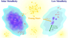 |
Fig. 1. Comparison of a solar metallicity (metal-rich) molecular cloud and a low-metallicity cloud impacted by the UV photons of nearby star clusters. The decrease in dust shielding in the case of the low-metallicity cloud leads to further photodissociation of the molecular gas, leaving a layer of self-shielded H2 outside of the small CO-emitting cores. This CO-dark H2 can, in principle, be traced by [C II] or [C I]. |
More recently, observations of the submillimetre (submm) transitions of [C I] have been used to trace the total H2 gas mass in galaxies at high and low-z, especially due to the advent of the spectroscopic capabilities of SPIRE (Griffin et al. 2010) on the Herschel Space Observatory (Pilbratt et al. 2010) and with ALMA (Popping et al. 2017; Andreani et al. 2018; Jiao et al. 2019; Nesvadba et al. 2019; Bourne et al. 2019; Valentino et al. 2020; Dessauges-Zavadsky et al. 2020), while theory and simulations (Papadopoulos et al. 2004; Offner et al. 2014; Tomassetti et al. 2014; Glover & Clark 2016; Bothwell et al. 2017; Li et al. 2018; Heintz & Watson 2020) deem [C I] to be a viable tracer of CO-dark H2. Likewise, ALMA has opened the window to numerous detections of [C II]λ158 μm in the high-z universe, making [C II], which is more luminous than [C I], a popular tracer of total H2 in galaxies (e.g. Zanella et al. 2018; Bethermin et al. 2020; Schaerer et al. 2020; Tacconi et al. 2020). Dust mass estimates via monochromatic or full spectral energy distribution (SED) studies have also been used to quantify the total H2 gas mass in the nearby and distant universe (e.g. da Cunha et al. 2013; Groves et al. 2015, more background on the different approaches to uncover CO-dark gas is presented in the following Sect. 2).
Local and global environmental effects, including star formation properties and metallicity, require consideration as well when choosing the approach to relate total gas mass to star formation. Low-metallicity environments present well-known issues in pinning down the molecular gas mass. Detecting CO in dwarf galaxies has been notoriously difficult (e.g. Leroy et al. 2009, 2012; Schruba et al. 2012; Cormier et al. 2014; Hunt et al. 2015; Grossi et al. 2016; Amorín et al. 2016, and references within), leaving us with uncertainties in quantifying the total molecular gas reservoir.
Star-forming dwarf galaxies often have super star clusters which have stellar surface densities greatly in excess of normal H II regions and OB associations. Thus, the dearth of detectable CO raises questions concerning the fueling of such active star formation. Possible explanations may include the following: (1) CO is not a reliable tracer of the total molecular gas reservoir; (2) there is a real under-abundance of molecular gas indicative of an excessively high star formation efficiency; (3) H2 has been mostly consumed by star formation; (4) H2 has been completely dissociated in the aftermath of star formation; and (5) HI is the important reservoir to host star formation.
These issues compound the difficulty in understanding the processes of both local and global star formation in low-metallicity environments. Developing reliable calibrators for the total MH2 in low-metallicity galaxies is a necessary step to be able to refine recipes for converting gas into stars under early universe conditions and thus further our understanding of how galaxies evolve. Understanding the detailed physics and chemistry of the structure and properties of the gas that fuels star formation can help us to discriminate strategies for accurate methods to get to the bulk of the molecular gas in galaxies.
Since carbon is one of the most abundant species in galaxies, its predominantly molecular form, CO, and its neutral and ionised forms, C0 and C+, play important roles in the cooling of the interstellar medium (ISM) of galaxies. The locations of the transitions from ionised carbon, to neutral carbon, to CO, which are within the photodissociation region (PDR)-molecular cloud structure, depend on numerous local physical conditions, including the FUV radiation field strength (G0)1, hydrogen number density (nH), gas abundances, metallicity (Z), dust properties, and so on. Low-metallicity star-forming environments seem to harbour unusual PDR properties compared to their dustier counterparts, with notably bright [C II]λ158 μm emission compared to the often faint CO (1−0) emission, characteristics that can be attributed to the lower dust abundance along with the star formation activity and clumpy ISM (e.g. Cormier et al. 2014; Chevance et al. 2016; Madden & Cormier 2019).
In this study, we determine a basic strategy to quantify the total H2 mass in galaxies and estimate the CO-dark molecular gas mass existing outside the CO-emitting core, for a range of Z, nH, and G0. We start with the models of Cormier et al. (2015, 2019), which were generated using the spectral synthesis code Cloudy (Ferland et al. 2017) to self-consistently model the mid-infrared (MIR) and far-infrared (FIR) fine structure cooling lines and the total infrared luminosity (LTIR) from Spitzer and Herschel. This approach allows us to constrain the photoionisation and PDR region properties, quantifying the density and incident radiation field on the illuminated face of the PDR, G0. These models exploit the fact that there is a physical continuity from the PDR envelope, where the molecular gas is predominantly CO-dark, into the CO-emitting molecular cloud. This dark gas reservoir can be primarily traced by the [C II]λ158 μm line while the L[C II]/LCO(1−0) can constrain the depth of the molecular cloud and the L[C II]/LTIR and L[C II]/L[O I] constrain the G0 and density at the illuminated face of the PDR (discussed in Sect. 5.2). With this study, we determine a conversion factor to pin down the total H2, which will make use of the observed [C II], [O I], CO (1−0), and LTIR. Application of the models to the star-forming low-metallicity galaxies of the Herschel Dwarf Galaxy Survey (DGS; Madden et al. 2013), using the observed [C II] and CO (1−0) observations, allows us to extract the total H2 mass and determine the fraction of the total H2 reservoir that is not traced by CO observations as a function of metallicity and other galactic parameters.
This paper is organised as follows. In Sect. 2 we review the studies that have focused on uncovering the CO-dark reservoir in galaxies. The environments of the dwarf galaxies in the DGS are briefly summarised in Sect. 3. In Sect. 4 we introduce the observational context and the motivations of this study by comparing the L[C II]/LCO(1−0) and L[C II]/LFIR2 of the full sample of the DGS to other more metal-rich galaxies from the literature. In Sect. 5 we present Cloudy model grids and discuss the effects of G0, nH, and metallicity. In this section we walk through the steps for using the models in order to understand the mass budget of the carbon-bearing species in the PDRs and to obtain the total H2. In Sect. 6 we apply the models to the particular case of II Zw 40 observations, as an example. Section 7 discusses the model results applied to the DGS targets. In this section we extract the total H2 for these galaxies and discuss the implication of the CO-dark gas reservoirs. We provide recipes to estimate the CO-dark H2 and the total H2 gas reservoir from [C II]. Possible caveats and limitations are noted in Sect. 8 and the results are summarised in Sect. 9.
2. CO dark gas studies
Three decades ago, the FIR spectroscopic window became readily accessible from the Kuiper Airborne Observatory (KAO) and the Infrared Space Observatory (ISO). First estimates of the CO-dark H2 reservoir obtained from [C II]λ158 μm observations found that 10 to 100 times more H2 was “hidden” in the C+-emitting regions in dwarf galaxies compared to that inferred from CO (1−0) alone (Poglitsch et al. 1995; Madden et al. 1997). These early estimates, for lack of access to additional complementary FIR diagnostics to carry out detailed modeling, relied on a number of assumptions that have until now limited the use of the FIR lines to robustly quantify this CO-dark molecular gas in galaxies. Recent spatially resolved studies of [CII] in Local Group galaxies using Herschel and the Stratospheric Observatory for Infrared Astronomy (SOFIA) have also confirmed a significant presence of CO-dark gas (e.g. Fahrion et al. 2017; Requena-Torres et al. 2016; Jameson et al. 2018; Lebouteiller et al. 2019; Chevance et al. 2020). Additionally, the MIR rotational transitions of H2 from Spitzer have been invoked to deduce a significant reservoir of H2 in dwarf galaxies (Togi & Smith 2016). Other molecules observed in absorption, such as OH and HCO+, have also been used as tracers of dark molecular gas in our Galaxy (Lucas & Liszt 1996; Allen et al. 2015; Xu et al. 2016; Li et al. 2018; Nguyen et al. 2018; Liszt et al. 2019). However, the need for sufficiently high sensitivity and resolution limits their use in other galaxies.
As γ rays interact with hydrogen nuclei, they can trace the total interstellar gas. Comparison of γ ray observations in our Galaxy with CO and H0 has uncovered an important reservoir of neutral dark gas that is not traced by CO or H I (Grenier et al. 2005; Ackermann et al. 2012; Hayashi et al. 2019). While γ ray emission, in principle, can be one of the most accurate methods possible to get at the total gas mass, its use to measure the total interstellar gas mass in other galaxies is limited for now because of the need for relatively high-resolution observations.
Comparison of Herschel [C II] velocity profiles to H I emission (Langer et al. 2010, 2014; Pineda et al. 2013; Tang et al. 2016) as well as observations comparing dust, CO (1−0), and H I (Planck Collaboration XIX 2011; Reach et al. 2017) confirm that this CO-dark gas reservoir can be an important component in our Galaxy, and comparable to that traced by CO (1−0) alone. Recent hydrodynamical simulations with radiative transfer and analytic theory also demonstrate the presence of this dark gas reservoir in the Galaxy that should be traceable via [C II] (Smith et al. 2014; Offner et al. 2014; Glover & Clark 2016; Nordon & Sternberg 2016; Gong et al. 2018; Franeck et al. 2018; Seifried et al. 2020) and is often associated with spiral arms in disc galaxies. While optically thick H I can, in principle, be the source of the CO-dark gas, there is no compelling evidence that it contributes significantly to the dark neutral gas (e.g. Murray et al. 2018). Therefore, we focus here on the CO-dark H2 gas and the potential of C+, in particular, to quantify the H2 reservoir.
Dust mass measurements with Planck, compared to the gas mass measurements, have uncovered a reservoir of dark gas in the Galaxy (Planck Collaboration XIX 2011; Reach et al. 2015). Dust measurements have often provided easier means, in terms of observational strategy, to quantify the full reservoir of gas mass of galaxies in the local Universe as well as distant galaxies (e.g. Magdis et al. 2011; Leroy et al. 2011; Magnelli et al. 2012; Eales et al. 2012; Bourne et al. 2013; Sandstrom et al. 2013; Groves et al. 2015; Scoville et al. 2016; Liang et al. 2018; Bertemes et al. 2018). This approach also entails its own fundamental issues (e.g. Privon et al. 2018). The derived total molecular gas mass is a difference measure of two large quantities (H I-derived atomic gas mass and dust-derived total gas mass), which can result in large uncertainties. Dust mass determination, which is commonly derived via the modelling of the SED, requires constraints that include submm observations and necessitates dust models with assumed optical properties as a function of wavelength, composition and size distribution. Subsequently, turning total dust mass into total gas mass requires assumptions on dust-to-gas mass ratios which can carry large uncertainties depending on star formation history and metallicity and can vary by orders of magnitude, as shown by statistical studies of low-metallicity galaxies (e.g. Rémy-Ruyer et al. 2014; Roman-Duval et al. 2014; Galliano et al. 2018).
One contributing factor to the difficulty in being conclusive on the relationship of gas, dust, and star formation in low-metallicity conditions, in particular, is the fact that galaxies with full MIR to submm dust and gas modelling have been limited to mostly metal-rich environments and relatively higher star formation properties due to telescope sensitivity limitations. This impediment has been ameliorated with the broad wavelength coverage and the high spatial resolution and sensitivity of Herschel, allowing access to the gas and dust properties of low-metallicity galaxies. The DGS has compiled a large observational database of 48 low-metallicity galaxies (Madden et al. 2013), motivated by the Herschel PACS (Poglitsch et al. 2010) and Herschel SPIRE 55 to 500 μm photometry and spectroscopy capabilities.
3. Dwarf Galaxy Survey: extreme properties in low-metallicity environments
The DGS targeted the most important FIR diagnostic tracers, [C II]λ158 μm, [O I]λ63 μm, [O I]λ145 μm, [O III]λ88 μm, [N III]λ57 μm, [N II]λ122 μm, and [N II]λ205 μm (Cormier et al. 2012, 2015, 2019) in a wide range of low-Z galaxies, as low as ∼1/50 Z⊙. Additionally, the DGS collected all of the FIR and submm photometry from Herschel to investigate the dust properties of star-forming dwarf galaxies. The IR SEDs exhibit distinct characteristics setting them apart from higher metallicity galaxies with different dust properties that generally exhibit overall warmer dust than normal-metallicity galaxies; for example their obvious paucity of PAH molecules and a striking non-linear drop in dust-to-gas mass ratios at lower metallicities (Z < 0.1 Z⊙; e.g. Galametz et al. 2011; Dale et al. 2012; Rémy-Ruyer et al. 2013, 2015).
[C II] usually ranks foremost amongst the PDR cooling lines in normal-metallicity galaxies, followed by the [O I]λ63 μm, with the L[C II] + [O I]/LFIR often used as a proxy of the heating efficiency of the photoelectric effect (e.g. Croxall et al. 2012; Lebouteiller et al. 2012, 2019). Cormier et al. (2015) summarised the observed FIR fine structure lines in the DGS noting that the range of L[C II] + [[O I]/LFIR of low-metallicity galaxies is higher than that for galaxies in other surveys of mostly metal-rich galaxies (e.g. Brauher et al. 2008; Croxall et al. 2012; van der Laan et al. 2015; Cigan et al. 2016; Smith et al. 2017; Lapham et al. 2017; Díaz-Santos et al. 2017), indicating relatively high photoelectric heating efficiency in the neutral gas. However, in star-forming dwarf galaxies, the [O III]λ88 μm line is the brightest FIR line, not the [C II]λ158 μm line, as noted on full-galaxy scales (e.g. Cormier et al. 2015, 2019) as well as resolved scales (Chevance et al. 2016; Jameson et al. 2018; Polles et al. 2019). In more quiescent, metal-poor galaxies, however, the [C II]λ158 μm line is brighter than the [O III]λ88 μm line (e.g. Cigan et al. 2016). The predominance of the large-scale [O III]λ88 μm line emission, which requires an ionisation energy of 35 eV, demonstrates the ease at which such hard photons can traverse the ISM on full galaxy scales in star-forming dwarf galaxies (Cormier et al. 2010, 2012, 2015; Cormier et al. 2019), highlighting the different nature and the porous structure of the ISM of low-metallicity galaxies. Since the [O III]/[C II] has been observed to also be similarly extreme in many high-z galaxies (e.g. Laporte et al. 2019; Hashimoto et al. 2019; Tamura et al. 2019; Harikane et al. 2020), the results presented here, where we focus on low-Z star-forming galaxies, may eventually be relevant to the understanding of the total molecular gas content and structure in some high-z galaxies.
4. L[C II]/LCO(1−0) in galaxies
Figure 2 shows the CO (1−0) luminosity (LCO) and [C II] luminosities (L[C II]) normalised by FIR luminosity (LFIR) for a wide variety of environments, ranging from starburst galaxies and Galactic star forming regions to less active, more quiescent “normal” galaxies, low-metallicity star-forming dwarf galaxies, and some high-metallicity galaxies as well as some high-z galaxies. This figure, initially presented by Stacey et al. (1991) and subsequently used as a star-formation activity diagnostic, indicates that most normal and star forming galaxies are observed to have L[C II]/LCO(1−0) ∼ 1000 to 4000, with the more active starburst galaxies showing approximately a factor of three higher range of L[C II]/LCO(1−0) than the more quiescent galaxies (Stacey et al. 1991, 2010; Hailey-Dunsheath et al. 2010). The more active dusty star forming environments possess widespread PDRs exposed to intense FUV and the L[C II]/LCO(1−0) depends on the strength of the UV field and the shielding of the CO molecule against photodissociation due to H2 and dust (e.g. Stacey et al. 1991, 2010; Wolfire et al. 2010; Accurso et al. 2017a).
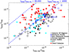 |
Fig. 2. LCO(1−0)/LFIR vs. L[C II]/LFIR observed in galaxies varying considerably in type, metallicity, and star formation properties. This is updated from Stacey et al. (1991, 2010), Madden (2000), and Hailey-Dunsheath et al. (2010) to include dwarf galaxies and more high-redshift galaxies. The dwarf galaxies are from Cormier et al. (2010, 2015) for the DGS; Grossi et al. (2016) for HeVICs dwarfs, and Smith & Madden (1997). High-redshift galaxies include those from Hailey-Dunsheath et al. (2010), Stacey et al. (2010), and Gullberg et al. (2015). The black and blue symbols are data from the original figure of Stacey et al. (1991) for Galactic star-forming regions, starburst nuclei and non-starburst nuclei, ULIRGS (Luhman et al. 2003), and normal galaxies (Malhotra et al. 2001). The dashed lines are lines of constant L[C II]/LCO(1−0). We note the location of the low-metallicity dwarf galaxies (red squares) that show extreme observed L[C II]/LCO(1−0) values. |
It has already been shown that L[C II] is somewhat enhanced relative to LFIR and more remarkably so relative to LCO in a few cases of star-forming low-metallicity galaxies compared to more metal-rich galaxies (Stacey et al. 1991; Poglitsch et al. 1995; Israel et al. 1996; Madden et al. 1997, 2011; Hunter et al. 2001; Madden & Cormier 2019). In recent, larger studies, Cormier et al. (2015, 2019) carried out detailed modelling of the DGS galaxies and compared their overall physical properties to those of more metal-rich galaxies attributing the enhanced L[C II]/LFIR to the synergy of their decreased dust abundance and active star formation. The consequence is a high ionisation parameter along with low densities resulting in a thick cloud and considerable geometric dilution of the UV radiation field. The effect over full galaxy scales is a low average ambient radiation field (G0) and relatively normal PDR gas densities (often of the order of 103 to 104 cm−3), with relatively large C+ layers. This scenario is also coherent with the L[C II]/LCO(1−0) observed in the low-metallicity galaxies.
As can be seen in Fig. 2, star-forming dwarf galaxies can reach L[C II]/LCO(1−0) ratios an order of magnitude higher or more (sometimes reaching 80 000) than their more metal-rich counterparts on galaxy-wide scales. While CO (1−0) has been difficult to detect in star-forming low-metallicity galaxies, thus shifting these galaxies well off of the Schmidt–Kennicutt relation (e.g. Cormier et al. 2014), [C II], on the other hand, has been shown to be an excellent star formation tracer over a wide range of galactic environments, including the dwarf galaxies (e.g. de Looze et al. 2011, 2014; Herrera-Camus et al. 2015). Such relatively high [C II] luminosities in star-forming dwarf galaxies harbouring little CO (1−0) may be indicative of a reservoir of CO-dark gas, which is one of the motivations for this study.
5. Using a spectral synthesis code to characterise the ISM physical conditions
The strategy of this study is to first generate model grids that will help us explore how the properties of the CO-dark gas evolve as a function of local galaxy properties, such as Z, nH, and G0, and then to determine how observational parameters can be used to pin down the mass of the CO-dark gas. We show how L[C II]/LCO(1−0) can constrain AV from the models and then the L[C II]/LTIR can narrow down the values of nH and G0 to finally quantify the total mass of H2 and hence, the mass of H2 that is not traced by CO, the CO-dark gas.
5.1. Model parameters and variations with cloud depth
We begin with the grids of Cormier et al. (2015, 2019), who use the spectral synthesis code Cloudy version 17.00 (Ferland et al. 2017), which simultaneously computes the chemical and thermal structure of H II regions physically adjacent to PDRs. The central source of the spherical geometry of the Cloudy model is the radiation extracted from Starburst99 (Leitherer et al. 2010) for a continuous starburst of 7 Myr and a total luminosity of 109 L⊙. The grids were computed by varying the initial density at the illuminated face of the H II region, nH, and the distance from the source to the edge of the illuminated H II region, the inner radius, rin. The ionisation parameter (U) is deduced in the model based on the input ionising source, rin, and nH. The models are calculated for five metallicity bins: Z = 0.05, 0.1, 0.25, 0.5, and 1.0 Z⊙3, and nH ranging from 10 to 104 cm−3. The rin values range from log(rin cm) = 20.0 to 21.3 in steps of 0.3 dex, which for the various models covers a range of U ∼ 1 to 10−5 and G0 ∼ 17 to 11481 in terms of the Habing radiation field.
A density profile that is roughly constant in the H II region and increases linearly with the total hydrogen column density (NH) beyond 1021 cm−2 is assumed (Cormier et al. 2019). To ensure that all models go deep enough into the molecular phase, regardless of the metallicity, the stopping criterion of the models is set to a CO column density of 1017.8 cm−2 (AV ∼ 10 mag). With this criterion, the optical depth of the CO(1−0) line, τCO, is greater than 1 in all models, which by our definition means that all models have transitioned in the molecular core4. For all calculations, the AV/NH ratio is computed self-consistently from the assumed grain-size distribution, grain types, and optical properties. For a more detailed description of the Cloudy models that generated the grids analysed here, see Appendix A.
Figure 3 shows the evolution of the accumulated mass, abundances, and intensities of the [C II], [C I], and CO (1−0) as a function of metallicity, density, temperature, and G0 from the H+ region into the molecular cloud. As we want to capture the properties of the H2 zone, we have defined the location of the hydrogen ionisation front and the H2 front in our calculations. As can be seen in the bottom subpanels in Fig. 3, the ionisation front is defined where H exists in the form of H+ and H0 with a ratio of 50/50; the transition between H0 and H2 is similarly where each species is 50% of the total hydrogen abundance. Our model results are relatively insensitive to the transition definitions. The C+ zone is defined to be where 95% of the total carbon abundance is in the form of C+ and 5% in the form of C0 and likewise the C0 zone has 95% of the total carbon abundance in the form of C0 (Fig. 3 second and third subpanels).
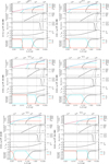 |
Fig. 3. Evolution of the modelled gas parameters, Z, nH, and NH, as a function of depth (AV) for a solar-metallicity cloud (top left) and for a cloud of 0.1 Z⊙ (top right), with a starting density of 103 cm−3 and rin of 1020.7 cm, G0 = 380 in terms of the Habing field. Two central panels: effect of density variations (left: nH = 102 cm−3; right: nH = 104 cm−3) for Z = 0.5 Z⊙ with G0 = 380. Bottom two panels: effect of G0 variations (left: G0 = 80; right: G0 = 1800) for constant Z (0.5 Z⊙) and constant nH (103 cm−3). Each panel contains subpanels within, from top to bottom: cumulative mass in the ionised, neutral atomic, and molecular phases; normalised cumulative intensity of the [C II]λ158 μm, [C I]λ610 μm, and CO (1−0) lines; abundance of C+, C0, and CO relative to C; hydrogen density (nH) as a function of column density (NH) and AV; fraction of hydrogen in the ionised, atomic, and molecular form. The vertical dashed lines indicate the depth of the main phase transitions: H+ to H0, H0 to H2, CO(1−0) optical depth of 1. Masses indicated here should be adjusted for individual galaxies, scaling as LTIR (galaxy)/109 L⊙, as the source luminosity of the model is 109 L⊙ (see Appendix A). |
To understand the effect of Z, nH, and G0 on the zone boundaries and accumulated mass, we compare three different cases in Fig. 3:
-
Metallicity effects: Compare Z = 1.0 Z⊙ (top left panel) and Z = 0.1 Z⊙ (top right panel) for a fixed nH (103 cm−3) and fixed G0 (380).
-
Density effects: Compare nH = 102 and 104 cm−3 with a fixed Z (0.5 Z⊙) and fixed G0 (380) (middle left and right panels).
-
G0 effects: Compare G0 varying from 80 to 1800 with a fixed Z (0.5 Z⊙) and fixed nH (103 cm−3) (bottom left and right panels). Here we provide an example that can be used to interpret these plots: in the case of Z = 1.0 Z⊙ (top left panel), the transition from H+ to H0 occurs at AV ∼ 0.015 mag and the transition from H0 to H2 is at AV ∼ 0.5 mag, while the C+-emitting zone spans the range of AV ∼ 0.05 to 2 mag. The evolution of the accumulated mass of the hydrogen species (top left panel, top subpanel) indicates that the C+-emitting zone includes ∼90% of the total gas mass in the form of both H0 and H2, while CO is not yet formed at those AV values. The C0-emitting region begins at AV ∼ 2 mag until CO forms (in a region containing exclusively H2). If we then lower the metallicity to 0.1 Z⊙ (top right panel), we see that the evolution of the C+-emitting zone and the H0 and H2 transitions in terms of AV are the same as the 1.0 Z⊙ case; however, the NH, or cloud depth, scales differently, requiring a larger cloud depth at 0.1 Z⊙ to reach the same AV as the 1.0 Z⊙ cloud.
The middle panels show how the cumulative [C II], [C I], and CO (1−0) intensities scale when changing only the nH in the ionised zone from 102 cm−3 (middle left panel) to 104 cm−3 (middle right panel), while keeping G0 and Z fixed. In this case, increasing the nH shifts the transitions from H+ to H0 and from H0 to H2 to lower values of AV. For the higher density case, we are quickly out of the H+ region and into the atomic regime. Also, as can be seen from the central right-hand panel, C+ is emitting over much of the H2 zone and before CO is emitted for the higher density case.
Finally, the bottom panels demonstrate the effect of changing G0 and keeping Z and nH fixed. The increase of G0 from 80 to 1800, for example, shifts the H+ to H0 transition to higher AV values (from AV ∼ 0.0015 to 0.02 mag) as well as a higher NH value for the H0 to H2 transition and with C+ tracing a lower mass of H2.
AV/NH is computed from the dust-to-gas ratio, which is assumed to be scaled by metallicity in the model for the range of metallicities studied here. For an H+ region, as long as dust does not significantly compete with hydrogen for ionising photons, the NH of the H+ region will remain constant. However, reducing the metallicity does reduce the AV corresponding to the NH in the H+ region by the same factor as the metallicity, and hence the ratio AV/NH. The size (in AV) of the C+ zone is roughly independent of metallicity (Kaufman et al. 2006), because the abundance of C+ scales directly with metallicity, while the UV opacity scales inversely. For Z = 0.1 Z⊙ the carbon abundance is reduced by a factor of ten, but the decrease in dust extinction means that C+ is formed over a path-length ten times longer than that for 1.0 Z⊙.
5.2. Hydrogen and carbon phase transitions in the model grids
Another way to visualise the model grids is shown in Fig. 4 with some observables, such as H I, [C II], [C I], LTIR, and [O I]λ63 μm. The y-axes of this figure show the L[C II]/LTIR (in percentage) versus H I and H2 gas mass reservoirs in the C+ and C0-emitting regions (defined above) extracted from Cloudy models for metallicities of Z = 0.05, 0.1, and 1.0 Z⊙ (from top to bottom) and for a range of G0 and nH. The last column shows the L[C II]/LTIR and L[C II]/L[O I] behaviour in terms of G0, nH, and Z. The total H2 gas mass from the model is shown in Col. 4 of Fig. 4 for the various metallicity bins. The C+-emitting region and some of the C0-emitting region, depending on Z, n, and G0 (Fig. 3), will harbour H2 sitting outside the CO-emitting region. We note that the models are scaled to LTIR of 109 L⊙. These diagrams can be used to bracket gas masses for a given L[C II]/LTIR and Z bin. To apply these models to observations of a specific galaxy, the masses must be scaled by the proper LTIR of the galaxy/109 L⊙. More Cloudy model details, including application of the scaling factor, are described in Appendix A. An example of the application of the model grids to the galaxy IIZw 40 is demonstrated in Fig. 7 and Sect. 6. A simple conversion of observed [C II], [C I], or CO (1−0) to mass of total H2 or fraction of CO-dark gas is not immediately straightforward.
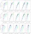 |
Fig. 4. Grids of Cloudy calculations: model L[C II]/LTIR vs. H I and H2 mass reservoirs in the C+, C0-emitting regions, total H2 mass, and L[C II]/L[O I] behaviour (last column) in terms of metallicities of Z = 0.05, 0.1, and 1.0 Z⊙ (from top to bottom) and for a range of G0 and nH, the initial hydrogen density. The colour coding in each figure is log nH/cm−3 which increases from 1.0 (green) to 4.0 (purple). A range of G0 is set by varying log rin/cm from 21.3 at the top right of the grids (large dots) to 20.0 at the bottom left of the grids (smaller dots). These rin values cover a range of log G0 of 1.25 to 4.06 (Sect. 5). The Cloudy models are run with a source luminosity of 109 L⊙. Thus, the output masses should be scaled likewise (see Appendix A for details). The models are run to log N(CO)/cm−2 = 17.8 (AV ∼ 10 mag) for these grids. |
5.2.1. Metallicity effects
As the metallicity decreases (from bottom to top panels in Fig. 4), the grids of gas mass shift to the right: more of the H2 is associated with the C+ and C0-emitting zones, demonstrating the overall larger CO-dark gas reservoirs predicted by the models in order to reach the molecular core. The location of both the H2 front and the formation of CO depend on metallicity, with both zones forming at higher AV with decreasing Z (Wolfire et al. 2010). The location of the H2 front as a function of AV depends only weakly on metallicity, scaling as ∼ln(Z−0.75). This is caused by the H2 formation rate scaling linearly with Z, while the UV dissociation rate of H2 depends on both the self-shielding of H2 (independent of Z) and dust extinction (which increases at a given depth with increasing Z). The CO-forming zone scales as ∼ln(Z−2) which is due to the decreased abundance of oxygen and carbon, which scale directly with Z. This has the overall effect of increasing the H2 zone. Additionally, our calculations compute density as a function of column density. Decreasing Z increases the column density needed to obtain the same AV (also in Fig. 3), therefore making the density in the H2 zone higher at lower metallicity. These combined effects increase the mass present in the H2 zone.
5.2.2. Distribution of the H0 and H2 phases
The first three columns of Fig. 4 show the consequence of metallicity on the partition of the mass between three regions, namely the H0 associated with [C II] emission, the H2 associated with [C II] emission, and the H2 associated with [C I] emission. The mass of H0 associated with [C II] increases significantly with decreasing metallicity, as expected. The beginning of the H0 zone starts at the hydrogen ionisation front, which for most of our parameter space is dominated by hydrogen opacity because the dust does not significantly compete with the gas for ionising photons. Therefore, the column density corresponding to the hydrogen ionisation front is nearly independent of Z, but the AV of the ionisation front will decrease with decreasing Z because of the lower AV/NH. The AV of the H2 front increases slightly with decreasing Z as a result of decreased dust extinction. Overall, these two processes lead to a larger H0 zone and, therefore, increased mass with decreasing Z. The size of the H2 zone, and the beginning of the CO-emitting region, follow similar logic.
5.2.3. G0 effects
When G0 increases (for the same density and Z), the H2 and CO fronts are pushed out to higher column densities, as expected because of the increased dissociation rate. The width (in AV) of the H2 zone therefore shows little variation with G0. Increasing G0 does have a mild effect on the mass associated with the H2 zone, with increasing G0 decreasing the mass in the H2 zone (Fig. 4). This is because increasing G0 moves the H2 zone out to a larger column density (Fig. 3). As the density in our models increases with increasing NH, the physical size of the H2 zone will shrink. The thinner physical size leads to a smaller integrated mass when compared to a lower G0 calculation. However, this effect is small when compared to variations of CO-dark mass with Z. Increasing density also slightly decreases the H2 region mass, which is due to slight changes in the location of the H2 front and the beginning of the CO formation zone.
5.2.4. Density effects
In addition to the size of each region, the temperature, nH, and G0 will dictate whether or not the H0, H2, and C+ regions will emit, and therefore, trace the CO-dark gas. For [C II], the emission is controlled by the C+ column density, the ncrit for [C II] emission (3 × 103 cm−3 for collisions with H0), and the excitation temperature (92 K) (Kaufman et al. 1999). We see that a density below the ncrit in the H0 region allows for efficient emission of [C II] (Fig. 3). This is reflected in the fact that, for the lower density models shown in Fig. 4, the H I mass and the H2 mass traced by [C II] are often comparable. For densities beyond ncrit, the emission of [C II] is nearly independent of nH, and is therefore controlled by the temperature and column density. Since the density increases with column density, for almost all models except the lowest density of 10 cm−3, the density in the H2 zone eventually exceeds ncrit of [C II], while for the H0 zone the column density is lower, leading to lower densities in this region and a larger region of the parameter space with a density lower than ncrit of [C II]. This explains why Fig. 4 has some spread in the mass for different densities, while for the H2, traced by [C II], the plot is nearly constant for decreasing Z, except for the lowest densities considered in our calculations. For Z = 1.0 Z⊙, slightly more spread is seen because the column density needed to reach the stopping criterion, and thus the density increase, is smaller. A similar effect occurs for the mass traced by [C I], which has a ncrit similar to [C II], thereby causing almost all of the lower metallicity calculations to be independent of nH. Overall, the reservoir of MH2 from which the C+ emission originates, is systematically lower than that of the C0-emitting zone. This effect is caused by the fact that where C0 is emitting, most of the hydrogen is in the form of H2 while in the C+-emitting region, a significant amount of the hydrogen is in the form of H I, not necessarily in H2, and the thickness of the respective layers are comparable.
The plots of the fifth column in Fig. 4 show the [C II]-to-[O I] ratio as a function of L[C II]/LTIR for the range of nH and G0. Kaufman et al. (1999) show that this ratio depends strongly on G0 for low density, especially for the higher Z case. Then, for increasing density the functional form of the ratio changes, becoming more sensitive to density for densities greater than the ncrit of [C II]. For larger densities, the [O I] emission increases with density, while the [C II] stays roughly constant (for a constant G0), leading to a lower [C II] to [O I] ratio. This explains the trend of this plot with decreasing Z, as the increased density in the PDR, given our density law, leads to models with an initially low density reaching the ncrit of [C II], which causes the predicted emission of [O I] to increase relative to [C II].
Figure 4 allows us to quantify the amount of gas mass accumulated until the stopping criterion of the model is reached (i.e. log N(CO) = 17.8; refer to Sect. 5.1) as a function of important physical parameters, given the observed FIR spectrum. For example, in the metallicity bin Z = 1.0 Z⊙, given an observed L[C II]/LTIR of 0.5%, the total mass of H2 gas ranges from 1 × 10⁸ to 3 × 10⁹ M⊙, depending on the density, while for the lowest metallicity bin shown, Z = 0.05 Z⊙, the quantity of H2 gas ranges from 1 to 3 × 10¹⁰ M⊙ for this same L[C II]/LTIR value. This shift to higher mass ranges of H2 gas suggests that the mass of CO-dark H2 gas can be an important component in low Z galaxies, as already pointed out in previous works (e.g. Papadopoulos et al. 2002; Wolfire et al. 2010).
In summary, from Fig. 4, the observed L[C II]/LTIR enables us to determine a range of plausible G0 and nH for a given metallicity. If G0 and nH can be determined from other assumptions or observations (e.g. [C II]/[O I] for density) then a tighter constraint for the total H2 gas can be determined (Sect. 5.4), eliminating some of the spread in nH and G0. For the lowest metallicity cases, the range of H2, determined by G0 and nH, is relatively narrow, and less dependent on variations in G0 or nH. Thus, even having only observations of [C II] and LTIR, Fig. 4 may bring a usefully narrow range of solutions for the total H2 for the lowest metallicity cases based on the definition of CO-dark gas adopted here and used by Wolfire et al. (2010).
5.3. How [C II], [C I], and CO (1−0) can trace MH2
We extract the [C II], CO (1−0), and [C I](1−0) (609 μm) luminosities at the model stopping depth of log N(CO) = 17.8 (AV ∼ 10 mag), inspecting the line luminosities as a function of MH2. In Fig. 5 we show the L[C II]/MH2, L[C I]/MH2, and LCO/MH2 conversion factors as a function of nH and G0 for the examples of Z = 1.0 Z⊙ and Z = 0.1 Z⊙. Caution must be exercised when using LCO/MH2 from these figures, because the MH2 within the CO-emitting region is very sensitive to the depth at which the models are stopped. If there is reason to trust that AV of ∼10 mag is an accurate representation of the CO-emitting zone, then the LCO/MH2 from this figure would be justifiable. It may not be applicable for some low Z cases, as discussed in Sect. 5.4.
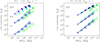 |
Fig. 5. Model grids that provide the L[C II], L[C I](1−0) (609 μm), and LCO – to – MH2 conversion factors for Z = 1.0 Z⊙ (left) and Z = 0.1 Z⊙ (right) for the particular model using a cloud depth of log N(CO)/cm−2 = 17.8. The colour coding refers to density values ranging from log nH/cm−3 = 1 (green) to 4 (purple). G0 increases with increasing symbol size, taking values of 5, 20, 100, 200, and 500. To obtain the total molecular gas mass, which would include He, an additional factor of 1.36 (Asplund et al. 2009) should also be included for the total mass. We note that MH2 in the CO-emitting region is very sensitive to the depth at which the models are stopped which corresponds to AV ∼ 10 mag here. |
We highlight the fact that the profiles shift to the right, to higher H2 masses at lower Z. For the higher Z case, density in particular plays an important role in determining the MH2 conversion factors for these species. For low Z, the density variations become less sensitive to the MH2, as noted in the Z = 0.1 Z⊙ case (right panel of Fig. 5). For the case of L[C I]/MH2 and LCO/MH2 at lower metallicity, the density contours collapse together (Fig. 5, right panel), as is the case for the L[C II], except for the highest nH case (nH = 104 cm−3; the green dots). In principle, [C I] should be able to quantify MH2, independent of density. From the right panel of Fig. 5, we derive a L[C I]/MH2 conversion factor for the case of Z = 0.1 Z⊙:
![$$ \begin{aligned} {M}_{\rm H_{2}} = 10^{4.06} \times {{L}_{\rm [C\,i\mathrm ]}}^{1.04}, \end{aligned} $$](/articles/aa/full_html/2020/11/aa38860-20/aa38860-20-eq1.gif)
where L[C I] is in units of L⊙ and MH2 is in units of M⊙. Considering the small effects of density and G0 on the L[C I]/MH2 conversion factor for this particular low-Z case, Eq. (1) determines MH2 from L[C I] with a standard deviation of 0.3 dex. The L[C II]/MH2 is about two orders of magnitude higher than L[C I]/MH2, while the LCO/MH2 is two orders of magnitude lower. [C I] appears to be a useful tracer to quantify the MH2, as also illustrated from hydrodynamical models (e.g. Glover & Clark 2016; Offner et al. 2014), and, as we show here at least for low-Z cases, with little dependence on nH. The fact that L[C I] is much fainter than L[C II] (Fig. 5) makes it more difficult to use as a reliable tracer of MH2. These effects can also be seen from the grids in Fig. 4.
We continue in the following sections to demonstrate the use of the observed [C II] to determine MH2 for specific cases and will follow up on [C I] as a tracer of MH2 in a subsequent publication.
5.4. How to determine AV and its effect on line emission (Spaghetti plots)
We see from Fig. 2 that L[C II]/LCO(1−0) exhibits great variation from galaxy to galaxy. When comparing the observed L[C II]/LCO(1−0) for low-metallicity galaxies (ranging from ∼3000 to 80 000), to the modelled L[C II]/LCO(1−0), where the stopping criterion is AV ∼ 10 mag, we see that the models do not reach such high observed L[C II]/LCO(1−0) values. This is because when the models are stopped at AV ∼10 mag, too much CO has already formed for the low-Z cases (Fig. 3), which require the models to stop at lower AV. The higher metallicity molecular clouds, exhibiting lower L[C II]/LCO(1−0) than the dwarf galaxies, could be better described by stopping at AV ∼ 10 mag. To explore the sensitivity of the emission as a function of depth, we can use the observed L[C II]/LCO(1−0) as a powerful constraint.
Figure 6 shows the model grid results for the L[C II]/LCO(1−0) and ratios of [C II], CO (1−0), [C I]λ609 μm, [O I]λ63 μm, and [O I]λ145 μm lines to MH2 as a function of AV for a range of nH (101, 102, 103, 104 cm−3) and G0 values (∼20, 500, 800) for Z = 0.05 Z⊙ (left column) and Z = 1.0 Z⊙ (right column). We can also understand the behaviour of these plots while referring to Fig. 3 and Sects. 5.1 and 5.2.
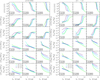 |
Fig. 6. “Spaghetti plots”: model results for L[C II]/LCO(1−0) and ratios of LCO/MH2, L[C I]λ609 μm/MH2, and L[O I]/MH2 as a function of AV for a range of nH (101, 102, 103, 104 cm−3) and G0 values (∼20, 500, 8000) for Z = 0.05 Z⊙ (left) and 1.0 Z⊙ (right). |
For example, when AV ∼ 1 mag is reached, [C II] formation is increasing rather linearly while CO increases exponentially (also evident in Fig. 3), and between AV ∼ 1 and 10 mag we see a rather linear decrease of L[C II]/LCO(1−0). The L[C II]/MH2 and L[O I]/MH2 continue to decrease beyond AV ∼ 1 mag because the [C II] and [O I] have stopped emitting but the MH2 continues to increase. The overall trend is therefore the drop in L[C II]/MH2 and L[O I]/MH2 for greater AV. Density can have a considerable effect on the [O I] emission, producing a wide spread of L[O I]/MH2 as AV increases for higher G0 environments. For example, for G0 of 8000 and AV ∼5, there is about 50 to 100 times greater L[O I]/MH2 for nH = 104 cm−3 compared to the case with nH = 101 cm−3 for Z = 0.5 and 1.0 Z⊙. Both [O I] lines behave similarly, with [O I]λ145 μm being generally weaker than [O I]λ63 μm by approximately one order of magnitude.
The L[C II]/LCO(1−0) is a good tracer of AV for all G0 and nH, with the range of AV becoming narrower for the spread of nH as G0 increases, as seen in the top panels of Fig. 6. The L[C I]/MH2 begins to turn over, peaking at AV of about a few magnitudes, approximately where the [C II] formation has decreased. This is why we see a relative flattening of the L[C I]/MH2 for growing AV.
We stop the plots in the figures beyond where CO has formed and becomes optically thick. Otherwise this MH2 will continue to accumulate causing the LCO/MH2 to turn over and begin to decrease beyond the point of τCO = 1. Having CO (1−0) observations in addition to the [C II] observations brings the best constraint on the AV of the cloud and thus a better quantification of the MH2.
We note that to construct Fig. 6, the models are stopped at log N(CO) = 17.8 (a maximum AV ∼ 10 mag) and the line intensities are extracted at the different depths into the cloud, that is, at different cloud AV values. In principle, the emerging line intensities could be different depending on the stopping criterion, due to optical depth effects and cloud temperature structure. To quantified this effect, we ran grids stopping at several maximum AV values (e.g. 2, 5, and 10 mag) and extracted line intensities, comparing the values we present in Fig. 65. The effects on the [O I] and [C II] line intensities are mostly negligible (variations < 20% throughout the grid). The intensities of the grid stopping at a maximum of AV of 2 mag are generally similar to or larger than the line intensities extracted at the cloud depth of AV = 2 mag of a grid stopping at maximum AV of 10 mag, primarily due to optical depth effects on the grids run to AV of 10 mag versus AV of 2 mag. The CO (1−0) can see up to a factor of 2.5 variations (primarily at AV = 2 mag) depending on the stopping criteria and the extraction of line intensities in AV construction. Our comparison verification has assured us that we can move forward with our use of Fig. 6.
Later, when the models are applied to particular observations (Sect. 6), the depth of the models, that is, the maximum AV, will be adapted for the specific metallicity case to determine the range of associated masses in the different zones. More precise determination of the stopping criterion will also require some knowledge of the range of G0 and nH (e.g. L[C II]/L[O I] in Fig. 4). Only then can we have the necessary ingredients to obtain the total MH2. Thus, determination of AV then gives us the total MH2. The mass of CO-dark H2 is then the difference between the total MH2 from the models and the H2 determined from the observed CO (1−0) using a Galactic XCO.
5.5. Quantification of the total MH2 and CO-dark gas: how to use the models
We walk through the steps to constrain the total MH2 and the CO-dark gas, depending on the availability of observations. We emphasise that to obtain the total molecular gas, including He, an additional factor of 1.36 (Asplund et al. 2009) should be taken into account. The best-constrained case is that for which [C II], [O I], CO (1−0), and LFIR observations exist. We also illustrate the range of solutions that can be obtained with less observational constraints.
Since metallicity plays an important role in the models, knowledge or assumptions of Z are necessary. The parameters that define the applicable model are G0, nH, and the maximum AV. We outline the steps to use the models:
– First we use the L[C II]/LFIR to find the range of G0 using Fig. 4. As can been seen in those figures the L[C II]/LFIR is most strongly dependent on the radiation field density and less so on density for a given Z.
– The second step is to further refine the corresponding model parameters with the L[C II]/L[O I] ratio (right-most panels in Fig. 4), or any combination of tracers that would provide the density in the [C II]-emitting zone of the PDR. For a given (range of) radiation field(s) this ratio is sensitive to the gas density. The combination of these two observational ratios generally constrains the radiation field and starting density well.
– Finally, the depth of the model (AV) can be found using the observed L[C II]/LCO(1−0) in combination with Fig. 6. The top series of panels shows the predicted line ratio for the different combinations of Z, G0, and nH.
These steps are illustrated for one galaxy, as an example, in Sect. 6 and Fig. 7.
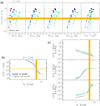 |
Fig. 7. Application of our model to the particular case of II Zw 40. Panels a show how the observed L[C II]/LTIR and L[C II]/L[O I] line ratios allow us to constrain nH and G0. Panel b shows how the L[C II]/LCO(1−0) ratio evolves in II Zw 40 as a function of AV, given the parameters previously derived from panel a. The green line indicates the best matching model. Panels c show the corresponding factors to convert L[C II], L[C I], and LCO to MH2 (see Sect. 6). |
Having found the parameter combination(s) that reproduce the relative strength of these key emission lines and the dust continuum, we can scale the model to the absolute line strength using the panels above and obtain the mass of H2. Probably the most useful scaling is based on using the L[C II]/MH2 predictions (fourth row of each panel in Fig. 6) because the [C II] line is strong and it originates throughout the parts of the model where the L[C II]/LCO(1−0) varies strongly. We note that our methodology using [C I] as an observational constraint does not (directly) aid in better determining the most applicable models in the range of interest, that is, those situations where the CO-emitting zone is reached. However, the conversion from [C I] line luminosity to molecular gas mass for the applicable models is tighter than for [C II] (see also Fig. 5). Therefore [C I] observations will be very useful for getting the best possible measures of the total H2 gas mass once the matching models have been determined and compared to observations. Once the total MH2 is determined, the difference between this value and the MH2 determined from CO (1−0) and the XCO conversion factor will quantify the CO-dark gas reservoir.
6. Applying the models: the particular example of II Zw 40
Here, we use one galaxy from the DGS, II Zw 40, (Z = 0.5 Z⊙), to demonstrate how to determine the total MH2 directly from the observations and the models presented above and thus the subsequent CO-dark gas mass. The relevant steps are visualised in Fig. 7, where the grids are run to a maximum depth of AV = 10 mag. We first obtain the fiducial model results for MH2 using the basic set of observational constraints: [C II], [O I], CO (1−0), and LFIR. It is often not possible to have all of these tracers. Therefore, we also explore the derived ranges of MH2 for II Zw 40 when limited observational data are available to constrain AV, nH, and G0. In this way we can get an idea of what kind of accuracy can be obtained with varying availability of constraints.
6.1. Fiducial model
The observed value of L[C II]/LTIR in II Zw 40 is 0.134 ± 0.024 (Cormier et al. 2015) which translates to a G0 of around 300 for the range of densities considered. The L[C II]/LTIR alone does not tightly constrain the density. In this case we also have the valuable [O I] line. The relatively high value of L[C II]/L[O I] (1.35 ± 0.29) matches the lower density models (log(nH) = 1.8, from interpolation; last panel of Fig. 7a).
We retain the models that match the combined L[C II]/LTIR and L[C II]/L[O I], that is, the models that cross the yellow intersection in the right-most panel of Fig. 7a. Figure 7b, extracted from Fig. 6, shows the behaviour of L[C II]/LCO(1−0) as a function of AV for these models in grey. The green line is the model curve of the best matching model. As can be seen, all models reproduce the observed L[C II]/LCO(1−0) (2.33 × 10⁵) at an AV value of ∼5 mag with a small dispersion.
Finally, the top panel of Fig. 7c shows that the L[C II]/MH2 for the best matching model depth is ∼0.01 [L⊙/M⊙] but values up to ∼0.02 are also compatible. The L[C II] of 3.87 × 10⁶ L⊙ of II Zw 40 translates to a total MH2 ranging from 1.3−5.1 × 10⁸ M⊙ with the best matching model yielding a MH2 of 3.2 × 10⁸ M⊙.
It is interesting to compare the derived H2 gas mass with that determined using LCO and a standard (Milky Way) XCO conversion factor6. The standard conversion factor yields a value of 7.1 × 10⁶ M⊙ which is only a few percent of the actual total H2 gas mass determined from these models. We already know that as Z decreases, XCO increases and calibrations for XCO based on metallicity vary wildly in the literature (e.g. Bolatto et al. 2013). Thus, comparing with a Galactic XCO really gives a lower limit on what is expected. In any case, even for the moderately low Z of 0.5 Z⊙, the CO-dark molecular gas will be important.
6.2. Estimating MH2 with fewer observational constraints
Following the full example for II Zw 40 above, we consider: case (a) when using [C II], CO (1−0), and LTIR (no [O I] line observed or no other density indicator) and case (b) where only [C II] and LTIR are available (CO (1−0) and [O I] are not available). In each case, we compare to the MH2 derived from our fiducial model above (Sect. 6.1), where a more complete set of observations ([C II], LTIR, [O I], and CO (1−0)) was available.
– case (a): Using [C II], LTIR, and CO (1−0). The observed ratio of L[C II]/LTIR for this galaxy (Fig. 7) indicates combinations of log(nH) and log(G0), from (1;2.2) through (2.5;2.8) to (4.0;3.3). For these models, AV values between 3.5 and 6 mag reproduce L[C II]/LCO(1−0) within its uncertainty. The best model, i.e. the closest predictions to the observed values, has an AV of 4.5 mag and contains 1.3 × 10⁸ M⊙ of H2. The H2 gas mass in the models that satisfactorily reproduces the observations ranges from 0.6 to 5.1 × 10⁸ M⊙. Comparing with the range we find for the fiducial model (1.3−5.1 × 10⁸ M⊙), we can see that the allowed range is significantly larger: the upper value is the same, but now allows a lower end of the range. In the particular case of II Zw 40 the higher density models that contain less MH2 gas before reaching the observed L[C II]/LCO(1−0) values cannot be excluded and the range is therefore expanded to lower values.
– case (b): Using [C II] and LTIR as the only available observational constraints; CO (1−0) has not been observed or with limited sensitivity and [O I] or another density tracer has not been observed. This means that we cannot exclude “normal” L[C II]/LCO(1−0) ratios and high optical depth. Without a constraint on the AV, these models can only be used to infer an upper limit on the MH2 in the PDR by integrating the model until τCO ≃ 1. The same combinations of nH and G0 as for case a yield upper limits on H2 gas masses of 0.7 to 13 × 108 M⊙. Removing the CO-bright H2 gas from these models by using the predicted LCO with a Galactic conversion factor yields upper limits on the dark H2 gas mass of 0.5 to 11 × 108 M⊙. Thus the derived upper limit of 13 × 108 M⊙ is significantly above the value we derive (3.2 ± 1.9 × 10⁸ M⊙) using the full set of constraints. Whether such an upper limit is useful will depend on the specific science question one is trying to address.
7. Quantification of the total MH2 and CO-dark gas in the Dwarf Galaxy Survey
To quantify the CO-dark gas of the DGS galaxies, we determine the predicted total MH2 for each DGS galaxy from the models (M(H2)total). We then compare this predicted total MH2 to the mass of the CO-bright H2, M(H2)CO, using the observed LCO and Galactic XCO. The mass of the CO-dark gas component, M(H2)dark, would then be the difference between the model-predicted M(H2)total reservoir and the observed M(H2)CO:

We note nH values in the range 100.5 − 103 cm−3 and G0 values of 102 − 103, which are determined from the Cormier et al. (2019) model solutions for the DGS galaxies, for metallicities ranging from near solar to ≈1/50 Z⊙7. We then extract the total MH2 for each galaxy from the corresponding model grids, applying the steps described above, to quantify the total MH2 consistent with the model solutions and consequently derive the CO-dark gas reservoir for each galaxy. Various galactic properties, observed and modelled parameters, and their relationships with the total H2 mass and CO-dark gas reservoirs are inspected (Figs. 8–10).
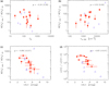 |
Fig. 8. Results from applying the models to the DGS sample and trends with model parameters. The vertical axis in panels a–c is M(H2)total/M(H2)CO (the ratio of the total MH2 determined from the model and the CO-bright MH2 determined from CO observations and the Galactic conversion factor) versus, on the horizontal axis, (a) G0, (b) density, and (c) AV. d: observed L[C II]/LCO(1−0) vs. model AV. Spearman correlation coefficients (ρ) and p-values in parenthesis are indicated within each panel. Red points are solutions for the DGS galaxies with CO detections. Open symbols are upper limits due to CO non-detections. The masses determined by the model for the individual galaxies have been scaled by their proper LTIR. |
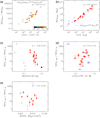 |
Fig. 9. Results for the DGS sample and trends with observable parameters. The vertical axis of panels a, c, d, and e is M(H2)total/M(H2)CO (total MH2 determined from the model over the MH2 determined from CO observations and the Galactic conversion factor). The horizontal axes of these same panels are as follows: a: L[C II]/LCO(1−0) with colour code for Z. The correlation shown in the dashed line is described in the panel in the equation for M(H2)total/M(H2)CO as a function of the observed L[C II]/LCO(1−0); standard deviation is 0.25 dex. b: total MH2 determined from the models vs. the observed L[C II]. Our resulting relationship of MH2 as a function of L[C II] is given within the panel; standard deviation is 0.14 dex. c: M(H2)total/M(H2)CO vs. Z; d: M(H2)total/M(H2)CO vs. observed L[C II]/LTIR. e: M(H2)total/M(H2)CO vs. ΣSFR, where SFR is determined from total IR luminosity from Rémy-Ruyer et al. (2015). Spearman correlation coefficients (ρ) and p-values in parenthesis are indicated within each panel. Red points are DGS galaxies with CO detections. Open symbols in all panels are upper limits due to CO non-detections. |
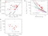 |
Fig. 10. Consequences of quantifying the total H2 of the DGS sample. a: Schmidt–Kennicutt relationship and Bigiel et al. (2008) revisited. Solid black squares are the values when the MH2 is calculated from the CO-to-H2 standard conversion factor; solid red dots are the total H2 determined from our self-consistent models. The dashed line is the usual Schmidt–Kennicutt relation, where low-Z star-forming dwarf galaxies are normally outliers when CO is used to determine the H2 (Cormier et al. 2014). The dotted line is the Bigiel et al. (2008) relationship determined for the ΣSFR − Σgas relationship. b: αCO as a function of Z from Schruba et al. (2012; black dotted line), Glover & Mac Low (2011; long black dashed line), Accurso et al. (2017a; blue dashed line), Amorín et al. (2016; green dashed line), Genzel et al. (2015; short black dashed line), Tacconi et al. (2018; orange dashed line), Bolatto et al. (2013; pink dashed line), and our new αCO − Z relationship determined from this paper (red dashed line). Red solid dots are the total H2 determined from our self-consistent models in this paper. Also given in the panel is the derived expression to determine αCO as a function of Z from this new relationship, which has a standard deviation of 0.32 dex. c: XCO conversion factor from this paper and ΣSFR. Spearman correlation coefficients (ρ) and p-values in parenthesis are indicated within each panel. Red dots are DGS galaxies with CO detections. Open symbols in all panels are upper limits due to CO non-detections. |
7.1. Trends of M(H2)total and CO-dark gas with model parameters
We notice right away (Fig. 8) that for DGS galaxies, M(H2)total is always much larger than that determined using CO only, M(H2)CO. The increasing M(H2)total/M(H2)CO signals the effect of the CO-dark gas reservoir becoming an increasingly important component of the total MH2, particularly in low-Z environments, which has been noted in the literature (e.g. Poglitsch et al. 1995; Israel et al. 1996; Madden et al. 1997; Wolfire et al. 2010; Fahrion et al. 2017; Nordon & Sternberg 2016; Accurso et al. 2017b; Jameson et al. 2018; Lebouteiller et al. 2019). The total mass of H2 can range from 5 to a few hundred times the H2 determined from the CO-emitting phase. The CO-dark gas dominates the total H2 reservoir in these galaxies. We are clearly missing the bulk of the H2 by observing only CO. What is controlling the fraction of CO-dark gas?
The G0 and density determined from the models do not seem to play an obvious role in driving the CO-dark gas fraction as shown in Fig. 8 panels a and b. Panel c shows the tight anti-correlation of M(H2)total/M(H2)CO with AV, and, as shown in panel d, AV anti-correlates with L[C II]/LCO(1−0), underscoring the role of AV in regulating the C+ – CO phase transition in the PDR (e.g. Wolfire et al. 2010; Nordon & Sternberg 2016; Jameson et al. 2018). The extreme range of observed L[C II]/LCO(1−0) in low-metallicity galaxies seen in Fig. 2 is a consequence of their overall low average effective AV.
7.2. Trends of M(H2)total and CO-dark gas with observables
What relationships exist between the observed quantities or measured galaxy properties and the total MH2 and the quantity of CO-dark gas? In Fig. 9 (panel a) we see that the observed L[C II]/LCO(1−0) is an excellent tracer of the CO-dark MH2 fraction. We fit this correlation to convert from observed L[C II]/LCO(1−0) to the M(H2)total/M(H2)CO:
![$$ \begin{aligned} M(\mathrm{H}_{2})_{\rm total}/M(\mathrm{H}_{2})_{\rm CO} = 10^{-3.14} \times [{L}_{\rm [C\,ii\mathrm ]}/{L}_{\rm CO(1{-}0)}]^{1.09}. \end{aligned} $$](/articles/aa/full_html/2020/11/aa38860-20/aa38860-20-eq3.gif)
The standard deviation of this fit is 0.25 dex. It follows from Eqs. (2) and (3) that the ratio of the mass of CO-dark gas to CO-bright gas is therefore:
![$$ \begin{aligned} M(\mathrm{H}_{2})_{\rm dark}/M(\mathrm{H}_{2})_{\rm CO} = 10^{-3.14} \times [{L}_{\rm [C\,ii\mathrm ]}/{L}_{\rm CO(1{-}0)}]^{1.09} - 1.0. \end{aligned} $$](/articles/aa/full_html/2020/11/aa38860-20/aa38860-20-eq4.gif)
We find a very tight correlation between L[C II] and total H2 gas mass (Fig. 9, panel b). The observed L[C II] can thus convert directly to totalMH2:
![$$ \begin{aligned} {M(\mathrm{H}_2)}_{\rm total} = 10^{2.12} \times [{L}_{\rm [C\,ii\mathrm ]}]^{0.97}, \end{aligned} $$](/articles/aa/full_html/2020/11/aa38860-20/aa38860-20-eq5.gif)
with a standard deviation of 0.14 dex. The C+ luminosity alone can pin down the total MH2, making the [C II]λ158 μm a valuable tracer to quantify the molecular gas mass in galaxies. Our modelling results find about a factor of three greater mass of total H2 associated with L[C II], and hence a larger reservoir of CO-dark gas mass, than that determined empirically from Zanella et al. (2018). These latter authors determine the MH2 from an assumed CO-to-MH2 conversion factor which is lower then that found in this study. We find a trend of the CO-dark MH2 fraction growing as the metallicity decreases (Fig. 9, panel c).
Our study of the lowest metallicity objects, however, is limited by the lack of robust CO detections in these extreme environments, thus limiting our knowledge of the behaviour of Z with the CO-dark gas mass or total MH2 at the lowest Z end. The CO-dark gas mass fraction does climb steeply as the Z decreases, even for moderately low-Z galaxies.
We see a weak trend of increasing fraction of CO-dark gas mass as the observed L[C II]/LTIR increases (Fig. 9, panel d). For the relatively narrow range of L[C II]/LTIR there is a wide range of CO-dark gas fraction. The fraction of CO-dark gas, which covers almost two orders of magnitude, does not show a trend with the approximately one order of magnitude range of surface density of SFR (ΣSFR) in our galaxy sample (Fig. 9, panel e). This is consistent with the effect of increasing L[C II]/LTIR (larger fraction of CO dark gas) being correlated with the increasing L[C II] (Fig. 9, panel d) and less so with direct effects of LTIR.
7.3. Consequences of the CO-dark gas fraction on the Schmidt–Kennicutt relation and the XCO conversion factor
What is the consequence of the presence of this reservoir of CO-dark H2 on ΣSFR and the surface density of gas (Σgas) in galaxies, as described in the relationships of Kennicutt (1998) and Bigiel et al. (2008)? In panel a of Fig. 10, we determine the ΣMH2 within the CO-emitting region (black squares) and find their positions to be well off of the ΣMH2 − ΣSFR relationships, as found by Cormier et al. (2014), which may be suggestive of much higher ΣSFR for their MH2. Once we take into account the total MH2 determined from [C II] and the modelling, which now includes the CO-dark MH2 as well as the CO-bright MH2 (Fig. 10, panel a; red dots), we see the locations of the galaxies shift to the right, lying between both ΣMH2 − ΣSFR relationships. The CO-dark gas is an important component to take into account in understanding the star formation activity in dwarf galaxies. While the data are limited, we find that taking into account the totalMH2, the star-forming dwarf galaxies do show a similar relation to that shown by the star-forming disc galaxies. Therefore, they are not necessarily more efficient in forming stars.
It has been shown from simulations (e.g. Glover & Clark 2012a; Krumholz et al. 2011) that star formation can proceed without a CO prerequisite, as well as without H2. The relationship observed between H2 and star formation can be due to the cloud conditions providing the ability to shield themselves from the UV radiation field, thereby allowing them to cool and form stars. In this process of shielding, at least H2 formation can also proceed, as well as CO in well-shielded environments. The conditions required to reach the necessary low gas temperatures set the stage for efficient C+ cooling. CO may accompany star formation but does not have a causality effect. Thus it may not come as a surprise to see star-forming dwarf galaxies that harbour a dearth of CO showing a similar relationship as that of the more metal-rich disc galaxies seen in the Schmidt–Kennicutt relationship.
With our determination of total H2 we can now give an analytic expression to convert from observed CO to a total MH2 conversion factor, αCO, and its relationship with Z. Here, again, the total MH2 now includes the CO-dark gas plus the CO-bright H2 mass. We find from Fig. 10 (panel b):
![$$ \begin{aligned} \alpha _{\rm CO} = 10^{0.58} \times [Z/Z_\odot ]^{-3.39}, \end{aligned} $$](/articles/aa/full_html/2020/11/aa38860-20/aa38860-20-eq6.gif)
with a standard deviation of 0.32 dex. We find a steeply rising αCO as the metallicity decreases. For example, at Z = 0.2 Z⊙, αCO is about two orders of magnitude greater than that for the Galaxy. A strong dependence of the CO-to-H2 conversion factor on metallicity is not unexpected. As the survival of molecules depends on how unsuccessful UV photons are in penetrating molecular clouds and photodissociating the molecules, extinction plays an important role in this process. Therefore, the lower dust abundance comes into play in the low-metallicity cases. In panel b of Fig. 10 we show a comparison of our derived metallicity dependence of αCO with others in the literature. Schruba et al. (2012) determined αCO from the observed SFR scaled by the observed LCO and a constant depletion time. This approach assumes that the efficiency of conversion of H2 into stars is constant within different environments. Our determination of αCO is relatively comparable to that of Schruba et al. (2012)8 given the spread of the observations, low number statistics, as well as possible uncertainties in metallicity calibrations. The αCO from our study seems to climb even more steeply toward lower Z. However, the lower end of the metallicity space, where mostly only upper limits in CO (1−0) observations exist, is not pinned down robustly. It is well shifted up from the Glover & Mac Low (2011) relationship with CO-to-MH2 conversion factor, which is determined from hydrodynamical simulations. A shallower slope is found for star-forming low-metallicity galaxies from Amorín et al. (2016) who derive a metallicity-dependent αCO considering the empirical correlations of SFR, CO depletion timescale, and metallicity. Other αCO − Z scaling functions, such as those of Arimoto et al. (1996) and Wolfire et al. (2010), fall near that of Amorín et al. (2016).
By studying how the molecular gas depletion times vary with redshift and their relation to the star-forming main sequence, Genzel et al. (2015) determined a scaling of αCO taking into account CO and dust-based observations (Fig. 10, panel b). While this conversion factor is shallower than the one we find from our study of local low-Z dwarf galaxies, these latter authors note that their study, which is based on massive star-forming galaxies, is probably not reliable for Z < 0.5 Z⊙. Accurso et al. (2017b) determine a comparable scaling of αCO with Z to that of Genzel et al. (2015) using similar surveys, but include a second-order dependence on distance from the star-forming main sequence in their αCO. Accurso et al. (2017b) caution against using this relation below Z ∼ 0.1 Z⊙, where it has not been calibrated. Bolatto et al. (2013) take a thorough look at numerous observations and theory and different metallicity regimes and propose a Z-dependent αCO which is similar to that of Genzel et al. (2015) for near-solar Z galaxies, but curves to steeper αCO for lower Z cases, while Tacconi et al. (2018) propose a compromise between those of Bolatto et al. (2013) and Genzel et al. (2015); see Fig. 10, panel b.
As soon as the ISM of the galaxy is more metal-poor, given the observed CO, which even for moderately metal-poor galaxies is difficult to obtain, the conversion factor from CO-to-H2 quickly grows. Even at 20% Z⊙, the CO conversion factor is already 1000 times that of our Galaxy. The true reservoir of MH2 may have been severely underestimated so far at low Z and these new relations can quantify that.
8. Possible caveats and limitations
While [C II] emission can be a convenient tool to quantify a reservoir of molecular gas that is not traced by CO (1−0), there are some caveats and limitations to this study.
– Lower metallicity bound: We emphasise that the relationships used to determine total gas mass presented here have only been studied for the star-forming dwarf galaxies of the DGS with metallicities as low as ≈1/50 Z⊙. The models have been applied for the low-metallicity galaxies for which CO is observed and this has limited the derived αCO and L[C II]-to-MH2 conversion factor only to metallicities as low as Z ∼ 0.2 Z⊙, even though [C II] has been detected in DGS galaxies below this metallicity.
– Limited range of model parameters: The models have been applied over a range of nH = 10 to 104 cm−3 and over a range of inner radii corresponding to log G0 ∼ 1 to 4. These results need to be studied over broader ranges of galactic properties to be applied with confidence beyond this study. For example, faint, low-metallicity, more quiescent dwarf galaxies can also harbour star formation rates lower than those found for the Schmidt–Kennicutt relation (e.g. Roychowdhury et al. 2009; Cigan et al. 2016), in contrast to the DGS sample (Fig. 10, panel a). Some of these more quiescent dwarf galaxies are at the lowest metallicity range explored here and do not have CO detections, but may also be harbouring some CO-dark molecular gas. Likewise, more massive, CO-rich galaxies have yet to be tested with this model.
– Galactic size scales: These conclusions have been drawn on unresolved galaxy scales. The reliability of [C II] to trace MH2 on resolved scales using these models has not been tested. A similar approach was carried out at 10 pc resolution in the 30Doradus region of the low-metallicity LMC (Z = 0.5 Z⊙), where > 75% of the H2 was CO-dark and traced by [C II] (Chevance et al. 2020). Considering that the [C II] emission is expected to be more extended than the CO (1−0) (e.g. Jameson et al. 2018; Chevance et al. 2020), our simple scheme using Cloudy and representing galaxies with a single H II region + molecular cloud in one dimension does not account for realistic geometry and for the physical mixing of different physical components and thus mixing G0 and nH conditions.
– The origin of [C II] emission in galaxies: We note that [C II] can arise from other components in galaxies, not only from neutral PDRs. For example [C II] can originate in the low-density ionised gas component in galaxies that is excited by electrons. In principle, to use [C II] to quantify the MH2, it is necessary to first determine whether or not there is “contamination” of the [C II] emission arising from the ionised gas which should first be removed before application of the model. This requires observations of other ionised gas tracers, such as the commonly used FIR [N II] lines, for example. Such studies often conclude that most of the [C II] emission in galaxies arises from PDR regions, with a decreasing fraction of the total [C II] emission arising from the ionised gas with decreasing metallicity (Kaufman et al. 2006; Croxall et al. 2017; Jameson et al. 2018; Cormier et al. 2019; Herrera-Camus et al. 2016; Accurso et al. 2017a; Sutter et al. 2019). Also, in our study we have not taken into account any contributing molecular gas reservoirs originating in the WNM or CNM atomic phases. The atomic gas component in our Galaxy has been proposed to harbour almost 50% of dark molecular gas of MH2 (e.g. Kalberla et al. 2020). We do extract the H I mass from the models, but with the observations of our global studies we cannot yet explore this component. Most of the H I in the dwarf galaxies arises throughout the galaxies and often from a very extended component – extending well beyond the [C II] emission. We do not resolve the H I associated with the PDRs and therefore cannot address this point.
– Metallicity calibrations: A word of caution related to metallicity determination is necessary when applying these scaling relations. Metallicity calibrations are well known to differ (e.g. Kewley & Ellison 2008) and where absolute calibrations differ significantly, this should be taken into account when looking into detailed application of the models.
While this study points to the usefulness of [C II] as a tracer of the molecular gas in low-Z galaxies, enlarging the galactic parameter space will be needed to apply these findings in a more general sense to a wide variety of galaxies, especially galaxies more massive than the dwarf galaxies in this study. Here, we only focus on galaxies of the local universe. However, this is already a potential step forward in the possibility of estimating the gas mass from high-z galaxies using ALMA to access the [C II]λ158 μm in the cases where CO (1−0) may be faint, perhaps due to lower metallicity.
9. Summary and conclusions
This study is motivated by the extreme L[C II]/LCO(1−0) values observed for low-metallicity galaxies, almost reaching 105 on global scales, which can be up to an order of magnitude higher than dustier star-forming galaxies. The bright [C II]λ158 μm lines observed in low-metallicity galaxies have been challenging to reconcile with the faint or undetectable CO (1−0) in light of their star formation activity. We have investigated the effects of metallicity, gas density, and radiation field on the total molecular gas reservoir in galaxies and quantified the mass of H2 not traced by CO (1−0), that is, the CO-dark molecular gas that can be traced by [C II]. We inspected Cloudy grids traversing these physical parameters in order to understand the behaviour of observed quantities, such as [O I], [C I], CO (1−0), [C II], and LFIR in terms of MH2 as a function of AV, metallicity and nH. In principle, [C I] can be an important tracer of the CO-dark molecular gas, and this will be further investigated in a follow-up study. However, due to its higher luminosity, [C II] is an ideal tracer of the molecular gas. We give recipes on how to use these models to go from observations to total MH2. We apply the models to the Herschel DGS, extracting the total MH2 for each galaxy. The CO-dark MH2 is then determined from the difference between the total MH2 and the CO-bright H2 traced by the observed CO (1−0). Our findings indicate that CO (1−0) in the dwarf galaxies traces only a small fraction of the H2, if any, while the total MH2 is dominated by the CO-dark gas which can be uncovered by [C II] observations.
We have determined a L[C II]-to-MH2 conversion factor: M(H2)total = 102.12 × [L[C II]]0.97 with a standard deviation of 0.14 dex. Following from this, we give a new CO-to-MH2 conversion factor that takes into account the total MH2 –both the CO-dark and CO-bright gas– given by application of the models:
αCO = 100.58 × [Z/Z⊙]−3.39 with a standard deviation of 0.32 dex.
Comparisons with the fraction of CO-dark gas in the low-metallicity galaxies and their galactic properties reveal the following findings:
1. The fraction of CO-dark gas is correlated with L[C II]/LCO(1−0). There is a tight correlation between the [C II]λ158 μm and the total MH2 over the range of low-metallicity galaxies of the DGS.
2. The effective AV from our models is anticorrelated with L[C II]/LCO(1−0) and hence the CO-dark gas fraction. Therefore, the consequence of the effective low AV overall in low-metallicity galaxies is the extreme L[C II]/LCO(1−0) observed in star-forming dwarf galaxies.
3. The SFR, nH, and G0 do not individually control the CO-dark gas mass fraction.
4. The CO-dark gas accounts for most (> 70%) of the total H2 over the wide range of galaxy properties of the Herschel DGS. This study consists of galaxies with L[C II]/LTIR ranging between 0.1 and 0.5%, metallicity values from ∼0.02 to 0.6 Z⊙, L[C II]/LCO(1−0) values corresponding to two orders of magnitude of MH2 and over three orders of magnitude of LFIR and stellar mass.
5. Our new CO (1−0)-to-MH2 conversion factor as a function of metallicity, which also accounts for the CO-dark MH2, is steeper than most others in the literature, but resembles that of Schruba et al. (2012).
6. When taking into account this significant CO-dark H2 reservoir, the star-forming dwarf galaxies, which were above the Schmidt–Kennicutt relation when only the observed CO (1−0) was used to deduce the H2 reservoir, now shift to the normal relation of ΣSFR − ΣMH2 found for star-forming disc galaxies.
7. [C I] shows signs of being a convenient tracer of the MH2, particularly at low Z where it can be independent of nH and G0. However, [C I] is intrinsically less luminous than [C II]. The utility of [C I] as a tracer of total MH2 for a variety of galactic conditions requires further follow-up investigation.
We conclude that the low LCO/SFR and the high L[C II]/LCO(1−0) observed in low-metallicity dwarf galaxies can be explained by the photodissociation of CO, and signals the presence of a prominent reservoir of CO-dark H2. Observations of a larger number of extremely low-Z galaxies is necessary to pin down the lowest Z end of the αCO − Z and the ![$ L_\mathrm{[C\,\textsc{ii}]}{-}M_\mathrm{H_{2}} $](/articles/aa/full_html/2020/11/aa38860-20/aa38860-20-eq7.gif) relations as well as to expand the studies of parameter space and spatial scales in galaxies. Likewise, robust comparison of other methods to determine MH2, and determination of when these different methods are applicable, will be the subject of followup studies.
relations as well as to expand the studies of parameter space and spatial scales in galaxies. Likewise, robust comparison of other methods to determine MH2, and determination of when these different methods are applicable, will be the subject of followup studies.
1 G0 = 1.6 × 10⁻³ erg cm−2 s−1, integrated over the energy range 6−13.6 eV (Habing 1968).
We note that for historical reasons, we use LFIR when comparing observations of the DGS to other observations collected in the literature over the years, originally presented with LFIR, such as Fig. 2, adapting LFIR and LTIR as per Rémy-Ruyer et al. (2013, 2015). However, this study uses LTIR (3 to 1100 μm), which is more commonly used today.
We assume solar O/H = 4.9 × 10⁻⁴ (Asplund et al. 2009); i.e. 12 + log(O/H)⊙ = 8.69.
To apply to specific cases where AV is not necessarily ∼10 mag requires running the model to different cloud depths, as we discuss in Sect. 5.4, where we quantify the MH2 of the individual DGS galaxies.
In this study, for the standard XCO conversion we use a factor of 2 × 1020 cm−2(K km s−1)−1 in terms of XCO (ICO ∝ NH2); 3.2 M⊙ pc−2(K km s−1)−1 in terms of αCO (ICO ∝ MH2). While αCO is normally 4.3 M⊙ pc−2(K km s−1)−1, including helium, here we do not include the helium mass (factor of 1.36) when comparing to the model output of MH2.
Metallicity values for the DGS galaxies are from Madden et al. (2013) which uses the strong line metallcity calibration from Pilyugin & Thuan (2005).
While different relations have been shown for different categories of galaxies in Schruba et al. (2012), here we use the relation given for all of the galaxies in that study.
Acknowledgments
The authors wish to thank the anonymous referee for a number of suggestions that have improved the presentation of this study. We thank A. Poglitsch for valuable discussions that also helped to improve the quality of the paper. We acknowledge support from the DAAD/PROCOPE projects 57210883/35265PE and from the Programme National Physique et Chimie du Milieu Interstellaire (PCMI) of CNRS/INSU with INC/INP co-funded by CEA and CNES. The European Unions Horizon 2020 research and innovation program under the Marie Sklodowska-Curie grant agreement No 702622 supported DC during this study. SH acknowledges financial support from DFG programme HO 5475/2-1. MC acknowledges funding from the Deutsche Forschungsgemeinschaft (DFG, German Research Foundation) through an Emmy Noether Research Group (grant number KR4801/1-1) and the DFG Sachbeihilfe (grant number KR4801/2-1). MG has received funding from the European Research Council (ERC) under the 397 European Union Horizon 2020 research and innovation programme (MagneticYSOs project, grant agreement 398 No 679937). FLP acknowledges funding from the ANR grant LYRICS (ANR-16-CE31- 0011). This research was originally made possible through the financial support of the Agence Nationale de la Recherche (ANR) through the programme SYMPATICO (Program Blanc Projet NR-11-BS56-0023) and through the EU FP7. This study made use of Herschel observations: PACS was developed by MPE (Germany); UVIE (Austria); KU Leuven, CSL, IMEC (Belgium); CEA, LAM (France); MPIA (Germany); INAFIFSI/OAA/OAP/OAT, LENS, SISSA (Italy); IAC (Spain). This development was supported by BMVIT (Austria), ESA-PRODEX (Belgium), CEA/CNES (France), DLR (Germany), ASI/INAF (Italy), and CICYT/MCYT (Spain). SPIRE was developed by Cardiff University (UK); Univ. Lethbridge (Canada); NAOC (China); CEA, LAM (France); IFSI, Univ. Padua (Italy); IAC (Spain); SNSB (Sweden); Imperial College London, RAL, UCL-MSSL, UKATC, Univ. Sussex (UK) and Caltech, JPL, NHSC, Univ. Colorado (USA). This development was supported by CSA (Canada); NAOC (China); CEA, CNES, CNRS (France); ASI (Italy); MCINN (Spain); Stockholm Observatory (Sweden); STFC (UK); and NASA (USA).
References
- Accurso, G., Saintonge, A., Catinella, B., et al. 2017a, MNRAS, 470, 4750 [NASA ADS] [Google Scholar]
- Accurso, G., Saintonge, A., Bisbas, T. G., & Viti, S. 2017b, MNRAS, 464, 3315 [NASA ADS] [CrossRef] [Google Scholar]
- Ackermann, M., Ajello, M., Allafort, A., et al. 2012, A&A, 538, A71 [NASA ADS] [CrossRef] [EDP Sciences] [Google Scholar]
- Allen, R. J., Hogg, D. E., & Engelke, P. D. 2015, AJ, 149, 123 [NASA ADS] [CrossRef] [Google Scholar]
- Amorín, R., Muñoz-Tuñón, C., Aguerri, J. A. L., & Planesas, P. 2016, A&A, 588, A23 [NASA ADS] [CrossRef] [EDP Sciences] [Google Scholar]
- Andreani, P., Retana-Montenegro, E., Zhang, Z.-Y., et al. 2018, A&A, 615, A142 [NASA ADS] [CrossRef] [EDP Sciences] [Google Scholar]
- Arimoto, N., Sofue, Y., & Tsujimoto, T. 1996, PASJ, 48, 275 [NASA ADS] [CrossRef] [Google Scholar]
- Asplund, M., Grevesse, N., Sauval, A. J., & Scott, P. 2009, ARA&A, 47, 481 [NASA ADS] [CrossRef] [Google Scholar]
- Bertemes, C., Wuyts, S., Lutz, D., et al. 2018, MNRAS, 478, 1442 [NASA ADS] [CrossRef] [Google Scholar]
- Bethermin, M., Fudamoto, Y., Ginolfi, M., et al. 2020, A&A, 643, A2 [CrossRef] [EDP Sciences] [Google Scholar]
- Bigiel, F., Leroy, A., Walter, F., et al. 2008, AJ, 136, 2846 [NASA ADS] [CrossRef] [Google Scholar]
- Bigiel, F., Leroy, A. K., Walter, F., et al. 2011, ApJ, 730, L13 [NASA ADS] [CrossRef] [Google Scholar]
- Bisbas, T. G., van Dishoeck, E. F., Papadopoulos, P. P., et al. 2017, ApJ, 839, 90 [NASA ADS] [CrossRef] [Google Scholar]
- Bolatto, A. D., Wolfire, M., & Leroy, A. K. 2013, ARA&A, 51, 207 [Google Scholar]
- Bothwell, M. S., Aguirre, J. E., Aravena, M., et al. 2017, MNRAS, 466, 2825 [Google Scholar]
- Bourne, N., Dunne, L., Bendo, G. J., et al. 2013, MNRAS, 436, 479 [NASA ADS] [CrossRef] [Google Scholar]
- Bourne, N., Dunlop, J. S., Simpson, J. M., et al. 2019, MNRAS, 482, 3135 [Google Scholar]
- Brauher, J. R., Dale, D. A., & Helou, G. 2008, ApJS, 178, 280 [NASA ADS] [CrossRef] [Google Scholar]
- Carilli, C. L., & Walter, F. 2013, ARA&A, 51, 105 [NASA ADS] [CrossRef] [EDP Sciences] [Google Scholar]
- Chevance, M., Madden, S. C., Lebouteiller, V., et al. 2016, A&A, 590, A36 [NASA ADS] [CrossRef] [EDP Sciences] [Google Scholar]
- Chevance, M., Madden, S. C., Fischer, C., et al. 2020, MNRAS, 494, 5279 [CrossRef] [Google Scholar]
- Cigan, P., Young, L., Cormier, D., et al. 2016, AJ, 151, 14 [NASA ADS] [CrossRef] [Google Scholar]
- Clark, P. C., & Glover, S. C. O. 2015, MNRAS, 452, 2057 [NASA ADS] [CrossRef] [Google Scholar]
- Combes, F., García-Burillo, S., Braine, J., et al. 2013, A&A, 550, A41 [NASA ADS] [CrossRef] [EDP Sciences] [Google Scholar]
- Cormier, D., Madden, S. C., Hony, S., et al. 2010, A&A, 518, L57 [NASA ADS] [CrossRef] [EDP Sciences] [Google Scholar]
- Cormier, D., Lebouteiller, V., Madden, S. C., et al. 2012, A&A, 548, A20 [NASA ADS] [CrossRef] [EDP Sciences] [Google Scholar]
- Cormier, D., Madden, S. C., Lebouteiller, V., et al. 2014, A&A, 564, A121 [NASA ADS] [CrossRef] [EDP Sciences] [Google Scholar]
- Cormier, D., Madden, S. C., Lebouteiller, V., et al. 2015, A&A, 578, A53 [NASA ADS] [CrossRef] [EDP Sciences] [Google Scholar]
- Cormier, D., Bigiel, F., Wang, J., et al. 2016, MNRAS, 463, 1724 [CrossRef] [Google Scholar]
- Cormier, D., Abel, N. P., Hony, S., et al. 2019, A&A, 626, A23 [NASA ADS] [CrossRef] [EDP Sciences] [Google Scholar]
- Croxall, K. V., Smith, J. D., Wolfire, M. G., et al. 2012, ApJ, 747, 81 [NASA ADS] [CrossRef] [Google Scholar]
- Croxall, K. V., Smith, J. D., Pellegrini, E., et al. 2017, ApJ, 845, 96 [NASA ADS] [CrossRef] [Google Scholar]
- da Cunha, E., Groves, B., Walter, F., et al. 2013, ApJ, 766, 13 [Google Scholar]
- Daddi, E., Bournaud, F., Walter, F., et al. 2010, ApJ, 713, 686 [NASA ADS] [CrossRef] [Google Scholar]
- Daddi, E., Dannerbauer, H., Liu, D., et al. 2015, A&A, 577, A46 [NASA ADS] [CrossRef] [EDP Sciences] [Google Scholar]
- Dale, D. A., Aniano, G., Engelbracht, C. W., et al. 2012, ApJ, 745, 95 [NASA ADS] [CrossRef] [Google Scholar]
- de Looze, I., Baes, M., Bendo, G. J., Cortese, L., & Fritz, J. 2011, MNRAS, 416, 2712 [Google Scholar]
- De Looze, I., Cormier, D., Lebouteiller, V., et al. 2014, A&A, 568, A62 [NASA ADS] [CrossRef] [EDP Sciences] [Google Scholar]
- Dessauges-Zavadsky, M., Ginolfi, M., Pozzi, F., et al. 2020, A&A, 643, A5 [CrossRef] [EDP Sciences] [Google Scholar]
- Díaz-Santos, T., Armus, L., Charmandaris, V., et al. 2017, ApJ, 846, 32 [Google Scholar]
- Eales, S., Smith, M. W. L., Auld, R., et al. 2012, ApJ, 761, 168 [NASA ADS] [CrossRef] [Google Scholar]
- Fahrion, K., Cormier, D., Bigiel, F., et al. 2017, A&A, 599, A9 [NASA ADS] [CrossRef] [EDP Sciences] [Google Scholar]
- Ferland, G. J., Chatzikos, M., Guzmán, F., et al. 2017, Rev. Mex. Astron. Astrofis., 53, 385 [NASA ADS] [Google Scholar]
- Franeck, A., Walch, S., Seifried, D., et al. 2018, MNRAS, 481, 4277 [NASA ADS] [CrossRef] [Google Scholar]
- Galametz, M., Madden, S. C., Galliano, F., et al. 2011, A&A, 532, A56 [NASA ADS] [CrossRef] [EDP Sciences] [Google Scholar]
- Gallerani, S., Ferrara, A., Neri, R., & Maiolino, R. 2014, MNRAS, 445, 2848 [Google Scholar]
- Galliano, F., Galametz, M., & Jones, A. P. 2018, ARA&A, 56, 673 [Google Scholar]
- Genzel, R., Tacconi, L. J., Combes, F., et al. 2012, ApJ, 746, 69 [Google Scholar]
- Genzel, R., Tacconi, L. J., Lutz, D., et al. 2015, ApJ, 800, 20 [Google Scholar]
- Glover, S. C. O., & Clark, P. C. 2012a, MNRAS, 426, 377 [Google Scholar]
- Glover, S. C. O., & Clark, P. C. 2012b, MNRAS, 421, 9 [NASA ADS] [Google Scholar]
- Glover, S. C. O., & Clark, P. C. 2016, MNRAS, 456, 3596 [Google Scholar]
- Glover, S. C. O., & Mac Low, M.-M. 2011, MNRAS, 412, 337 [Google Scholar]
- Gnedin, N. Y., & Draine, B. T. 2014, ApJ, 795, 37 [Google Scholar]
- Gong, M., Ostriker, E. C., & Kim, C.-G. 2018, ApJ, 858, 16 [Google Scholar]
- Grenier, I. A., Casandjian, J.-M., & Terrier, R. 2005, Science, 307, 1292 [Google Scholar]
- Griffin, M. J., Abergel, A., Abreu, A., et al. 2010, A&A, 518, L3 [EDP Sciences] [Google Scholar]
- Grossi, M., Corbelli, E., Bizzocchi, L., et al. 2016, A&A, 590, A27 [NASA ADS] [CrossRef] [EDP Sciences] [Google Scholar]
- Groves, B. A., Schinnerer, E., Leroy, A., et al. 2015, ApJ, 799, 96 [Google Scholar]
- Gullberg, B., De Breuck, C., Vieira, J. D., et al. 2015, MNRAS, 449, 2883 [Google Scholar]
- Habing, H. J. 1968, Bull. Astron. Inst. Neth., 19, 421 [Google Scholar]
- Hailey-Dunsheath, S., Nikola, T., Stacey, G. J., et al. 2010, ApJ, 714, L162 [Google Scholar]
- Harikane, Y., Ouchi, M., Inoue, A. K., et al. 2020, ApJ, 896, 93 [Google Scholar]
- Hashimoto, T., Inoue, A. K., Mawatari, K., et al. 2019, PASJ, 71, 71 [Google Scholar]
- Hayashi, K., Mizuno, T., Fukui, Y., et al. 2019, ApJ, 884, 130 [Google Scholar]
- Heintz, K. E., & Watson, D. 2020, ApJ, 889, L7 [Google Scholar]
- Herrera-Camus, R., Bolatto, A. D., Wolfire, M. G., et al. 2015, ApJ, 800, 1 [Google Scholar]
- Herrera-Camus, R., Bolatto, A., Smith, J. D., et al. 2016, ApJ, 826, 175 [Google Scholar]
- Hunt, L. K., García-Burillo, S., Casasola, V., et al. 2015, A&A, 583, A114 [NASA ADS] [CrossRef] [EDP Sciences] [Google Scholar]
- Hunter, D. A., Kaufman, M., Hollenbach, D. J., et al. 2001, ApJ, 553, 121 [Google Scholar]
- Israel, F. P., Maloney, P. R., Geis, N., et al. 1996, ApJ, 465, 738 [Google Scholar]
- Jameson, K. E., Bolatto, A. D., Wolfire, M., et al. 2018, ApJ, 853, 111 [Google Scholar]
- Jiao, Q., Zhao, Y., Lu, N., et al. 2019, ApJ, 880, 133 [Google Scholar]
- Kalberla, P. M. W., Kerp, J., & Haud, U. 2020, A&A, 639, A26 [EDP Sciences] [Google Scholar]
- Kamenetzky, J., Rangwala, N., & Glenn, J. 2017, MNRAS, 471, 2917 [Google Scholar]
- Kamenetzky, J., Privon, G. C., & Narayanan, D. 2018, ApJ, 859, 9 [Google Scholar]
- Kaufman, M. J., Wolfire, M. G., Hollenbach, D. J., & Luhman, M. L. 1999, ApJ, 527, 795 [Google Scholar]
- Kaufman, M. J., Wolfire, M. G., & Hollenbach, D. J. 2006, ApJ, 644, 283 [Google Scholar]
- Kennicutt, R. C., Jr. 1998, ARA&A, 36, 189 [Google Scholar]
- Kennicutt, R. C., Jr., & Evans, N. J. 2012, ARA&A, 50, 531 [Google Scholar]
- Kennicutt, R. C., Jr., Calzetti, D., Walter, F., et al. 2007, ApJ, 671, 333 [Google Scholar]
- Kewley, L. J., & Ellison, S. L. 2008, ApJ, 681, 1183 [Google Scholar]
- Krumholz, M. R., & Gnedin, N. Y. 2011, ApJ, 729, 36 [Google Scholar]
- Krumholz, M. R., Leroy, A. K., & McKee, C. F. 2011, ApJ, 731, 25 [Google Scholar]
- Kumari, N., Irwin, M. J., & James, B. L. 2020, A&A, 634, A24 [EDP Sciences] [Google Scholar]
- Langer, W. D., Velusamy, T., Pineda, J. L., et al. 2010, A&A, 521, L17 [Google Scholar]
- Langer, W. D., Velusamy, T., Pineda, J. L., Willacy, K., & Goldsmith, P. F. 2014, A&A, 561, A122 [NASA ADS] [CrossRef] [EDP Sciences] [Google Scholar]
- Lapham, R. C., Young, L. M., & Crocker, A. 2017, ApJ, 840, 51 [Google Scholar]
- Laporte, N., Katz, H., Ellis, R. S., et al. 2019, MNRAS, 487, L81 [Google Scholar]
- Lebouteiller, V., Cormier, D., Madden, S. C., et al. 2012, A&A, 548, A91 [NASA ADS] [CrossRef] [EDP Sciences] [Google Scholar]
- Lebouteiller, V., Cormier, D., Madden, S. C., et al. 2019, A&A, 632, A106 [EDP Sciences] [Google Scholar]
- Leitherer, C., Ortiz Otálvaro, P. A., Bresolin, F., et al. 2010, ApJS, 189, 309 [Google Scholar]
- Leroy, A. K., Walter, F., Brinks, E., et al. 2008, AJ, 136, 2782 [Google Scholar]
- Leroy, A. K., Bolatto, A., Bot, C., et al. 2009, ApJ, 702, 352 [Google Scholar]
- Leroy, A. K., Bolatto, A., Gordon, K., et al. 2011, ApJ, 737, 12 [Google Scholar]
- Leroy, A. K., Bigiel, F., de Blok, W. J. G., et al. 2012, AJ, 144, 3 [Google Scholar]
- Leroy, A. K., Walter, F., Sandstrom, K., et al. 2013, AJ, 146, 19 [Google Scholar]
- Li, Q., Narayanan, D., Davè, R., & Krumholz, M. R. 2018, ApJ, 869, 73 [Google Scholar]
- Liang, L., Feldmann, R., Faucher-Giguère, C.-A., et al. 2018, MNRAS, 478, L83 [Google Scholar]
- Liszt, H., Gerin, M., & Grenier, I. 2019, A&A, 627, A95 [Google Scholar]
- Lucas, R., & Liszt, H. 1996, A&A, 307, 237 [NASA ADS] [Google Scholar]
- Luhman, M. L., Satyapal, S., Fischer, J., et al. 2003, ApJ, 594, 758 [Google Scholar]
- Madden, S. C. 2000, New Astron. Rev., 44, 249 [Google Scholar]
- Madden, S. C., & Cormier, D. 2019, in Dwarf Galaxies: From the Deep Universe to the Present, eds. K. B. W. McQuinn, & S. Stierwalt, IAU Symp., 344, 240 [Google Scholar]
- Madden, S. C., Poglitsch, A., Geis, N., Stacey, G. J., & Townes, C. H. 1997, ApJ, 483, 200 [NASA ADS] [CrossRef] [MathSciNet] [Google Scholar]
- Madden, S. C., Galametz, M., Cormier, D., et al. 2011, in EAS Publications Series, eds. M. Röllig, R. Simon, V. Ossenkopf, & J. Stutzki, 52, 95 [CrossRef] [EDP Sciences] [Google Scholar]
- Madden, S. C., Rémy-Ruyer, A., Galametz, M., et al. 2013, PASP, 125, 600 [NASA ADS] [CrossRef] [Google Scholar]
- Magdis, G. E., Daddi, E., Elbaz, D., et al. 2011, ApJ, 740, L15 [NASA ADS] [CrossRef] [Google Scholar]
- Magnelli, B., Saintonge, A., Lutz, D., et al. 2012, A&A, 548, A22 [NASA ADS] [CrossRef] [EDP Sciences] [Google Scholar]
- Malhotra, S., Kaufman, M. J., Hollenbach, D., et al. 2001, ApJ, 561, 766 [Google Scholar]
- Maloney, P., & Black, J. H. 1988, ApJ, 325, 389 [NASA ADS] [CrossRef] [Google Scholar]
- Murray, C. E., Peek, J. E. G., Lee, M.-Y., & Stanimirović, S. 2018, ApJ, 862, 131 [NASA ADS] [CrossRef] [Google Scholar]
- Narayanan, D., Bothwell, M., & Davé, R. 2012, MNRAS, 426, 1178 [NASA ADS] [CrossRef] [Google Scholar]
- Nesvadba, N. P. H., Cañameras, R., Kneissl, R., et al. 2019, A&A, 624, A23 [NASA ADS] [CrossRef] [EDP Sciences] [Google Scholar]
- Nguyen, H., Dawson, J. R., Miville-Deschênes, M.-A., et al. 2018, ApJ, 862, 49 [NASA ADS] [CrossRef] [Google Scholar]
- Nordon, R., & Sternberg, A. 2016, MNRAS, 462, 2804 [CrossRef] [Google Scholar]
- Offner, S. S. R., Bisbas, T. G., Bell, T. A., & Viti, S. 2014, MNRAS, 440, L81 [NASA ADS] [CrossRef] [Google Scholar]
- Papadopoulos, P. P., Thi, W. F., & Viti, S. 2002, ApJ, 579, 270 [NASA ADS] [CrossRef] [Google Scholar]
- Papadopoulos, P. P., Thi, W.-F., & Viti, S. 2004, MNRAS, 351, 147 [Google Scholar]
- Papadopoulos, P. P., Kovacs, A., Evans, A. S., & Barthel, P. 2008, A&A, 491, 483 [NASA ADS] [CrossRef] [EDP Sciences] [Google Scholar]
- Pavesi, R., Sharon, C. E., Riechers, D. A., et al. 2018, ApJ, 864, 49 [Google Scholar]
- Pilbratt, G. L., Riedinger, J. R., Passvogel, T., et al. 2010, A&A, 518, L1 [CrossRef] [EDP Sciences] [Google Scholar]
- Pilyugin, L. S., & Thuan, T. X. 2005, ApJ, 631, 231 [NASA ADS] [CrossRef] [MathSciNet] [Google Scholar]
- Pineda, J. L., Langer, W. D., Velusamy, T., & Goldsmith, P. F. 2013, A&A, 554, A103 [NASA ADS] [CrossRef] [EDP Sciences] [Google Scholar]
- Pineda, J. L., Langer, W. D., & Goldsmith, P. F. 2014, A&A, 570, A121 [NASA ADS] [CrossRef] [EDP Sciences] [Google Scholar]
- Planck Collaboration XIX. 2011, A&A, 536, A19 [NASA ADS] [CrossRef] [EDP Sciences] [Google Scholar]
- Poglitsch, A., Krabbe, A., Madden, S. C., et al. 1995, ApJ, 454, 293 [NASA ADS] [CrossRef] [Google Scholar]
- Poglitsch, A., Waelkens, C., Geis, N., et al. 2010, A&A, 518, L2 [NASA ADS] [CrossRef] [EDP Sciences] [Google Scholar]
- Polles, F. L., Madden, S. C., Lebouteiller, V., et al. 2019, A&A, 622, A119 [NASA ADS] [CrossRef] [EDP Sciences] [Google Scholar]
- Popping, G., Decarli, R., Man, A. W. S., et al. 2017, A&A, 602, A11 [NASA ADS] [CrossRef] [EDP Sciences] [Google Scholar]
- Privon, G. C., Narayanan, D., & Davé, R. 2018, ApJ, 867, 102 [NASA ADS] [CrossRef] [Google Scholar]
- Reach, W. T., Heiles, C., & Bernard, J.-P. 2015, ApJ, 811, 118 [NASA ADS] [CrossRef] [Google Scholar]
- Reach, W. T., Heiles, C., & Bernard, J.-P. 2017, ApJ, 834, 63 [NASA ADS] [CrossRef] [Google Scholar]
- Rémy-Ruyer, A., Madden, S. C., Galliano, F., et al. 2013, A&A, 557, A95 [NASA ADS] [CrossRef] [EDP Sciences] [Google Scholar]
- Rémy-Ruyer, A., Madden, S. C., Galliano, F., et al. 2014, A&A, 563, A31 [NASA ADS] [CrossRef] [EDP Sciences] [Google Scholar]
- Rémy-Ruyer, A., Madden, S. C., Galliano, F., et al. 2015, A&A, 582, A121 [NASA ADS] [CrossRef] [EDP Sciences] [Google Scholar]
- Requena-Torres, M. A., Israel, F. P., Okada, Y., et al. 2016, A&A, 589, A28 [NASA ADS] [CrossRef] [EDP Sciences] [Google Scholar]
- Röllig, M., Ossenkopf, V., Jeyakumar, S., Stutzki, J., & Sternberg, A. 2006, A&A, 451, 917 [NASA ADS] [CrossRef] [EDP Sciences] [Google Scholar]
- Roman-Duval, J., Gordon, K. D., Meixner, M., et al. 2014, ApJ, 797, 86 [NASA ADS] [CrossRef] [Google Scholar]
- Roussel, H., Helou, G., Hollenbach, D. J., et al. 2007, ApJ, 669, 959 [NASA ADS] [CrossRef] [Google Scholar]
- Roychowdhury, S., Chengalur, J. N., Begum, A., & Karachentsev, I. D. 2009, MNRAS, 397, 1435 [NASA ADS] [CrossRef] [Google Scholar]
- Saintonge, A., Catinella, B., Tacconi, L. J., et al. 2017, ApJS, 233, 22 [Google Scholar]
- Sandstrom, K. M., Leroy, A. K., Walter, F., et al. 2013, ApJ, 777, 5 [NASA ADS] [CrossRef] [Google Scholar]
- Schaerer, D., Ginolfi, M., Bethermin, M., et al. 2020, A&A, 643, A3 [CrossRef] [EDP Sciences] [Google Scholar]
- Schruba, A., Leroy, A. K., Walter, F., et al. 2012, AJ, 143, 138 [NASA ADS] [CrossRef] [Google Scholar]
- Scoville, N., Sheth, K., Aussel, H., et al. 2016, ApJ, 820, 83 [NASA ADS] [CrossRef] [Google Scholar]
- Seifried, D., Haid, S., Walch, S., Borchert, E. M. A., & Bisbas, T. G. 2020, MNRAS, 492, 1465 [NASA ADS] [CrossRef] [Google Scholar]
- Shetty, R., Glover, S. C., Dullemond, C. P., & Klessen, R. S. 2011, MNRAS, 412, 1686 [NASA ADS] [CrossRef] [MathSciNet] [Google Scholar]
- Smith, B. J., & Madden, S. C. 1997, AJ, 114, 138 [NASA ADS] [CrossRef] [Google Scholar]
- Smith, R. J., Glover, S. C. O., Clark, P. C., Klessen, R. S., & Springel, V. 2014, MNRAS, 441, 1628 [NASA ADS] [CrossRef] [Google Scholar]
- Smith, J. D. T., Croxall, K., Draine, B., et al. 2017, ApJ, 834, 5 [NASA ADS] [CrossRef] [Google Scholar]
- Stacey, G. J., Geis, N., Genzel, R., et al. 1991, ApJ, 373, 423 [NASA ADS] [CrossRef] [Google Scholar]
- Stacey, G. J., Hailey-Dunsheath, S., Ferkinhoff, C., et al. 2010, ApJ, 724, 957 [NASA ADS] [CrossRef] [Google Scholar]
- Sutter, J., Dale, D. A., Croxall, K. V., et al. 2019, ApJ, 886, 60 [NASA ADS] [CrossRef] [Google Scholar]
- Tacconi, L. J., Genzel, R., Neri, R., et al. 2010, Nature, 463, 781 [Google Scholar]
- Tacconi, L. J., Genzel, R., Saintonge, A., et al. 2018, ApJ, 853, 179 [NASA ADS] [CrossRef] [Google Scholar]
- Tacconi, L. J., Genzel, R., & Sternberg, A. 2020, ARA&A, 58, 157 [CrossRef] [Google Scholar]
- Tamura, Y., Mawatari, K., Hashimoto, T., et al. 2019, ApJ, 874, 27 [NASA ADS] [CrossRef] [Google Scholar]
- Tang, N., Li, D., Heiles, C., et al. 2016, A&A, 593, A42 [NASA ADS] [CrossRef] [EDP Sciences] [Google Scholar]
- Togi, A., & Smith, J. D. T. 2016, ApJ, 830, 18 [CrossRef] [Google Scholar]
- Tomassetti, M., Porciani, C., Romano-Diaz, E., Ludlow, A. D., & Papadopoulos, P. P. 2014, MNRAS, 445, L124 [NASA ADS] [CrossRef] [Google Scholar]
- Valentino, F., Magdis, G. E., Daddi, E., et al. 2020, ApJ, 890, 24 [Google Scholar]
- Vallini, L., Pallottini, A., Ferrara, A., et al. 2018, MNRAS, 473, 271 [NASA ADS] [CrossRef] [Google Scholar]
- van der Laan, T. P. R., Armus, L., Beirao, P., et al. 2015, A&A, 575, A83 [CrossRef] [EDP Sciences] [Google Scholar]
- Walter, F., Decarli, R., Sargent, M., et al. 2014, ApJ, 782, 79 [NASA ADS] [CrossRef] [Google Scholar]
- Wolfire, M. G., Hollenbach, D., & McKee, C. F. 2010, ApJ, 716, 1191 [NASA ADS] [CrossRef] [Google Scholar]
- Xu, D., Li, D., Yue, N., & Goldsmith, P. F. 2016, ApJ, 819, 22 [NASA ADS] [CrossRef] [Google Scholar]
- Zanella, A., Daddi, E., Magdis, G., et al. 2018, MNRAS, 481, 1976 [Google Scholar]
Appendix A: Cloudy model details
For this study we use Cloudy models similar to those originating from Cormier et al. (2019, 2015) for which we have adopted a closed spherical geometry with an internal and isotropic ionising source surrounded by a 4π steradian layer of H II region, and a neutral PDR layer surrounding the ionised layer. The source ionises the inner edge of the cloud and the radiation is propagated through the H II region self-consistently making the transition into the PDR. The evolution of mass components is calculated based on integrating the density over the volume of the spherical shell at each depth into the cloud.
The model central source is a continuous starburst of 7 Myr from Starburst99 (Leitherer et al. 2010) for a total source luminosity of 109 L⊙. Cloudy allows the choice of calculations in luminosity or in intensity. We selected the luminosity case for the SED brightness, where the photon luminosity of the central source impacts the cloud beginning at the inner edge of the ionised region (at the start of the H II region), rin, which, for these models is varied from log(rin cm) = 20.0 to 21.3, in steps of 0.3 dex. The initial hydrogen density (nH) at the illuminated edge of the cloud is varied from 10 to 104 cm−3. While the initial ionisation parameter, U, can be an input command only in the intensity case, for our luminosity case, we chose to effectively have a range of U in the luminosity case, by varying rin as an input parameter, which in turn varies U, which is deduced within Cloudy for each model:
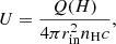
where Q(H) is the number of hydrogen-ionising photons emitted by the central source, and c is the speed of light. The intensity of the FUV radiation at the PDR front, G0, deduced in our Cloudy models, ranges from ∼17 to 11 481 in units of the Habing radiation field (1.6 × 10⁻³ ergs cm−2 s−1; Habing 1968). Five metallicity bins were calculated for the models: Z = 0.05, 0.1, 0.25, 0.5, and 1.0 Z⊙.
The dust and PAH properties used in this model are described in Cormier et al. (2019). The opacity curves of the SMC are used. The abundance of PAHs is further reduced by metallicity to the power of 1.3, characterising the prominent drop in PAH abundance at lower metallicity (e.g. Rémy-Ruyer et al. 2014, 2015). Tests performed in Cormier et al. (2019), inspecting the sensitivity of the PAH abundance, concluded that the PAH abundance is not an important factor in the outcome of the model results because the grain abundance is always larger than the already-reduced PAH abundance.
In Cloudy it is possible to choose a constant density throughout the cloud or to assume that the total pressure is constant. Cormier et al. (2019) looked into different approaches of the density law for a constant pressure case versus a constant density case and have found a compromise of these two extreme cases that works best in predicting the observations for the DGS sources. An intermediate case for the assumed density profile is constructed which is constant in the H II region and increases linearly with the hydrogen column density in the neutral gas. The different cases of constant density, constant pressure and smoothly-increasing density law were tested in Cormier et al. (2019) where, for example, the constant density models predict less [O I] emission and the constant pressure models predict more [O I] emission than the smoothly increasing density law adopted, which was found to successfully describe the observations.
A full galaxy has numerous stellar clusters and H II regions and ensembles of PDR/molecular clouds. To go from a model single cluster-plus-cloud system to a representation of a full galaxy with numerous cluster-plus-cloud systems, we create a “unit model” with total source luminosity = 109 L⊙. The unit model of 109 L⊙ chosen here is arbitrary but serves as a representative order of magnitude of luminosity of the observed galaxies. Thus all of the line luminosities predicted by the model correspond to a model for which L = 109 L⊙. The output masses are also determined for a model with source L = 109 L⊙. Since mass scales with luminosity, the masses determined for an individual galaxy, having LTIR (galaxy), are scaled by LTIR (galaxy)/109 L⊙. This approximation assumes an energy balance between UV-optical and IR and that LTIR scales similarly to the luminosity in the hydrogen-ionising energy range (Cormier et al. 2012). We refer to Cormier et al. (2019) for further details and input parameter studies of a similar model used for this study.
All Figures
|
Fig. 1. Comparison of a solar metallicity (metal-rich) molecular cloud and a low-metallicity cloud impacted by the UV photons of nearby star clusters. The decrease in dust shielding in the case of the low-metallicity cloud leads to further photodissociation of the molecular gas, leaving a layer of self-shielded H2 outside of the small CO-emitting cores. This CO-dark H2 can, in principle, be traced by [C II] or [C I]. |
| In the text | |
|
Fig. 2. LCO(1−0)/LFIR vs. L[C II]/LFIR observed in galaxies varying considerably in type, metallicity, and star formation properties. This is updated from Stacey et al. (1991, 2010), Madden (2000), and Hailey-Dunsheath et al. (2010) to include dwarf galaxies and more high-redshift galaxies. The dwarf galaxies are from Cormier et al. (2010, 2015) for the DGS; Grossi et al. (2016) for HeVICs dwarfs, and Smith & Madden (1997). High-redshift galaxies include those from Hailey-Dunsheath et al. (2010), Stacey et al. (2010), and Gullberg et al. (2015). The black and blue symbols are data from the original figure of Stacey et al. (1991) for Galactic star-forming regions, starburst nuclei and non-starburst nuclei, ULIRGS (Luhman et al. 2003), and normal galaxies (Malhotra et al. 2001). The dashed lines are lines of constant L[C II]/LCO(1−0). We note the location of the low-metallicity dwarf galaxies (red squares) that show extreme observed L[C II]/LCO(1−0) values. |
| In the text | |
|
Fig. 3. Evolution of the modelled gas parameters, Z, nH, and NH, as a function of depth (AV) for a solar-metallicity cloud (top left) and for a cloud of 0.1 Z⊙ (top right), with a starting density of 103 cm−3 and rin of 1020.7 cm, G0 = 380 in terms of the Habing field. Two central panels: effect of density variations (left: nH = 102 cm−3; right: nH = 104 cm−3) for Z = 0.5 Z⊙ with G0 = 380. Bottom two panels: effect of G0 variations (left: G0 = 80; right: G0 = 1800) for constant Z (0.5 Z⊙) and constant nH (103 cm−3). Each panel contains subpanels within, from top to bottom: cumulative mass in the ionised, neutral atomic, and molecular phases; normalised cumulative intensity of the [C II]λ158 μm, [C I]λ610 μm, and CO (1−0) lines; abundance of C+, C0, and CO relative to C; hydrogen density (nH) as a function of column density (NH) and AV; fraction of hydrogen in the ionised, atomic, and molecular form. The vertical dashed lines indicate the depth of the main phase transitions: H+ to H0, H0 to H2, CO(1−0) optical depth of 1. Masses indicated here should be adjusted for individual galaxies, scaling as LTIR (galaxy)/109 L⊙, as the source luminosity of the model is 109 L⊙ (see Appendix A). |
| In the text | |
|
Fig. 4. Grids of Cloudy calculations: model L[C II]/LTIR vs. H I and H2 mass reservoirs in the C+, C0-emitting regions, total H2 mass, and L[C II]/L[O I] behaviour (last column) in terms of metallicities of Z = 0.05, 0.1, and 1.0 Z⊙ (from top to bottom) and for a range of G0 and nH, the initial hydrogen density. The colour coding in each figure is log nH/cm−3 which increases from 1.0 (green) to 4.0 (purple). A range of G0 is set by varying log rin/cm from 21.3 at the top right of the grids (large dots) to 20.0 at the bottom left of the grids (smaller dots). These rin values cover a range of log G0 of 1.25 to 4.06 (Sect. 5). The Cloudy models are run with a source luminosity of 109 L⊙. Thus, the output masses should be scaled likewise (see Appendix A for details). The models are run to log N(CO)/cm−2 = 17.8 (AV ∼ 10 mag) for these grids. |
| In the text | |
|
Fig. 5. Model grids that provide the L[C II], L[C I](1−0) (609 μm), and LCO – to – MH2 conversion factors for Z = 1.0 Z⊙ (left) and Z = 0.1 Z⊙ (right) for the particular model using a cloud depth of log N(CO)/cm−2 = 17.8. The colour coding refers to density values ranging from log nH/cm−3 = 1 (green) to 4 (purple). G0 increases with increasing symbol size, taking values of 5, 20, 100, 200, and 500. To obtain the total molecular gas mass, which would include He, an additional factor of 1.36 (Asplund et al. 2009) should also be included for the total mass. We note that MH2 in the CO-emitting region is very sensitive to the depth at which the models are stopped which corresponds to AV ∼ 10 mag here. |
| In the text | |
|
Fig. 6. “Spaghetti plots”: model results for L[C II]/LCO(1−0) and ratios of LCO/MH2, L[C I]λ609 μm/MH2, and L[O I]/MH2 as a function of AV for a range of nH (101, 102, 103, 104 cm−3) and G0 values (∼20, 500, 8000) for Z = 0.05 Z⊙ (left) and 1.0 Z⊙ (right). |
| In the text | |
|
Fig. 7. Application of our model to the particular case of II Zw 40. Panels a show how the observed L[C II]/LTIR and L[C II]/L[O I] line ratios allow us to constrain nH and G0. Panel b shows how the L[C II]/LCO(1−0) ratio evolves in II Zw 40 as a function of AV, given the parameters previously derived from panel a. The green line indicates the best matching model. Panels c show the corresponding factors to convert L[C II], L[C I], and LCO to MH2 (see Sect. 6). |
| In the text | |
|
Fig. 8. Results from applying the models to the DGS sample and trends with model parameters. The vertical axis in panels a–c is M(H2)total/M(H2)CO (the ratio of the total MH2 determined from the model and the CO-bright MH2 determined from CO observations and the Galactic conversion factor) versus, on the horizontal axis, (a) G0, (b) density, and (c) AV. d: observed L[C II]/LCO(1−0) vs. model AV. Spearman correlation coefficients (ρ) and p-values in parenthesis are indicated within each panel. Red points are solutions for the DGS galaxies with CO detections. Open symbols are upper limits due to CO non-detections. The masses determined by the model for the individual galaxies have been scaled by their proper LTIR. |
| In the text | |
|
Fig. 9. Results for the DGS sample and trends with observable parameters. The vertical axis of panels a, c, d, and e is M(H2)total/M(H2)CO (total MH2 determined from the model over the MH2 determined from CO observations and the Galactic conversion factor). The horizontal axes of these same panels are as follows: a: L[C II]/LCO(1−0) with colour code for Z. The correlation shown in the dashed line is described in the panel in the equation for M(H2)total/M(H2)CO as a function of the observed L[C II]/LCO(1−0); standard deviation is 0.25 dex. b: total MH2 determined from the models vs. the observed L[C II]. Our resulting relationship of MH2 as a function of L[C II] is given within the panel; standard deviation is 0.14 dex. c: M(H2)total/M(H2)CO vs. Z; d: M(H2)total/M(H2)CO vs. observed L[C II]/LTIR. e: M(H2)total/M(H2)CO vs. ΣSFR, where SFR is determined from total IR luminosity from Rémy-Ruyer et al. (2015). Spearman correlation coefficients (ρ) and p-values in parenthesis are indicated within each panel. Red points are DGS galaxies with CO detections. Open symbols in all panels are upper limits due to CO non-detections. |
| In the text | |
|
Fig. 10. Consequences of quantifying the total H2 of the DGS sample. a: Schmidt–Kennicutt relationship and Bigiel et al. (2008) revisited. Solid black squares are the values when the MH2 is calculated from the CO-to-H2 standard conversion factor; solid red dots are the total H2 determined from our self-consistent models. The dashed line is the usual Schmidt–Kennicutt relation, where low-Z star-forming dwarf galaxies are normally outliers when CO is used to determine the H2 (Cormier et al. 2014). The dotted line is the Bigiel et al. (2008) relationship determined for the ΣSFR − Σgas relationship. b: αCO as a function of Z from Schruba et al. (2012; black dotted line), Glover & Mac Low (2011; long black dashed line), Accurso et al. (2017a; blue dashed line), Amorín et al. (2016; green dashed line), Genzel et al. (2015; short black dashed line), Tacconi et al. (2018; orange dashed line), Bolatto et al. (2013; pink dashed line), and our new αCO − Z relationship determined from this paper (red dashed line). Red solid dots are the total H2 determined from our self-consistent models in this paper. Also given in the panel is the derived expression to determine αCO as a function of Z from this new relationship, which has a standard deviation of 0.32 dex. c: XCO conversion factor from this paper and ΣSFR. Spearman correlation coefficients (ρ) and p-values in parenthesis are indicated within each panel. Red dots are DGS galaxies with CO detections. Open symbols in all panels are upper limits due to CO non-detections. |
| In the text | |
Current usage metrics show cumulative count of Article Views (full-text article views including HTML views, PDF and ePub downloads, according to the available data) and Abstracts Views on Vision4Press platform.
Data correspond to usage on the plateform after 2015. The current usage metrics is available 48-96 hours after online publication and is updated daily on week days.
Initial download of the metrics may take a while.