Alpha-element abundance patterns in star-forming regions of the Local Universe

C. Esteban; J. E. Méndez-Delgado; J. García-Rojas; K. Z. Arellano-Córdova; F. F. Rosales-Ortega; M. Orte-García; E. Reyes-Rodríguez; L. Carigi; A. Amayo

doi:10.1051/0004-6361/202453379

Home

All issues

Volume 697 (May 2025)

A&A, 697 (2025) A61

Full HTML

Open Access

Issue		A&A Volume 697, May 2025


Article Number		A61
Number of page(s)		22
Section		Interstellar and circumstellar matter
DOI		https://doi.org/10.1051/0004-6361/202453379
Published online		07 May 2025

A&A, 697, A61 (2025)

Alpha-element abundance patterns in star-forming regions of the Local Universe

C. Esteban¹^,2^★, J. E. Méndez-Delgado³, J. García-Rojas¹^,2, K. Z. Arellano-Córdova⁴, F. F. Rosales-Ortega⁵, M. Orte-García¹^,2, E. Reyes-Rodríguez¹^,2, L. Carigi³ and A. Amayo³

¹ Instituto de Astrofísica de Canarias, 38205 La Laguna, Tenerife, Spain
² Departamento de Astrofísica, Universidad de La Laguna, 38206 La Laguna, Tenerife, Spain
³ Instituto de Astronomía, Universidad Nacional Autónoma de México, Ap. 70-264, 04510 CDMX, Mexico
⁴ Institute for Astronomy, University of Edinburgh, Royal Observatory, Edinburgh EH9 3HJ, UK
⁵ Instituto Nacional de Astrofísica, Óptica y Electrónica (INAOE-CONAHCyT), Luis E. Erro 1, 72840 Tonantzintla, Puebla, Mexico

^★ Corresponding author: cel@iac.es

Received: 10 December 2024
Accepted: 21 March 2025

Abstract

Aims. We have undertaken a reassessment of the distribution of the alpha-element abundance ratios Ne/O, S/O, and Ar/O with respect to metallicity in a sample of about 1000 spectra of Galactic and extragalactic H II regions and star-forming galaxies (SFGs) of the Local Universe. We also analyse and compare different ionisation correction factor (ICF) schemes for each element in order to obtain the most confident determination of total abundances of Ne, S, and Ar.

Methods. We used the DEep Spectra of Ionised REgions Database (DESIRED) Extended project (DESIRED-E), comprising about 1000 spectra of H II regions and SFGs with direct determinations for the electron temperature (T_e). We homogeneously determined the physical conditions and chemical abundances for all the sample objects. We compared the Ne/O, S/O, and Ar/O ratios obtained using three different ICF schemes for each element. We also compared the abundance patterns with the predictions of a chemical evolution model of the Milky Way and stellar Ne and S abundance determinations.

Results. Following a careful analysis, we conclude that one of the tested ICF schemes provides a better match to the observed behaviour of Ne/O, S/O, and Ar/O ratios. We find that the distribution of Ne/O ratios in H II regions shows a large dispersion and no clear trend with O/H, indicating that the different ICF(Ne) schemes are not able to provide correct Ne/O ratios for most of these objects. This is not the case for SFGs, which show similar linear relations with slightly positive slopes for the distributions of log(Ne/O) with respect to 12+log(O/H) or 12+log(Ne/H). The origin of this abundance pattern may be the combination of a metallicity-dependent dust depletion of O and ICF effects. The log(S/O) versus 12+log(O/H) distribution is consistent with a constant value, especially for HII regions and when we consider both types of objects (SFGs + H II regions). However, the log(S/O) versus 12+log(S/H) distribution shows a rather tight linear fit with a positive slope. This relation seems to flatten at 12+log(S/H) ≲ 6.0. We find that the observed behaviour of S/O with S/H is compatible with some contribution of S produced by Type Ia supernovae (SNe Ia). Finally, the behaviour of log(Ar/O) versus 12+log(O/H) is very similar for H II regions and SFGs and seems to be independent of the ionisation degree and the type of ICF(Ar) used, no matter whether it is based on only the ([Ar III] lines or on the combination of [Ar III] and [Ar IV] lines. The linear fit to log(Ar/O) versus 12+log(O/H) indicates a slight decrease in log(Ar/O) as 12+log(O/H) increases. However, the log(Ar/O) versus 12+log(Ar/H) relation shows an inverse trend, with a small positive slope that could indicate a small contribution of Ar from SNe Ia.

Key words: nuclear reactions, nucleosynthesis, abundances / ISM: abundances / HII regions / galaxies: abundances

© The Authors 2025

Open Access article, published by EDP Sciences, under the terms of the Creative Commons Attribution License (https://creativecommons.org/licenses/by/4.0), which permits unrestricted use, distribution, and reproduction in any medium, provided the original work is properly cited.

This article is published in open access under the Subscribe to Open model. Subscribe to A&A to support open access publication.

1 Introduction

The analysis of emission line spectra of star-forming regions is the main source of information on the chemical composition of the Universe and its evolution over cosmic time. Using standard tools for analysing ionised nebulae in the optical, ultraviolet, and infrared spectral ranges, we can determine the chemical abundances of an important fraction of the most abundant elements, such as He, C, N, O, Ne, S, Cl, Ar, Fe, and Ni. Among these, only O shows bright optical emission lines from all of its possible ionisation states most common in star-forming regions. Therefore, the total O abundance is usually simply the sum of the ionic abundances of its observed ionisation states (solely O⁺ and O²⁺). In addition to the ease of determining its abundance from nebular spectra, O is the third most abundant chemical element in the Universe, which explains why it is used as a proxy for metallicity in the ionised gas-phase of the interstellar medium (ISM). For the remaining elements apart from O, we need to use an ionisation correction factor (ICF) to estimate their total abundances (e.g. Peimbert & Costero 1969; Peimbert & Torres-Peimbert 1977; Stasińska 1978; Mathis 1985; Izotov et al. 2006; Pérez-Montero et al. 2007; Dors et al. 2013, 2016; Amayo et al. 2021). These ICFs allow us to estimate the contribution of unseen ionisation states to the total abundance of a given element.

Oxygen is produced in hydrostatic nucleosynthesis in the interior of massive stars (>8 M_⊙) after the triple-alpha process, where helium is fused into C and other heavier elements during the final stages of stellar evolution. It is then further produced and finally released into the ISM during the stellar wind phase and explosion of the dying star as core-collapse supernovae (CCSNe) on short timescales (e.g. Woosley et al. 2002; Chiappini et al. 2003; Limongi & Chieffi 2018; Kobayashi et al. 2020). The so-called alpha elements are those lighter than Fe, whose mass number of their most abundant isotope is a multiple of 4, that is, they contain an integer number of alpha particles or He nuclei. Ne, S, and Ar are alpha elements and, in principle, they should have the same nucleosynthetic origin as O and therefore present a similar behaviour in their cosmic evolution (e.g. Izotov et al. 2006; Croxall et al. 2016; Esteban et al. 2020; Rogers et al. 2022; Arellano-Córdova et al. 2024). As a result, the abundance ratio of any of these alpha elements with respect to O should remain constant. However, some nucleosynthesis and chemical evolution models predict some contribution of S and Ar from type I supernovae (SNIa, e.g. Iwamoto et al. 1999; Johnson 2019; Kobayashi et al. 2020). When applying those models, a certain deviation (i.e. a slight increase) in the S/O and Ar/O ratios with respect to O/H – but also with respect to S/H and Ar/H – would be expected. Whether or not the abundance ratio of alpha-elements with respect to O is constant is not yet a well-established issue from an observational point of view. The analysis of emission-line spectra of ionised nebulae is the main source of information on the abundances of Ne, S, and Ar in the cosmos. In particular, for Ar it is the only possibility, since there are no lines of this element in stellar spectra. The situation for Ne is not so unfavorable, although it is only possible to obtain Ne abundances in the spectra of O and B-type stars.

In the Local Universe, most studies devoted to chemical abundances in the ionised gas contained in star-forming regions find that Ne/O, S/O, and Ar/O ratios do indeed remain basically constant with the metallicity of the gas, considering the rather large statistical dispersion and observational errors (e.g. Kennicutt et al. 2003; Izotov et al. 2006; Arellano-Córdova et al. 2020, 2024; Berg et al. 2020; Rogers et al. 2022). Yet there is no shortage of works that argue the presence of some trends, at least for some alpha-elements. In the case of S/O, Díaz & Zamora (2022) find that it decreases significantly as metallic-ity increases but only when the star-forming galaxies (SFGs) are removed from their sample. In the case of Ar, Arnaboldi et al. (2022) report an increase of the Ar/O ratio as the Ar/H increases from the spectra of a sample of planetary nebulae in the M31 galaxy, a behaviour they have interpreted as the effect of Ar production by SNe Ia. On the other hand, Izotov et al. (2006), Pérez-Montero et al. (2007), Kojima et al. (2021), and Miranda-Pérez & Hidalgo-Gámez (2023) found the opposite trend for Ar/O, but only when limited or particular samples of objects are considered. In principle, the situation should be clearer in the case of Ne, as the models predict that its nucleosynthesis mechanisms are essentially the same as those for O, however, there is also no lack of indications that the Ne/O ratio may not be constant. Izotov et al. (2006) observed a slight increase in Ne/O of about 0.1 dex over the entire metallicity range – 12+log(O/H) from 7.1 to 8.6 – of their sample of SFGs. They attributed this feature to moderate depletion of O onto dust grains in their most metal-rich objects. On the other hand, although the results obtained by Croxall et al. (2016) for H II regions are consistent with a basically constant value, they also find a population of objects with a significant offset to low Ne/O ratios. The calculation of the total abundance of Ne comes with the problem that its ionisation corrections are less well constrained than in the case of other elements, so some of the reported trends may depend on the ionisation degree of the objects and therefore be ultimately an effect of the ICF used (e.g Kennicutt et al. 2003; Berg et al. 2020; Arellano-Córdova et al. 2024).

In recent years, and especially with the advent of the James Webb Space Telescope (JWST), metallicity determinations from the analysis of emission line spectra have started to be obtained for high-z SFGs (e.g. Arellano-Córdova et al. 2022; Schaerer et al. 2022; Brinchmann 2023; Curti et al. 2023; Isobe et al. 2023; Nakajima et al. 2023). Even in some objects, the detection of the faint auroral [O III] λ4363 line has permitted to determine the electron temperature, T_e , and to apply the so-called direct method (Dinerstein 1990; Peimbert et al. 2017) to obtain more precise determinations of the O abundance (e.g. Arellano-Córdova et al. 2022; Schaerer et al. 2022; Curti et al. 2023; Rhoads et al. 2023; Trump et al. 2023; Laseter et al. 2024). The total abundances of Ne, S, and Ar have been determined for several SFGs at z = 4–10, offering the opportunity to study the evolution of the Ne/O, S/O, and Ar/O abundance ratios over cosmic time (e.g. Arellano-Córdova et al. 2022; Isobe et al. 2023; Marques-Chaves et al. 2024; Stanton et al. 2025). In the case of Ne, Arellano-Córdova et al. (2022, 2024), Isobe et al. (2023), and Stanton et al. (2025) found that the Ne/O ratio (when comparing its behaviour with that of the Local Universe) does not appear to evolve with redshift. However, on the other hand, Stanton et al. (2025) found evidence of evolution of the Ar/O ratio with redshift.

To properly analyse the growing amount of data on the chemical content of high-z SFGs, it is of utmost importance to have high-quality chemical abundance data for a representative sample of objects in the Local Universe for comparison. For example, Izotov et al. (2006) presented the Ne/O, S/O, and Ar/O abundance ratios for a sample of about 400 SFGs. Pérez-Montero et al. (2007) recalculated abundances for 633 SFGs and 220 H II regions. More recent studies, as that of Berg et al. (2020), present O, N, Ne, S, and Ar abundance data for 190 individual H II regions in four spiral galaxies. Another recent large study was recently published by Díaz & Zamora (2022), who presented O and S abundances for 256 H II regions and 95 SFGs.

The main aim of this work is to make a reassessment of the analysis of Ne/O, S/O, and Ar/O abundance ratios by making use of the largest possible sample of high quality spectra from local H II regions and SFGs. For this dataset, we recalculated the precise abundances, using the direct method and applying the methodology developed by our group in a homogeneous manner. The characteristics of this sample, collected in the DEep Spectra of Ionised REgions Database (DESIRED) project (Méndez-Delgado et al. 2023a) are described in Sect. 2. Another aim of this work is to compare the total abundances of Ne, S, and Ar obtained using different ICF schemes to select those that show a more independent behaviour with respect to the ionisation degree. In this way, we try to get a closer look at the actual behaviour of the Ne/O, S/O, and Ar/O ratios with respect to metallicity in the Local Universe.

2 Description of the sample of H II regions and star-forming galaxies

The present work is part of the DESIRED project (Méndez-Delgado et al. 2023a) dedicated to the homogeneous analysis of optical spectra of ionised nebulae. The nucleus of DESIRED is comprised by a set of almost 200 deep intermediate- and high-spectral-resolution spectra of Galactic and extragalactic H II regions, SFGs, Galactic planetary nebulae (PNe) and ring nebulae (RNe) around evolved massive stars, as well as a small number of Herbig-Haro objects and protoplanetary discs of the Orion Nebula, observed by our research group over the last 20 years. In addition to the former DESIRED objects, we decided to include additional high-quality spectra of H II regions, SFGs, and PNe from the literature having direct determination of Te. We refer to this larger sample as DESIRED Extended (DESIRED-E) and it currently contains 2133 spectra as of July 25, 2024. We use this spectra dataset in the present study.

A first description of DESIRED-E and the format of the datafiles can be found in Méndez-Delgado et al. (2024). For each spectra, we compiled the extinction-corrected intensity ratios (along with their corresponding uncertainties) of all the emission lines reported in the reference papers. In all the cases, we only considered the line ratios whose quoted observational errors were less than 40%. In this paper, we focus our attention on the study of the abundance ratios of alpha elements, limiting our abundance calculations to O, Ne, S, and Ar in Galactic and extragalactic H II regions (designated simply as ‘H II regions’) and SFGs of DESIRED-E. The extragalactic H II regions comprise individual star-forming nebulae in spiral or irregular galaxies and SFGs correspond to dwarf starburst galaxies, whose general spectroscopic properties are indistinguishable from giant extragalactic H II regions (e.g. Sargent & Searle 1970; Melnick et al. 1985; Telles et al. 1997).

All H II regions and SFGs of DESIRED-E have at least one detection of the following auroral or nebular intensity ratios of collisionally excited lines (CELs): [O III] λ4363/λ5007, [N II] λ5755/λ6584, and [S III] λ6312/λ9069. With these line ratios, we can derive T_e values that are insensitive to values of the electron density, ne, of the order or lower than 10⁴ cm⁻³ (Froese Fischer & Tachiev 2004; Tayal 2011). It is widely known that a good determination of T_e is necessary to obtain reliable values of ionic abundances from the intensity of CELs. All DESIRED-E objects have direct determinations of the total O abundance (the proxy of metallicity in ionised nebulae studies) and they cover a range of 12+log(O/H) values from 6.9 to 8.9 approximately. In Fig. 1 we show the position of the H II regions and SFGs compiled in DESIRED-E in the Baldwin-Phillips-Terlevich (BPT) diagram (Baldwin et al. 1981). Objects located above or at the right of the Kauffmann et al. (2003) line have not been considered in the calculations. Those discarded objects have hard ionising sources that can be associated with an active galactic nucleus (AGN) and/or can be affected by shock excitation as in some RNe around Wolf–Rayet stars (e.g. Esteban et al. 2016). We applied additional filters (see Fig. 1) to exclude objects that, due to their position on the BPT diagram, were not considered in the ionisation models used by Amayo et al. (2021) to construct their set of ionisation correction factors (ICFs). This is one of the sets of ICFs that we use to determine the total abundances of Ne, S, and Ar, as we explain in Sect. 4. The application of the additional filters of Amayo et al. (2021) only involves the rejection of around 2% of the objects. The total number of DESIRED-E spectra classified as H II regions or SFGs that fulfill our filters in the BPT diagram is 1829, with 43.0% corresponding to H II regions and 57.0% to SFGs. From this initial sample, we selected 1386 objects for which we were able to determine the total abundance of one, two, or three of the alpha elements (Ne, S, and Ar) that is detectable in the nebular optical spectra.

In Table D.2 we list the 1386 objects included in the present study, indicating their name, whether they correspond to H II regions or SFGs, both types correspond exactly to 50% of the objects by a happy coincidence. We also give the reference pertaining to their published spectra.

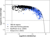Fig. 1

BPT diagram of the sample of spectra of Galactic and extragalactic H II regions and SFGs compiled in DESIRED-E. The dashed line represents the empirical relation by Kauffmann et al. (2003) that distinguishes between star-forming regions and AGNs. The dotted vertical and horizontal lines represent additional filters applied by Amayo et al. (2021) to photoionisation models to construct their set of ICFs.

3 Physical conditions and ionic abundances

We made use of PyNeb 1.1.18 (Luridiana et al. 2015; Morisset et al. 2020)¹ with the atomic dataset presented in Table D.1 and the H I effective recombination coefficients from Storey & Hummer (1995) to determine the physical conditions and the ionic abundances of the ionised nebulae. PyNeb is written in Python programming language and is fully vectorised. To calculate the emissivity of collisional excitation lines, PyNeb calculates the relative population of the atomic levels of the ions of interest by solving the statistical equilibrium equations. In the case of recombination lines, it interpolates the available emissivity tables.

3.1 Physical conditions

We used the getCrossTemDen routine of PyNeb with line intensity ratios sensitive to n_e and T_e . We crosscorrelated the density-sensitive diagnostics [S II] λ6731/ λ6716, [O II] λ3726/λ3729, [Cl III] λ5538/λ5518, [Fe III] λ4658/λ4702, and [Ar IV]λ4740/λ4711 with the temperaturesensitive ones [N II] λ5755/λ6584, [O III] λ4363/λ5007, [Ar III] λ5192/λ7135, and [S III] λ6312/λ9069 using a Monte Carlo experiment and generating 100 random values to propagate uncertainties in line intensities. This number was chosen as a compromise between calculation time and convergence of the result. With this procedure, we obtained a set of ne and Te values and their associated uncertainties for each diagnostic and individual point of the experiment. The average n_e, weighted by the inverse square of the error of the 100 individual points, was adopted as the representative value of the diagnostic. This procedure enabled us to take into account the small temperature dependence of density diagnostics under typical nebular conditions, which is not considered in many works in the literature.

Once we obtained the density for each diagnostic, we applied the criteria proposed by Méndez-Delgado et al. (2023a) to estimate an average density representative of each nebulae. If ne([S II] λ6731/λ6716) < 100 cm⁻³, we adopted n_e = 100±100 cm⁻³. If 100 cm⁻³ ≤ n_e([S II] λ6731/λ6716) <1000 cm⁻³, we adopt the average between n_e([S II] λ6731/λ6716) and n_e([O II] λ3726/λ3729). If n_e([S II] λ6731/λ6716) ≥ 1000 cm⁻³, we adopted the average of n_e([S II] λ6731/λ6716), n_e([O II] λ3726/λ3729), n_e([Cl III] λ5538/λ5518), n_e([Fe III] λ4658/λ4702), and n_e([Ar IV] λ4740/λ4711). In cases where a value of n_e was not reported or could not be calculated in the source references, we adopted n_e = 100±100 cm⁻³.

We estimated the temperatures T_e([N II] λ5755/λ6584), T_e([O III] λ4363/λ5007) and T_e([S III] λ6312/λ9069) using the getTemDen routine of PyNeb and the aforementioned average n_e of each object. We also used a Monte Carlo experiment of 100 random values to propagate uncertainties in n_e and line intensity ratios to estimate the error of each T_e diagnostic. To ensure a good determination of T_e for each object, we excluded all determinations of auroral lines with errors greater than 40% and verified that the flux of the pairs of nebular lines coming from the same upper atomic level used (e.g., [O III] λλ5007, 4959, [S III] λλ9531, 9069, and [N II] λλ6584, 6548) fit with their theoretical predictions, regardless of the physical conditions of the gas (Storey & Zeippen 2000). We discarded any diagnostic when the observed nebular line intensity ratios differ by more than 20% from the theoretical ones. Departures from the theoretical case are rather common in the case of [S III] λλ9531, 9069, due to the contamination of telluric absorption bands (see Méndez-Delgado et al. 2024, for a discussion of this issue). There is a small number of objects where only one of the lines of the aforementioned pairs of nebular lines is reported. In these cases, we consider the single nebular line observed in the calculation, assuming that the T_e derived is valid. In this paper, we only adopted T_e([S III]) to determine ionic abundances in the absence of T_e([N II]) and T_e([O III]). We give our derived physical conditions in Table D.3.

3.2 Ionic abundances

We determined the ionic abundances of O⁺, O²⁺ , S⁺, S²⁺, Ne²⁺, Ar²⁺, and Ar³⁺. For O⁺, we used the [O II] λλ3727, 3729 doublet and the sum of the auroral lines [O II] λλ7319, 7320, 7330, 7331 when the bluer [O II] doublet lines were not available. In the case ofO²⁺, we used the sum of the bright [O III] λλ4959, 5007 nebular lines. For S⁺ and S²⁺, we used the sum of [S II] λλ6716, 6731 and [S III] λλ9069, 9531 doublets, respectively. There are spectra that do not cover the near-IR range, so in such cases we used the [S III] λ6312 line to derive the S²⁺ abundance. For Ne²⁺, we used the [Ne III] λ3868 line because [Ne III] λ3967 is usually blended with H I λ3970 in most of the spectra. In the case of Ar²⁺, we used the [Ar III] λ7136 line alone or in combination with [Ar III] λ7751 when both lines were available. Finally, we used the [Ar IV] λλ4711, 4740 doublet to derive the Ar³⁺ abundance. We note that the He I λ4713 line may contaminate [Ar IV] λ4711 in the low-resolution spectra of high-ionisation objects, especially in SFGs. As we explain in Sect. 4.3, there is no indication of a significant sample of objects with abnormally high Ar/O ratios that might be affected by this problem.

We assumed T_e([N II] λ5755/λ6584) and the adopted value of n_e in the getIonAbundance routine of PyNeb to calculate the abundance of the low-ionisation ions O⁺ and S⁺, propagating the uncertainties in n_e, T_e and the line ratios through 100-point Monte Carlo experiments. When T_e([N II] λ5755/λ6584) was not available for a given spectrum, we applied the temperature relations of Garnett (1992) to estimate it from T_e([O III] λ4363/λ5007), or T_e([S III] λ6312/λ9069) when the first diagnostic was also absent. The O²⁺, Ne²⁺, and Ar³⁺ abundances are determined using T_e([O III] λ4363/λ5007) and the adopted value of n_e . In the spectra where T_e([O III] λ4363/λ5007) was not available, we used the temperature relations of Garnett (1992) along with the values of T_e([N II] λ5755/λ6584) and/or T_e([S III] λ6312/λ9069) when one of these are determined from the spectra. The abundance of the intermediate-ionisation ions, S²⁺ and Ar²⁺ , is calculated using the adopted value of n_e and T_e([S III] λ6312/λ9069), T_e([N II] λ5755/λ6584), or T_e([O III] λ4363/λ5007), along with the temperature relations of Garnett (1992) when T_e([S III] λ6312/λ9069) was not available. The ionic abundances of O⁺, O²⁺, S⁺, S²⁺, Ne²⁺, Ar²⁺, and Ar³⁺ of the objects included in this study are shown in Table D.4.

4 Total O, Ne, S, and Ar abundances

The total O abundances were calculated as the sum of the O⁺/H⁺ and O²⁺/H⁺ ratios. The contribution of O³⁺/H⁺ to the total O/H ratio was not considered, as observational studies of metal-poor regions (e.g. Izotov & Thuan 1999; Berg et al. 2021; Domínguez-Guzmán et al. 2022) have found small values up to the order of 5% (0.02 dex at maximum) that can be considered negligible compared to the typical errors of the O/H ratio.

As stated in Sect. 1, we have to consider ICFs to determine the total abundances of Ne, S, and Ar. Following a philosophy similar to that of previous works in H II regions and SFGs (e.g. Arellano-Córdova et al. 2020, 2024), we compared the elemental abundances and their ratios obtained using different correction schemes to achieve the most model-independent and robust total abundance determinations possible. For each element, we compared and analysed the results using three ICF schemes. Two of them, namely those of Amayo et al. (2021) and Izotov et al. (2006), are common to Ne, S, and Ar, while the third scheme is different for each element; Dors et al. (2013) for Ne, Dors et al. (2016) for S, and Pérez-Montero et al. (2007) for Ar. In Fig. A.1, we include the differences between the Ne, S, and Ar abundances (in logarithmic form) obtained for the spectra of the DESIRED-E sample using the different ICF schemes. The shapes of the curves help to interpret the distribution of abundance ratios that will be discussed below. Moreover, the range of values covered by the observational points in these figure (which depends on the element, the emission lines used, and the degree of ionisation) gives us an idea of the uncertainty introduced by the use of an ICF on the value of the total abundance of a given element and object.

4.1 Neon

Overall, Ne²⁺ is the only ionisation state of Ne that presents emission lines in the optical range of the spectrum. UV photons with energies between 41.0 and 63.5 eV can produce Ne²⁺; therefore, we expect an important fraction of unobservable Ne⁺ to be present in typical star-forming ionised nebulae. To obtain the Ne/O ratio, we apply the relation:

$\frac{Ne}{O} = \frac{{Ne}^{2 +}}{O^{2 +}} \times ICF(Ne) .$ $\frac{\text{Ne}}{\text{O}} = \frac{\text{Ne}^{2+}}{\text{O}^{2+}} \times \text{ICF(Ne)}.$ (1)

As indicated previously, we used three different ICF(Ne)² schemes to derive the total Ne abundance. The set by Amayo et al. (2021) is based on a grid of photoionisation models from the Mexican Million Models data base (3MdB Morisset 2009) under the ‘BOND’ reference (Vale Asari et al. 2016). This grid was selected by applying several filters to resemble the properties of a large observational sample of extragalactic H II regions and the integrated spectra of SFGs. For their ionisation models, Amayo et al. (2021) adopted stellar spectral energy distributions (SEDs) obtained with the PopStar code (Mollá et al. 2009). All the ICFs of Amayo et al. (2021) used in this study depend on the mean ionisation degree of the nebulae (parameterized by the O²⁺/O ratio) and they are, in principle, valid for the whole range of ionisation degrees. The second ICF(Ne) scheme we used is that from Izotov et al. (2006), who used the grid of photoionisation models of SFGs presented by Stasiń ska & Izotov (2003) and input stellar SED models from Starburst99 (Leitherer et al. 1999). The ICFs by Izotov et al. (2006) depend on the ionisation degree and the metallicity. They propose different equations for ‘low’ (12+log(O/H) ≤ 7.2), ‘intermediate’ (7.2 < 12+log(O/H) < 8.2), and ‘high’ (12+log(O/H) ≥ 8.2) metallicity that are used to interpolate the appropriate value of the ICF using the O/H ratio of the object. In the case of the ICF(Ne), the relations given by Izotov et al. (2006) are valid for any value of the O²⁺/O ratio. The last ICF(Ne) scheme considered in this study is that by Dors et al. (2013), which is based on photoionisation models of extragalactic H II regions and SFGs that use ionising SEDs from Starburst99 (Leitherer et al. 1999). They have provided an analytical expression (their Eq. (14), applicable for data obtained from optical spectra) parameterised by the O²⁺/O ratio and valid for all the range of ionisation degrees.

In the top panel of Fig. 2, we plot log(Ne²⁺/O²⁺) as a function of O²⁺/O for 557 spectra of H II regions and 671 of SFGs of the DESIRED-E sample (1228 in total). The coloured curves represent the different ICF(Ne) values defined by Eq. (1) provided by each of the ICF schemes considered: Amayo et al. (2021, shown as red dashed-dotted lines), Izotov et al. (2006, shown as dotted lines with colours corresponding to the three metallicity ranges,) and Dors et al. (2013, shown as the green dashed line). The horizontal black dashed line indicates the solar log(Ne/O) of −0.63 ± 0.06 along as its uncertainty represented by the grey band, taken from Asplund et al. (2021); this line also represents the classical ICF of Peimbert & Costero (1969), that assumes Ne²⁺/O²⁺ = Ne/O. Figure 2 clearly indicates that the dispersion of the log(Ne²⁺/O²⁺) values of objects classified as H II regions is much larger than the dispersion of those classified as SFGs. This observational fact was reported by Kennicutt et al. (2003) and Croxall et al. (2016), among others. Figure 2 also shows that the ICF(Ne) by Amayo et al. (2021) seems to better reproduce the behaviour oflog(Ne²⁺/O²⁺) for objects with O²⁺/O < 0.5 (mostly H II regions), but giving fairly higher values of log(Ne/O) (between 0.1 and 0.3 dex higher) than the ICF(Ne) schemes by Izotov et al. (2006) and Dors et al. (2013) in the whole ionisation range. This can be noted very clearly in the different distribution of the blue and magenta points in the top left panel of Fig. A.1. The Ne abundances obtained using the different ICFs can differ by up to 0.3 dex when O²⁺/O < 0.5, although this difference decreases at higher ionisation degrees, reaching values below 0.1 dex when O²⁺/O > 0.8.

In Fig. 3, we show the log(Ne/O) values obtained with the three ICF(Ne) schemes we used to derive the total Ne abundance for our DESIRED-E objects. We represent log(Ne/O) as a function of 12+log(O/H) (left panels) and O²⁺/O (right panels). We can derive the Ne abundances for a total number of 1228 spectra, with 45.4% of them corresponding to H II regions and 54.6% to SFGs. In the figure, we can note that in most panels, the distribution of the points show systematic trends that move away from a line of constant value, which is in contradiction with be expected behaviour for two elements with similar nucleosynthetic origin as it is thought to be the case of Ne and O. To better illustrate the behaviour of log(Ne/O), we represent its mean value for several bins (orange diamonds) in the areas of the figures having a significant number of points (more than 10), for values of 12+log(O/H) from 7.0 to 9.1 (bins 0.30 dex wide) and for O²⁺/O values from 0.1 to 1.0 (bins 0.15 wide).

The two top panels of Fig. 3 show the log(Ne/O) values obtained with the ICF(Ne) by Amayo et al. (2021). The upper left panel shows a rather slight increase of log(Ne/O) with respect to the O abundance. In fact, the bin corresponding to the highest 12+log(O/H) values has a mean log(Ne/O) 0.05 dex higher than the bin containing the objects with lowest O abundances. On the other hand, in the upper right panel, the data points are distributed following a curved distribution with a convex shape (looking from positive ordinates), with an amplitude of variation of log(Ne/O) of about 0.17 dex along the whole O²⁺/O range. The ICF(Ne) of Amayo et al. (2021) tends to give oversolar log(Ne/O) values, in fact the mean log(Ne/O) obtained from all the data points is −0.55 ± 0.12, larger than the solar value of −0.63 ± 0.06 (Asplund et al. 2021), although still consistent within the errors.

In the two middle panels of Fig. 3, we present the log(Ne/O) values obtained using the ICF(Ne) scheme by Izotov et al. (2006). It can be seen that the log(Ne/O) versus 12+log(O/H) distribution is somewhat flatter in this case, log(Ne/O) tends to decrease in about 0.03 dex from lowest to highest metallicities. However, it is clear that the ICF(Ne) scheme by Izotov et al. (2006) does not correct appropriately for the presence of Ne⁺ in objects with O²⁺/O < 0.5. The difference between the bins at the extremes is ∼0.19 dex. The ICF(Ne) by Dors et al. (2013) shows a similar trend in the log(Ne/O) versus O²⁺/O panel, but with a more pronounced difference between the bins at the extremes (∼0.37 dex). The bottom left panel of Fig. 3 illustrates that the ICF(Ne) by Dors et al. (2013) produces a decrease of log(Ne/O) as the metallicity increases, with a difference of about 0.15 dex between the bins at the extremes of the 12+log(O/H) range. The ICF(Ne) by Izotov et al. (2006) and Dors et al. (2013) give mean values of the Ne/O ratio of −0.67 ± 0.12 and −0.68 ± 0.13, respectively; this is below (but still in agreement with) the solar value of −0.63 ± 0.06 (Asplund et al. 2021).

Figure 3 illustrates that all the ICF(Ne) schemes considered fail to give correct Ne/O ratios for nebulae having O²⁺/O ≤ 0.5, that would correspond mainly to intermediate and high-metallicity objects. The vast majority of the objects of the DESIRED-E sample in that part of the log(Ne/O) versus O²⁺/O diagram correspond to H II regions. In fact, as this is an expected result according to the behaviour of the ICF(Ne) curves against the observed distribution of the Ne²⁺/O²⁺ ratios of the DESIRED-E objects shown in the upper panel of Fig. 2 The total O and Ne abundances determined using the different ICF schemes considered – as well as the total abundances of S and Ar – are collected in Table D.5.

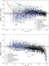Fig. 2

Log(Ne²⁺/O²⁺) (top) and log((S⁺ +S²⁺)/O) (bottom) as a function of the ionisation degree, O²⁺/O, for DESIRED-E sample of H II regions (blue circles) and SFGs (black squares). The black dashed lines and the grey bands show the solar log(Ne/O) and log(S/O) values and their associated uncertainty, respectively, from Asplund et al. (2021). The different curves represent the ICF schemes used in this study: Amayo et al. (2021, shown as red dashed-dotted lines), Izotov et al. (2006, shown as dotted lines with colours corresponding to three metallicity ranges), Dors et al. (2013, shown as the green dashed line in top panel,) and Dors et al. (2016, shown as the green dashed line in the bottom panel).

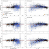Fig. 3

log(Ne/O) as a function of 12+log(O/H) (left) and the ionisation degree, O²⁺/O (right), for the DESIRED-E sample of H II regions (blue circles) and SFGs (black squares). Panels in the same row represent log(Ne/O) calculated using the ICF(Ne) scheme of Amayo et al. (2021, top panels), Izotov et al. (2006, middle panels), and Dors et al. (2013, bottom panels). The dotted red line represents the mean value of the log(Ne/O) obtained using each ICF(Ne). The orange diamonds indicate the mean log(Ne/O) values considering bins in 12+log(O/H) or O²⁺/O. The black dashed lines and the grey bands show the solar 12+log(O/H) and log(Ne/O) and their associated uncertainties, respectively, from Asplund et al. (2021).

4.2 Sulfur

Sulfur presents bright emission lines of S⁺ and S²⁺ in the optical spectra of ionised nebulae. S⁺ can be ionised by photons with energies between 10.4 to 22.3 eV and S²⁺ from 22.3 to 34.8 eV. Therefore, we expect a certain fraction of S³⁺ (34.8– 47.2 eV) to be present under the typical ionisation conditions of H II regions and SFGs. In many nebular spectra of faint objects only [S II] lines can be observed, so the only possibility to derive their total S/H is from the S⁺ abundance. Amayo et al. (2021) obtained an expression for an ICF(S) based only on the intensity of [S II] lines but they find large differences and uncertainties with respect to the values obtained using [S II] and [S III] lines. Therefore, Amayo et al. (2021) did not recommend to use an ICF(S) based on S⁺ alone. Considering this, we only obtain the S/O ratio for those objects for which we can derive both, S⁺ and S²⁺ abundances. We can apply the following relation (see footnote in Sect. 4.1):

$\frac{S}{O} = (\frac{S^{+} + S^{2 +}}{O}) \times ICF(S) .$ $\frac{\text{S}}{\text{O}} = \left(\frac{\text{S}^{+}+\text{S}^{2+}}{\text{O}}\right) \times \text{ICF(S)}.$ (2)

We used three different ICF(S) schemes to derive the S abundance. The first two are the same that we use in the case of Ne, the sets by Amayo et al. (2021) and Izotov et al. (2006), described in Sect. 4.1. The third ICF(S) scheme is the one proposed by Dors et al. (2016), based – as in the case of the ICF(Ne) by Dors et al. (2013) described in Sect. 4.1– on photoionisation models for extragalactic H II regions and SFGs using ionising SEDs from Starburst99. The values of the IFC(S) provided by the three schemes are parameterized by the O²⁺/O ratio. The ICF(S) by Amayo et al. (2021) and Dors et al. (2016) are valid for all the range of ionisation degrees, but the one by Izotov et al. (2006) can only be applied for objects with O²⁺/O ≥ 0.2.

In the bottom panel of Fig. 2, we plot log((S⁺+S²⁺)/O) as a function of the ionisation degree, O²⁺/O, for 509 H II regions and 493 SFGs of the DESIRED-E sample with measurements of both, [S II] and [S III] lines. The coloured curves represent the behaviour of the different ICF(S) schemes considered: Amayo et al. (2021, shown as red dashed-dotted lines), Izotov et al. (2006, shown as dotted lines with colours corresponding to the three metallicity ranges,) and Dors et al. (2016, shown as the green dashed line). The horizontal black dashed line shows the value of the solar log(S/O) ratio, along as its uncertainty represented by the grey band, recommended by Asplund et al. (2021). Figure 2 shows that from values of O²⁺/O larger than about 0.5, the contribution of S³⁺ in the nebulae (with an IP of 34.8 eV) becomes important. In the figure we can see that only the ICF(S) scheme by Izotov et al. (2006) reproduces the observed log((S⁺+S²⁺)/O) values for very high ionisation degree objects (with O²⁺/O ≥ 0.9), mostly corresponding to SFGs.

In Fig. 4, we show the log(S/O) values obtained with the three ICF(S) schemes we use to derive the total S abundance for the DESIRED-E spectra. The exact number depends on the ICF(S) scheme used, 1002 with Amayo et al. (2021) or Dors et al. (2016) (50.8% H II regions and 49.2% SFGs) and 933 with Izotov et al. (2006, 47.2% H II regions and 52.8% SFGs). Similarly to Fig. 3 for log(Ne/O), in Fig. 4 we represent log(S/O) as a function of 12+log(O/H) and O²⁺/O. In the right panels of Fig. 4, we can note that the distribution of the sample points using the ICF(S) by Amayo et al. (2021) and Dors et al. (2016) show a systematic tendency to give lower log(S/O) values as the ionisation degree of the objects increases. The mean log(S/O) corresponding to the different O²⁺/O bins decreases almost monotonically 0.30 and 0.27 dex, respectively for the two aforementioned ICF(S) schemes along the whole range of O²⁺/O ratios. This trend: (a) clearly indicates that the ICF(S) by Amayo et al. (2021) and Dors et al. (2016) do not completely correct for the ionisation dependence the conversion from the sum of the ionic abundances to the final S/H ratio; (b) can also explain, at least partially –due to the rough relation between O/H and O²⁺/O (see Fig. B.1) –, the increase in log(S/O) as a function of 12+log(O/H) that can be seen in the top and bottom panels on the left columns of Fig. 4. The 12+log(O/H) bins plotted in both panels show a systematic increase of +0.17 dex in log(S/O) as the metallicity increases.

The two panels of the middle row of Fig. 4 show the results using the ICF(S) by Izotov et al. (2006), which clearly provides flatter trends than the other schemes. In fact, the maximum variation between the extreme values of the log(S/O) of the bins represented in both panels is only of the order of 0.1 dex. Another argument to claim that the ICF(S) by Izotov et al. (2006) is more appropriate is the shortage of objects with very low log(S/O) at O²⁺/O ≥ 0.95, which appears when the other two IFC(S) are applied and which is explained by the sharp drop in the curves at those high ionisation degrees that can be seen in Figs. 2 and A.1. The mean log(S/O) obtained with the different ICF(S) schemes are fairly similar: −1.62 ± 0.19 for Amayo et al. (2021), −1.59 ± 0.17 for Izotov et al. (2006), and −1.60 ± 0.19 for Dors et al. (2016). All of these values are consistent with the solar value of −1.57 ± 0.05 (Asplund et al. 2021). In Fig. A.1 we can see that the three ICF(S) used give very similar log(S/H) values when the objects are in the interval 0.1<O²⁺/O<0.5, in that case the differences are of the order or even smaller than 0.05 dex.

4.3 Argon

Ar presents emission lines of Ar²⁺ and Ar³⁺ in the optical spectra of H II regions and SFGs. Ar²⁺ can be produced by photons with energies between 27.6 and 40.7 eV and Ar³⁺ by those having energies from 40.7 to 59.8 eV. Under the typical ionisation conditions of H II regions and SFGs, we expect a certain fraction of unseen Ar⁺ (15.8–27.6 eV) to be present in the ionised gas. The brightest optical Ar lines in H II regions and SFGs are [Ar III] λλ7136, 7751. From one or the sum of both lines we can derive the Ar²⁺ abundance in 1017 objects of the DESIRED-E sample. Due to the high ionisation potential of Ar³⁺ ion, the [Ar IV] λλ4711, 4740 doublet can only be observed – and their corresponding Ar³⁺/H⁺ abundance calculated – in 235 objects, a 23.1% of the total number of Ar/H determinations. When we have ionic abundances of Ar²⁺ and Ar³⁺ for a given object, the total Ar abundance is determined using the relation (see footnote in Sect. 4.1):

$\frac{Ar}{O} = (\frac{{Ar}^{2 +} + {Ar}^{3 +}}{O^{2 +}}) \times ICF(Ar) .$ $\frac{\text{Ar}}{\text{O}} = \left(\frac{\text{Ar}^{2+}+\text{Ar}^{3+}}{\text{O}^{2+}}\right) \times \text{ICF(Ar)}.$ (3)

When only Ar²⁺/H⁺ is available, the adopted relation is:

$\frac{Ar}{O} = (\frac{{Ar}^{2 +}}{O^{2 +}}) \times ICF(Ar) .$ $\frac{\text{Ar}}{\text{O}} = \left(\frac{\text{Ar}^{2+}}{\text{O}^{2+}}\right) \times \text{ICF(Ar)}.$ (4)

It is evident that the ICF(Ar) values used in both expressions are, in principle, different for the same given object.

As for Ne and S, we consider three different ICF(Ar) schemes to derive the Ar abundance. We consider two versions of each ICF(Ar), one when having Ar²⁺ and Ar³⁺ abundances and the other when only Ar²⁺ is available. We use the sets by Amayo et al. (2021) and Izotov et al. (2006), described in Sect. 4.1, and the one proposed by Pérez-Montero et al. (2007), based on photoionisation models made with CLOUDY v06.02 (Ferland et al. 1998) for spherical geometry and constant low-density ionised nebulae covering a range of values of the ionisation parameter and effective temperatures of the ionising sources. They use SEDs of O and B stars calculated with the WM-BASIC v1.11 code (Pauldrach et al. 2001). The values of the IFC(Ar) by Amayo et al. (2021) and Pérez-Montero et al. (2007) are valid for all the whole range of possible values of the O²⁺/O ratio, but the ones by Izotov et al. (2006) only for O²⁺/O ≥ 0.2.

In Fig. 5, we plot log(Ar²⁺/O²⁺) (top) and log((Ar²⁺+Ar³⁺)/O²⁺) (bottom) as a function of O²⁺/O, for H II regions (blue circles) and SFGs (black squares) of the DESIRED-E sample. The fraction of objects with Ar²⁺ and Ar³⁺ abundances is 33.4% in SFGs, which is higher than in H II regions (12.5%). This is because SFGs tend to have higher O²⁺/O ratios than H II regions in galaxies (this is illustrated in Fig. B.1). In Fig. 5, the coloured curved lines represent the behaviour of the different ICF(Ar) schemes considered: Amayo et al. (2021, red dashed-dotted lines), Izotov et al. (2006, dotted lines with colours corresponding to the three metallicity ranges) and Pérez-Montero et al. (2007, green dashed line). The horizontal black dashed line shows the value of the solar log(Ar/O) ratio – along as its uncertainty represented by the grey band – recommended by Asplund et al. (2021). The top panel of Fig. 5 shows that the curves of the different ICF(Ar) schemes reproduce fairly well the behaviour of the observational points except the one by Amayo et al. (2021), that does not reproduce the position of SFGs with O²⁺/O ≥ 0.9. In the case of the bottom panel of Fig. 5, we can see that all the curves reproduce quite well the distribution of the observational points. This is because the objects showing [Ar IV] lines in their spectra have necessarily a high ionisation degree and the contribution of unseen Ar⁺ should be very small. Moreover, the bottom right panel of Fig. A.1 shows that the Ar abundance obtained with the three ICF(Ar) for the same object differs less than 0.04 dex, except for those with O²⁺/O ≥ 0.95 where the differences can be as large as 0.3 dex for those objects that lack [Ar IV] lines.

In Fig. 6, we present the log(Ar/O) values obtained using the three ICF(Ar) schemes considered to derive the total Ar abundance for 1017 DESIRED-E objects (953 in the plots of the middle row using the ICF(Ar) by Izotov et al. 2006). About half of them are H II regions and the rest SFGs. Similarly to Figs. 3 and 4, we represent log(Ar/O) as a function of 12+log(O/H) (left) and O²⁺/O (right). In Fig. 6 we distinguish between the objects whose Ar abundance has been determined solely from Ar²⁺/H⁺ (empty symbols) and those that has been calculated from (Ar²⁺ +Ar³⁺)/H⁺ (full symbols). In the left panels of Fig. 6 we can note a small tendency for the log(Ar/O) to decrease by −0.15 dex with the different ICF(Ar) schemes. However, the behaviour of log(Ar/O) with respect to O²⁺/O shows a slightly undulating behaviour in all the panels, with maximum amplitudes between 0.04 and 0.09 dex once we exclude the bin corresponding to the lowest values of O²⁺/O in the ICF(Ar) by Amayo et al. (2021) and Pérez-Montero et al. (2007). This undulating behaviour is most probably introduced by the curves of the ICF(Ar) schemes for the objects based only in Ar²⁺/H⁺ (see Fig. 5).

All the ICF(Ar) schemes provide very similar mean values and standard deviations of log(Ar/O): −2.34 ± 0.18 for Amayo et al. (2021), −2.33 ± 0.17 for Izotov et al. (2006) and −2.30 ± 0.18 for Pérez-Montero et al. (2007), entirely consistent with the solar value of −2.31 ± 0.11 recommended by Asplund et al. (2021).

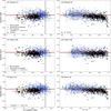Fig. 4

Log(S/O) as a function of 12+log(O/H) (left) and the ionisation degree, O²⁺/O (right), for H II regions or SFGs of the DESIRED-E sample having both S⁺ and S²⁺ abundances. Panels in the same row of the figure represent log(S/O) ratios calculated using the ICF(S) scheme by Amayo et al. (2021, top panels), Izotov et al. (2006, middle panels) and Dors et al. (2016, bottom panels). The dotted red line represents the mean value of the log(S/O) obtained using each ICF(S). The orange diamonds indicate the mean log(S/O) values considering bins in 12+log(O/H) or O²⁺/O. The black dashed lines and the grey bands show the solar 12+log(O/H) and log(S/O) ratios and their associated uncertainties, respectively, from Asplund et al. (2021).

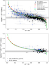Fig. 5

Log(Ar²⁺ /O²⁺) (top) and log((Ar²⁺+Ar³⁺)/O²⁺) (bottom) as a function of the ionisation degree, O²⁺/O, for DESIRED-E sample of H II regions (blue circles) and SFGs (black squares). The black dashed lines and the grey bands show the solar log(Ar/O) value and their associated uncertainty, respectively, from Asplund et al. (2021). The different curves represent the ICF(Ar) schemes used in this study: Amayo et al. (2021, shown as red dashed-dotted lines), Izotov et al. (2006, shown as dotted lines with colours corresponding to three metallicity ranges,) and Pérez-Montero et al. (2007, shown as green dashed lines).

5 The Ne/O, S/O, and Ar/O abundance ratios in the Local Universe

In this section, we discuss the results obtained in Sect. 4 in order to explore the behaviour of Ne/O, S/O, and Ar/O ratios with respect to metallicity in star-forming regions of the Local Universe. To do so, we first selected the ICF scheme that we consider works better for each element and focus the subsequent discussion on the results obtained with that chosen ICF. In the next step, we studied the behaviour of these ratios as a function of metallicity to analyse whether the nucleosynthetic origin of Ne, S, and Ar is, in fact, similar to that of O. We also tried to interpret possible departures. We also explored whether there are differences between the behaviour of these ratios as a function of the type of object: H II regions or SFGs. Finally, we established precise values of the Ne/O, S/O and Ar/O ratios representative of the ionised gas-phase of the ISM in the Local Universe.

5.1 Ne/O

Summarising the results analysed in Sect. 4.1 and Figs. 2 and 3, the ICF(Ne) by Izotov et al. (2006) shows a log(Ne/O) versus O²⁺/O ratio relation flatter than the other ICF(Ne) schemes as well as the lowest standard deviation and mean and median values of log(Ne/O) (−0.67 ± 0.12 and −0.66, respectively) more consistent with the solar ratio of −0.63 ± 0.06 (Asplund et al. 2021). For these reasons we have used the Ne abundances obtained with the ICF(Ne) by Izotov et al. (2006) for the discussion we present out in the present section. However, even if we made this choice, determining total Ne abundances using ICFs has serious limitations. As we point out in Sect. 4.1, an important fraction of the objects at values of O²⁺/O < 0.5, show very low log(Ne/O) values (see Fig. 3). In Fig. 2 it is evident that the position of those points cannot be correctly reproduced by any of the ICF(Ne) schemes considered. The strong increased scatter of the Ne²⁺/O²⁺ ratio at lower O²⁺/O is not something new, it was formerly reported by Kennicutt et al. (2003). Croxall et al. (2016), in their study of H II regions in the spiral galaxy NGC 5457 (M101), confirm a similar scatter, claiming for the existence of a large population of H II regions with significant offset to low values of log(Ne/O).

In Fig. 7, we show the distribution of log(Ne/O) as a function of 12+log(O/H) and O²⁺/O separately forH II regions and SFGs, for which Ne abundance has been derived using the ICF(Ne) by Izotov et al. (2006). The very different behaviour between both types of objects is striking. Since the distribution of the 557 data points classified as H II regions shows no significant indication of correlation (especially evident in the bottom left panel), the 671 SFGs represented in the top panels of Fig. 7 show a rather flat trend. The log(Ne/O) versus 12+log(O/H) relation for SFGs seems to follow a weak positive linear correlation with a rather small slope. In Fig. 7, we include a linear fit to the data points of SFGs considering their errors, represented by a continuous line. The mean and median values of log(Ne/O) and 12+log(O/H) for each type of object are given in Table 1. The parameters of the linear fit to the log(Ne/O) versus 12+log(O/H) and versus 12+log(Ne/H) distributions of the SFGs are given in Table 2. Although the sample Pearson correlation coefficient of the fit to log(Ne/O) versus 12+log(O/H) is rather low (r = 0.27), it seems to reproduce reasonably well the weak observational trend. In Table 2 we also include the p-value of the fits, that is used to evaluate the plausibility of the null hypothesis, which indicates the absence of correlation between the variables involved in the linear fit³. The fit shown in the upper left panel of Fig 7 indicates a small increase of log(Ne/O) of 0.08 dex for the interval of 12+log(O/H) between 7.0 and 8.5. Izotov et al. (2006), for a sample of 414 SFGs – most of them included in the DESIRED-E sample used in this paper – found also a slight increase of ~0.1 dex in the same interval of O abundances. Similar trends are found in the log(Ne/O) versus 12+log(O/H) distributions obtained by Amayo et al. (2021) and Miranda-Pérez & Hidalgo-Gámez (2023). Arellano-Córdova et al. (2024), who study 43 local SFGs of the COS Legacy Archive Spectroscopic SurveY (CLASSY), find a group of 5 SFGs (~10% of their sample) with 12+log(O/H) of the order or even above the solar value, showing log(Ne/O) ≥ −0.5, fact that they suggest may reflect some overproduction of Ne. Remarkably, our sample of SFGs do not present objects with such characteristics.

In Fig. 8, we represent log(Ne/O) versus 12+log(Ne/H) for the DESIRED-E sample of SFGs. The continuous red line shows a least-squares linear fit to the data considering their errors. The sample Pearson correlation coefficient of the fit is r = −0.64, a stronger linear correlation to that obtained for the log(Ne/O) versus 12+log(O/H) distribution shown in the top left panel of Fig. 7. The fit gives a slope only slightly higher than the one with respect to O/H and an increase of log(Ne/O) of 0.09 dex for the interval of 12+log(Ne/H) between 6.5 and 7.8. As we can see the fits to log(Ne/O) versus 12+log(O/H) and versus 12+log(Ne/H) of the SFGs are fairly similar and both clearly incompatible with the null hypothesis (see Table 2).

Nucleosynthesis models seem to agree in predicting a basically lockstep evolution of O and Ne (e.g. Iwamoto et al. 1999; Johnson 2019; Kobayashi et al. 2020). In Fig. 8, we also include a curve (green line) representing the evolution of Ne and O abundances of the ISM predicted by the chemical evolution model (CEM) of the Milky Way obtained by Medina-Amayo (2023). This CEM was developed for the solar neighborhood of the Galactic disc (7-9 kpc from the Galactic centre) within a two-infall gas formation scenario, similar to that of Spitoni et al. (2021). During the first 4 Gyr, the thick disc formed from a short accretion of primordial gas. Then, the thin disc began forming from a prolonged second accretion (the loop in the curve), which has continued to the present. The star formation rate and initial mass function (IMF) are based on the formulations of Kennicutt (1998) and Kroupa (2002), respectively. The model uses stellar yields for low-and intermediate-mass stars by Ventura’s group (e.g. Ventura et al. 2022, and references therein), for SNe Ia by Leung & Nomoto (2018), and for massive stars by Nomoto et al. (2013). An upper mass limit of the IMF at 37 M_⊙ was inferred to match the present-day O abundance of H II regions obtained from CELs at ~8 kpc (Méndez-Delgado et al. 2022a). In Fig. C.1, we show the cumulative fraction of ¹⁶O, ²⁰Ne, and ³⁶Ar, which are the most abundant stable isotopes of each element, that represent between 85 to 95% of the total amount of them, produced by different types of stars as a function of 12+log(O/H) predicted by the CEM. We distinguish the fractions produced by low- and intermediate-mass stars in the asymptotic giant branch phase (AGBs, cyan line) or type Ia supernovae (SNe Ia, dark red line) and massive stars in core collapse supernovae (CCSNe, magenta line). It is important to remember that the CEM used is built to reproduce the abundance patterns observed in the Milky Way. Objects in other galaxies with a different star-formation history may be located in somewhat different places in the abundance ratios diagrams. For example, the infall of unprocessed gas into a star-forming region in a galaxy may decrease the metal-licity, while keeping the abundance ratio of two alpha elements constant.

As we can see in Fig. 8, this CEM reproduces the log(Ne/O) of about −0.70 dex that show the low-metallicty SFGs represented in Fig. 8. However, the curve provides a rather slight increase of only +0.06 dex in the whole Ne/H range of the objects, an increase that seems insufficient to reproduce the trend we observe in our log(Ne/O) versus 12+log(Ne/H) distribution at higher metallicities. In principle, this behaviour may be interpreted as a slight metallicity-dependent Ne production but this is not predicted by nucleosynthesis models. In fact, Fig. C.1 shows that the SNe Ia and AGB contribution to the total amount of ¹⁶O and ²⁰Ne is very small and that the time evolution of Ne/O should produce a constant ratio. Izotov et al. (2006), assuming this lockstep evolution of O and Ne, interpret the increase of about 0.1 dex they find in their log(Ne/O) versus 12+log(O/H) relation (very similar to ours) as an effect of O depletion onto dust grains as a function of metallicity⁴. For the Orion Nebula – an example of a local H II region whose chemical composition is representative of the solar neighborhood – the fraction of dust trapping O is up to ~0.1 dex (e.g. Mesa-Delgado et al. 2009; Peimbert & Peimbert 2010). In a recent paper, Méndez-Delgado et al. (2024) estimated that at the metallicities of the Magellanic Clouds (Large Magellanic Cloud, LMC: 12+log(O/H) = 8.36, Small Magellanic Cloud, SMC: 8.03; Domínguez-Guzmán et al. 2022); we note that such O depletion should account for up to 0.07 dex and 0.03 dex for LMC and SMC, respectively, becoming negligible at 12+log(O/H) < 8.0. This seems to be roughly consistent with the hypothesis of the dust depletion to explain the observed log(Ne/O) versus 12+log(O/H) or versus 12+log(Ne/H) correlations, but also with the offset of about ~0.10 dex between the log(Ne/O) given by the CEM predictions and observations at high metallicities. In principle, the dust depletion hypothesis could be verified if we found a similar behaviour with other noble gases such as Ar (also proposed by Amayo et al. 2021). However, as we discuss in Sect. 5.3 and can be seen in Fig. C.1, the nucle-osynthetic origin of Ar does not seem to be entirely similar to that of O or Ne, so the behaviour of the Ar/O ratio may be modulated by other phenomena apart from a different degree of dust depletion relative to O.

Another possibility to explain the slight increase of log(Ne/O) as a function of metallicity is that it is an artifact produced by the ICF(Ne) itself. As we can see, the mean log(Ne/O) values corresponding to the 0.1 dex wide bins in O²⁺/O shown in the upper right panel of Fig. 7 trace a rather slight tendency to decrease as O²⁺/O increases. This might ultimate contribute in some way to the increase of log(Ne/O) with metallicity we have observed. In fact the maximum amplitude of the variation of log(Ne/O) between the O²⁺/O bins represented in Fig. 7 is of about 0.06 dex.

As we pointed out above, in Fig. 7, the behaviour of H II regions is very different to that shown by SFGs. In the log(Ne/O) versus 12+log(O/H) diagram, the observational points classified as H II regions are distributed in a quite defined range of metal-licity but with a much larger dispersion of log(Ne/O). We can distinguish that although most of the objects are concentrated at log(Ne/O) values close to the solar one, there seems to be a secondary concentration at 12+log(O/H) ~ 8.4 and log(Ne/O) between -1.0 and -0.7. In fact, in Table 1 the mean log(Ne/O) of the H II regions is 0.07–0.08 dex lower than the mean of the SFGs or the solar value. Croxall et al. (2016) and Berg et al. (2020) find a similar log(Ne/O) versus 12+log(O/H) distribution, although this was expected given that the observational data on which those studies are based are included in the DESIRED-E sample. The log(Ne/O) versus O²⁺/O diagram of the bottom row of Fig. 7 shows that the dispersion towards lower values of log(Ne/O) is clearly a function of O²⁺/O, indicating that the ICF(Ne) is not able to correct appropriately for the presence of Ne⁺ in H II regions data points at O²⁺/O ≤ 0.75, which are the vast majority of the objects of this type in the DESIRED-E sample. Kennicutt et al. (2003) suggested that this behaviour is due to the high sensitivity of Ne ionisation models to the input stellar atmosphere fluxes, which in turn are very much dependent on the treatment of opacity and stellar winds. Considering the difficulties of obtaining consistent Ne/O values from Galactic and extragalactic H II regions, we have chosen not to take them into account for the study of the behaviour of this ratio as a function of metallicity and in the data shown in Table 2.

In Fig. 9, we present the log(Ne/O) versus 12+log(O/H) distribution of H II regions and SFGs of the DESIRED-E sample, the curve defined by the CEM of Medina-Amayo (2023) and abundances of O and B-type Galactic stars determined from quantitative spectroscopy by Nieva & Przybilla (2012), Weßmayer et al. (2022) and Aschenbrenner et al. (2023). The atmospheres of O and B-type stars represent the present-day chemical composition of the ISM and, in principle, should provide abundance values similar to the ionised gas associated with star-forming regions. In Fig. 9, we can see that the stellar O abundances are close to solar or oversolar (as expected because most of the stars are located in the solar neighborhood), but quite separated from the locus of the bulk of the H II regions. A systematic difference between nebular and stellar abundances of objects located in the same star-forming regions is a well-known fact. Studies comparing the O abundances of Galactic H II regions with that of their associated O and B-type stars (e.g. Simón-Díaz et al. 2006; Simón-Díaz & Stasińska 2011; García-Rojas et al. 2014) find stellar abundances ~0.2 dex higher than nebular ones when they are calculated using CELs. However, such difference disappears when using faint recombination lines instead of CELs for deriving the nebular O abundance, this offset is the so-called abundance discrepancy problem. It may be related to the presence of temperature fluctuations inside the H II regions (Peimbert 1967; García-Rojas et al. 2007; Méndez-Delgado et al. 2023b). On the other hand, Fig. 9 indicates that the O and B-type stars also show a quite high dispersion in their log(Ne/O) ratio. The mean and standard deviation of log(Ne/O) of the stars included in the figure is −0.56 ± 0.17, a fairly supersolar value. Although temperature fluctuations can alter the abundances calculated with CELs, the abundance ratios (as Ne/O, S/O, or Ar/O) obtained with this type of lines remain practically unchanged, so the observed log(Ne/O) offset between stellar and nebular objects is not expected to be related to this phenomenon (e.g. Esteban et al. 2020; Méndez-Delgado et al. 2024).

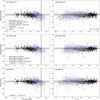Fig. 6

Log(Ar/O) as a function of 12+log(O/H) (left) and the ionisation degree, O²⁺/O (right), for the DESIRED-E H II regions (blue circles) or SFGs (black squares) having only Ar²⁺ (empty symbols) or Ar²⁺ and Ar³⁺ abundances (full symbols). Panels in the same row of the figure represent log(Ar/O) calculated using the ICF(Ar) scheme of Amayo et al. (2021, top panels), Izotov et al. (2006, middle panels) and Pérez-Montero et al. (2007, bottom panels). The dotted red line represents the mean value of log(Ar/O) obtained using each ICF(Ar). The orange diamonds indicate the mean log(Ar/O) values defined by all the points represented considering bins in 12+log(O/H) or O²⁺/O. The black dashed lines and the grey bands show the solar 12+log(O/H) and log(Ar/O) and their associated uncertainties, respectively, from Asplund et al. (2021).

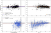Fig. 7

log(Ne/O) as a function of 12+log(O/H) (left) and the ionisation degree, O²⁺/O (right), for the DESIRED-E sample. The values of log(Ne/O) are calculated using the ICF(Ne) scheme by Izotov et al. (2006). The top panels show the points corresponding to SFGs (black squares) and the bottom panels the corresponding to H II regions (blue circles). Orange diamonds in the top right panel indicate the mean log(Ne/O) values considering bins in O²⁺/O. The blue continuous line included in the top left panel represents a linear fit to the data of SFGs. The dotted red line represents the mean value of the log(Ne/O) obtained for each kind of object. The black dashed lines and the grey bands show the solar 12+log(O/H) and log(Ne/O) and their associated uncertainties, respectively, from Asplund et al. (2021).

Table 1

Mean and median abundance ratios per element X and type of object.

Table 2

Linear fits log(X/O) = m × [12+log(Y/H)] + n per element X and type of object.

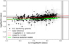Fig. 8

log(Ne/O) as a function of 12+log(Ne/H) for SFGs of the DESIRED-E sample, which Ne/O ratios have been calculated using the ICF(Ne) scheme by Izotov et al. (2006). The red continuous line represents a linear fit to the data. The green continuous line shows the time evolution of Ne and O abundances of the ISM predicted by the CEM of the Milky Way of Medina-Amayo (2023). The dotted red line represents the mean value of log(Ne/O). The black dashed lines and the grey bands show the solar 12+log(Ne/H) and log(Ne/O) and their associated uncertainties, respectively, from Asplund et al. (2021).

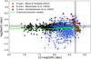Fig. 9

log(Ne/O) as a function of 12+log(O/H). Black squares and blue circles represent SFGs and H II regions of the DESIRED-E sample, which Ne/O ratios have been calculated using the ICF(Ne) scheme by Izotov et al. (2006). The green continuous line shows the time evolution of Ne and O abundances of the ISM predicted by the CEM of the Milky Way of Medina-Amayo (2023). Yellow and orange stars represent the abundances obtained from quantitative spectroscopic analysis of Galactic B stars by Nieva & Przybilla (2012) and Weßmayer et al. (2022), respectively. Magenta stars represent the abundances of Galactic O stars determined by Aschenbrenner et al. (2023). The black dashed lines and the grey bands show the solar 12+log(O/H) and log(Ne/O) and their associated uncertainties, respectively, from Asplund et al. (2021).

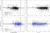Fig. 10

log(S/O) as a function of 12+log(O/H) (left) and the ionisation degree, O²⁺/O (right), for the DESIRED-E sample. The values of log(S/O) are calculated using the ICF(S) scheme by Izotov et al. (2006). The top panels show the points corresponding to SFGs (black squares) and the bottom panels the corresponding to H II regions (blue circles). The dotted red line represents the mean value of the log(S/O) obtained for each kind of object. The blue continuous lines represent linear fits to the data represented in each panel of the left column. The black dashed lines and the grey bands show the solar 12+log(O/H) and log(S/O) and their associated uncertainties, respectively, from Asplund et al. (2021).

5.2 S/O

As in the case of the Ne/O ratio discussed in Sect. 5.1, the ICF(S) by Izotov et al. (2006) is the one that provides a more featureless – flatter – distribution between log(S/O) versus 12+log(O/H) and versus O²⁺/O (Fig. 3), a tighter fit to the (S⁺+S²⁺)/O versus O²⁺/O distribution in the range of ionisation degrees in common with the others ICFs (Fig. 2) and a mean log(S/O) closer to the solar value of −1.57 ± 0.05 (Asplund et al. 2021). We adopted the results obtained using this ICF(S) for the discussion developed in this section. The only drawback of the ICF(S) scheme by Izotov et al. (2006) is that its application is limited to objects with O²⁺/O ≥ 0.2. In the case of the DESIRED-E sample this has a very limited impact. While no SFGs have to be removed applying this limit, the fraction of H II regions that are finally excluded is only 13.3%. Considering the rough relation between ionisation degree and metallicity shown in Fig. B.1, this implies that the removed points correspond mostly to high metallicity objects but (as we can see in the panels of the left column of Fig. 4) that area is not significantly depopulated when we compare the results using the different ICF(S) schemes.

The results of most studies indicate that the S/O ratio remains basically constant with respect to O/H (e.g. Garnett et al. 1997; Kennicutt et al. 2003; Izotov et al. 2006; Guseva et al. 2011; Croxall et al. 2016; Berg et al. 2020; Arellano-Córdova et al. 2020, 2024). Although there are others who claim that S/O decreases as O/H increases (eg. Vilchez et al. 1988; Dors et al. 2016; Díaz & Zamora 2022; Pérez-Díaz et al. 2024; Brazzini et al. 2024). In Fig. 10, we show the distribution of log(S/O) as a function of 12+log(O/H) and O²⁺/O separately for SFGs and H II regions. The S/O ratios have been calculated using the ICF(S) scheme by Izotov et al. (2006). Unlike log(Ne/O) (see Fig. 7), the behaviour of log(S/O) is qualitatively very similar in both types of objects. However, the mean value of log(S/O) and its standard deviation are somewhat different; in the case of SFGs we obtain − 1.64 ± 0.13 (median −1.65) and −1.54 ± 0.19 (median −1.58) for HII regions (see Table 1), being closer to solar (−1.57 ± 0.05; Asplund et al. 2021) in this last type of objects. In Fig. 10 we include the linear fits to log(S/O) versus 12+log(O/H) for SFGs and H II regions (their parameters are listed in Table 2), finding that the distribution of the data points is rather flat in both cases, specially for the objects classified as H II regions, fact that is consistent with a constant and solar log(S/O). This is also confirmed by the large p-value of the fit for H II regions or the combination of H II regions plus SFGs, that are consistent with the null hypothesis.

In Fig. 11, we present the log(S/O) versus 12+log(O/H) (top) and versus 12+log(S/H) (bottom) distributions of SFGs+H II regions of the DESIRED-E sample. In the top panel we also include abundances of Galactic B-type stars determined by Weßmayer et al. (2022) and classical Cepheids observed and analysed by da Silva et al. (2023). Classical or Population I Cepheids are variable stars with masses in the interval of 4 and 20 M_⊙ (Turner 1996) and ages ≲300 Myr (Bono et al. 2005); thus, (as B-type stars) their atmospheric abundances should also be representative of the presentday chemical composition of the ISM. As in the case of Ne/O versus O/H diagram shown in Fig. 9, the O/H values in Galactic stars are close to solar or oversolar and are distributed in a separated locus from the bulk of the nebular objects, even the Galactic ones. This fact has already been discussed in Sect. 5.1. On the other hand, the mean log(S/O) values of the B-type stars represented in Fig. 11 is −1.68 ± 0.08 and that of the classical Cepheids −1.64 ± 0.15, both values below the solar log(S/O) of −1.57 ± 0.05. In Fig. 11, we can notice that the S/O ratio of classical Cepheids seem to show a clear decrease as O/H increases, a fact already noticed by da Silva et al. (2023).

The behaviour of the data points of the DESIRED-E sample shown in Figs. 10 and 11 contrasts with the results obtained by some previous studies (Dors et al. 2016; Díaz & Zamora 2022; Brazzini et al. 2024). In particular, Díaz & Zamora (2022) find that S/O versus O/H and versus S/H relations are quite different for SFGs and H II regions. Díaz & Zamora (2022) report that SFGs tend to show a S/O ratio lower than solar and that it increases as the S/H increases, but remains constant with O/H, results that are in agreement with ours. However, they find that their H II regions show S/O ratios larger than solar and a clear tendency for lower S/O ratios as O or S abundances increase, a behaviour different to what we observe. In our case, for H II regions, since log(S/O) remains basically constant with 12+log(O/H), it shows a clear increase as 12+log(S/H) increases (see Table 2). In trying to understand the origin of the discrepancy with the results by Díaz & Zamora (2022), we realized that the O/H ratios of at least some of the H II regions of the sample of Díaz & Zamora (2022) were lower than those determined by us for the same objects and clearly incorrect⁵, producing spurious higher S/O ratios. It is beyond the scope of this paper to investigate the origin and quantify the errors in the abundances calculated in Díaz & Zamora (2022), but we consider that part of their conclusions, at least those based on the chemical behaviour of the H II regions – apparently no the SFGs – should not be taken into account until the authors provide the correct abundances. Unfortunately, the results obtained by Díaz & Zamora (2022) has led to studies exploring their origin and implications as, for example, Goswami et al. (2024), who proposed that such high S/O values might be explained by the contribution of the ejecta of Pair Instability Supernovae (PISN) produced by very massive stars (≥130 M_⊙) in combination of a bi-modal top-heavy IMF and an initial strong burst of star formation. Ultimately, it is not necessary to invoke such exotic scenarios to explain the correct abundance patterns.

In Fig. 11, we include the curves defined by the CEM of Kobayashi et al. (2020)⁶ and a least-squares fit to all the data (SFGs+H II regions) considering their errors (their parameters are listed in Table 2). The slopes of the linear fits are quite different and significantly higher for the log(S/O) versus 12+log(S/H) distribution. The sample Pearson correlation coefficient of the log(S/O) versus 12+log(O/H) fit is almost 0 and its p-value indicates that the distribution is indistinguishable of the null hypothesis. Therefore, we can conclude that the log(S/O) versus 12+log(O/H) distribution of all the data is basically constant. This is not entirely consistent with the behaviour predicted by the CEM, where we would expect an increase of log(S/O) of the order of +0.30 dex in the range of metallicities covered by the objects. On the other hand, the fit to log(S/O) versus 12+log(S/H) for SFGs+H II regions shows a clearer trend with a more positive slope, a moderate sample Pearson correlation coefficient and extremely low p-values (see Fig. 11 and Table 2). As we can see in Table 2, the same higher and positive slope of the fit when considering 12+log(S/H) instead of 12+log(O/H) remains when separating H II regions and SFGs. Díaz & Zamora (2022) also find a greater dependence of the S/O ratio on S/H than on O/H in the case of SFGs, objects that apparently have correct O abundances in their paper. Figure 11 indicates that comparison with the CEM seems to be more consistent in this case. The model curve fits fairly well to the distribution of the different bins. In particular, the bins corresponding to 12+log(S/H) . 6.0 show a flat trend, consistent with the behaviour and the average log(S/O) given by the model. At 12+log(S/H) ≥ 6.0, a slight but continuous increase in S/O occurs, so the lockstep evolution of both elements is not longer achieved. Nucleosynthesis models for SNe Ia predict that these objects may produce a significant fraction of the S and Ar content in the solar neighbourhood (e.g. Iwamoto et al. 1999; Johnson 2019; Kobayashi et al. 2020). The Chandrasekhar-mass explosion models for SNe Ia by Kobayashi et al. (2020) predict that about 29% of the total solar S originates from this process, although this fraction might be even higher if the contribution of sub-Chandrasekhar-mass SNe Ia is increased in their models.

Finally, although the linear fit to log(S/O) versus 12+log(O/H) presents a small (but rather uncertain) positive slope that could be consistent with the hypothesis on O depletion put forward in Sect. 5.1 to explain the behaviour of the Ne/O ratio, it cannot be verified in the case of S/O. Firstly because (as discussed in the previous paragraph) the production of S by SNe Ia also produces an increase in S/O with O/H. Secondly, the fraction of S depleted onto dust grains in the ISM is a controversial issue because the spectral features used to study it are often highly saturated (e.g Jenkins 2009). In fact, it is often referred to as the ‘missing sulfur problem’ and has raised a variety of questions over the past two decades. (e.g. Keller et al. 2002; Slavicinska et al. 2025).

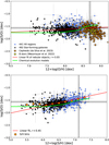Fig. 11

log(S/O) as a function of 12+log(O/H) (top) and as a function of 12+log(S/H) (bottom). Black squares and blue circles represent SFGs and H II regions of the DESIRED-E sample, which S/O ratios have been calculated using the ICF(S) scheme by Izotov et al. (2006). The green continuous line shows the time evolution of S and O abundances of the ISM predicted by the CEM of the Milky Way of Kobayashi et al. (2020). Yellow stars represent the abundances obtained from quantitative spectroscopic analysis of Galactic B stars by Weßmayer et al. (2022). Orange stars represent the abundances of Galactic classical Cepheids determined by da Silva et al. (2023). Orange diamonds indicate the mean log(S/O) values considering bins in 12+log(S/H). The red continuous lines represent linear fits to the data represented in each panel. The black dashed lines and the grey bands show the solar 12+log(O/H), 12+log(S/H) and log(S/O) and their associated uncertainties, respectively, from Asplund et al. (2021).

5.3 Ar/O

In Sect. 4.3, we conclude that the different ICF(Ar) schemes considered show a very similar behaviour of the Ar/O ratio with respect to the O abundance and degree of ionisation, so the analysis of the Ar/O ratio seems to be independent of the final selection of the ICF(Ar) scheme. In fact, Fig. A.1 indicates that the differences in the Ar/H computed using any pair of ICF(Ar) schemes are lower than 0.04 dex when O²⁺/O < 0.95 but not much larger than 0.10 for higher ionised objects. Thus, we finally decided to use the ICF(Ar) by Izotov et al. (2006) to maintain consistency with the results obtained with the rest of the alpha elements and to remove the objects with lower ionisation degree (O²⁺/O < 0.2), where the contribution of unseen Ar⁺ is larger. This allows the elimination of objects where the ICF(Ar) value is higher and minimizes the systematic uncertainty introduced by the use of an ICF.

Most works have reported an almost constant Ar/O versus O/H distribution (e.g. Izotov et al. 2006; Hägele et al. 2008; Croxall et al. 2016; Miranda-Pérez & Hidalgo-Gámez 2023). However, several works have established some correlation (e.g. Pérez-Montero et al. 2007; Arnaboldi et al. 2022; Arellano-Córdova et al. 2024). In Fig. 12, we show the distribution of log(Ar/O) as a function of 12+log(O/H) and O²⁺/O separately for H II regions and SFGs. In all cases we have used the ICF(Ar) scheme by Izotov et al. (2006). As in previous figures, we distinguish between those points whose Ar/H ratios have been derived solely using [Ar III] lines from those that have been determined using both [Ar III] and [Ar IV] ones⁷. As can be noted in Fig. 12 and the fits parameters given in Table 2, the behaviour of log(Ar/O) versus 12+log(O/H) and O²⁺/O is very similar for H II regions and SFGs. The log(Ar/O) versus 12+log(O/H) distribution of both kinds of objects follow rather clear linear relationships with negative slopes. Their sample Pearson correlation coefficients are moderate but the corresponding p-values very small (see Table 2). The trend of decreasing Ar/O ratios as O/H increases is quite unexpected but it has been also observed in several previous works (Pérez-Montero et al. 2007; Kojima et al. 2021; Arellano-Córdova et al. 2024). In the right panels of Fig. 12, we include also the mean log(Ar/O) in different O²⁺/O bins of 0.1 units wide. In the case of H II regions, the trend is basically constant with a maximum difference of log(Ar/O) of ~0.05 dex. For SFGs the trend shows some undulation and log(Ar/O) increases slightly as O²⁺/O increases, but the maximum difference is only 0.11 dex. The results shown in these two panels of Fig. 12 indicate that any trend we observe in the distribution of log(Ar/O) as a function of metallicity is basically independent of the ICF(Ar). The mean value of log(Ar/O) is −2.37 ± 0.12 in the case of SFGs and −2.30 ± 0.20 for HII regions, both consistent with the solar value of −2.31 ± 0.11 (Asplund et al. 2021).

In Fig. 13, we present the log(Ar/O) versus 12+log(O/H) (top) and versus 12+log(Ar/H) (bottom) distributions of SFGs+H II regions of the DESIRED-E sample. We have represented the data points with the same symbol regardless of whether [Ar III] or [Ar III]+[Ar IV] lines were used to determine the Ar abundance. As in some previous figures, in Fig. 13 we also include a least-squares fit to the data represented in each panel. The two distributions show weak correlations with slopes of different signs. Although the sample Pearson correlation coefficients of the linear fits to log(Ar/O) versus 12+log(O/H) and versus 12+log(Ar/H) distributions are r = −0.28 and 0.17, respectively, their very low p-values indicate that both correlations can be considered real. As in the case of the fits separated by type of object, the fit to log(Ar/O) versus 12+log(O/H) for SFGs+H II regions indicates a decrease of log(Ar/O) of 0.24 dex in the whole interval of 12+log(O/H) represented in the top panel of Fig. 13. This behaviour is contradictory to what is expected from current nucleosynthesis and chemical evolution models. In fact, the curve predicted by the CEM of Medina-Amayo (2023) included in Fig. 13 would imply an increase of the Ar/O ratio with metallicity, in clear disagreement with the general behaviour shown by our data. This puzzling result deserves further study.

In the case of the log(Ar/O) versus 12+log(Ar/H) distribution shown in Fig. 13, we find a weak linear correlation with a small positive slope and a total increase of log(Ar/O) of 0.12 dex in the entire Ar/H range. Although the predictions of the CEM are now qualitatively consistent with the data, they are not quantitatively consistent. The CEM predicts an increase of 0.54 dex over the range of Ar abundances represented in Fig. 13, considerably higher than observed. On the other hand, unlike what happens in the cases of Ne and S, the CEM also does not reproduce the mean log(Ar/O) at low metallicities. The predicted value is about 0.10 dex lower than observed, but this cannot possibly be due to depletion of O onto dust grains because it is expected to be negligible at such low metallicities.

Regarding the log(Ar/O) versus 12+log(Ar/H) distribution obtained by other authors, the results are disparate. Arellano-Córdova et al. (2024) and Miranda-Pérez & Hidalgo-Gámez (2023) obtain a quite flat distribution in the log(Ar/O) versus 12+log(Ar/H) relation at intermediate values of 12+log(Ar/H) but opposite trends in low and high values of the Ar abundance. In particular, Miranda-Pérez & Hidalgo-Gámez (2023) find a rather strong increase of log(Ar/O) for objects with 12+log(Ar/H) > 6.0, reaching values larger than in any SFG of our DESIRED-E sample. On the other hand, Arnaboldi et al. (2022) studied the behaviour of the Ar/O versus Ar/H relation for a sample of planetary nebulae in the M31 galaxy. They find an increase of the Ar/O ratio as the Ar/H increases but in a rather narrow interval of 12+log(Ar/H), between 6.0 and 6.5 approximately, in agreement with the predictions of the chemical evolution models of the Milky Way thick disc and solar neighbourhood of Kobayashi et al. (2020). Arnaboldi et al. (2022) interpret the increase in the log(Ar/O) versus 12+log(Ar/H) plane they observe as due to the contribution of SNe Ia. In fact, the models by Kobayashi et al. (2020) predict that about 34% of the total solar Ar is produced by SNe Ia. Figure C.1 also indicates that in the CEM of Medina-Amayo (2023) the increase of Ar/O with metallicity is produced basically by SNe Ia. We do not see an Ar/O increase as large as that reported by Arnaboldi et al. (2022), and our results are broadly consistent with a constant log(Ar/O) distribution in most of the 12+log(Ar/H) range. However, the bins represented in the bottom panel of our Fig. 13 suggest a slight increase (of only ~0.1 dex) for values of 12+log(Ar/H) ≥ 6.0, which (as we demonstrate in Fig. 12) does not appear to be an artifact of the ICF(Ar). In principle, our linear fit to the log(Ar/O) versus 12+log(Ar/H) distribution could be interpreted as an indication of a certain contribution by SNe Ia, although in a more limited proportion than that proposed by Arnaboldi et al. (2022).

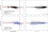Fig. 12

log(Ar/O) as a function of 12+log(O/H) (left) and the ionisation degree, O²⁺/O (right), for the DESIRED-E sample. The values of log(Ar/O) are calculated using the ICF(Ar) scheme by Izotov et al. (2006). Empty symbols indicate Ar abundances determined solely from [Ar III] lines and full symbols those determined using [Ar III] and [Ar IV] lines. The top panels show the points corresponding to SFGs (black squares) and the bottom panels the corresponding to H II regions (blue circles). Orange diamonds indicate the mean log(Ar/O) values considering bins in O²⁺/O. The red continuous lines represent linear fits to the data represented in each panel. The dotted red line represents the mean value of the log(Ar/O) obtained for each kind of object. The black dashed lines and the grey bands show the solar 12+log(O/H) and log(Ar/O) and their associated uncertainties, respectively, from Asplund et al. (2021).

6 Conclusions

In this paper, we analyse the behaviour of Ne/O, S/O and Ar/O abundance ratios with respect to metallicity in star-forming regions of the Local Universe, using the spectroscopical data compiled in the DEep Spectra of Ionised REgions Database (DESIRED) Extended project (DESIRED-E) (Méndez-Delgado et al. 2023a, 2024). DESIRED-E comprises almost two thousand high-quality spectra of H II regions and star-forming galaxies (SFGs) from the literature having direct determinations of T_e . For this study, we recalculated the physical conditions and ionic and total abundances of O, Ne, S, and Ar in a homogeneous manner for all the objects. We have a total number of 1386 spectra for which we can determine the total abundance of one, two, or three of the alpha elements considered: Ne, S, and Ar. Of that number, 50% are classified as H II regions and 50% as SFGs.

We compared the Ne/O, S/O, and Ar/O abundance ratios obtained using three different ICF schemes for each element. Two of them: Amayo et al. (2021) and Izotov et al. (2006) are common to Ne, S and Ar, and the third ICF scheme is different for each element: Dors et al. (2013) for Ne, Dors et al. (2016) for S and Pérez-Montero et al. (2007) for Ar. After a careful analysis, we conclude that the ICF scheme proposed by Izotov et al. (2006) seems to better reproduce the behaviour of the three abundance ratios. It produces a less dependent (flatter) distribution of Ne/O, S/O, and Ar/O with respect to O²⁺/O and a smaller dispersion in the mean value of each ratio, which is consistent with the solar value.

We derived Ne/O ratios for 1228 DESIRED-E spectra, of those 557 correspond to H II regions and 671 to SFGs. The log(Ne/O) versus 12+log(O/H) distribution of H II regions displays a large dispersion and no evidence of correlation. Our analysis indicates that the position of those objects cannot be correctly reproduced by any of the ICF(Ne) schemes considered. Therefore, we do not recommend the use of these objects for the study of the cosmic evolution of Ne. On the other hand, the SFGs show much lower dispersion in their Ne/O ratios and rather similar log(Ne/O) versus 12+log(O/H) and log(Ne/O) versus 12+log(Ne/H) linear relations with positive, but small slopes. These correlations may be due to several factors or a combination of them. Firstly, the effect of a metallicity-dependent O depletion fraction that increases throughout the metallicity range covered by the objects. Secondly, an effect of the ICF(Ne), which does not completely cancel out the Ne/O dependence on O²⁺/O. A third possibility would be a certain unknown mechanism producing Ne, but chemical evolution models do not predict such scenario (at least not to a significant extent).

To achieve more confident determinations, we only considered objects for which their S/H ratio can be determined from the sum of S⁺ and S²⁺ abundances. Considering this, the log(S/O) versus 12+log(O/H) relationship that we found separately for 441 and 492 spectra of HII regions and SFG of our sample is compatible with a constant value (especially for H II regions) and when we combine all the sample objects (H II regions + SFGs); this is in contrast to what was found in some previous works (Dors et al. 2016; Díaz & Zamora 2022; Brazzini et al. 2024). In this regard, we have found that at least part of the results of Díaz & Zamora (2022) are incorrect, so some of their conclusions should be revised. We found a rather tight and positive linear fit for all the objects when we use the log(S/O) versus 12+log(S/H) distribution. It is remarkable that the predictions of the CEM by Kobayashi et al. (2020) fit that distribution fairly well across the whole S/H range. We propose that the positive slope the log(S/O) versus 12+log(S/H) relation and its change of slope at 12+log(S/H) ~ 6.0 can be interpreted as an observational evidence of contribution of S produced by SNe Ia.

The behaviour of log(Ar/O) versus 12+log(O/H) and O²⁺/O is very similar for our sample of 447 spectra of H II regions and 506 of SFGs and seems to be independent of the O²⁺/O ratio and the type of ICF(Ar) used, whether it is based on only the [Ar III] lines or on the sum of [Ar III] and [Ar IV]. The fit to log(Ar/O) versus 12+log(O/H) indicates a slight decrease of log(Ar/O) as 12+log(O/H) increases, which is an unexpected behaviour. However, the log(Ar/O) versus 12+log(Ar/H) relation shows a inverse trend, with a small positive slope that might be interpreted as an indication of a small contribution from SNe Ia, smaller than predicted by recent nucleosynthesis models.

The mean value of log(Ne/O) for our sample of SFGs is −0.64 ± 0.07, almost coincident with the solar value of −0.63 ± 0.06 recommended by Asplund et al. (2021). Due to the low reliability of the ICF(Ne) for estimating the total Ne abundance of H II regions, we cannot define a precise mean value of log(Ne/O) for these objects. In the case of log(S/O) the mean value for SFGs and H II regions is −1.63 ± 0.13 and −1.54 ± 0.19, respectively, the latter value being more consistent with the solar one of −1.57 ± 0.05. For log(Ar/O) our results are −2.37 ± 0.12 and −2.30 ± 0.20 for SFGs and H II regions, respectively; again, this is more consistent with the solar value of −2.31 ± 0.11 in the case of H II regions. Considering that the mean 12+log(O/H) is 8.40 for our sample of H II regions and 8.05 for SFGs, the fact that both the mean log(S/O) and log(Ar/O) are larger in H II regions than in SFGs (about 0.11 and 0.07 dex, respectively) indicates that both ratios increase with metallicity. This result is consistent with a scenario that accounts for some additional contribution from S and Ar due to the presence of SNe Ia.

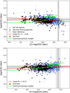Fig. 13

log(Ar/O) as a function of 12+log(O/H) (top) and as a function of 12+log(Ar/H) (bottom). Black squares and blue circles represent starforming galaxies and H II regions of the DESIRED-E sample, which Ar/O ratios have been calculated using the ICF(Ar) scheme by Izotov et al. (2006). The orange diamonds indicate the mean log(Ar/O) values considering bins in 12+log(O/H) or 12+log(Ar/H). The red continuous lines represent linear fits to the data represented in each panel. The green continuous line shows the time evolution of Ar and O abundances of the ISM predicted by the CEM of the Milky Way of Medina-Amayo (2023). The black dashed lines and the grey bands show the solar 12+log(O/H), 12+log(Ar/H) and log(Ar/O) and their associated uncertainties, respectively, from Asplund et al. (2021).

Data availability

The complete tables of atomic data, references, physical conditions and abundances for all the objects in our sample can be found at: https://zenodo.org/records/15005362.

Acknowledgements

We thank the anonymous referee whose comments helped us improve the quality of the paper. CE, JGR, ERR and MOG acknowledge financial support from the Agencia Estatal de Investigación of the Ministerio de Cien-cia, Innovación y Universidades under grant “The internal structure of ionised nebulae and its effects in the determination of the chemical composition of the interstellar medium and the Universe” with reference PID2023-151648NB-I00 (DOI:10.13039/5011000110339). JGR also acknowledges financial support from the AEI-MCINN, under Severo Ochoa Centres of Excellence Programme 2020– 2023 (CEX2019-000920-S), and from grant “Planetary nebulae as the key to understanding binary stellar evolution” with reference PID-2022136653NA-I00 (DOI:10.13039/501100011033) funded by the Ministerio de Ciencia, Innovación y Universidades (MCIU/AEI) and by ERDF “A way of making Europe” of the European Union. JEMD acknowledges support from project UNAM DGAPA-PAPIIT IG 101025, Mexico. LC acknowledges support from the Fundación Occident and the Instituto de Astrofísica de Canarias under the Visiting Researcher Programme 2022–2024 agreed between both institutions.

Appendix A Comparison between ICF schemes

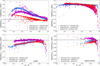Fig. A.1

Difference of the logarithmic Ne (top left), S (top right) and Ar (bottom panels) abundances calculated from the spectra of the DESIRED-E sample using various ICF schemes. In the bottom left panel we use ICF(Ar) using only [Ar III] lines and in the bottom right panel [Ar III] and [Ar IV] lines. The different symbols represent the pairs of ICF used in each case. The horizontal black line indicates equal abundance. Amayo+21: Amayo et al. (2021); Izotov+06: Izotov et al. (2006); Dors+13: Dors et al. (2013); Dors+16: Dors et al. (2016); and PM+07: Pérez-Montero et al. (2007).

Appendix B Relation between the oxygen abundance and ionisation degree

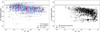Fig. B.1

12+log(O/H) as a function of the ionisation degree, O²⁺/O, for DESIRED-E sample of Galactic and extragalactic H II regions (blue circles, left panel) and star-forming galaxies (black squares, right panel). The red diamonds and lines indicate the mean 12+log(O/H) values and its standard deviation, considering bins of 0.2 in O²⁺/O.

Appendix C Relative contribution to O, Ne, and Ar enrichment by three different types of stars considered in the chemical evolution model

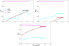Fig. C.1

Cumulative fraction of the contribution of different types of stars to ¹⁶O, ²⁰Ne, and ³⁶Ar (the most abundant stable isotopes of each element) enrichment as a function of 12+log(O/H) predicted by the chemical evolution model of Medina-Amayo (2023). Cyan line: asymptotic giant branch stars (AGBs); dark red line: type Ia supernovae (SNe Ia); magenta line: core collapse supernovae (CCSNe).

Appendix D Tables of atomic data, references, physical conditions, and abundances

The complete reference tables associated with Appendix D can be found at: https://zenodo.org/records/15005362.

The references for the atomic data used per ion are: O⁺ : Froese Fischer & Tachiev (2004), Kisielius et al. (2009); O²⁺ : Storey & Zeippen (2000), Storey et al. (2014), Wiese et al. (1996); Ne²⁺: McLaughlin et al. (2011); S⁺: Irimia & Froese Fischer (2005), Tayal & Zatsarinny (2010); S²⁺ : Froese Fischer et al. (2006), Grieve et al. (2014); Cl²⁺ : Butler & Zeippen (1989), Fritzsche et al. (1999); Ar²⁺: Galavis et al. (1995), Kaufman & Sugar (1986), Mendoza (1983); Ar³⁺: Mendoza & Zeippen (1982), Ramsbottom & Bell (1997); Fe²⁺: Deb & Hibbert (2009), Mendoza et al. (2023), Zhang (1996).

The references for the spectroscopic data are: Arellano-Córdova et al. (2016, 2021); Aver et al. (2022); Berg et al. (2013, 2015, 2016, 2020, 2021); Bresolin (2007, 2011a,b); Bresolin et al. (2004, 2005, 2007, 2009b,a, 2010); Castellanos et al. (2002); Crockett et al. (2006); Croxall et al. (2015, 2016); Delgado-Inglada et al. (2016); Díaz et al. (2000); Domínguez-Guzmán et al. (2022); Edmunds & Pagel (1984); Egorova et al. (2021); Esteban & García-Rojas (2018); Esteban et al. (2004, 2009, 2013, 2014, 2017, 2020); Fernández et al. (2018, 2022); Fernández-Martín et al. (2017); García-Rojas et al. (2004, 2005, 2006, 2007); Garnett & Kennicutt (1994); Garnett et al. (1997); Goddard et al. (2011); Gómez-González et al. (2024); Guseva et al. (2009, 2011, 2012, 2013, 2020, 2024); Hägele et al. (2006, 2008, 2011, 2012); Hsyu et al. (2017, 2018); Isobe et al. (2022); Izotov & Thuan (1998, 2004); Izotov et al. (1997, 1999, 2006, 2009, 2012, 2016, 2017, 2018, 2019, 2020, 2021c,b,a, 2022, 2024b,a); Kehrig et al. (2011); Kennicutt et al. (2003); Kirsanova et al. (2023); Kniazev et al. (2005, 2018); Kojima et al. (2021); Lee et al. (2005); Lin et al. (2017); López-Sánchez et al. (2007, 2015); Luridiana et al. (2002); Magrini et al. (2010); Méndez-Delgado et al. (2021a,b, 2022b); Mesa-Delgado et al. (2009); Nakajima et al. (2022); Pagel et al. (1979, 1980); Patterson et al. (2012); Peimbert (2003); Peimbert et al. (2005, 2012); Peña et al. (2007); Peña-Guerrero et al. (2012); Pustilnik et al. (2005, 2011, 2016, 2020); Rogers et al. (2021, 2022); Rosolowsky & Simon (2008); Skillman (1985); Skillman et al. (2013); Stanghellini et al. (2010); Thuan & Izotov (2005); Thuan et al. (2022); Toribio San Cipriano et al. (2016); Valerdi et al. (2019, 2021); Vilchez et al. (1988); Watanabe et al. (2024); Zurita & Bresolin (2012).

References

Amayo, A., Delgado-Inglada, G., & Stasińska, G. 2021, MNRAS, 505, 2361 [CrossRef] [Google Scholar]
Arellano-Córdova, K. Z., Rodríguez, M., Mayya, Y. D., & Rosa-González, D. 2016, MNRAS, 455, 2627 [CrossRef] [Google Scholar]
Arellano-Córdova, K. Z., Esteban, C., García-Rojas, J., & Méndez-Delgado, J. E. 2020, MNRAS, 496, 1051 [Google Scholar]
Arellano-Córdova, K. Z., Esteban, C., García-Rojas, J., & Méndez-Delgado, J. E. 2021, MNRAS, 502, 225 [CrossRef] [Google Scholar]
Arellano-Córdova, K. Z., Berg, D. A., Chisholm, J., et al. 2022, ApJ, 940, L23 [CrossRef] [Google Scholar]
Arellano-Córdova, K. Z., Berg, D. A., Mingozzi, M., et al. 2024, ApJ, 968, 98 [Google Scholar]
Arnaboldi, M., Bhattacharya, S., Gerhard, O., et al. 2022, A&A, 666, A109 [NASA ADS] [CrossRef] [EDP Sciences] [Google Scholar]
Aschenbrenner, P., Przybilla, N., & Butler, K. 2023, A&A, 671, A36 [NASA ADS] [CrossRef] [EDP Sciences] [Google Scholar]
Asplund, M., Amarsi, A. M., & Grevesse, N. 2021, A&A, 653, A141 [NASA ADS] [CrossRef] [EDP Sciences] [Google Scholar]
Aver, E., Berg, D. A., Hirschauer, A. S., et al. 2022, MNRAS, 510, 373 [Google Scholar]
Baldwin, J. A., Phillips, M. M., & Terlevich, R. 1981, PASP, 93, 5 [Google Scholar]
Berg, D. A., Skillman, E. D., Garnett, D. R., et al. 2013, ApJ, 775, 128 [NASA ADS] [CrossRef] [Google Scholar]
Berg, D. A., Skillman, E. D., Croxall, K. V., et al. 2015, ApJ, 806, 16 [NASA ADS] [CrossRef] [Google Scholar]
Berg, D. A., Skillman, E. D., Henry, R. B. C., Erb, D. K., & Carigi, L. 2016, ApJ, 827, 126 [NASA ADS] [CrossRef] [Google Scholar]
Berg, D. A., Pogge, R. W., Skillman, E. D., et al. 2020, ApJ, 893, 96 [NASA ADS] [CrossRef] [Google Scholar]
Berg, D. A., Chisholm, J., Erb, D. K., et al. 2021, ApJ, 922, 170 [CrossRef] [Google Scholar]
Bono, G., Marconi, M., Cassisi, S., et al. 2005, ApJ, 621, 966 [NASA ADS] [CrossRef] [Google Scholar]
Brazzini, M., Belfiore, F., Ginolfi, M., et al. 2024, A&A, 691, A173 [NASA ADS] [CrossRef] [EDP Sciences] [Google Scholar]
Bresolin, F. 2007, ApJ, 656, 186 [NASA ADS] [CrossRef] [Google Scholar]
Bresolin, F. 2011a, ApJ, 729, 56 [Google Scholar]
Bresolin, F. 2011b, ApJ, 730, 129 [NASA ADS] [CrossRef] [Google Scholar]
Bresolin, F., Garnett, D. R., & Kennicutt, Robert C., J. 2004, ApJ, 615, 228 [NASA ADS] [CrossRef] [Google Scholar]
Bresolin, F., Schaerer, D., González Delgado, R. M., & Stasińska, G. 2005, A&A, 441, 981 [NASA ADS] [CrossRef] [EDP Sciences] [Google Scholar]
Bresolin, F., Urbaneja, M. A., Gieren, W., Pietrzyński, G., & Kudritzki, R.-P. 2007, ApJ, 671, 2028 [NASA ADS] [CrossRef] [Google Scholar]
Bresolin, F., Gieren, W., Kudritzki, R.-P., et al. 2009a, ApJ, 700, 309 [NASA ADS] [CrossRef] [Google Scholar]
Bresolin, F., Ryan-Weber, E., Kennicutt, R. C., & Goddard, Q. 2009b, ApJ, 695, 580 [Google Scholar]
Bresolin, F., Stasiń ska, G., Vílchez, J. M., Simon, J. D., & Rosolowsky, E. 2010, MNRAS, 404, 1679 [Google Scholar]
Brinchmann, J. 2023, MNRAS, 525, 2087 [NASA ADS] [CrossRef] [Google Scholar]
Butler, K., & Zeippen, C. J. 1989, A&A, 208, 337 [NASA ADS] [Google Scholar]
Castellanos, M., Díaz, A. I., & Terlevich, E. 2002, MNRAS, 329, 315 [CrossRef] [Google Scholar]
Chiappini, C., Romano, D., & Matteucci, F. 2003, MNRAS, 339, 63 [NASA ADS] [CrossRef] [Google Scholar]
Crockett, N. R., Garnett, D. R., Massey, P., & Jacoby, G. 2006, ApJ, 637, 741 [NASA ADS] [CrossRef] [Google Scholar]
Croxall, K. V., Pogge, R. W., Berg, D. A., Skillman, E. D., & Moustakas, J. 2015, ApJ, 808, 42 [NASA ADS] [CrossRef] [Google Scholar]
Croxall, K. V., Pogge, R. W., Berg, D. A., Skillman, E. D., & Moustakas, J. 2016, ApJ, 830, 4 [NASA ADS] [CrossRef] [Google Scholar]
Curti, M., D’Eugenio, F., Carniani, S., et al. 2023, MNRAS, 518, 425 [Google Scholar]
da Silva, R., D’Orazi, V., Palla, M., et al. 2023, A&A, 678, A195 [NASA ADS] [CrossRef] [EDP Sciences] [Google Scholar]
Deb, N. C., & Hibbert, A. 2009, At. Data Nucl. Data Tables, 95, 184 [NASA ADS] [CrossRef] [Google Scholar]
Delgado-Inglada, G., Mesa-Delgado, A., García-Rojas, J., Rodríguez, M., & Esteban, C. 2016, MNRAS, 456, 3855 [NASA ADS] [CrossRef] [Google Scholar]
Díaz, Á. I., & Zamora, S. 2022, MNRAS, 511, 4377 [CrossRef] [Google Scholar]
Díaz, A. I., Castellanos, M., Terlevich, E., & Luisa García-Vargas, M. 2000, MNRAS, 318, 462 [CrossRef] [Google Scholar]
Dinerstein, H. L. 1990, in Astrophysics and Space Science Library, 161, The Interstellar Medium in Galaxies, eds. J. Thronson, Harley A. & J. M. Shull, 257 [Google Scholar]
Domínguez-Guzmán, G., Rodríguez, M., García-Rojas, J., Esteban, C., & Toribio San Cipriano, L. 2022, MNRAS, 517, 4497 [CrossRef] [Google Scholar]
Dors, O. L., Hägele, G. F., Cardaci, M. V., et al. 2013, MNRAS, 432, 2512 [NASA ADS] [CrossRef] [Google Scholar]
Dors, O. L., Pérez-Montero, E., Hägele, G. F., Cardaci, M. V., & Krabbe, A. C. 2016, MNRAS, 456, 4407 [NASA ADS] [CrossRef] [Google Scholar]
Edmunds, M. G., & Pagel, B. E. J. 1984, MNRAS, 211, 507 [NASA ADS] [CrossRef] [Google Scholar]
Egorova, E. S., Egorov, O. V., Moiseev, A. V., et al. 2021, MNRAS, 504, 6179 [CrossRef] [Google Scholar]
Esteban, C., & García-Rojas, J. 2018, MNRAS, 478, 2315 [NASA ADS] [CrossRef] [Google Scholar]
Esteban, C., Peimbert, M., García-Rojas, J., et al. 2004, MNRAS, 355, 229 [NASA ADS] [CrossRef] [Google Scholar]
Esteban, C., Bresolin, F., Peimbert, M., et al. 2009, ApJ, 700, 654 [NASA ADS] [CrossRef] [Google Scholar]
Esteban, C., Carigi, L., Copetti, M. V. F., et al. 2013, MNRAS, 433, 382 [NASA ADS] [CrossRef] [Google Scholar]
Esteban, C., García-Rojas, J., Carigi, L., et al. 2014, MNRAS, 443, 624 [NASA ADS] [CrossRef] [Google Scholar]
Esteban, C., Mesa-Delgado, A., Morisset, C., & García-Rojas, J. 2016, MNRAS, 460, 4038 [NASA ADS] [CrossRef] [Google Scholar]
Esteban, C., Fang, X., García-Rojas, J., & Toribio San Cipriano, L. 2017, MNRAS, 471, 987 [NASA ADS] [CrossRef] [Google Scholar]
Esteban, C., Bresolin, F., García-Rojas, J., & Toribio San Cipriano, L. 2020, MNRAS, 491, 2137 [NASA ADS] [Google Scholar]
Ferland, G. J., Korista, K. T., Verner, D. A., et al. 1998, PASP, 110, 761 [Google Scholar]
Fernández-Martín, A., Pérez-Montero, E., Vílchez, J. M., & Mampaso, A. 2017, A&A, 597, A84 [NASA ADS] [CrossRef] [EDP Sciences] [Google Scholar]
Fernández, V., Terlevich, E., Díaz, A. I., Terlevich, R., & Rosales-Ortega, F. F. 2018, MNRAS, 478, 5301 [CrossRef] [Google Scholar]
Fernández, V., Amorín, R., Pérez-Montero, E., et al. 2022, MNRAS, 511, 2515 [CrossRef] [Google Scholar]
Fritzsche, S., Fricke, B., Geschke, D., Heitmann, A., & Sienkiewicz, J. E. 1999, ApJ, 518, 994 [NASA ADS] [CrossRef] [Google Scholar]
Froese Fischer, C., & Tachiev, G. 2004, At. Data Nucl. Data Tables, 87, 1 [NASA ADS] [CrossRef] [Google Scholar]
Froese Fischer, C., Tachiev, G., & Irimia, A. 2006, At. Data Nucl. Data Tables, 92, 607 [NASA ADS] [CrossRef] [Google Scholar]
Galavis, M. E., Mendoza, C., & Zeippen, C. J. 1995, A&AS, 111, 347 [Google Scholar]
García-Rojas, J., Esteban, C., Peimbert, M., et al. 2004, ApJS, 153, 501 [CrossRef] [Google Scholar]
García-Rojas, J., Esteban, C., Peimbert, A., et al. 2005, MNRAS, 362, 301 [CrossRef] [Google Scholar]
García-Rojas, J., Esteban, C., Peimbert, M., et al. 2006, MNRAS, 368, 253 [CrossRef] [Google Scholar]
García-Rojas, J., Esteban, C., Peimbert, A., et al. 2007, Rev. Mexicana Astron. Astrofis., 43, 3 [Google Scholar]
García-Rojas, J., Simón-Díaz, S., & Esteban, C. 2014, A&A, 571, A93 [NASA ADS] [CrossRef] [EDP Sciences] [Google Scholar]
Garnett, D. R. 1992, AJ, 103, 1330 [NASA ADS] [CrossRef] [Google Scholar]
Garnett, D. R., & Kennicutt, Robert C., J. 1994, ApJ, 426, 123 [Google Scholar]
Garnett, D. R., Shields, G. A., Skillman, E. D., Sagan, S. P., & Dufour, R. J. 1997, ApJ, 489, 63 [NASA ADS] [CrossRef] [Google Scholar]
Goddard, Q. E., Bresolin, F., Kennicutt, R. C., Ryan-Weber, E. V., & Rosales-Ortega, F. F. 2011, MNRAS, 412, 1246 [NASA ADS] [Google Scholar]
Gómez-González, V. M. A., Mayya, Y. D., Zaragoza-Cardiel, J., et al. 2024, MNRAS, 529, 4369 [CrossRef] [Google Scholar]
Goswami, S., Vilchez, J. M., Pérez-Díaz, B., et al. 2024, A&A, 685, A81 [NASA ADS] [CrossRef] [EDP Sciences] [Google Scholar]
Grieve, M. F. R., Ramsbottom, C. A., Hudson, C. E., & Keenan, F. P. 2014, ApJ, 780, 110 [Google Scholar]
Guseva, N. G., Papaderos, P., Meyer, H. T., Izotov, Y. I., & Fricke, K. J. 2009, A&A, 505, 63 [NASA ADS] [CrossRef] [EDP Sciences] [Google Scholar]
Guseva, N. G., Izotov, Y. I., Stasińska, G., et al. 2011, A&A, 529, A149 [NASA ADS] [CrossRef] [EDP Sciences] [Google Scholar]
Guseva, N. G., Izotov, Y. I., Fricke, K. J., & Henkel, C. 2012, A&A, 541, A115 [NASA ADS] [CrossRef] [EDP Sciences] [Google Scholar]
Guseva, N. G., Izotov, Y. I., Fricke, K. J., & Henkel, C. 2013, A&A, 555, A90 [NASA ADS] [CrossRef] [EDP Sciences] [Google Scholar]
Guseva, N. G., Izotov, Y. I., Schaerer, D., et al. 2020, MNRAS, 497, 4293 [CrossRef] [Google Scholar]
Guseva, N. G., Thuan, T. X., & Izotov, Y. I. 2024, MNRAS, 527, 3932 [Google Scholar]
Hägele, G. F., Pérez-Montero, E., Díaz, Á. I., Terlevich, E., & Terlevich, R. 2006, MNRAS, 372, 293 [CrossRef] [Google Scholar]
Hägele, G. F., Díaz, Á. I., Terlevich, E., et al. 2008, MNRAS, 383, 209 [Google Scholar]
Hägele, G. F., García-Benito, R., Pérez-Montero, E., et al. 2011, MNRAS, 414, 272 [CrossRef] [Google Scholar]
Hägele, G. F., Firpo, V., Bosch, G., Díaz, Á. I., & Morrell, N. 2012, MNRAS, 422, 3475 [NASA ADS] [CrossRef] [Google Scholar]
Hsyu, T., Cooke, R. J., Prochaska, J. X., & Bolte, M. 2017, ApJ, 845, L22 [NASA ADS] [CrossRef] [Google Scholar]
Hsyu, T., Cooke, R. J., Prochaska, J. X., & Bolte, M. 2018, ApJ, 863, 134 [NASA ADS] [CrossRef] [Google Scholar]
Irimia, A., & Froese Fischer, C. 2005, Phys. Scr, 71, 172 [NASA ADS] [CrossRef] [Google Scholar]
Isobe, Y., Ouchi, M., Suzuki, A., et al. 2022, ApJ, 925, 111 [NASA ADS] [CrossRef] [Google Scholar]
Isobe, Y., Ouchi, M., Tominaga, N., et al. 2023, ApJ, 959, 100 [NASA ADS] [CrossRef] [Google Scholar]
Iwamoto, K., Brachwitz, F., Nomoto, K., et al. 1999, ApJS, 125, 439 [NASA ADS] [CrossRef] [Google Scholar]
Izotov, Y. I., & Thuan, T. X. 1998, ApJ, 500, 188 [NASA ADS] [CrossRef] [Google Scholar]
Izotov, Y. I., & Thuan, T. X. 1999, ApJ, 511, 639 [NASA ADS] [CrossRef] [Google Scholar]
Izotov, Y. I., & Thuan, T. X. 2004, ApJ, 602, 200 [CrossRef] [Google Scholar]
Izotov, Y. I., Thuan, T. X., & Lipovetsky, V. A. 1997, ApJS, 108, 1 [NASA ADS] [CrossRef] [Google Scholar]
Izotov, Y. I., Chaffee, F. H., Foltz, C. B., et al. 1999, ApJ, 527, 757 [NASA ADS] [CrossRef] [Google Scholar]
Izotov, Y. I., Stasińska, G., Meynet, G., Guseva, N. G., & Thuan, T. X. 2006, A&A, 448, 955 [CrossRef] [EDP Sciences] [Google Scholar]
Izotov, Y. I., Guseva, N. G., Fricke, K. J., & Papaderos, P. 2009, A&A, 503, 61 [NASA ADS] [CrossRef] [EDP Sciences] [Google Scholar]
Izotov, Y. I., Thuan, T. X., & Privon, G. 2012, MNRAS, 427, 1229 [NASA ADS] [CrossRef] [Google Scholar]
Izotov, Y. I., Schaerer, D., Thuan, T. X., et al. 2016, MNRAS, 461, 3683 [Google Scholar]
Izotov, Y. I., Thuan, T. X., & Guseva, N. G. 2017, MNRAS, 471, 548 [NASA ADS] [CrossRef] [Google Scholar]
Izotov, Y. I., Worseck, G., Schaerer, D., et al. 2018, MNRAS, 478, 4851 [Google Scholar]
Izotov, Y. I., Thuan, T. X., & Guseva, N. G. 2019, MNRAS, 483, 5491 [NASA ADS] [CrossRef] [Google Scholar]
Izotov, Y. I., Schaerer, D., Worseck, G., et al. 2020, MNRAS, 491, 468 [NASA ADS] [CrossRef] [Google Scholar]
Izotov, Y. I., Thuan, T. X., & Guseva, N. G. 2021a, MNRAS, 504, 3996 [NASA ADS] [CrossRef] [Google Scholar]
Izotov, Y. I., Thuan, T. X., & Guseva, N. G. 2021b, MNRAS, 508, 2556 [NASA ADS] [CrossRef] [Google Scholar]
Izotov, Y. I., Worseck, G., Schaerer, D., et al. 2021c, MNRAS, 503, 1734 [NASA ADS] [CrossRef] [Google Scholar]
Izotov, Y. I., Chisholm, J., Worseck, G., et al. 2022, MNRAS, 515, 2864 [NASA ADS] [CrossRef] [Google Scholar]
Izotov, Y. I., Thuan, T. X., & Guseva, N. G. 2024a, MNRAS, 527, 3486 [Google Scholar]
Izotov, Y. I., Thuan, T. X., Guseva, N. G., et al. 2024b, MNRAS, 527, 281 [Google Scholar]
Jenkins, E. B. 2009, ApJ, 700, 1299 [Google Scholar]
Johnson, J. A. 2019, Science, 363, 474 [Google Scholar]
Kaufman, V., & Sugar, J. 1986, J. Phys. Chem. Ref. Data, 15, 321 [NASA ADS] [CrossRef] [Google Scholar]
Kauffmann, G., Heckman, T. M., Tremonti, C., et al. 2003, MNRAS, 346, 1055 [Google Scholar]
Kehrig, C., Oey, M. S., Crowther, P. A., et al. 2011, A&A, 526, A128 [NASA ADS] [CrossRef] [EDP Sciences] [Google Scholar]
Keller, L. P., Hony, S., Bradley, J. P., et al. 2002, Nature, 417, 148 [Google Scholar]
Kennicutt, Robert C., J. 1998, ApJ, 498, 541 [NASA ADS] [CrossRef] [Google Scholar]
Kennicutt, Robert C., J., Bresolin, F., & Garnett, D. R. 2003, ApJ, 591, 801 [NASA ADS] [CrossRef] [Google Scholar]
Kirsanova, M. S., Moiseev, A. V., & Boley, P. A. 2023, MNRAS, 526, 5187 [Google Scholar]
Kisielius, R., Storey, P. J., Ferland, G. J., & Keenan, F. P. 2009, MNRAS, 397, 903 [NASA ADS] [CrossRef] [Google Scholar]
Kniazev, A. Y., Grebel, E. K., Pustilnik, S. A., Pramskij, A. G., & Zucker, D. B. 2005, AJ, 130, 1558 [NASA ADS] [CrossRef] [Google Scholar]
Kniazev, A. Y., Egorova, E. S., & Pustilnik, S. A. 2018, MNRAS, 479, 3842 [NASA ADS] [CrossRef] [Google Scholar]
Kobayashi, C., Karakas, A. I., & Lugaro, M. 2020, ApJ, 900, 179 [Google Scholar]
Kojima, T., Ouchi, M., Rauch, M., et al. 2021, ApJ, 913, 22 [NASA ADS] [CrossRef] [Google Scholar]
Kroupa, P. 2002, Science, 295, 82 [Google Scholar]
Laseter, I. H., Maseda, M. V., Curti, M., et al. 2024, A&A, 681, A70 [NASA ADS] [CrossRef] [EDP Sciences] [Google Scholar]
Lee, H., Skillman, E. D., & Venn, K. A. 2005, ApJ, 620, 223 [Google Scholar]
Leitherer, C., Schaerer, D., Goldader, J. D., et al. 1999, ApJS, 123, 3 [Google Scholar]
Leung, S.-C., & Nomoto, K. 2018, ApJ, 861, 143 [Google Scholar]
Limongi, M., & Chieffi, A. 2018, ApJS, 237, 13 [NASA ADS] [CrossRef] [Google Scholar]
Lin, Z., Hu, N., Kong, X., et al. 2017, ApJ, 842, 97 [NASA ADS] [CrossRef] [Google Scholar]
López-Sánchez, Á. R., Esteban, C., García-Rojas, J., Peimbert, M., & Rodríguez, M. 2007, ApJ, 656, 168 [CrossRef] [Google Scholar]
López-Sánchez, Á. R., Westmeier, T., Esteban, C., & Koribalski, B. S. 2015, MNRAS, 450, 3381 [CrossRef] [Google Scholar]
Luridiana, V., Esteban, C., Peimbert, M., & Peimbert, A. 2002, Rev. Mexicana Astron. Astrofis., 38, 97 [Google Scholar]
Luridiana, V., Morisset, C., & Shaw, R. A. 2015, A&A, 573, A42 [NASA ADS] [CrossRef] [EDP Sciences] [Google Scholar]
Magrini, L., Stanghellini, L., Corbelli, E., Galli, D., & Villaver, E. 2010, A&A, 512, A63 [NASA ADS] [CrossRef] [EDP Sciences] [Google Scholar]
Marques-Chaves, R., Schaerer, D., Kuruvanthodi, A., et al. 2024, A&A, 681, A30 [NASA ADS] [CrossRef] [EDP Sciences] [Google Scholar]
Mathis, J. S. 1985, ApJ, 291, 247 [Google Scholar]
McLaughlin, B. M., Lee, T.-G., Ludlow, J. A., et al. 2011, J. Phys. B At. Mol. Phys., 44, 175206 [CrossRef] [Google Scholar]
Medina-Amayo, A. 2023, PhD thesis, Universidad Autónoma Nacional de México, Ciudad de México, Mexico [Google Scholar]
Melnick, J., Terlevich, R., & Eggleton, P. P. 1985, MNRAS, 216, 255 [NASA ADS] [Google Scholar]
Méndez-Delgado, J. E., Esteban, C., García-Rojas, J., et al. 2021a, MNRAS, 502, 1703 [CrossRef] [Google Scholar]
Méndez-Delgado, J. E., Henney, W. J., Esteban, C., et al. 2021b, ApJ, 918, 27 [CrossRef] [Google Scholar]
Méndez-Delgado, J. E., Amayo, A., Arellano-Córdova, K. Z., et al. 2022a, MNRAS, 510, 4436 [CrossRef] [Google Scholar]
Méndez-Delgado, J. E., Esteban, C., García-Rojas, J., & Henney, W. J. 2022b, MNRAS, 514, 744 [CrossRef] [Google Scholar]
Méndez-Delgado, J. E., Esteban, C., García-Rojas, J., et al. 2023a, MNRAS, 523, 2952 [CrossRef] [Google Scholar]
Méndez-Delgado, J. E., Esteban, C., García-Rojas, J., Kreckel, K., & Peimbert, M. 2023b, Nature, 618, 249 [CrossRef] [Google Scholar]
Méndez-Delgado, J. E., Kreckel, K., Esteban, C., et al. 2024, A&A, 690, A248 [NASA ADS] [CrossRef] [EDP Sciences] [Google Scholar]
Mendoza, C. 1983, in IAU Symposium, 103, Planetary Nebulae, ed. L. H. Aller, 143 [CrossRef] [Google Scholar]
Mendoza, C., & Zeippen, C. J. 1982, MNRAS, 198, 127 [NASA ADS] [Google Scholar]
Mendoza, C., Méndez-Delgado, J. E., Bautista, M., García-Rojas, J., & Morisset, C. 2023, Atoms, 11, 63 [NASA ADS] [CrossRef] [Google Scholar]
Mesa-Delgado, A., Esteban, C., García-Rojas, J., et al. 2009, MNRAS, 395, 855 [NASA ADS] [CrossRef] [Google Scholar]
Miranda-Pérez, B. E., & Hidalgo-Gámez, A. M. 2023, ApJ, 952, 76 [Google Scholar]
Mollá, M., García-Vargas, M. L., & Bressan, A. 2009, MNRAS, 398, 451 [CrossRef] [Google Scholar]
Morisset, C. 2009, Mem. Soc. Astron. Italiana, 80, 397 [Google Scholar]
Morisset, C., Luridiana, V., García-Rojas, J., et al. 2020, Atoms, 8, 66 [NASA ADS] [CrossRef] [Google Scholar]
Nakajima, K., Ouchi, M., Xu, Y., et al. 2022, ApJS, 262, 3 [CrossRef] [Google Scholar]
Nakajima, K., Ouchi, M., Isobe, Y., et al. 2023, ApJS, 269, 33 [NASA ADS] [CrossRef] [Google Scholar]
Nieva, M. F., & Przybilla, N. 2012, A&A, 539, A143 [NASA ADS] [CrossRef] [EDP Sciences] [Google Scholar]
Nomoto, K., Kobayashi, C., & Tominaga, N. 2013, ARA&A, 51, 457 [CrossRef] [Google Scholar]
Pagel, B. E. J., Edmunds, M. G., Blackwell, D. E., Chun, M. S., & Smith, G. 1979, MNRAS, 189, 95 [NASA ADS] [CrossRef] [Google Scholar]
Pagel, B. E. J., Edmunds, M. G., & Smith, G. 1980, MNRAS, 193, 219 [NASA ADS] [CrossRef] [Google Scholar]
Patterson, M. T., Walterbos, R. A. M., Kennicutt, R. C., Chiappini, C., & Thilker, D. A. 2012, MNRAS, 422, 401 [NASA ADS] [CrossRef] [Google Scholar]
Pauldrach, A. W. A., Hoffmann, T. L., & Lennon, M. 2001, A&A, 375, 161 [NASA ADS] [CrossRef] [EDP Sciences] [Google Scholar]
Peña, M., Stasińska, G., & Richer, M. G. 2007, A&A, 476, 745 [NASA ADS] [CrossRef] [EDP Sciences] [Google Scholar]
Peña-Guerrero, M. A., Peimbert, A., Peimbert, M., & Ruiz, M. T. 2012, ApJ, 746, 115 [CrossRef] [Google Scholar]
Peimbert, A. 2003, ApJ, 584, 735 [NASA ADS] [CrossRef] [Google Scholar]
Peimbert, M. 1967, ApJ, 150, 825 [NASA ADS] [CrossRef] [Google Scholar]
Peimbert, M., & Costero, R. 1969, Bol. Observatorios Tonantzintla Tacubaya, 5, 3 [NASA ADS] [Google Scholar]
Peimbert, A., & Peimbert, M. 2010, ApJ, 724, 791 [NASA ADS] [CrossRef] [Google Scholar]
Peimbert, M., & Torres-Peimbert, S. 1977, MNRAS, 179, 217 [NASA ADS] [Google Scholar]
Peimbert, A., Peimbert, M., & Ruiz, M. T. 2005, ApJ, 634, 1056 [NASA ADS] [CrossRef] [Google Scholar]
Peimbert, A., Peña-Guerrero, M. A., & Peimbert, M. 2012, ApJ, 753, 39 [NASA ADS] [CrossRef] [Google Scholar]
Peimbert, M., Peimbert, A., & Delgado-Inglada, G. 2017, PASP, 129, 082001 [NASA ADS] [CrossRef] [Google Scholar]
Pérez-Díaz, B., Pérez-Montero, E., Fernández-Ontiveros, J. A., et al. 2024, A&A, 685, A168 [Google Scholar]
Pérez-Montero, E., Hägele, G. F., Contini, T., & Díaz, Á. I. 2007, MNRAS, 381, 125 [Google Scholar]
Pustilnik, S. A., Kniazev, A. Y., & Pramskij, A. G. 2005, A&A, 443, 91 [NASA ADS] [CrossRef] [EDP Sciences] [Google Scholar]
Pustilnik, S. A., Tepliakova, A. L., & Kniazev, A. Y. 2011, Astrophys. Bull., 66, 255 [NASA ADS] [CrossRef] [Google Scholar]
Pustilnik, S. A., Perepelitsyna, Y. A., & Kniazev, A. Y. 2016, MNRAS, 463, 670 [NASA ADS] [CrossRef] [Google Scholar]
Pustilnik, S. A., Kniazev, A. Y., Perepelitsyna, Y. A., & Egorova, E. S. 2020, MNRAS, 493, 830 [NASA ADS] [CrossRef] [Google Scholar]
Ramsbottom, C. A., & Bell, K. L. 1997, At. Data Nucl. Data Tables, 66, 65 [NASA ADS] [CrossRef] [Google Scholar]
Rhoads, J. E., Wold, I. G. B., Harish, S., et al. 2023, ApJ, 942, L14 [NASA ADS] [CrossRef] [Google Scholar]
Rogers, N. S. J., Skillman, E. D., Pogge, R. W., et al. 2021, ApJ, 915, 21 [NASA ADS] [CrossRef] [Google Scholar]
Rogers, N. S. J., Skillman, E. D., Pogge, R. W., et al. 2022, ApJ, 939, 44 [NASA ADS] [CrossRef] [Google Scholar]
Rosolowsky, E., & Simon, J. D. 2008, ApJ, 675, 1213 [NASA ADS] [CrossRef] [Google Scholar]
Sargent, W. L. W., & Searle, L. 1970, ApJ, 162, L155 [NASA ADS] [CrossRef] [Google Scholar]
Schaerer, D., Marques-Chaves, R., Barrufet, L., et al. 2022, A&A, 665, L4 [NASA ADS] [CrossRef] [EDP Sciences] [Google Scholar]
Simón-Díaz, S., & Stasińska, G. 2011, A&A, 526, A48 [CrossRef] [EDP Sciences] [Google Scholar]
Simón-Díaz, S., Herrero, A., Esteban, C., & Najarro, F. 2006, A&A, 448, 351 [NASA ADS] [CrossRef] [EDP Sciences] [Google Scholar]
Skillman, E. D. 1985, ApJ, 290, 449 [NASA ADS] [CrossRef] [Google Scholar]
Skillman, E. D., Salzer, J. J., Berg, D. A., et al. 2013, AJ, 146, 3 [CrossRef] [Google Scholar]
Slavicinska, K., Boogert, A. C. A., Tychoniec, Ł., et al. 2025, A&A, 693, A146 [NASA ADS] [CrossRef] [EDP Sciences] [Google Scholar]
Spitoni, E., Verma, K., Silva Aguirre, V., et al. 2021, A&A, 647, A73 [EDP Sciences] [Google Scholar]
Stanghellini, L., Magrini, L., Villaver, E., & Galli, D. 2010, A&A, 521, A3 [NASA ADS] [CrossRef] [EDP Sciences] [Google Scholar]
Stanton, T. M., Cullen, F., Carnall, A. C., et al. 2025, MNRAS, 537, 1735 [Google Scholar]
Stasińska, G. 1978, A&A, 66, 257 [Google Scholar]
Stasińska, G., & Izotov, Y. 2003, A&A, 397, 71 [NASA ADS] [CrossRef] [EDP Sciences] [Google Scholar]
Storey, P. J., & Hummer, D. G. 1995, MNRAS, 272, 41 [NASA ADS] [CrossRef] [Google Scholar]
Storey, P. J., & Zeippen, C. J. 2000, MNRAS, 312, 813 [NASA ADS] [CrossRef] [Google Scholar]
Storey, P. J., Sochi, T., & Badnell, N. R. 2014, MNRAS, 441, 3028 [CrossRef] [Google Scholar]
Tayal, S. S. 2011, ApJS, 195, 12 [Google Scholar]
Tayal, S. S., & Zatsarinny, O. 2010, ApJS, 188, 32 [NASA ADS] [CrossRef] [Google Scholar]
Telles, E., Melnick, J., & Terlevich, R. 1997, MNRAS, 288, 78 [CrossRef] [Google Scholar]
Thuan, T. X., & Izotov, Y. I. 2005, ApJS, 161, 240 [NASA ADS] [CrossRef] [Google Scholar]
Thuan, T. X., Guseva, N. G., & Izotov, Y. I. 2022, MNRAS, 516, L81 [NASA ADS] [CrossRef] [Google Scholar]
Toribio San Cipriano, L., García-Rojas, J., Esteban, C., Bresolin, F., & Peimbert, M. 2016, MNRAS, 458, 1866 [NASA ADS] [CrossRef] [Google Scholar]
Toribio San Cipriano, L., Domínguez-Guzmán, G., Esteban, C., et al. 2017, MNRAS, 467, 3759 [NASA ADS] [CrossRef] [Google Scholar]
Trump, J. R., Arrabal Haro, P., Simons, R. C., et al. 2023, ApJ, 945, 35 [NASA ADS] [CrossRef] [Google Scholar]
Turner, D. G. 1996, JRASC, 90, 82 [NASA ADS] [Google Scholar]
Vale Asari, N., Stasińska, G., Morisset, C., & Cid Fernandes, R. 2016, MNRAS, 460, 1739 [NASA ADS] [CrossRef] [Google Scholar]
Valerdi, M., Peimbert, A., Peimbert, M., & Sixtos, A. 2019, ApJ, 876, 98 [NASA ADS] [CrossRef] [Google Scholar]
Valerdi, M., Peimbert, A., & Peimbert, M. 2021, MNRAS, 505, 3624 [NASA ADS] [CrossRef] [Google Scholar]
Ventura, P., Dell’Agli, F., Tailo, M., et al. 2022, Universe, 8, 45 [NASA ADS] [CrossRef] [Google Scholar]
Vilchez, J. M., Pagel, B. E. J., Diaz, A. I., Terlevich, E., & Edmunds, M. G. 1988, MNRAS, 235, 633 [CrossRef] [Google Scholar]
Watanabe, K., Ouchi, M., Nakajima, K., et al. 2024, ApJ, 962, 50 [NASA ADS] [CrossRef] [Google Scholar]
Weßmayer, D., Przybilla, N., & Butler, K. 2022, A&A, 668, A92 [NASA ADS] [CrossRef] [EDP Sciences] [Google Scholar]
Wiese, W. L., Fuhr, J. R., & Deters, T. M. 1996, J. Phys. Chem. Ref. Data, Monogr. 7, 403 [Google Scholar]
Woosley, S. E., Heger, A., & Weaver, T. A. 2002, Rev. Mod. Phys., 74, 1015 [NASA ADS] [CrossRef] [Google Scholar]
Zhang, H. 1996, A&AS, 119, 523 [NASA ADS] [CrossRef] [EDP Sciences] [Google Scholar]
Zurita, A., & Bresolin, F. 2012, MNRAS, 427, 1463 [NASA ADS] [CrossRef] [Google Scholar]

¹

PyNeb code is publicly available on GitHub: https://github.com/Morisset/PyNeb_devel

²

Rigorously, in the form we define our ICFs, they should be expressed as ICF(Ne²⁺/O²⁺) for Ne, ICF $(\frac{S^{+} + S^{2 +}}{O})$ $\frac{{\rm S}^+ + {\rm S}^{2+}}{\rm O}$ for S, and ICF(Ar2⁺/O2⁺) or ICF $(\frac{{Ar}^{2 +} + {Ar}^{3 +}}{O^{2 +}})$ $\frac{{\rm Ar}^{2+} + {\rm Ar}^{3+}}{{\rm O}^{2+}}$ for the two different cases used for Ar. To make the text easier to read, we decided to abbreviate them simply as ICF(Ne), ICF(S) and ICF(Ar).

³

A value of p > 0.05 indicates that the null hypothesis is plausible, i.e. there is not significant linear fit between the variables. On the other hand, when p ≤ 0.05 it can be said that there is a significant correlation between both variables.

⁴

Ne, is a noble gas, with a very low condensation temperature (9 K) and is not expected to be depleted into dust grains in the ISM (Jenkins 2009).

⁵

For example, in their supplementary tables, Díaz & Zamora (2022) give a 12+log(O/H) = 7.92 for their object number 53, which corresponds to the slit position of the Orion Nebula observed by Esteban et al. (2004), for which we obtain 8.50 (our object #422). Another examples are the H II regions of the Magellanic Clouds observed by Toribio San Cipriano et al. (2017) or Domínguez-Guzmán et al. (2022). For those objects, Díaz & Zamora (2022) find values of 12+log(O/H) between 7.10 and 8.52 (their objects number 232 to 239), while we find a narrower – and more reasonable – range of values – between 8.02 and 8.43 – for them.

⁶

The model points represented have been obtained from Figs. 11 and 15 of Kobayashi et al. (2020) assuming their same solar abundance ratios.

⁷

There is a concentration of solid points in the lower left panel of Fig. 12 at 12+log(O/H) between 8.4 and 8.5 with oversolar Ar/O values. These points correspond to the nine spectra from different positions of the Orion Nebula, where Ar³⁺ abundances have been derived, so this apparent concentration is produced by a single object and has not statistical weight.

All Tables

Table 1

Mean and median abundance ratios per element X and type of object.

In the text

Table 2

Linear fits log(X/O) = m × [12+log(Y/H)] + n per element X and type of object.

In the text

All Figures

Fig. 1

BPT diagram of the sample of spectra of Galactic and extragalactic H II regions and SFGs compiled in DESIRED-E. The dashed line represents the empirical relation by Kauffmann et al. (2003) that distinguishes between star-forming regions and AGNs. The dotted vertical and horizontal lines represent additional filters applied by Amayo et al. (2021) to photoionisation models to construct their set of ICFs.

In the text

Fig. 2

Log(Ne²⁺/O²⁺) (top) and log((S⁺ +S²⁺)/O) (bottom) as a function of the ionisation degree, O²⁺/O, for DESIRED-E sample of H II regions (blue circles) and SFGs (black squares). The black dashed lines and the grey bands show the solar log(Ne/O) and log(S/O) values and their associated uncertainty, respectively, from Asplund et al. (2021). The different curves represent the ICF schemes used in this study: Amayo et al. (2021, shown as red dashed-dotted lines), Izotov et al. (2006, shown as dotted lines with colours corresponding to three metallicity ranges), Dors et al. (2013, shown as the green dashed line in top panel,) and Dors et al. (2016, shown as the green dashed line in the bottom panel).

In the text

Fig. 3

log(Ne/O) as a function of 12+log(O/H) (left) and the ionisation degree, O²⁺/O (right), for the DESIRED-E sample of H II regions (blue circles) and SFGs (black squares). Panels in the same row represent log(Ne/O) calculated using the ICF(Ne) scheme of Amayo et al. (2021, top panels), Izotov et al. (2006, middle panels), and Dors et al. (2013, bottom panels). The dotted red line represents the mean value of the log(Ne/O) obtained using each ICF(Ne). The orange diamonds indicate the mean log(Ne/O) values considering bins in 12+log(O/H) or O²⁺/O. The black dashed lines and the grey bands show the solar 12+log(O/H) and log(Ne/O) and their associated uncertainties, respectively, from Asplund et al. (2021).

In the text

Fig. 4

Log(S/O) as a function of 12+log(O/H) (left) and the ionisation degree, O²⁺/O (right), for H II regions or SFGs of the DESIRED-E sample having both S⁺ and S²⁺ abundances. Panels in the same row of the figure represent log(S/O) ratios calculated using the ICF(S) scheme by Amayo et al. (2021, top panels), Izotov et al. (2006, middle panels) and Dors et al. (2016, bottom panels). The dotted red line represents the mean value of the log(S/O) obtained using each ICF(S). The orange diamonds indicate the mean log(S/O) values considering bins in 12+log(O/H) or O²⁺/O. The black dashed lines and the grey bands show the solar 12+log(O/H) and log(S/O) ratios and their associated uncertainties, respectively, from Asplund et al. (2021).

In the text

Fig. 5

Log(Ar²⁺ /O²⁺) (top) and log((Ar²⁺+Ar³⁺)/O²⁺) (bottom) as a function of the ionisation degree, O²⁺/O, for DESIRED-E sample of H II regions (blue circles) and SFGs (black squares). The black dashed lines and the grey bands show the solar log(Ar/O) value and their associated uncertainty, respectively, from Asplund et al. (2021). The different curves represent the ICF(Ar) schemes used in this study: Amayo et al. (2021, shown as red dashed-dotted lines), Izotov et al. (2006, shown as dotted lines with colours corresponding to three metallicity ranges,) and Pérez-Montero et al. (2007, shown as green dashed lines).

In the text

Fig. 6

Log(Ar/O) as a function of 12+log(O/H) (left) and the ionisation degree, O²⁺/O (right), for the DESIRED-E H II regions (blue circles) or SFGs (black squares) having only Ar²⁺ (empty symbols) or Ar²⁺ and Ar³⁺ abundances (full symbols). Panels in the same row of the figure represent log(Ar/O) calculated using the ICF(Ar) scheme of Amayo et al. (2021, top panels), Izotov et al. (2006, middle panels) and Pérez-Montero et al. (2007, bottom panels). The dotted red line represents the mean value of log(Ar/O) obtained using each ICF(Ar). The orange diamonds indicate the mean log(Ar/O) values defined by all the points represented considering bins in 12+log(O/H) or O²⁺/O. The black dashed lines and the grey bands show the solar 12+log(O/H) and log(Ar/O) and their associated uncertainties, respectively, from Asplund et al. (2021).

In the text

Fig. 7

log(Ne/O) as a function of 12+log(O/H) (left) and the ionisation degree, O²⁺/O (right), for the DESIRED-E sample. The values of log(Ne/O) are calculated using the ICF(Ne) scheme by Izotov et al. (2006). The top panels show the points corresponding to SFGs (black squares) and the bottom panels the corresponding to H II regions (blue circles). Orange diamonds in the top right panel indicate the mean log(Ne/O) values considering bins in O²⁺/O. The blue continuous line included in the top left panel represents a linear fit to the data of SFGs. The dotted red line represents the mean value of the log(Ne/O) obtained for each kind of object. The black dashed lines and the grey bands show the solar 12+log(O/H) and log(Ne/O) and their associated uncertainties, respectively, from Asplund et al. (2021).

In the text

Fig. 8

log(Ne/O) as a function of 12+log(Ne/H) for SFGs of the DESIRED-E sample, which Ne/O ratios have been calculated using the ICF(Ne) scheme by Izotov et al. (2006). The red continuous line represents a linear fit to the data. The green continuous line shows the time evolution of Ne and O abundances of the ISM predicted by the CEM of the Milky Way of Medina-Amayo (2023). The dotted red line represents the mean value of log(Ne/O). The black dashed lines and the grey bands show the solar 12+log(Ne/H) and log(Ne/O) and their associated uncertainties, respectively, from Asplund et al. (2021).

In the text

Fig. 9

log(Ne/O) as a function of 12+log(O/H). Black squares and blue circles represent SFGs and H II regions of the DESIRED-E sample, which Ne/O ratios have been calculated using the ICF(Ne) scheme by Izotov et al. (2006). The green continuous line shows the time evolution of Ne and O abundances of the ISM predicted by the CEM of the Milky Way of Medina-Amayo (2023). Yellow and orange stars represent the abundances obtained from quantitative spectroscopic analysis of Galactic B stars by Nieva & Przybilla (2012) and Weßmayer et al. (2022), respectively. Magenta stars represent the abundances of Galactic O stars determined by Aschenbrenner et al. (2023). The black dashed lines and the grey bands show the solar 12+log(O/H) and log(Ne/O) and their associated uncertainties, respectively, from Asplund et al. (2021).

In the text

Fig. 10

log(S/O) as a function of 12+log(O/H) (left) and the ionisation degree, O²⁺/O (right), for the DESIRED-E sample. The values of log(S/O) are calculated using the ICF(S) scheme by Izotov et al. (2006). The top panels show the points corresponding to SFGs (black squares) and the bottom panels the corresponding to H II regions (blue circles). The dotted red line represents the mean value of the log(S/O) obtained for each kind of object. The blue continuous lines represent linear fits to the data represented in each panel of the left column. The black dashed lines and the grey bands show the solar 12+log(O/H) and log(S/O) and their associated uncertainties, respectively, from Asplund et al. (2021).

In the text

Fig. 11

log(S/O) as a function of 12+log(O/H) (top) and as a function of 12+log(S/H) (bottom). Black squares and blue circles represent SFGs and H II regions of the DESIRED-E sample, which S/O ratios have been calculated using the ICF(S) scheme by Izotov et al. (2006). The green continuous line shows the time evolution of S and O abundances of the ISM predicted by the CEM of the Milky Way of Kobayashi et al. (2020). Yellow stars represent the abundances obtained from quantitative spectroscopic analysis of Galactic B stars by Weßmayer et al. (2022). Orange stars represent the abundances of Galactic classical Cepheids determined by da Silva et al. (2023). Orange diamonds indicate the mean log(S/O) values considering bins in 12+log(S/H). The red continuous lines represent linear fits to the data represented in each panel. The black dashed lines and the grey bands show the solar 12+log(O/H), 12+log(S/H) and log(S/O) and their associated uncertainties, respectively, from Asplund et al. (2021).

In the text

Fig. 12

log(Ar/O) as a function of 12+log(O/H) (left) and the ionisation degree, O²⁺/O (right), for the DESIRED-E sample. The values of log(Ar/O) are calculated using the ICF(Ar) scheme by Izotov et al. (2006). Empty symbols indicate Ar abundances determined solely from [Ar III] lines and full symbols those determined using [Ar III] and [Ar IV] lines. The top panels show the points corresponding to SFGs (black squares) and the bottom panels the corresponding to H II regions (blue circles). Orange diamonds indicate the mean log(Ar/O) values considering bins in O²⁺/O. The red continuous lines represent linear fits to the data represented in each panel. The dotted red line represents the mean value of the log(Ar/O) obtained for each kind of object. The black dashed lines and the grey bands show the solar 12+log(O/H) and log(Ar/O) and their associated uncertainties, respectively, from Asplund et al. (2021).

In the text

Fig. 13

log(Ar/O) as a function of 12+log(O/H) (top) and as a function of 12+log(Ar/H) (bottom). Black squares and blue circles represent starforming galaxies and H II regions of the DESIRED-E sample, which Ar/O ratios have been calculated using the ICF(Ar) scheme by Izotov et al. (2006). The orange diamonds indicate the mean log(Ar/O) values considering bins in 12+log(O/H) or 12+log(Ar/H). The red continuous lines represent linear fits to the data represented in each panel. The green continuous line shows the time evolution of Ar and O abundances of the ISM predicted by the CEM of the Milky Way of Medina-Amayo (2023). The black dashed lines and the grey bands show the solar 12+log(O/H), 12+log(Ar/H) and log(Ar/O) and their associated uncertainties, respectively, from Asplund et al. (2021).

In the text

Fig. A.1

Difference of the logarithmic Ne (top left), S (top right) and Ar (bottom panels) abundances calculated from the spectra of the DESIRED-E sample using various ICF schemes. In the bottom left panel we use ICF(Ar) using only [Ar III] lines and in the bottom right panel [Ar III] and [Ar IV] lines. The different symbols represent the pairs of ICF used in each case. The horizontal black line indicates equal abundance. Amayo+21: Amayo et al. (2021); Izotov+06: Izotov et al. (2006); Dors+13: Dors et al. (2013); Dors+16: Dors et al. (2016); and PM+07: Pérez-Montero et al. (2007).

In the text

	Fig. B.1 12+log(O/H) as a function of the ionisation degree, O²⁺/O, for DESIRED-E sample of Galactic and extragalactic H II regions (blue circles, left panel) and star-forming galaxies (black squares, right panel). The red diamonds and lines indicate the mean 12+log(O/H) values and its standard deviation, considering bins of 0.2 in O²⁺/O.
In the text

Fig. C.1

Cumulative fraction of the contribution of different types of stars to ¹⁶O, ²⁰Ne, and ³⁶Ar (the most abundant stable isotopes of each element) enrichment as a function of 12+log(O/H) predicted by the chemical evolution model of Medina-Amayo (2023). Cyan line: asymptotic giant branch stars (AGBs); dark red line: type Ia supernovae (SNe Ia); magenta line: core collapse supernovae (CCSNe).

In the text

Current usage metrics show cumulative count of Article Views (full-text article views including HTML views, PDF and ePub downloads, according to the available data) and Abstracts Views on Vision4Press platform.

Data correspond to usage on the plateform after 2015. The current usage metrics is available 48-96 hours after online publication and is updated daily on week days.

Initial download of the metrics may take a while.

[1] Amayo, A., Delgado-Inglada, G., & Stasińska, G. 2021, MNRAS, 505, 2361 [CrossRef] [Google Scholar]

[2] Arellano-Córdova, K. Z., Rodríguez, M., Mayya, Y. D., & Rosa-González, D. 2016, MNRAS, 455, 2627 [CrossRef] [Google Scholar]

[3] Arellano-Córdova, K. Z., Esteban, C., García-Rojas, J., & Méndez-Delgado, J. E. 2020, MNRAS, 496, 1051 [Google Scholar]

[4] Arellano-Córdova, K. Z., Esteban, C., García-Rojas, J., & Méndez-Delgado, J. E. 2021, MNRAS, 502, 225 [CrossRef] [Google Scholar]

[5] Arellano-Córdova, K. Z., Berg, D. A., Chisholm, J., et al. 2022, ApJ, 940, L23 [CrossRef] [Google Scholar]

[6] Arellano-Córdova, K. Z., Berg, D. A., Mingozzi, M., et al. 2024, ApJ, 968, 98 [Google Scholar]

[7] Arnaboldi, M., Bhattacharya, S., Gerhard, O., et al. 2022, A&A, 666, A109 [NASA ADS] [CrossRef] [EDP Sciences] [Google Scholar]

[8] Aschenbrenner, P., Przybilla, N., & Butler, K. 2023, A&A, 671, A36 [NASA ADS] [CrossRef] [EDP Sciences] [Google Scholar]

[9] Asplund, M., Amarsi, A. M., & Grevesse, N. 2021, A&A, 653, A141 [NASA ADS] [CrossRef] [EDP Sciences] [Google Scholar]

[10] Aver, E., Berg, D. A., Hirschauer, A. S., et al. 2022, MNRAS, 510, 373 [Google Scholar]

[11] Baldwin, J. A., Phillips, M. M., & Terlevich, R. 1981, PASP, 93, 5 [Google Scholar]

[12] Berg, D. A., Skillman, E. D., Garnett, D. R., et al. 2013, ApJ, 775, 128 [NASA ADS] [CrossRef] [Google Scholar]

[13] Berg, D. A., Skillman, E. D., Croxall, K. V., et al. 2015, ApJ, 806, 16 [NASA ADS] [CrossRef] [Google Scholar]

[14] Berg, D. A., Skillman, E. D., Henry, R. B. C., Erb, D. K., & Carigi, L. 2016, ApJ, 827, 126 [NASA ADS] [CrossRef] [Google Scholar]

[15] Berg, D. A., Pogge, R. W., Skillman, E. D., et al. 2020, ApJ, 893, 96 [NASA ADS] [CrossRef] [Google Scholar]

[16] Berg, D. A., Chisholm, J., Erb, D. K., et al. 2021, ApJ, 922, 170 [CrossRef] [Google Scholar]

[17] Bono, G., Marconi, M., Cassisi, S., et al. 2005, ApJ, 621, 966 [NASA ADS] [CrossRef] [Google Scholar]

[18] Brazzini, M., Belfiore, F., Ginolfi, M., et al. 2024, A&A, 691, A173 [NASA ADS] [CrossRef] [EDP Sciences] [Google Scholar]

[19] Bresolin, F. 2007, ApJ, 656, 186 [NASA ADS] [CrossRef] [Google Scholar]

[20] Bresolin, F. 2011a, ApJ, 729, 56 [Google Scholar]

[21] Bresolin, F. 2011b, ApJ, 730, 129 [NASA ADS] [CrossRef] [Google Scholar]

[22] Bresolin, F., Garnett, D. R., & Kennicutt, Robert C., J. 2004, ApJ, 615, 228 [NASA ADS] [CrossRef] [Google Scholar]

[23] Bresolin, F., Schaerer, D., González Delgado, R. M., & Stasińska, G. 2005, A&A, 441, 981 [NASA ADS] [CrossRef] [EDP Sciences] [Google Scholar]

[24] Bresolin, F., Urbaneja, M. A., Gieren, W., Pietrzyński, G., & Kudritzki, R.-P. 2007, ApJ, 671, 2028 [NASA ADS] [CrossRef] [Google Scholar]

[25] Bresolin, F., Gieren, W., Kudritzki, R.-P., et al. 2009a, ApJ, 700, 309 [NASA ADS] [CrossRef] [Google Scholar]

[26] Bresolin, F., Ryan-Weber, E., Kennicutt, R. C., & Goddard, Q. 2009b, ApJ, 695, 580 [Google Scholar]

[27] Bresolin, F., Stasiń ska, G., Vílchez, J. M., Simon, J. D., & Rosolowsky, E. 2010, MNRAS, 404, 1679 [Google Scholar]

[28] Brinchmann, J. 2023, MNRAS, 525, 2087 [NASA ADS] [CrossRef] [Google Scholar]

[29] Butler, K., & Zeippen, C. J. 1989, A&A, 208, 337 [NASA ADS] [Google Scholar]

[30] Castellanos, M., Díaz, A. I., & Terlevich, E. 2002, MNRAS, 329, 315 [CrossRef] [Google Scholar]

[31] Chiappini, C., Romano, D., & Matteucci, F. 2003, MNRAS, 339, 63 [NASA ADS] [CrossRef] [Google Scholar]

[32] Crockett, N. R., Garnett, D. R., Massey, P., & Jacoby, G. 2006, ApJ, 637, 741 [NASA ADS] [CrossRef] [Google Scholar]

[33] Croxall, K. V., Pogge, R. W., Berg, D. A., Skillman, E. D., & Moustakas, J. 2015, ApJ, 808, 42 [NASA ADS] [CrossRef] [Google Scholar]

[34] Croxall, K. V., Pogge, R. W., Berg, D. A., Skillman, E. D., & Moustakas, J. 2016, ApJ, 830, 4 [NASA ADS] [CrossRef] [Google Scholar]

[35] Curti, M., D’Eugenio, F., Carniani, S., et al. 2023, MNRAS, 518, 425 [Google Scholar]

[36] da Silva, R., D’Orazi, V., Palla, M., et al. 2023, A&A, 678, A195 [NASA ADS] [CrossRef] [EDP Sciences] [Google Scholar]

[37] Deb, N. C., & Hibbert, A. 2009, At. Data Nucl. Data Tables, 95, 184 [NASA ADS] [CrossRef] [Google Scholar]

[38] Delgado-Inglada, G., Mesa-Delgado, A., García-Rojas, J., Rodríguez, M., & Esteban, C. 2016, MNRAS, 456, 3855 [NASA ADS] [CrossRef] [Google Scholar]

[39] Díaz, Á. I., & Zamora, S. 2022, MNRAS, 511, 4377 [CrossRef] [Google Scholar]

[40] Díaz, A. I., Castellanos, M., Terlevich, E., & Luisa García-Vargas, M. 2000, MNRAS, 318, 462 [CrossRef] [Google Scholar]

[41] Dinerstein, H. L. 1990, in Astrophysics and Space Science Library, 161, The Interstellar Medium in Galaxies, eds. J. Thronson, Harley A. & J. M. Shull, 257 [Google Scholar]

[42] Domínguez-Guzmán, G., Rodríguez, M., García-Rojas, J., Esteban, C., & Toribio San Cipriano, L. 2022, MNRAS, 517, 4497 [CrossRef] [Google Scholar]

[43] Dors, O. L., Hägele, G. F., Cardaci, M. V., et al. 2013, MNRAS, 432, 2512 [NASA ADS] [CrossRef] [Google Scholar]

[44] Dors, O. L., Pérez-Montero, E., Hägele, G. F., Cardaci, M. V., & Krabbe, A. C. 2016, MNRAS, 456, 4407 [NASA ADS] [CrossRef] [Google Scholar]

[45] Edmunds, M. G., & Pagel, B. E. J. 1984, MNRAS, 211, 507 [NASA ADS] [CrossRef] [Google Scholar]

[46] Egorova, E. S., Egorov, O. V., Moiseev, A. V., et al. 2021, MNRAS, 504, 6179 [CrossRef] [Google Scholar]

[47] Esteban, C., & García-Rojas, J. 2018, MNRAS, 478, 2315 [NASA ADS] [CrossRef] [Google Scholar]

[48] Esteban, C., Peimbert, M., García-Rojas, J., et al. 2004, MNRAS, 355, 229 [NASA ADS] [CrossRef] [Google Scholar]

[49] Esteban, C., Bresolin, F., Peimbert, M., et al. 2009, ApJ, 700, 654 [NASA ADS] [CrossRef] [Google Scholar]

[50] Esteban, C., Carigi, L., Copetti, M. V. F., et al. 2013, MNRAS, 433, 382 [NASA ADS] [CrossRef] [Google Scholar]

[51] Esteban, C., García-Rojas, J., Carigi, L., et al. 2014, MNRAS, 443, 624 [NASA ADS] [CrossRef] [Google Scholar]

[52] Esteban, C., Mesa-Delgado, A., Morisset, C., & García-Rojas, J. 2016, MNRAS, 460, 4038 [NASA ADS] [CrossRef] [Google Scholar]

[53] Esteban, C., Fang, X., García-Rojas, J., & Toribio San Cipriano, L. 2017, MNRAS, 471, 987 [NASA ADS] [CrossRef] [Google Scholar]

[54] Esteban, C., Bresolin, F., García-Rojas, J., & Toribio San Cipriano, L. 2020, MNRAS, 491, 2137 [NASA ADS] [Google Scholar]

[55] Ferland, G. J., Korista, K. T., Verner, D. A., et al. 1998, PASP, 110, 761 [Google Scholar]

[56] Fernández-Martín, A., Pérez-Montero, E., Vílchez, J. M., & Mampaso, A. 2017, A&A, 597, A84 [NASA ADS] [CrossRef] [EDP Sciences] [Google Scholar]

[57] Fernández, V., Terlevich, E., Díaz, A. I., Terlevich, R., & Rosales-Ortega, F. F. 2018, MNRAS, 478, 5301 [CrossRef] [Google Scholar]

[58] Fernández, V., Amorín, R., Pérez-Montero, E., et al. 2022, MNRAS, 511, 2515 [CrossRef] [Google Scholar]

[59] Fritzsche, S., Fricke, B., Geschke, D., Heitmann, A., & Sienkiewicz, J. E. 1999, ApJ, 518, 994 [NASA ADS] [CrossRef] [Google Scholar]

[60] Froese Fischer, C., & Tachiev, G. 2004, At. Data Nucl. Data Tables, 87, 1 [NASA ADS] [CrossRef] [Google Scholar]

[61] Froese Fischer, C., Tachiev, G., & Irimia, A. 2006, At. Data Nucl. Data Tables, 92, 607 [NASA ADS] [CrossRef] [Google Scholar]

[62] Galavis, M. E., Mendoza, C., & Zeippen, C. J. 1995, A&AS, 111, 347 [Google Scholar]

[63] García-Rojas, J., Esteban, C., Peimbert, M., et al. 2004, ApJS, 153, 501 [CrossRef] [Google Scholar]

[64] García-Rojas, J., Esteban, C., Peimbert, A., et al. 2005, MNRAS, 362, 301 [CrossRef] [Google Scholar]

[65] García-Rojas, J., Esteban, C., Peimbert, M., et al. 2006, MNRAS, 368, 253 [CrossRef] [Google Scholar]

[66] García-Rojas, J., Esteban, C., Peimbert, A., et al. 2007, Rev. Mexicana Astron. Astrofis., 43, 3 [Google Scholar]

[67] García-Rojas, J., Simón-Díaz, S., & Esteban, C. 2014, A&A, 571, A93 [NASA ADS] [CrossRef] [EDP Sciences] [Google Scholar]

[68] Garnett, D. R. 1992, AJ, 103, 1330 [NASA ADS] [CrossRef] [Google Scholar]

[69] Garnett, D. R., & Kennicutt, Robert C., J. 1994, ApJ, 426, 123 [Google Scholar]

[70] Garnett, D. R., Shields, G. A., Skillman, E. D., Sagan, S. P., & Dufour, R. J. 1997, ApJ, 489, 63 [NASA ADS] [CrossRef] [Google Scholar]

[71] Goddard, Q. E., Bresolin, F., Kennicutt, R. C., Ryan-Weber, E. V., & Rosales-Ortega, F. F. 2011, MNRAS, 412, 1246 [NASA ADS] [Google Scholar]

[72] Gómez-González, V. M. A., Mayya, Y. D., Zaragoza-Cardiel, J., et al. 2024, MNRAS, 529, 4369 [CrossRef] [Google Scholar]

[73] Goswami, S., Vilchez, J. M., Pérez-Díaz, B., et al. 2024, A&A, 685, A81 [NASA ADS] [CrossRef] [EDP Sciences] [Google Scholar]

[74] Grieve, M. F. R., Ramsbottom, C. A., Hudson, C. E., & Keenan, F. P. 2014, ApJ, 780, 110 [Google Scholar]

[75] Guseva, N. G., Papaderos, P., Meyer, H. T., Izotov, Y. I., & Fricke, K. J. 2009, A&A, 505, 63 [NASA ADS] [CrossRef] [EDP Sciences] [Google Scholar]

[76] Guseva, N. G., Izotov, Y. I., Stasińska, G., et al. 2011, A&A, 529, A149 [NASA ADS] [CrossRef] [EDP Sciences] [Google Scholar]

[77] Guseva, N. G., Izotov, Y. I., Fricke, K. J., & Henkel, C. 2012, A&A, 541, A115 [NASA ADS] [CrossRef] [EDP Sciences] [Google Scholar]

[78] Guseva, N. G., Izotov, Y. I., Fricke, K. J., & Henkel, C. 2013, A&A, 555, A90 [NASA ADS] [CrossRef] [EDP Sciences] [Google Scholar]

[79] Guseva, N. G., Izotov, Y. I., Schaerer, D., et al. 2020, MNRAS, 497, 4293 [CrossRef] [Google Scholar]

[80] Guseva, N. G., Thuan, T. X., & Izotov, Y. I. 2024, MNRAS, 527, 3932 [Google Scholar]

[81] Hägele, G. F., Pérez-Montero, E., Díaz, Á. I., Terlevich, E., & Terlevich, R. 2006, MNRAS, 372, 293 [CrossRef] [Google Scholar]

[82] Hägele, G. F., Díaz, Á. I., Terlevich, E., et al. 2008, MNRAS, 383, 209 [Google Scholar]

[83] Hägele, G. F., García-Benito, R., Pérez-Montero, E., et al. 2011, MNRAS, 414, 272 [CrossRef] [Google Scholar]

[84] Hägele, G. F., Firpo, V., Bosch, G., Díaz, Á. I., & Morrell, N. 2012, MNRAS, 422, 3475 [NASA ADS] [CrossRef] [Google Scholar]

[85] Hsyu, T., Cooke, R. J., Prochaska, J. X., & Bolte, M. 2017, ApJ, 845, L22 [NASA ADS] [CrossRef] [Google Scholar]

[86] Hsyu, T., Cooke, R. J., Prochaska, J. X., & Bolte, M. 2018, ApJ, 863, 134 [NASA ADS] [CrossRef] [Google Scholar]

[87] Irimia, A., & Froese Fischer, C. 2005, Phys. Scr, 71, 172 [NASA ADS] [CrossRef] [Google Scholar]

[88] Isobe, Y., Ouchi, M., Suzuki, A., et al. 2022, ApJ, 925, 111 [NASA ADS] [CrossRef] [Google Scholar]

[89] Isobe, Y., Ouchi, M., Tominaga, N., et al. 2023, ApJ, 959, 100 [NASA ADS] [CrossRef] [Google Scholar]

[90] Iwamoto, K., Brachwitz, F., Nomoto, K., et al. 1999, ApJS, 125, 439 [NASA ADS] [CrossRef] [Google Scholar]

[91] Izotov, Y. I., & Thuan, T. X. 1998, ApJ, 500, 188 [NASA ADS] [CrossRef] [Google Scholar]

[92] Izotov, Y. I., & Thuan, T. X. 1999, ApJ, 511, 639 [NASA ADS] [CrossRef] [Google Scholar]

[93] Izotov, Y. I., & Thuan, T. X. 2004, ApJ, 602, 200 [CrossRef] [Google Scholar]

[94] Izotov, Y. I., Thuan, T. X., & Lipovetsky, V. A. 1997, ApJS, 108, 1 [NASA ADS] [CrossRef] [Google Scholar]

[95] Izotov, Y. I., Chaffee, F. H., Foltz, C. B., et al. 1999, ApJ, 527, 757 [NASA ADS] [CrossRef] [Google Scholar]

[96] Izotov, Y. I., Stasińska, G., Meynet, G., Guseva, N. G., & Thuan, T. X. 2006, A&A, 448, 955 [CrossRef] [EDP Sciences] [Google Scholar]

[97] Izotov, Y. I., Guseva, N. G., Fricke, K. J., & Papaderos, P. 2009, A&A, 503, 61 [NASA ADS] [CrossRef] [EDP Sciences] [Google Scholar]

[98] Izotov, Y. I., Thuan, T. X., & Privon, G. 2012, MNRAS, 427, 1229 [NASA ADS] [CrossRef] [Google Scholar]

[99] Izotov, Y. I., Schaerer, D., Thuan, T. X., et al. 2016, MNRAS, 461, 3683 [Google Scholar]

[100] Izotov, Y. I., Thuan, T. X., & Guseva, N. G. 2017, MNRAS, 471, 548 [NASA ADS] [CrossRef] [Google Scholar]

[101] Izotov, Y. I., Worseck, G., Schaerer, D., et al. 2018, MNRAS, 478, 4851 [Google Scholar]

[102] Izotov, Y. I., Thuan, T. X., & Guseva, N. G. 2019, MNRAS, 483, 5491 [NASA ADS] [CrossRef] [Google Scholar]

[103] Izotov, Y. I., Schaerer, D., Worseck, G., et al. 2020, MNRAS, 491, 468 [NASA ADS] [CrossRef] [Google Scholar]

[104] Izotov, Y. I., Thuan, T. X., & Guseva, N. G. 2021a, MNRAS, 504, 3996 [NASA ADS] [CrossRef] [Google Scholar]

[105] Izotov, Y. I., Thuan, T. X., & Guseva, N. G. 2021b, MNRAS, 508, 2556 [NASA ADS] [CrossRef] [Google Scholar]

[106] Izotov, Y. I., Worseck, G., Schaerer, D., et al. 2021c, MNRAS, 503, 1734 [NASA ADS] [CrossRef] [Google Scholar]

[107] Izotov, Y. I., Chisholm, J., Worseck, G., et al. 2022, MNRAS, 515, 2864 [NASA ADS] [CrossRef] [Google Scholar]

[108] Izotov, Y. I., Thuan, T. X., & Guseva, N. G. 2024a, MNRAS, 527, 3486 [Google Scholar]

[109] Izotov, Y. I., Thuan, T. X., Guseva, N. G., et al. 2024b, MNRAS, 527, 281 [Google Scholar]

[110] Jenkins, E. B. 2009, ApJ, 700, 1299 [Google Scholar]

[111] Johnson, J. A. 2019, Science, 363, 474 [Google Scholar]

[112] Kaufman, V., & Sugar, J. 1986, J. Phys. Chem. Ref. Data, 15, 321 [NASA ADS] [CrossRef] [Google Scholar]

[113] Kauffmann, G., Heckman, T. M., Tremonti, C., et al. 2003, MNRAS, 346, 1055 [Google Scholar]

[114] Kehrig, C., Oey, M. S., Crowther, P. A., et al. 2011, A&A, 526, A128 [NASA ADS] [CrossRef] [EDP Sciences] [Google Scholar]

[115] Keller, L. P., Hony, S., Bradley, J. P., et al. 2002, Nature, 417, 148 [Google Scholar]

[116] Kennicutt, Robert C., J. 1998, ApJ, 498, 541 [NASA ADS] [CrossRef] [Google Scholar]

[117] Kennicutt, Robert C., J., Bresolin, F., & Garnett, D. R. 2003, ApJ, 591, 801 [NASA ADS] [CrossRef] [Google Scholar]

[118] Kirsanova, M. S., Moiseev, A. V., & Boley, P. A. 2023, MNRAS, 526, 5187 [Google Scholar]

[119] Kisielius, R., Storey, P. J., Ferland, G. J., & Keenan, F. P. 2009, MNRAS, 397, 903 [NASA ADS] [CrossRef] [Google Scholar]

[120] Kniazev, A. Y., Grebel, E. K., Pustilnik, S. A., Pramskij, A. G., & Zucker, D. B. 2005, AJ, 130, 1558 [NASA ADS] [CrossRef] [Google Scholar]

[121] Kniazev, A. Y., Egorova, E. S., & Pustilnik, S. A. 2018, MNRAS, 479, 3842 [NASA ADS] [CrossRef] [Google Scholar]

[122] Kobayashi, C., Karakas, A. I., & Lugaro, M. 2020, ApJ, 900, 179 [Google Scholar]

[123] Kojima, T., Ouchi, M., Rauch, M., et al. 2021, ApJ, 913, 22 [NASA ADS] [CrossRef] [Google Scholar]

[124] Kroupa, P. 2002, Science, 295, 82 [Google Scholar]

[125] Laseter, I. H., Maseda, M. V., Curti, M., et al. 2024, A&A, 681, A70 [NASA ADS] [CrossRef] [EDP Sciences] [Google Scholar]

[126] Lee, H., Skillman, E. D., & Venn, K. A. 2005, ApJ, 620, 223 [Google Scholar]

[127] Leitherer, C., Schaerer, D., Goldader, J. D., et al. 1999, ApJS, 123, 3 [Google Scholar]

[128] Leung, S.-C., & Nomoto, K. 2018, ApJ, 861, 143 [Google Scholar]

[129] Limongi, M., & Chieffi, A. 2018, ApJS, 237, 13 [NASA ADS] [CrossRef] [Google Scholar]

[130] Lin, Z., Hu, N., Kong, X., et al. 2017, ApJ, 842, 97 [NASA ADS] [CrossRef] [Google Scholar]

[131] López-Sánchez, Á. R., Esteban, C., García-Rojas, J., Peimbert, M., & Rodríguez, M. 2007, ApJ, 656, 168 [CrossRef] [Google Scholar]

[132] López-Sánchez, Á. R., Westmeier, T., Esteban, C., & Koribalski, B. S. 2015, MNRAS, 450, 3381 [CrossRef] [Google Scholar]

[133] Luridiana, V., Esteban, C., Peimbert, M., & Peimbert, A. 2002, Rev. Mexicana Astron. Astrofis., 38, 97 [Google Scholar]

[134] Luridiana, V., Morisset, C., & Shaw, R. A. 2015, A&A, 573, A42 [NASA ADS] [CrossRef] [EDP Sciences] [Google Scholar]

[135] Magrini, L., Stanghellini, L., Corbelli, E., Galli, D., & Villaver, E. 2010, A&A, 512, A63 [NASA ADS] [CrossRef] [EDP Sciences] [Google Scholar]

[136] Marques-Chaves, R., Schaerer, D., Kuruvanthodi, A., et al. 2024, A&A, 681, A30 [NASA ADS] [CrossRef] [EDP Sciences] [Google Scholar]

[137] Mathis, J. S. 1985, ApJ, 291, 247 [Google Scholar]

[138] McLaughlin, B. M., Lee, T.-G., Ludlow, J. A., et al. 2011, J. Phys. B At. Mol. Phys., 44, 175206 [CrossRef] [Google Scholar]

[139] Medina-Amayo, A. 2023, PhD thesis, Universidad Autónoma Nacional de México, Ciudad de México, Mexico [Google Scholar]

[140] Melnick, J., Terlevich, R., & Eggleton, P. P. 1985, MNRAS, 216, 255 [NASA ADS] [Google Scholar]

[141] Méndez-Delgado, J. E., Esteban, C., García-Rojas, J., et al. 2021a, MNRAS, 502, 1703 [CrossRef] [Google Scholar]

[142] Méndez-Delgado, J. E., Henney, W. J., Esteban, C., et al. 2021b, ApJ, 918, 27 [CrossRef] [Google Scholar]

[143] Méndez-Delgado, J. E., Amayo, A., Arellano-Córdova, K. Z., et al. 2022a, MNRAS, 510, 4436 [CrossRef] [Google Scholar]

[144] Méndez-Delgado, J. E., Esteban, C., García-Rojas, J., & Henney, W. J. 2022b, MNRAS, 514, 744 [CrossRef] [Google Scholar]

[145] Méndez-Delgado, J. E., Esteban, C., García-Rojas, J., et al. 2023a, MNRAS, 523, 2952 [CrossRef] [Google Scholar]

[146] Méndez-Delgado, J. E., Esteban, C., García-Rojas, J., Kreckel, K., & Peimbert, M. 2023b, Nature, 618, 249 [CrossRef] [Google Scholar]

[147] Méndez-Delgado, J. E., Kreckel, K., Esteban, C., et al. 2024, A&A, 690, A248 [NASA ADS] [CrossRef] [EDP Sciences] [Google Scholar]

[148] Mendoza, C. 1983, in IAU Symposium, 103, Planetary Nebulae, ed. L. H. Aller, 143 [CrossRef] [Google Scholar]

[149] Mendoza, C., & Zeippen, C. J. 1982, MNRAS, 198, 127 [NASA ADS] [Google Scholar]

[150] Mendoza, C., Méndez-Delgado, J. E., Bautista, M., García-Rojas, J., & Morisset, C. 2023, Atoms, 11, 63 [NASA ADS] [CrossRef] [Google Scholar]

[151] Mesa-Delgado, A., Esteban, C., García-Rojas, J., et al. 2009, MNRAS, 395, 855 [NASA ADS] [CrossRef] [Google Scholar]

[152] Miranda-Pérez, B. E., & Hidalgo-Gámez, A. M. 2023, ApJ, 952, 76 [Google Scholar]

[153] Mollá, M., García-Vargas, M. L., & Bressan, A. 2009, MNRAS, 398, 451 [CrossRef] [Google Scholar]

[154] Morisset, C. 2009, Mem. Soc. Astron. Italiana, 80, 397 [Google Scholar]

[155] Morisset, C., Luridiana, V., García-Rojas, J., et al. 2020, Atoms, 8, 66 [NASA ADS] [CrossRef] [Google Scholar]

[156] Nakajima, K., Ouchi, M., Xu, Y., et al. 2022, ApJS, 262, 3 [CrossRef] [Google Scholar]

[157] Nakajima, K., Ouchi, M., Isobe, Y., et al. 2023, ApJS, 269, 33 [NASA ADS] [CrossRef] [Google Scholar]

[158] Nieva, M. F., & Przybilla, N. 2012, A&A, 539, A143 [NASA ADS] [CrossRef] [EDP Sciences] [Google Scholar]

[159] Nomoto, K., Kobayashi, C., & Tominaga, N. 2013, ARA&A, 51, 457 [CrossRef] [Google Scholar]

[160] Pagel, B. E. J., Edmunds, M. G., Blackwell, D. E., Chun, M. S., & Smith, G. 1979, MNRAS, 189, 95 [NASA ADS] [CrossRef] [Google Scholar]

[161] Pagel, B. E. J., Edmunds, M. G., & Smith, G. 1980, MNRAS, 193, 219 [NASA ADS] [CrossRef] [Google Scholar]

[162] Patterson, M. T., Walterbos, R. A. M., Kennicutt, R. C., Chiappini, C., & Thilker, D. A. 2012, MNRAS, 422, 401 [NASA ADS] [CrossRef] [Google Scholar]

[163] Pauldrach, A. W. A., Hoffmann, T. L., & Lennon, M. 2001, A&A, 375, 161 [NASA ADS] [CrossRef] [EDP Sciences] [Google Scholar]

[164] Peña, M., Stasińska, G., & Richer, M. G. 2007, A&A, 476, 745 [NASA ADS] [CrossRef] [EDP Sciences] [Google Scholar]

[165] Peña-Guerrero, M. A., Peimbert, A., Peimbert, M., & Ruiz, M. T. 2012, ApJ, 746, 115 [CrossRef] [Google Scholar]

[166] Peimbert, A. 2003, ApJ, 584, 735 [NASA ADS] [CrossRef] [Google Scholar]

[167] Peimbert, M. 1967, ApJ, 150, 825 [NASA ADS] [CrossRef] [Google Scholar]

[168] Peimbert, M., & Costero, R. 1969, Bol. Observatorios Tonantzintla Tacubaya, 5, 3 [NASA ADS] [Google Scholar]

[169] Peimbert, A., & Peimbert, M. 2010, ApJ, 724, 791 [NASA ADS] [CrossRef] [Google Scholar]

[170] Peimbert, M., & Torres-Peimbert, S. 1977, MNRAS, 179, 217 [NASA ADS] [Google Scholar]

[171] Peimbert, A., Peimbert, M., & Ruiz, M. T. 2005, ApJ, 634, 1056 [NASA ADS] [CrossRef] [Google Scholar]

[172] Peimbert, A., Peña-Guerrero, M. A., & Peimbert, M. 2012, ApJ, 753, 39 [NASA ADS] [CrossRef] [Google Scholar]

[173] Peimbert, M., Peimbert, A., & Delgado-Inglada, G. 2017, PASP, 129, 082001 [NASA ADS] [CrossRef] [Google Scholar]

[174] Pérez-Díaz, B., Pérez-Montero, E., Fernández-Ontiveros, J. A., et al. 2024, A&A, 685, A168 [Google Scholar]

[175] Pérez-Montero, E., Hägele, G. F., Contini, T., & Díaz, Á. I. 2007, MNRAS, 381, 125 [Google Scholar]

[176] Pustilnik, S. A., Kniazev, A. Y., & Pramskij, A. G. 2005, A&A, 443, 91 [NASA ADS] [CrossRef] [EDP Sciences] [Google Scholar]

[177] Pustilnik, S. A., Tepliakova, A. L., & Kniazev, A. Y. 2011, Astrophys. Bull., 66, 255 [NASA ADS] [CrossRef] [Google Scholar]

[178] Pustilnik, S. A., Perepelitsyna, Y. A., & Kniazev, A. Y. 2016, MNRAS, 463, 670 [NASA ADS] [CrossRef] [Google Scholar]

[179] Pustilnik, S. A., Kniazev, A. Y., Perepelitsyna, Y. A., & Egorova, E. S. 2020, MNRAS, 493, 830 [NASA ADS] [CrossRef] [Google Scholar]

[180] Ramsbottom, C. A., & Bell, K. L. 1997, At. Data Nucl. Data Tables, 66, 65 [NASA ADS] [CrossRef] [Google Scholar]

[181] Rhoads, J. E., Wold, I. G. B., Harish, S., et al. 2023, ApJ, 942, L14 [NASA ADS] [CrossRef] [Google Scholar]

[182] Rogers, N. S. J., Skillman, E. D., Pogge, R. W., et al. 2021, ApJ, 915, 21 [NASA ADS] [CrossRef] [Google Scholar]

[183] Rogers, N. S. J., Skillman, E. D., Pogge, R. W., et al. 2022, ApJ, 939, 44 [NASA ADS] [CrossRef] [Google Scholar]

[184] Rosolowsky, E., & Simon, J. D. 2008, ApJ, 675, 1213 [NASA ADS] [CrossRef] [Google Scholar]

[185] Sargent, W. L. W., & Searle, L. 1970, ApJ, 162, L155 [NASA ADS] [CrossRef] [Google Scholar]

[186] Schaerer, D., Marques-Chaves, R., Barrufet, L., et al. 2022, A&A, 665, L4 [NASA ADS] [CrossRef] [EDP Sciences] [Google Scholar]

[187] Simón-Díaz, S., & Stasińska, G. 2011, A&A, 526, A48 [CrossRef] [EDP Sciences] [Google Scholar]

[188] Simón-Díaz, S., Herrero, A., Esteban, C., & Najarro, F. 2006, A&A, 448, 351 [NASA ADS] [CrossRef] [EDP Sciences] [Google Scholar]

[189] Skillman, E. D. 1985, ApJ, 290, 449 [NASA ADS] [CrossRef] [Google Scholar]

[190] Skillman, E. D., Salzer, J. J., Berg, D. A., et al. 2013, AJ, 146, 3 [CrossRef] [Google Scholar]

[191] Slavicinska, K., Boogert, A. C. A., Tychoniec, Ł., et al. 2025, A&A, 693, A146 [NASA ADS] [CrossRef] [EDP Sciences] [Google Scholar]

[192] Spitoni, E., Verma, K., Silva Aguirre, V., et al. 2021, A&A, 647, A73 [EDP Sciences] [Google Scholar]

[193] Stanghellini, L., Magrini, L., Villaver, E., & Galli, D. 2010, A&A, 521, A3 [NASA ADS] [CrossRef] [EDP Sciences] [Google Scholar]

[194] Stanton, T. M., Cullen, F., Carnall, A. C., et al. 2025, MNRAS, 537, 1735 [Google Scholar]

[195] Stasińska, G. 1978, A&A, 66, 257 [Google Scholar]

[196] Stasińska, G., & Izotov, Y. 2003, A&A, 397, 71 [NASA ADS] [CrossRef] [EDP Sciences] [Google Scholar]

[197] Storey, P. J., & Hummer, D. G. 1995, MNRAS, 272, 41 [NASA ADS] [CrossRef] [Google Scholar]

[198] Storey, P. J., & Zeippen, C. J. 2000, MNRAS, 312, 813 [NASA ADS] [CrossRef] [Google Scholar]

[199] Storey, P. J., Sochi, T., & Badnell, N. R. 2014, MNRAS, 441, 3028 [CrossRef] [Google Scholar]

[200] Tayal, S. S. 2011, ApJS, 195, 12 [Google Scholar]

[201] Tayal, S. S., & Zatsarinny, O. 2010, ApJS, 188, 32 [NASA ADS] [CrossRef] [Google Scholar]

[202] Telles, E., Melnick, J., & Terlevich, R. 1997, MNRAS, 288, 78 [CrossRef] [Google Scholar]

[203] Thuan, T. X., & Izotov, Y. I. 2005, ApJS, 161, 240 [NASA ADS] [CrossRef] [Google Scholar]

[204] Thuan, T. X., Guseva, N. G., & Izotov, Y. I. 2022, MNRAS, 516, L81 [NASA ADS] [CrossRef] [Google Scholar]

[205] Toribio San Cipriano, L., García-Rojas, J., Esteban, C., Bresolin, F., & Peimbert, M. 2016, MNRAS, 458, 1866 [NASA ADS] [CrossRef] [Google Scholar]

[206] Toribio San Cipriano, L., Domínguez-Guzmán, G., Esteban, C., et al. 2017, MNRAS, 467, 3759 [NASA ADS] [CrossRef] [Google Scholar]

[207] Trump, J. R., Arrabal Haro, P., Simons, R. C., et al. 2023, ApJ, 945, 35 [NASA ADS] [CrossRef] [Google Scholar]

[208] Turner, D. G. 1996, JRASC, 90, 82 [NASA ADS] [Google Scholar]

[209] Vale Asari, N., Stasińska, G., Morisset, C., & Cid Fernandes, R. 2016, MNRAS, 460, 1739 [NASA ADS] [CrossRef] [Google Scholar]

[210] Valerdi, M., Peimbert, A., Peimbert, M., & Sixtos, A. 2019, ApJ, 876, 98 [NASA ADS] [CrossRef] [Google Scholar]

[211] Valerdi, M., Peimbert, A., & Peimbert, M. 2021, MNRAS, 505, 3624 [NASA ADS] [CrossRef] [Google Scholar]

[212] Ventura, P., Dell’Agli, F., Tailo, M., et al. 2022, Universe, 8, 45 [NASA ADS] [CrossRef] [Google Scholar]

[213] Vilchez, J. M., Pagel, B. E. J., Diaz, A. I., Terlevich, E., & Edmunds, M. G. 1988, MNRAS, 235, 633 [CrossRef] [Google Scholar]

[214] Watanabe, K., Ouchi, M., Nakajima, K., et al. 2024, ApJ, 962, 50 [NASA ADS] [CrossRef] [Google Scholar]

[215] Weßmayer, D., Przybilla, N., & Butler, K. 2022, A&A, 668, A92 [NASA ADS] [CrossRef] [EDP Sciences] [Google Scholar]

[216] Wiese, W. L., Fuhr, J. R., & Deters, T. M. 1996, J. Phys. Chem. Ref. Data, Monogr. 7, 403 [Google Scholar]

[217] Woosley, S. E., Heger, A., & Weaver, T. A. 2002, Rev. Mod. Phys., 74, 1015 [NASA ADS] [CrossRef] [Google Scholar]

[218] Zhang, H. 1996, A&AS, 119, 523 [NASA ADS] [CrossRef] [EDP Sciences] [Google Scholar]

[219] Zurita, A., & Bresolin, F. 2012, MNRAS, 427, 1463 [NASA ADS] [CrossRef] [Google Scholar]

Alpha-element abundance patterns in star-forming regions of the Local Universe

1 Introduction

2 Description of the sample of H II regions and star-forming galaxies

3 Physical conditions and ionic abundances

3.1 Physical conditions

3.2 Ionic abundances

4 Total O, Ne, S, and Ar abundances

4.1 Neon

4.2 Sulfur

4.3 Argon

5 The Ne/O, S/O, and Ar/O abundance ratios in the Local Universe

5.1 Ne/O

5.2 S/O

5.3 Ar/O

6 Conclusions

Data availability

Acknowledgements

Appendix A Comparison between ICF schemes

Appendix B Relation between the oxygen abundance and ionisation degree

Appendix C Relative contribution to O, Ne, and Ar enrichment by three different types of stars considered in the chemical evolution model

Appendix D Tables of atomic data, references, physical conditions, and abundances

References

All Tables

All Figures

2 Description of the sample of H II regions and star-forming galaxies