| Issue |
A&A
Volume 697, May 2025
|
|
|---|---|---|
| Article Number | A130 | |
| Number of page(s) | 14 | |
| Section | Interstellar and circumstellar matter | |
| DOI | https://doi.org/10.1051/0004-6361/202553950 | |
| Published online | 19 May 2025 | |
Chlorine abundances in star-forming regions of the local Universe
1
Instituto de Astrofísica de Canarias,
38205 La Laguna,
Tenerife,
Spain
2
Departamento de Astrofísica, Universidad de La Laguna,
38206 La Laguna,
Tenerife,
Spain
3
Instituto de Astronomía, Universidad Nacional Autónoma de México,
Ap. 70-264,
04510
CDMX,
Mexico
4
Institute for Astronomy, University of Edinburgh, Royal Observatory,
Edinburgh EH9 3HJ,
UK
5
Instituto Nacional de Astrofísica, Óptica y Electrónica (INAOE-CONAHCyT),
Luis E. Erro 1,
72840,
Tonantzintla, Puebla,
Mexico
6
Isaac Newton Group of Telescopes,
Apto 321,
38700
Santa Cruz de La Palma,
Canary Islands,
Spain
★ Corresponding author: This email address is being protected from spambots. You need JavaScript enabled to view it.
Received:
29
January
2025
Accepted:
21
March
2025
Abstract
Aims. We aim to study the behaviour of Cl abundance and its ratios with respect to O, S, and Ar abundances in a sample of more than 200 spectra of Galactic and extragalactic H II regions and star-forming galaxies (SFGs) of the local Universe.
Methods. We used the DEep Spectra of Ionised REgions Database (DESIRED) Extended project (DESIRED-E) that comprises more than 2000 spectra of H II regions and SFGs with direct determinations of electron temperature (Te). From this database, we selected spectra for which it is possible to determine the Cl2+ abundance and whose line ratios meet certain observational criteria. We calculated the physical conditions and Cl, O, S, and Ar abundances in a homogeneous manner for all the spectra. We compared them with results of photoionisation models to carry out an analysis of which is the most appropriate Te indicator for the nebular volume where Cl2+ lies, proposing a scheme that improves the determination of the Cl2+ abundance. We compared the Cl/O ratios obtained using two different ionisation correction factor (ICF) schemes. We also compared the nebular Cl/O distribution with stellar determinations.
Results. Our analysis indicates that one of the tested ICF schemes provides a better match to the observed Cl/O ratio distributions. We find that the log(Cl/O) versus 12+log(O/H) and log(Cl/Ar) versus 12+log(Ar/H) distributions are not correlated in the whole metallicity range covered by our objects indicating a lockstep evolution of those elements. In contrast, the log(Cl/S) versus 12+log(S/H) distribution shows a weak correlation with a slight negative slope.
Key words: nuclear reactions / nucleosynthesis / abundances / ISM: abundances / HII regions / galaxies: abundances
© The Authors 2025
 Open Access article, published by EDP Sciences, under the terms of the Creative Commons Attribution License (https://creativecommons.org/licenses/by/4.0), which permits unrestricted use, distribution, and reproduction in any medium, provided the original work is properly cited.
This article is published in open access under the Subscribe to Open model. This email address is being protected from spambots. You need JavaScript enabled to view it. to support open access publication.
1 Introduction
Chlorine (Cl) is an odd Z element that belongs to the group of the halogens that also includes fluorine (F), bromine (Br), and iodine (I). Attending to the compilation by Asplund et al. (2021), Cl is the 19th most abundant element in the solar photosphere. It has only two stable isotopes, 35Cl and 37Cl. These two isotopes are produced mainly during explosive oxygen burning in stars in core-collapse supernovae of massive stars (CCSNe; Woosley & Weaver 1995), although some contribution may be produced by Type Ia supernovae (SNe Ia; Nomoto et al. 1997; Travaglio et al. 2004; Kobayashi et al. 2011). 35Cl is mainly produced by proton capture on a 34S nucleus once it is formed during oxygen burning (Clayton 2003), but it may also be produced from neutrino spallation in CCSNe (Woosley et al. 1990). On the other hand, 37Cl, which is two to four times less abundant than 35Cl (Maas & Pilachowski 2018), is produced after the radioactive decay of 37Ar, which is formed by a single neutron capture by 36Ar (Clayton 2003), itself produced during the oxygen-burning phase in massive stars. Prantzos et al. (1990) and Pignatari et al. (2010) proposed that weak, slow neutron captures (s-process) in massive stars produce a significant amount of 37Cl. Models of Cl nucleosynthesis in CCSNe (Woosley & Weaver 1995; Nomoto et al. 2006; Kobayashi et al. 2011 and SNe Ia (Travaglio et al. 2004) predict that the production of Cl varies as a function of the initial mass and metallicity of the stars.
There are no atomic Cl lines observable in optical or infrared spectra of FGK stars. The only method to derive Cl abundances in stars is from spectral features of an HCl molecule, which can only be measured in the L-band spectra of cold stars (Te f f < 400 000 K) due to the low dissociation potential of the molecule. There are Cl abundance determinations for several tens of stars, most of them M giants and a single M dwarf (Maas et al. 2016; Maas & Pilachowski 2021). In addition, the Cl abundance is difficult to estimate in diffuse and dense interstellar clouds (Jenkins 2009).
The determination of solar Cl abundance is also a complex issue, since it is not possible to obtain measurements from the quiet photosphere. Hall & Noyes (1972) determined the solar Cl/H ratio from HCl spectral features in sunspot spectra. Maas et al. (2016) recalculated that value with improved molecular data and new L-band sunspot umbrae spectra obtained by Wallace et al. (2002), finding a value of 12+log(Cl/H)⊙ = 5.31 ± 0.12. Asplund et al. (2021) argued that a larger error would be more reasonable for this quantity, proposing 12+log(Cl/H)⊙ = 5.31 ± 0.20, which is the solar value they recommend. However, Maas et al. (2016) doubted the accuracy of their own determination from sunspots because it lacks radiative transfer modelling, so they adopted the meteoric values of Cl/H of 5.25 ± 0.06 obtained by Lodders et al. (2009) as the most appropriate for representing the solar Cl abundance. On the other hand, Lodders & Fegley (2023), after a thorough analysis of more recent determinations of abundances of halogen elements in meteorites, recommended a present-day Solar System Cl abundance of 5.23 ± 0.06. A lower value than that provided by Asplund et al. (2021), but consistent with it considering the uncertainties. The Cl/H ratio recommended by Lodders & Fegley (2023) corresponds to the average abundances for a sample of carbonaceous Ivuna-type chondrites (CI-chondrites) scaled to present-day solar photospheric abundances. CI-chondrites have a composition that closely matches the solar abundances (excluding H, He, and noble gases) and are expected to show halogen abundances far less contaminated than other meteorite types (Lodders & Fegley 2023). In fact, the Cl/H ratio found for asteroid Ryugu by Yokoyama et al. (2023) is very similar to that obtained for CI-chondrites.
Due to the difficulties in determining Cl/H in stars, the Sun, and the neutral and molecular interstellar medium (ISM), most of the information available about cosmic Cl abundances comes from the analysis of emission lines in H II regions and planetary nebulae (PNe). The [Cl III] doublet at 5517 and 5537 Å is by far the brightest emission feature of Cl in the optical spectrum of ionised nebulae. Cl2+ is expected to be the most abundant ion of Cl in the usual ionisation conditions of H II regions and PNe. However, we also expect some amount of Cl+ and Cl3+ depending on the mean ionisation degree of each nebula. This is the case, for example, of the recent work by Arellano-Córdova et al. (2024), who report the detection of a [Cl IV] line in sev-eral nearby high-ionisation-degree star-forming galaxies. Cl3+ has an ionisation potential (IP) similar to that of He+, so we do not expect a significant amount of Cl4+ in H II regions, where He II lines are normally not detected. The brightest lines of Cl+ and Cl3+ are [Cl II] 9123 Å and [Cl IV] 8046 Å, respectively, and are very faint. For example, in the Orion Nebula they are only between 4% and 8% the intensity of the [Cl III] lines (0.0002 and 0.0004 times the intensity of Hβ, respectively). Therefore, the detection of [Cl II] and [Cl IV] lines may only be possible in deep spectra of bright objects that also include the far red part of the optical spectrum (until about 9100 Å). Moreover, the reddest part of the optical spectrum is heavily contaminated by intense sky absorption and emission features, so the use of high spectral resolution and/or an exquisite sky emission removal is mandatory in order to isolate those faint nebular lines. Therefore, having only [Cl III] lines is the usual situation when trying to determine Cl abundances from spectra of H II regions. In this most common situation, we must adopt an ionisation correction factor (ICF) to estimate the total Cl abundance, a factor that takes into account the fraction of the element that is in ionisation states for which we do not have lines in the spectrum. In our particular case, the ICF(Cl2+) is a multiplicative factor to transform Cl2+/H+ ratios into Cl/H ones. The value of an ICF for a given nebula is usually parameterised by its mean ionisation degree, which is generally the O+/O2+ ratio. For H II region studies, there are different expressions for the ICF(Cl2+) available in the literature. For example, Peimbert & Torres-Peimbert (1977) proposed a relation based on the similarity of the ionisation potential of ionic species of Cl, O, and S, but others such as Mathis & Rosa (1991), Izotov et al. (2006), and Amayo et al. (2021) obtained fitting expressions based on photoionisation models. Esteban et al. (2015) proposed an empirical ICF(Cl2+) relation valid for O2+/O values from 0.14 to 1. On the other hand, Delgado-Inglada et al. (2014) presented a specific ICF scheme designed for PNe.
The radial abundance gradient of Cl in the Milky Way has been studied using PNe (e.g. Faundez-Abans & Maciel 1987; Maciel & Chiappini 1994; Henry et al. 2004) or H II region (Esteban et al. 2015; Arellano-Córdova et al. 2020) spectra. Of them, the most recent works (Henry et al. 2004; Esteban et al. 2015; Arellano-Córdova et al. 2020) give similar Cl gradient slopes and a flat Galactic Cl/O gradient, indicating a lockstep evolution of Cl and O. This is also the most common result in studies of the chemical composition of ionised gas in starforming regions of the local Universe (e.g. Izotov et al. 2006; Esteban et al. 2020; Rogers et al. 2022; Domínguez-Guzmán et al. 2022; Arellano-Córdova et al. 2024).
In this work, we determined the Cl abundance for a large sample of H II regions and star-forming galaxies (SFGs) obtained from the literature (described in Sect. 2) with good measurement of the intensity of [Cl III] lines and direct determination of the electron temperature (Te). In Sect. 3, with the help of photoionisation models, we explore the most representative Te diagnostics of the nebular zone where the Cl2+ ion lies. With this prescription, we determine more accurate ionic Cl2+ abundances. Then, in Sect. 4, we describe how we computed the total Cl abundance using different ICF(Cl2+) schemes, as well as by directly summing the ionic abundances for nebulae where all the ionic species of Cl are observable. In Sect. 5, we explore the nucleosynthetic origin of Cl by analysing its abundance ratio with respect to O and other elements, such as sulfur (S) or argon (Ar), which are usually assumed to evolve in lockstep with Cl. Finally, in Sect. 6 we summarise our main conclusions.
2 Description of the sample
This work is part of the DESIRED project (Méndez-Delgado et al. 2023a), of which the main aim is to carry out a homogeneous analysis of a large number of high-quality optical spectra of ionised nebulae. The nucleus of DESIRED consists of a set of almost 200 deep intermediate- and high-spectral-resolution spectra of Galactic and extragalactic H II regions, SFGs, PNe, and other ionised gaseous objects observed by our research group over the last 20 years. In addition to that initial sample, we extended it to include other high-quality spectra from the literature with at least one good detection of the following auroral/nebular intensity ratios of collisionally excited lines (CELs): [O III] λ4363/λ5007, [N II] λ5755/λ6584, and [S III] λ6312/λ9069, which can be used to derive Te. We call this new dataset DESIRED Extended (DESIRED-E, Méndez-Delgado et al. 2024). It contains 2900 spectra as of October 21, 2024. The extragalactic H II regions of DESIRED-E comprise individual star-forming nebulae in spiral or irregular galaxies, and the SFGs correspond to dwarf starburst galaxies whose general spectroscopic properties are indistinguishable from giant extragalactic H II regions (e.g. Sargent & Searle 1970; Melnick et al. 1985; Telles et al. 1997).
For each spectrum included in DESIRED-E, we compile the extinction-corrected intensity ratios –and associated uncertainties– of all the emission lines reported in the reference papers. We only considered line intensities with observational errors of less than 40%. In this work, we limited our study to spectra of Galactic and extragalactic H II regions and SFGs of DESIRED-E for which we can determine the Cl2+ abundance and that are located below and to the left of the Kauffmann et al. (2003) line in the Baldwin–Phillips–Terlevich (BPT) diagram (Baldwin et al. 1981). In Fig. 1, we show the position in the BPT diagram of the objects used in this study. In Fig. 1, we also show the filters used by Amayo et al. (2021) to select photoionisation models representative of star-forming regions (H II regions and SFGs) to construct their ICFs (see Sect. 3.3). The total number of DESIRED-E spectra classified as H II regions or SFGs that fulfill our requirements is 294: 54.1% corresponding to H II regions and 45.9% to SFGs. In Fig. 1, we can see that only four of our sample objects are slightly outside the area defined by the filters considered by Amayo et al. (2021).
The aforementioned line-intensity ratios used to derive Te are insensitive to electron density, ne, when it has values of the order of or lower than 104 cm−3 (Froese Fischer & Tachiev 2004; Tayal 2011). The H II regions and SFGs included in this study show ne values well below that limit. All DESIRED-E objects have direct determinations of the total O abundance, which is the proxy of metallicity in ionised nebulae studies. The objects considered in this study cover a range of 12+log(O/H) values between 7.2 and 8.7 approximately. In Table A.1, we list the 294 objects included in the present study, indicating their name, whether they correspond to H II regions or SFGs, and the reference of their published spectra.
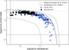 |
Fig. 1 BPT diagram of sample of spectra of Galactic and extragalactic H II regions and star-forming galaxies compiled in DESIRED-E used in this study. The dashed line represents the empirical relation by Kauffmann et al. (2003) that we have used to distinguish between starforming regions and active galactic nuclei (AGNs). The dotted curves and vertical and horizontal lines represent filters applied by Amayo et al. (2021) to extract photoionisation models to construct their ICF scheme for star-forming regions. |
3 Physical conditions and ionic abundances
We used PyNeb 1.1.18 (Luridiana et al. 2015; Morisset et al. 2020) with the atomic dataset presented in Table 1 and the H I effective recombination coefficients from Storey & Hummer (1995) to determine the physical conditions and the ionic abundances of the ionised nebulae. PyNeb is written in Python and is fully vectorised. To calculate the emissivity of collisional excitation lines, PyNeb calculates the relative population of the atomic levels of the ions by solving the statistical equilibrium equations. In the case of recombination lines, it interpolates the available emissivity tables.
References for atomic data used for collisionally excited lines.
3.1 Electron density
We used the getCrossTemDen routine of PyNeb to derive ne and Te of the sample objects. This routine cross-correlates the ne-sensitive diagnostics [S II] λ6731/λ6716, [O II] λ3726/λ3729, [Cl III] λ5538/λ5518, [Fe III] λ4658/λ4702, and [Ar IV]λ4740/ λ4711 with the Te-sensitive ones [N II]λ5755/λ6584, [O III]λ4363/λ5007, [Ar III] λ5192/λ7135, and [S III] λ6312/λ9069 using a Monte Carlo experiment generating 100 random values to propagate uncertainties in line inten-sities. This number was chosen as a compromise between calculation time and convergence of the result. As an output of this procedure, we obtain a set of ne and Te values along with their associated uncertainties for each diagnostic and individual point of the experiment. The average ne weighted by the inverse square of the error of the 100 individual points, is adopted as the representative value of the diagnostic. We used the Monte Carlo method to estimate the uncertainties in all physical-condition and ionic-abundance calculations. This is a well-suited procedure due to the complex and non-linear relationships between the various physical quantities – each one with its own uncertainty – involved in the calculations, especially for deriving ionic abundances.
Once we obtain the ne value of each diagnostic, we apply the criteria proposed by Méndez-Delgado et al. (2023a) to obtain a mean ne representative of each neb-ulae. If ne([S II] λ6731/λ6716) < 100 cm−3, we adopt ne = 100 ± 100 cm−3. If 100 cm−3 ≤ ne([S II] λ6731/λ6716) < 1000 cm−3, we adopt the average between ne([S II] λ6731/λ6716) and ne([O II] λ3726/λ3729). If ne([S II] λ6731/λ6716) ≥ 1000 cm−3, we adopt the average of ne([S II] λ6731/λ6716), ne([O II] λ3726/λ3729), ne([Cl III] λ5538/λ5518), ne([Fe III] λ4658/λ4702), and ne([Ar IV] λ4740/λ4711). In cases where a value of ne is not reported or could not be calculated in the source references, we adopt ne = 100 ± 100 cm−3. The adopted values of ne for each spectra used are given in Table A.2.
3.2 A representative electron temperature for the Cl2+ zone
We estimated Te([N II] λ5755/λ6584), Te([O III] λ4363/λ5007), and Te([S III] λ6312/λ9069) using the getTemDen routine of PyNeb and the aforementioned adopted average ne of each object. We also used a Monte Carlo experiment of 100 random values to propagate uncertainties in ne and line intensities ratios involved in the Te diagnostics. To ensure a good determination of Te for each object, we verified that the flux of the pairs of nebular lines coming from the same upper atomic level used (e.g. [O III] λλ5007, 4959, [S III] λλ9531, 9069, [N II] λλ6584, 6548) fit with their theoretical predictions (Storey & Zeippen 2000). We discard any diagnostic when the observed nebular line-intensity ratios differ by more than 20% from the theoretical values. There may be deviations from the theoretical [S III] λλ9531, 9069 ratio in a given object due to contamination of telluric absorption bands (for a discussion about this issue see Méndez-Delgado et al. 2024). There are a few objects where only one of the lines of the aforementioned pairs of nebular lines is reported. In these cases, we consider the single nebular line observed in the calculation, assuming that the Te derived is valid.
There is not a Te diagnostic based on [Cl III] lines, so we have to assume a Te value representative of the nebular zone where Cl2+ ion lies. This ion can be ionised by photons with energies between 23.81 and 39.61 eV. In Fig. 2 we compare the ionisation ranges of the lower ionic species of Cl, N, O, and S. We can see that the ionisation ranges of Cl2+ and S2+ (22.3 − 34.8 eV) are the most similar ones, so assuming Te(Cl2+) ≈ Te([S III]) seems to be a reasonable approximation.
We used the results from photoionisation models to check which of the Te diagnostics available, Te([N II]), Te([S III]), and Te([O III]) –or a combination of them– better reproduces the behaviour of Te(Cl2+) in order to obtain more precise Cl2+ abundances. To do that, we used the models of giant H II regions from the Mexican Million Models database1 (Morisset et al. 2015) under the ‘BOND’ reference (Vale Asari et al. 2016), built with Cloudy v17.01 (Ferland et al. 2017). We applied the same selection criteria as Amayo et al. (2021) to select the appropriate subset of models. These criteria are: (a) starburst ages lower than 6 Myr; (b) ionisation bounded nebulae and density bounded ones selected by a cut of 70 per cent of the Hβ flux; (c) a selection of realistic N/O, U, and O/H values (Vale Asari et al. 2016); (d) the application of H II region filters on the BPT diagram defined in Eq. (3) of Amayo et al. (2021, see Fig. 1). The final total number of individual models considered is 13 558.
In Fig. 3, we show the distribution of Te(Cl2+) as a function of Te(N+), Te(S2+), and Te(O2+) obtained from the photoionisation models. Each point represents the result of an individual model colour-coded by its mean ionisation degree, parameterised by the O2+/O ratio. The continuous red lines represent the linear least-squares fit to the points. Each panel has a small box below where we represent the standard deviation, σ, of the model points with respect to the fit as a function of Te. Figure 3 clearly indicates that when attending to photoionisation models Te(S2+) is the best proxy of Te(Cl2+) for typical spectra of H II regions. In fact, the mean σ of the Te(Cl2+) versus Te(S2+) is the lowest of the three panels represented in Fig. 3.
In Table 2, we collect the number of objects in our DESIRED-E sample with the different combinations of the three temperature diagnostics considered, Te([N II]), Te([S III]), and Te([O III]). Only 41% of the objects have Te([S III]). In order to obtain a better determination of the Cl2+ abundance in objects where we lack Te([S III]) and following suggestions by Domínguez-Guzmán et al. (2019), we defined a new Te indicator more representative of Te(Cl2+) than Te([N II]) or Te([O III]) alone, Trep, which, in the case of the models, is
![Mathematical equation: \[{T_{{\rm{rep}}}} = {T_{\rm{e}}}({{\rm{N}}^{\rm{ + }}})\cdot\left( {1 - \frac{{{O^{2 + }}}}{O}} \right) + {T_{\rm{e}}}({{\rm{O}}^{{\rm{2 + }}}})\cdot\frac{{{O^{2 + }}}}{O};\]](/articles/aa/full_html/2025/05/aa53950-25/aa53950-25-eq1.png) (1)
(1)
in the case of the observations, it is
![Mathematical equation: \[{T_{{\rm{rep}}}} = {T_{\rm{e}}}([{\rm{N}}{\mkern 1mu} {\rm{II}}])\cdot\left( {1 - \frac{{{O^{2 + }}}}{O}} \right) + {T_{\rm{e}}}([{\rm{O}}{\mkern 1mu} {\rm{III}}])\cdot\frac{{{O^{2 + }}}}{O}.\]](/articles/aa/full_html/2025/05/aa53950-25/aa53950-25-eq2.png) (2)
(2)
Trep takes into account the fact that the zone of an ionised nebula where Cl2+ lies should be intermediate to those of N+ and O2+. We weighted the contribution of the N+ and O2+ zones to Trep using the mean O2+/O ratio of the object. In Fig. 4, we can see that the mean σ of the model points around the fit is lower than in the Te(Cl2+) versus Te(N+) or Te(Cl2+) versus Te(O2+) relations separately. Table 2 indicates that 7.8 and 32.2% of the objects have only Te([N II]) or Te([O III]) determinations available. In these cases, we also applied Trep, but estimating the missing Te indicator using the relationship between Te([N II]) and Te([O III]) proposed by Garnett (1992). The different Te indicators derived for all the spectra used in this work are given in Table A.2.
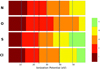 |
Fig. 2 Ionisation energies of different ionic species of N, O, S, and Cl we can find in usual ionisation conditions of star-forming regions. The vertical dotted black lines represent the range of photon energies capable to produce Cl2+ ions. |
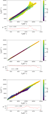 |
Fig. 3 Te(Cl2+) as a function of Te(N+) (top), Te(S2+) (middle), and Te(O2+) (bottom) obtained from the photoionisation models described in the text. Each point represents an individual model colour-coded by its mean ionisation degree, parameterised by the O2+/O ratio. The red line is a linear fit to the points. The small panels represent the values of σ to the fit in 1000 K bins. The mean σ is shown inside the panels. |
Available Te determinations for the sample objects and proxies to Te(Cl2+) for Cl2+/H+ calculation.
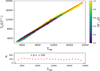 |
Fig. 4 Te(Cl2+) as a function of Trep obtained from the photoionisation models described in the text. The different elements of the diagram are described in Fig. 3. |
3.3 Ionic abundances
After adopting a value of ne and calculating the different Te indicators for the sample spectra – including Trep for those lacking Te([S III]) – we can proceed to calculating ionic abundances. In this work, we determined the abundances of O+, O2+, S+, S2+, Cl+, Cl2+, Cl3+, Ar2+, and Ar3+ ionic species. For O+, we used the [O II] λλ3727, 3729 doublet and the sum of the auroral lines [O II] λλ7319, 7320, 7330, 7331 when the bluer [O II] doublet lines were not available. In the case of O2+, we used the sum of the bright [O III] λλ4959, 5007 nebular lines. For S+ and S2+, we used the sum of [S II] λλ6716, 6731 and [S III] λλ9069, 9531 doublets, respectively. There are spectra that do not cover the near-IR range, so in such cases we used the [S III] λ6312 line to derive the S2+ abundance. For Cl2+, we used the sum of the [Cl III] doublet at 5517 and 5537 Å or one of those lines when the other is not detected. In a few objects, it is possible to obtain Cl+ and Cl3+ abundances, which can be calculated from [Cl II] 9123 Å and [Cl IV] 8046 Å lines, respectively. In the case of Ar2+, we used the [Ar III] λ7136 line alone, or in combination with [Ar III] λ7751 when both lines were available. Finally, we used the [Ar IV] λλ4711, 4740 doublet to derive the Ar3+ abundance.
We introduced Te([N II]) and the adopted ne in the getIonAbundance routine of PyNeb to calculate the abundance of low-ionisation ions such as O+, S+, and Cl+, propagating the uncertainties through 100-point Monte Carlo experiments. When Te([N II]) was not available for a given spectrum or the first diagnostic was unavailable, we applied the Te relations of Garnett (1992) to estimate it from Te([O III]) or Te([S III]). O2+, Cl3+, and Ar3+ abundances are determined using Te([O III]) and the adopted value of ne. In the spectra where Te([O III]) cannot be calculated, we used the Te relations of Garnett (1992) along with the values of Te([N II]) and/or Te([S III]) when one of these was determined from the spectra. The abundance of the intermediateionisation ions, S2+ and Ar2+, was calculated using the adopted value of ne and Te([S III]) or Te([N II]) or Te([O III]) along with the Te relations of Garnett (1992) when Te([S III]) is not available. Finally, as it is described in Sect. 3.2, the Cl2+ abundance is determined using Te([S III]) or Trep. The O+, O2+, S+, S2+, Cl2+, Ar2+, and Ar3+ abundances determined for all the spectra included in this study are collected in Table A.3. The Cl+ and Cl3+ abundances in the objects where it is possible to calculate them – along with their corresponding Cl2+ ones – are shown separately in Table 3.
Ionic and total Cl abundances for objects where [Cl II] and/or [Cl IV] lines are detected.
4 Total abundances
4.1 O, S, and Ar abundances
The total O abundances have been calculated as the sum of the O+/H+ and O2+/H+ ratios. Spectroscopic studies of metal-poor H II regions and SFGs (e.g. Izotov & Thuan 1999; Berg et al. 2022; Domínguez-Guzmán et al. 2022) indicate that the contribution of O3+/H+ can be considered negligible compared to the typical errors of the total O/H ratio. Total S abundances are determined from the sum of the S+ and S2+ ones and applying an ICF; we only considered spectra where these two ionic abundances are available. We considered two ways to determine the total Ar abundance, when Ar2+ lines are the only ones available in the spectrum and when we measure Ar2+ and Ar3+ lines, obviously the ICF used is different in each of these two cases.
Esteban et al. (2025) carried out a study on the abundance patterns of the alpha-elements Ne, S, and Ar based on the spectra of H II regions and SFGs compiled in DESIRED-E. We followed the same methodology to derive the S/H and Ar/H ratios for the objects analysed in this paper. After a critical examination of different ICF schemes, Esteban et al. (2025) found that the ICFs of Izotov et al. (2006) best represent the behaviour of the S and Ar abundance patterns in the types of objects we are concerned about. Izotov et al. (2006) used the photoionisation models of SFGs published by Stasińska & Izotov (2003), which used stellar energy distribution (SED) models from Starburst99 (Leitherer et al. 1999) as ionisation sources. The ICFs by Izotov et al. (2006) are parameterised by the ionisation degree and the metallicity of the nebulae. They provide three equations depending on metallicity: ‘low’ (12+log(O/H) ≤ 7.2), ‘intermediate’ (7.2 < 12+log(O/H) < 8.2), and ‘high’ (12+log(O/H) ≥ 8.2) ranges, which are used to interpolate the appropriate value of the ICF using the O/H ratio calculated for each object. In the case of Ar, Izotov et al. (2006) obtained two different sets of equations: one when only Ar2+ abundance is available, and another when both Ar2+ and Ar3+ are available. The relations given by Izotov et al. (2006) for S and Ar are valid for values of O2+/O ≥ 0.2. The total O, S, and Ar abundances determined for all the spectra included in this study are collected in Table A.4.
4.2 Cl abundances
As stated in Sect. 1, Cl2+ is the ionisation state of Cl that presents the brightest emission lines in the optical spectrum of nebulae. Cl+ and Cl3+ also produce optical CELs, but are much weaker, and they are detected in only a handful of objects. Only eight of the spectra of H II regions and SFGs with Cl2+ abundances of DESIRED-E that we used in our analysis2 have determinations of Cl+/H+ and 18 of Cl3+/H+ ratios. They are listed in Table 3. Of those objects, only six have both Cl+ and Cl3+ abundances.
For most of the objects with Cl+ and/or Cl3+ included in Table 3, we can derive the total Cl abundance without using an ICF(Cl)3. Considering the ionisation degree of the objects and the previous results of Esteban et al. (2015), we can obtain Cl/H as the sum of Cl+/H+ and Cl2+/H+ when O2+/O ≲ 0.30, as in the case of the Galactic H II regions M8 and Sh 2-311. We can derive Cl/H from the sum of Cl+/H+, Cl2+/H+, and Cl3+/H+ for the H II regions: Orion Nebula, NGC 2579, NGC 3576, and NGC 3603 in the Milky Way, and N44C and N66A in the Large and Small Magellanic Cloud (LMC and SMC), respectively. Finally, we can obtain Cl/H from the sum of Cl2+/H+ and Cl3+/H+ in the case of the high-ionisation-degree extragalactic H II regions: 30 Dor, Hubble V (NGC 6822), NGC 1714, NGC 5408, N81, and N88A; and for the SFGs HS1851+6933, Mrk 71, SHOC133, SBS 1420+540, Tol 1924−416, and W1702+18. All these highionisation objects show O2+/O ≳ 0.80, and we do not expect a significant fraction of Cl+ in them. The total Cl abundances determined from the sum of ionic abundances of all the afore-mentioned objects are given in Table 3.
For the objects where only the Cl2+ abundance is available or Cl/H cannot be derived from the ionic abundances observed, the Cl/O ratio has been determined applying the following relation:
![Mathematical equation: \[\frac{{{\rm{Cl}}}}{{\rm{O}}} = \frac{{{\rm{C}}{{\rm{l}}^{{\rm{2 + }}}}}}{{{{\rm{O}}^{{\rm{2 + }}}}}}\cdot{\rm{ICF}}({\rm{Cl}}).\]](/articles/aa/full_html/2025/05/aa53950-25/aa53950-25-eq105.png) (3)
(3)
We used two ICF(Cl)4 schemes to derive the total Cl abundance. The first set is the one by Izotov et al. (2006) described in Sect. 4.1, and the second one is the scheme proposed by Amayo et al. (2021). Esteban et al. (2025) described and analysed the suitability of these sets of ICFs in the case of Ne, S, and Ar (see footnote 2 in Esteban et al. (2025) for the convention used to name these ICFs). The ICFs by Amayo et al. (2021) are based on the same photoionisation models and selection criteria that we used to build the Te relations presented in Sect. 3.2. This ICF(Cl) can be applied for the entire range of the O2+/O ratio. The total Cl abundance determined for all the spectra included in this study, using the ICFs by Amayo et al. (2021) and Izotov et al. (2006), are collected in Table A.4.
In Fig. 5, we plot log(Cl2+/O2+) as a function of O2+/O for the H II regions and SFGs of the DESIRED-E sample. The coloured curves represent the different ICF(Cl) values defined by Eq. (3) provided by the schemes considered: Amayo et al. (2021, red dashed-dotted lines) and Izotov et al. (2006, dotted lines with colours corresponding to the three metallicity ranges). The horizontal dashed black line indicates the solar log(Cl/O) – along with its uncertainty represented by the grey band – as reference. This solar value has been calculated using the present-day Solar System Cl/H and the solar O/H ratios recommended by Lodders & Fegley (2023) and Asplund et al. (2021), respectively (this choice is justified at the end of this section). Figure 5 shows that the ICF(Cl) by Izotov et al. (2006) seems to better reproduce the behaviour of log(Cl2+/O2+) for objects with O2+/O > 0.8 (mostly SFGs). In Fig. 6, we show the difference of 12+log(Cl/H) cal-culated for all the sample objects using the ICF(Cl) schemes by Amayo et al. (2021) and Izotov et al. (2006). The Cl abundances determined from both ICFs begin to differ significantly when O2+/O > 0.8, with those calculated with the IFC(Cl) by Izotov et al. (2006) always being higher.
In Fig. 7, we show the log(Cl/O) values obtained with the two ICF(Cl) schemes used to obtain the total Cl abundances of our sample of DESIRED-E H II regions and SFGs. We represent log(Cl/O) as a function of O2+/O (right panels) and 12+log(O/H) (left panels). The number of spectra included in each panel of Fig. 7 depends on the ICF(Cl) scheme used. This is because the range of O2+/O ratios to which each scheme is applicable is different. The top panels represent the results using the ICF(Cl) by Amayo et al. (2021) and include 2825 spectra, 52.1% of them corresponding to H II regions and 47.9% to SFGs. The bottom panels of Fig. 7 show the results obtained using the ICF(Cl) by Izotov et al. (2006); in this case, the total number of objects represented is 263, with 48.7% of them corresponding to H II regions and 51.3% to SFGs. As in the top panels, we only include one spectrum of the Orion Nebula.
In Fig. 7, we represent the mean value of log(Cl/O) in four or five bins (orange diamonds) for values of 12+log(O/H) from 7.2 to 8.7 (bins 0.32 dex wide) and for O2+/O values from 0.0 to 1.0 in the top panels and from 0.2 to 1.0 in the bottom ones (bins 0.2 wide). The top right panel indicates that the log(Cl/O) determined using the ICF(Cl) by Amayo et al. (2021) becomes lower at higher O2+/O ratios. In fact, the mean value of log(Cl/O) of the bins decreases continuously. From the second bin (centred at O2+/O = 0.3) to the last one on the right, the difference of the mean value of log(Cl/O) of the bins is about 0.26 dex. This trend is clearly an artefact introduced by the ICF(Cl). Considering that O/H and O2+/O show a rough relation in H II regions and SFGs of DESIRED-E (see Fig. B.1 of Esteban et al. 2025), it is quite likely that the apparent increase of 0.21 dex in log(Cl/O) as 12+log(O/H) increases from 7.6 to 8.7 (top left panel of Fig. 7) is also actually an artefact produced by the ICF(Cl).
In the two bottom panels of Fig. 7, we represent the log(Cl/O) values obtained using the ICF(Cl) scheme by Izotov et al. (2006). The log(Cl/O) versus O2+/O distribution (bottom right panel) shows a quite flatter general behaviour. Log(Cl/O) does not show a systematic trend, and the maximum difference between the bins represented in the panel is only of about 0.11 dex. The only remarkable feature is the systematically higher log(Cl/O) values of the objects with O2+/O > 0.9. This is because the ICF(Cl) by Izotov et al. (2006) in that area varies very drastically – as can be seen in Fig. 5 – with the O2+/O ratio. Any fluctuation in the Cl2+ abundance is amplified and can produce odd Cl/H values. The log(Cl/O) versus 12+log(O/H) distribution obtained using the ICF(Cl) by Izotov et al. (2006) is also rather flat. The data points are distributed following a slightly curved distribution with a concave shape (looking from positive ordinates). From the second bin6, centred at 12+log(O/H) = 7.6, to the last one on the right, the maximum difference of the mean value of log(Cl/O) of the bins is only about 0.08 dex. Therefore, the use of the ICF(Cl) by Izotov et al. (2006) provides a rather flat log(Cl/O) distribution if we represent it as a function of 12+log(O/H) or O2+/O and as long as we restrict ourselves to O2+/O values between 0.2 and 0.9.
A more direct way to check which ICF(Cl) works best is to compare the Cl abundances provided by each ICF(Cl) scheme with the values obtained summing the ionic abundances of the objects included in Table 3. In Fig. 8, we make such comparison with the data points colour-coded by its O2+/O ratio. The diagrams show that both ICF(Cl) provide quite accurate values, with differences not larger than 0.1 dex except for a few highionisation-degree objects. In the case of the ICF(Cl) of Amayo et al. (2021), the slope of the linear fit is 0.86, providing lower Cl/H values at low metallicities and slightly higher at higher metallicities. The ICF(Cl) of Izotov et al. (2006) gives a linear fit with a slope of 0.98, which is practically parallel to the 1:1 relation, but with a very small shift of about 0.03 dex; this is with regard to obtaining slightly larger Cl/H ratios when using this ICF(Cl) and independently of the O2+/O ratio. It is important to remark that most of the low-metallicity objects with very large O2+/O ratios show the largest deviations with respect to the linear fit in the right panel of Fig. 8. This is due to the steep slope of the curve describing the Izotov ICF(Cl) at O2+/O > 0.90 (see Fig. 5), which, as we said before, can amplify the Cl/H ratio at values that are too high. We have recalculated the linear fit in the right panel without considering the objects with O2+/O > 0.90, in this case the shift disappears and the slope becomes 0.92.
The mean log(Cl/O) of all the data points represented in Fig. 7 is −3.55 ± 0.19 or −3.50 ± 0.18 when using the ICF(Cl) by Amayo et al. (2021) or Izotov et al. (2006), respectively. The solar log(Cl/O) recommended by Asplund et al. (2021) is −3.38 ± 0.21, and the one obtained from the Solar System Cl and O abundances recommended by Lodders & Fegley (2023) and Lodders (2021) is −3.50 ± 0.09. As can be seen, the two mean log(Cl/O) values we obtain are lower than the recommended solar one by Asplund et al. (2021) and clearly more consistent with the one obtained from the Solar System data by Lodders & Fegley (2023) and Lodders (2021), especially the log(Cl/O) obtained using the ICF(Cl) by Izotov et al. (2006). As discussed in Sect. 1, since the solar Cl/H ratio recommended by Asplund et al. (2021) comes from the sunspot determination by Maas et al. (2016), these same authors claim that their calculation is not entirely reliable because it does not consider radiative transfer effects. We applied the same criterion as Maas et al. (2016) in assuming the meteoritic Cl/H ratio as the most representative of the solar Cl abundance. In our case, the most recent determination of Cl/H = 5.23 ± 0.06 from CI-chondrites was obtained by Lodders & Fegley (2023). As Esteban et al. (2025) did in their study on the abundance patterns of alpha-elements in the DESIRED-E sample, we adopted the values recommended by Asplund et al. (2021) for the solar O/H, S/H, and Ar/H ratios.
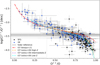 |
Fig. 5 Log(Cl2+/O2+) as function of ionisation degree, O2+/O, for H II regions (blue circles) and SFGs (black squares) of our DESIRED-E sample. The dashed black line and the grey band show the Solar System log(Cl/O) and its associated uncertainty obtained from the Solar System Cl/H ratio recommended by Lodders & Fegley (2023) and solar O/H ratio proposed by Asplund et al. (2021). The different curves represent the ICF schemes used in this study: Amayo et al. (2021, dashed-dotted red lines) and Izotov et al. (2006, dotted lines with colours corresponding to three metallicity ranges). |
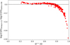 |
Fig. 6 Difference between logarithmic Cl abundances calculated from the spectra of our DESIRED-E sample using the ICF(Cl) schemes by Amayo et al. (2021) and Izotov et al. (2006). |
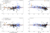 |
Fig. 7 Log(Cl/O) as function of 12+log(O/H) (left) and ionisation degree, O2+/O (right), for 280 (top panels) and 261 (bottom panels) of a sample of DESIRED-E objects. The fraction of the objects classified as H II regions or SFGs each represent about 50% of the sample. Top panels represent log(Cl/O) ratios calculated using the ICF(Cl) scheme by Amayo et al. (2021), and the bottom panels show those obtained using the ICF(Cl) by Izotov et al. (2006). The dotted red line represents the mean value of the log(Cl/O) obtained using each ICF(Cl). The orange diamonds indicate the mean log(Cl/O) values considering bins in 12+log(O/H) or O2+/O. The dashed black lines and grey bands are obtained from the solar 12+log(O/H) and Solar System log(Cl/H) ratios and their associated uncertainties recommended by Asplund et al. (2021) and Lodders & Fegley (2023), respectively. |
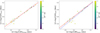 |
Fig. 8 Comparison of total Cl abundances obtained with and without ICF(Cl) for objects where Cl+ and/or Cl3+ abundances have been derived. Left and right panels show the results obtained when the Cl/H ratio is obtained using the ICF(Cl) by Amayo et al. (2021) or Izotov et al. (2006), respectively. Each data point is colour-coded by its ionisation degree and parameterised by the O2+/O ratio. The dotted line indicates the 1:1 relation. The red line in the left panel represents the linear fit to the data points. In the right panel, the dashed blue line represents the linear fit to all objects, and the solid red line represents the fit excluding objects with O2+/O > 0.9. |
5 The Cl/O, Cl/S, and Cl/Ar abundance ratios in the local Universe
According to the results obtained in Sect. 4.2, the ICF(Cl) by Izotov et al. (2006) provides a better match with the Cl/H ratios obtained from the sum of ionic abundances, a flatter log(Cl/O) versus O2+/O distribution, and a mean log(Cl/O) more consistent with the reference Cl/O ratio obtained from the Solar System Cl abundance recommended by Lodders & Fegley (2023) and the O abundance recommended by Asplund et al. (2021). We adopt the Cl abundances set obtained using the ICF(Cl) by Izotov et al. (2006) but excluding objects with O2+/O > 0.90 throughout the discussion that follows.
5.1 Cl/O
In Fig. 9, we represent the log(Cl/O) versus 12+log(O/H) distribution of SFGs and H II regions of the DESIRED-E sample, for which Cl/O ratios have been calculated using the ICF(Cl) scheme by Izotov et al. (2006). We also include the limited number of Cl/O ratio determinations available from stellar observations. The stellar Cl abundance is determined from spectral features of the HCl molecule in the L-band spectra of cold stars (Te f f < 4000 K). Using this method, Maas et al. (2016) and Maas & Pilachowski (2021) obtained data for several tens of M-type giants and one dwarf, which are shown as yellow stars in Fig. 9. The stars studied by Maas et al. (2016) and Maas & Pilachowski (2021) are located at distances of <1 Kpc and belong to the disc population, so most of the M-type giants of their sample must correspond to low-to-intermediate-mass stars with ages typically ranging from 1–5 Gyr (Martig et al. 2016; Miglio et al. 2021). Taking into account the prescriptions on the nucleosynthetic origin of O and Cl, the stars for which abundance data are included in Fig. 9 are not expected to have altered their initial amount of O and Cl since their formation. Therefore, their abundances should be representative of that of the ISM at the time when the stars were formed.
In Fig. 9, we can see that an important fraction of the stars show higher O/H ratios than most metallic H II regions. This is a well-known fact. Studies comparing nebular O abundances with those of their associated O- and B-type stars in Galactic starforming regions find average differences of about 0.2 dex (e.g. Simón-Díaz et al. 2006; Simón-Díaz & Stasińska 2011; García-Rojas et al. 2014), with stellar abundances being higher than nebular abundances when the latter are calculated using CELs. This offset is the so-called abundance discrepancy problem and may be related to the presence of fluctuations in the internal spatial distribution of Te in the ionised nebulae (Peimbert 1967; García-Rojas et al. 2007; Méndez-Delgado et al. 2023b). Although temperature fluctuations can alter the abundances calculated with CELs with respect to the true ones, the abundance ratios remain practically unchanged, so we do not expect an offset between stellar and nebular log(Cl/O) distributions (e.g. Esteban et al. 2020; Méndez-Delgado et al. 2024). The sample of M-type stars included in Fig. 9 provides a mean log(Cl/O) = −3.57 ± 0.16, which is slightly lower than the nebular value of −3.50 ± 0.18, but consistent considering the standard deviation of both quantities. The value of the reference Cl/O ratio we adopt for the Sun is −3.46 ± 0.07.
We performed a linear fit to the log(Cl/O) versus 12+log(O/H) distribution of the data for H II regions and SFGs represented in Fig. 9. The parameters of the fit are given in Table 4. We can see that the slope of the fit, 0.018 0.044, is very small and consistent with a flat distribution considering its uncertainty. Moreover, the sample Pearson correlation coefficient of the fit is also extremely low (0.023) and its large p value (0.729) indicates the absence of correlation between the variables involved in the linear fit7. Therefore, the Cl/O versus O distribution defined by the DESIRED-E objects shows a definitively flat behaviour. If we separate the objects according to their type (H II regions or SFGs), we also find no clear indication of an evolution of the Cl/O ratio as their average metallicity increases. The average O abundance of the H II regions included in Fig. 9 is 8.36 ± 0.18 while that of the SFGs is 8.10 ± 0.22. However, the mean log(Cl/O) for both types of objects is quite similar: −3.51 ± 0.15 and −3.55 ± 0.19, respectively.
A basically flat distribution of the Cl/O ratio as a function of metallicity is the common result in previous works devoted to derive chemical abundances in H II regions and SFGs. Izotov et al. (2006) presented the most extensive study until the present work, including the determination of Cl abundances for 148 SFGs. Those authors found a mean Cl/O ratio in agreement with the solar value and no significant trends in the log(Cl/O) versus 12+log(O/H) distribution; it was, however, but consistent with a linear fit with a slope of 0.120 ± 0.106. There are some other works dedicated to studying the behaviour of H II regions in external galaxies, but they are limited to a few tens of objects at most (and a quite narrow O/H baseline), which also show a Cl/O behaviour independent of metallicity and with mean Cl/O ratios similar to the solar one (e.g. Esteban et al. 2020; Rogers et al. 2022; Domínguez-Guzmán et al. 2022). Finally, the 15 local SFGs with enhanced star-formation rates studied by Arellano-Córdova et al. (2024) exhibit a constant trend of Cl/O with metallicity but somewhat subsolar Cl/O ratios and a mean value of log(Cl/O) = − 3.62 ± 0.17. Maas & Pilachowski (2021) also found a correlation between the O and Cl abundances as well as constant Cl/Ca ratios – Ca is another alpha-element – from spectral features of HCl molecule in nearby M giant and dwarf stars, indicating that Cl is made in similar nucleosynthesis sites as Ca or O. However, the stellar abundance ratios of Maas & Pilachowski (2021) show significant scatter.
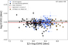 |
Fig. 9 log(Cl/O) as function of 12+log(O/H). Black squares and blue circles represent SFGs and H II regions of the DESIRED-E sample, for which Cl/O ratios have been calculated using the ICF(Cl) scheme by Izotov et al. (2006). Yellow stars represent the abundances obtained by Maas et al. (2016) and Maas & Pilachowski (2021) from spectral features of the HCl molecule in the L-band spectra of nearby M-giant and dwarf stars. The dashed black lines and grey bands are obtained from the solar 12+log(O/H) and Solar System log(Cl/H) ratios and their associated uncertainties recommended by Asplund et al. (2021) and Lodders & Fegley (2023), respectively. |
Linear fits log(Cl/X) = m × [12+log(X/H)] + n per element X.
5.2 Cl/S
35Cl is the most abundant stable isotope of Cl. It is mainly produced by proton capture on a 34S nucleus formed during oxygen burning (Clayton 2003). In Fig. 10, we show the log(Cl/S) versus 12+log(S/H) distribution of 229 SFGs and H II regions of the DESIRED-E sample, for which Cl and S abundances have been calculated using the ICF(Cl) and ICF(S) schemes by Izotov et al. (2006). A comprehensive analysis of the abundance patterns of S in DESIRED-E sample objects is presented in Esteban et al. (2025). Those authors find that while the log(S/O) versus 12+log(O/H) distribution of almost 1000 DESIRED-E spectra is rather flat, that of log(S/O) versus 12+log(S/H) shows a linear fit with a positive slope, this is compatible with some contribution of S from SNe Ia, as predicted by nucleosynthesis and chemical-evolution models (e.g. Iwamoto et al. 1999; Johnson 2019; Kobayashi et al. 2020). The linear fit to our log(Cl/S) versus 12+log(S/H) distribution (see Table 4) indicates a rather weak correlation (Pearson r coefficient = −0.209 and p = 0.00158) with a slightly negative slope ( −0.113 ± 0.032). The line fit is included in Fig. 10. The efficiency of the reaction where a 34S nucleus captures a proton to form 35Cl in stellar interiors is primarily determined based on its cross-section, which depends on factors such as temperature and density in the stellar nucleus (Lovely et al. 2021). The weak decrease in log(Cl/S) as 12+log(S/H) increases that we see in Fig. 10 could be due to a variation in the efficiency of the proton-capture reaction by 34S that produces 35Cl (the dominant isotopic species of Cl, see Maas & Pilachowski 2018) depending on the stellar metallicity. The chemical composition, in addition to varying the number of available nuclei, can alter the opacity of the stellar gas and vary the physical conditions in the stellar interior, such as the temperature gradient (e.g. Heger et al. 2003). The behaviour we observe in Fig. 10, although very weak, is very interesting and merits further study.
The mean log(Cl/S) of the objects included in Fig. 10 is −1.90 ± 0.18, which is in very good agreement with the reference value of −1.89 ± 0.07 we adopted for the Sun assuming the solar system Cl and solar S abundances recommended by Lodders & Fegley (2023) and Asplund et al. (2021), respectively. Separating the objects according to their type, we find exactly the same value of log(Cl/S) in both cases: 1.90, with a standard deviation of 0.17 and 0.20 in the case of H II regions and SFGs, respectively.
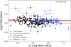 |
Fig. 10 log(Cl/S) as function of 12+log(S/H). Black squares and blue circles represent SFGs and H II regions of the DESIRED-E sample, for which Cl and S abundances have been calculated using the ICF scheme by Izotov et al. (2006). The dotted red line represents the mean log(Cl/S), while the solid one corresponds to the linear least-squares fit to the points. The dashed black lines and grey bands are obtained from the solar 12+log(S/H) and Solar System log(Cl/H) ratios and their associated uncertainties recommended by Asplund et al. (2021) and Lodders & Fegley (2023), respectively. |
5.3 Cl/Ar
The second stable isotope of Cl is 37Cl, which is two to four times less abundant than 35Cl (Maas & Pilachowski 2018). It is produced after the radioactive decay of 37Ar, formed by a single neutron capture by 36Ar, which in turn is a product of the oxygen burning in massive stars (Clayton 2003). Weak, slow neutron captures (s process) in massive stars can also produce 37Cl (Prantzos et al. 1990; Pignatari et al. 2010). In Fig. 11, we show the log(Cl/Ar) versus 12+log(Ar/H) distribution of the 211 H II regions and SFGs with Cl and Ar abundance determinations. Ar abundances have also been calculated using the ICF(Ar) scheme by Izotov et al. (2006). As in the case of S, an analysis of the abundance patterns of Ar in about 1000 star-forming regions of the local Universe is presented in Esteban et al. (2025). Those authors find that while log(Ar/O) decreases slightly as 12+log(O/H) increases, the log(Ar/O) versus 12+log(Ar/H) relation shows a small positive slope that might be due to a small contribution of Ar from SNe Ia. The linear-fit parameters given in Table 4 indicate the absence of correlation between log(Cl/Ar) and 12+log(Ar/H) and that their distribution is flat. The mean log(Cl/Ar) of the H II regions and SFGs included in Fig. 11 is −1.18 ± 0.16, which is consistent with the log(Cl/Ar) = −1.15 ± 0.07 we assume as representative for the Sun combin-ing the Solar System Cl abundance recommended by Lodders & Fegley (2023) and the solar Ar abundance proposed by Asplund et al. (2021). Finally, the mean log(Cl/Ar) obtained for H II regions is −1.20 ± 0.14, and it is −1.17 ± 0.18 for SFGs; this indicates the lack of significant evolution of this abundance ratio with metallicity.
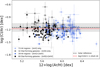 |
Fig. 11 log(Cl/Ar) as function of 12+log(Ar/H). Black squares and blue circles represent SFGs and H II regions of the DESIRED-E sample, for which Cl and Ar abundances have been calculated using the ICF scheme by Izotov et al. (2006). The dotted red line represents the mean log(Cl/Ar). The dashed black lines and grey bands are obtained from the solar 12+log(Ar/H) and Solar System log(Cl/H) ratios and their associated uncertainties recommended by Asplund et al. (2021) and Lodders & Fegley (2023), respectively. |
6 Conclusions
In this paper, we analyse the behaviour of the Cl abundance and its abundance ratios with respect to O, S, and Ar in more than 200 star-forming regions of the local Universe. We made use of the DEep Spectra of ionised REgions Database (DESIRED) Extended project (DESIRED-E; Méndez-Delgado et al. 2023a, 2024), which comprises more than 2000 spectra of H II regions and SFGs with direct determinations of electron temperature (Te). From this database, we selected spectra in which it is possible to determine the Cl2+ abundance and that are located below and to the left of the Kauffmann et al. (2003) line in the Baldwin-Phillips-Terlevich (BPT) diagram (Baldwin et al. 1981). We recalculated the physical conditions (ne and Te) and ionic abundances of Cl+, Cl2+, and Cl3+ for all spectra in a homogeneous manner. We used photoionisation models to explore the most representative Te diagnostics of the nebular zone where the Cl2+ ion lies. Our prescription for calculating more accurate Cl2+ abundances is to use Te([S III]) when it is available in the spectrum and a combination of Te([N II]) and Te([O III]) (Trep ) when the former is not available. Trep takes into account that the ionisation zone where Cl2+ is found is intermediate to that occupied by N+ and O2+.
We computed the total Cl abundance using the ICF(Cl) schemes by Amayo et al. (2021) and Izotov et al. (2006), as well as by simply summing the ionic abundances for nebulae where all the expected ionic species of Cl are observable. Our analysis indicates that the ICF scheme proposed by Izotov et al. (2006) better reproduces the observed distributions of the Cl/O ratio. It produces less dependent – flatter – distributions of the Cl/O ratios with respect to O2+/O and 12+log(O/H) and a mean log(Cl/O) value more consistent with our assumed solar value of −3.46 ± 0.07, which were derived using the Solar System Cl and solar O abundances recommended by Lodders & Fegley (2023) and Asplund et al. (2021), respectively. On the other hand, the comparison of the Cl abundance obtained with and without the use of the ICF(Cl) for objects in which the Cl/H ratio can be determined from the sum of ionic abundances shows a relationship closer to 1:1 in the case using the ICF(Cl) scheme by Izotov et al. (2006). Following the conclusions by Esteban et al. (2025), we also used the ICF schemes by Izotov et al. (2006) to calculate total S and Ar abundances.
We compared the nebular Cl/O distribution with stellar determinations and explored the behaviour of log(Cl/O) as a function of 12+log(O/H) for 237 DESIRED-E spectra; of those, 52.7% correspond to H II regions and 47.3% to SFGs. We find that both quantities are not correlated, indicating a lockstep evolution of both elements. We also find the same behaviour for the log(Cl/Ar) versus 12+log(Ar/H) distribution of our 229 DESIRED-E spectra (51.1% HII regions and 48.9% SFGs) for which both elemental abundances can be calculated. In contrast, the log(Cl/S) versus 12+log(S/H) distribution of 211 DESIREDE spectra (53.6% HII regions and 46.4% SFGs) shows a rather weak correlation with a slight negative slope. This behaviour could be due to a variation with respect to stellar metallicity in the efficiency of the proton capture reaction by 34S that produces 35Cl, the most abundant isotopic species of Cl.
Data availability
The complete tables of references, physical conditions and chemical abundances for all the objects in our sample can be found at https://zenodo.org/records/15005957.
Acknowledgements
We acknowlege the anonymous referee for her/his valuable comments and suggestions. MOG, CE, JGR and ERR acknowledge financial support from the Agencia Estatal de Investigación of the Ministerio de Ciencia e Innovación (AEIMCINN) under grants “The internal structure of ionised nebulae and its effects in the determination of the chemical composition of the interstellar medium and the Universe” with reference PID2023-151648NB-I00 (DOI:10.13039/5011000110339). JGR also acknowledges financial support from the AEI-MCINN, under Severo Ochoa Centres of Excellence Programme 2020– 2023 (CEX2019-000920-S), and from grant”Planetary nebulae as the key to understanding binary stellar evolution” with reference PID-2022136653NA-I00 (DOI:http://dx.doi.org/10.13039/501100011033) funded by the Ministerio de Ciencia, Innovación y Universidades (MCIU/AEI) and by ERDF “A way of making Europe” of the European Union. JEMD acknowledges support from project UNAM DGAPA-PAPIIT IG 101025, Mexico.
Appendix A Referencesfor the spectroscopic data
The complete reference tables associated with Appendix A can be found at: https://zenodo.org/records/15005957. The references for the spectroscopic data are: Arellano-Córdova et al. (2021); Berg et al. (2013); Bresolin (2007); DelgadoInglada et al. (2016); Domínguez-Guzmán et al. (2022); Esteban et al. (2004, 2009, 2013, 2014, 2017, 2020); Esteban & García-Rojas (2018); Fernández et al. (2018, 2022); Fernández-Martín et al. (2017); García-Rojas et al. (2004, 2005, 2006, 2007); Guseva et al. (2000, 2003, 2009, 2011, 2024); Izotov et al. (1994, 1997, 2004, 2006, 2009, 2017, 2021); Izotov & Thuan (2004); Kurt et al. (1999); López-Sánchez et al. (2007); López-Sánchez & Esteban (2009); Méndez-Delgado et al. (2021a,b, 2022); Mesa-Delgado et al. (2009); Noeske et al. (2000); Peimbert et al. (1986, 2005, 2012); Peimbert (2003); Peña-Guerrero et al. (2012); Rogers et al. (2022); Skillman et al. (2003); Thuan et al. (1995); Thuan & Izotov (2005); Toribio San Cipriano et al. (2016); Valerdi et al. (2019, 2021); Zurita & Bresolin (2012)
References
- Amayo, A., Delgado-Inglada, G., & Stasi ńska, G. 2021, MNRAS, 505, 2361 [CrossRef] [Google Scholar]
- Arellano-Córdova, K. Z., Esteban, C., García-Rojas, J., & Méndez-Delgado, J. E. 2020, MNRAS, 496, 1051 [Google Scholar]
- Arellano-Córdova, K. Z., Esteban, C., García-Rojas, J., & Méndez-Delgado, J. E. 2021, MNRAS, 502, 225 [CrossRef] [Google Scholar]
- Arellano-Córdova, K. Z., Berg, D. A., Mingozzi, M., et al. 2024, ApJ, 968, 98 [Google Scholar]
- Asplund, M., Amarsi, A. M., & Grevesse, N. 2021, A&A, 653, A141 [NASA ADS] [CrossRef] [EDP Sciences] [Google Scholar]
- Baldwin, J. A., Phillips, M. M., & Terlevich, R. 1981, PASP, 93, 5 [Google Scholar]
- Berg, D. A., Skillman, E. D., Garnett, D. R., et al. 2013, ApJ, 775, 128 [NASA ADS] [CrossRef] [Google Scholar]
- Berg, D. A., James, B. L., King, T., et al. 2022, ApJS, 261, 31 [NASA ADS] [CrossRef] [Google Scholar]
- Bresolin, F. 2007, ApJ, 656, 186 [NASA ADS] [CrossRef] [Google Scholar]
- Butler, K., & Zeippen, C. J. 1989, A&A, 208, 337 [NASA ADS] [Google Scholar]
- Clayton, D. 2003, Handbook of Isotopes in the Cosmos (Cambridge University Press) [Google Scholar]
- Deb, N. C., & Hibbert, A. 2009, At. Data Nucl. Data Tables, 95, 184 [NASA ADS] [CrossRef] [Google Scholar]
- Delgado-Inglada, G., Morisset, C., & Stasi ńska, G. 2014, MNRAS, 440, 536 [NASA ADS] [CrossRef] [Google Scholar]
- Delgado-Inglada, G., Mesa-Delgado, A., García-Rojas, J., Rodríguez, M., & Esteban, C. 2016, MNRAS, 456, 3855 [NASA ADS] [CrossRef] [Google Scholar]
- Domínguez-Guzmán, G., Rodríguez, M., Esteban, C., & García-Rojas, J. 2019, arXiv e-prints, [arXiv:1906.02102] [Google Scholar]
- Domínguez-Guzmán, G., Rodríguez, M., García-Rojas, J., Esteban, C., & Toribio San Cipriano, L. 2022, MNRAS, 517, 4497 [CrossRef] [Google Scholar]
- Esteban, C., & García-Rojas, J. 2018, MNRAS, 478, 2315 [NASA ADS] [CrossRef] [Google Scholar]
- Esteban, C., Peimbert, M., García-Rojas, J., et al. 2004, MNRAS, 355, 229 [NASA ADS] [CrossRef] [Google Scholar]
- Esteban, C., Bresolin, F., Peimbert, M., et al. 2009, ApJ, 700, 654 [NASA ADS] [CrossRef] [Google Scholar]
- Esteban, C., Carigi, L., Copetti, M. V. F., et al. 2013, MNRAS, 433, 382 [NASA ADS] [CrossRef] [Google Scholar]
- Esteban, C., García-Rojas, J., Carigi, L., et al. 2014, MNRAS, 443, 624 [NASA ADS] [CrossRef] [Google Scholar]
- Esteban, C., García-Rojas, J., & Pérez-Mesa, V. 2015, MNRAS, 452, 1553 [NASA ADS] [CrossRef] [Google Scholar]
- Esteban, C., Fang, X., García-Rojas, J., & Toribio San Cipriano, L. 2017, MNRAS, 471, 987 [NASA ADS] [CrossRef] [Google Scholar]
- Esteban, C., Bresolin, F., García-Rojas, J., & Toribio San Cipriano, L. 2020, MNRAS, 491, 2137 [NASA ADS] [Google Scholar]
- Esteban, C., Méndez-Delgado, J. E., García-Rojas, J., et al. 2025, A&A, 697, A61 [NASA ADS] [CrossRef] [EDP Sciences] [Google Scholar]
- Faundez-Abans, M., & Maciel, W. J. 1987, Ap&SS, 129, 353 [Google Scholar]
- Ferland, G. J., Chatzikos, M., Guzmán, F., et al. 2017, Rev. Mexicana Astron. Astrofis., 53, 385 [Google Scholar]
- Fernández-Martín, A., Pérez-Montero, E., Vílchez, J. M., & Mampaso, A. 2017, A&A, 597, A84 [NASA ADS] [CrossRef] [EDP Sciences] [Google Scholar]
- Fernández, V., Terlevich, E., Díaz, A. I., Terlevich, R., & Rosales-Ortega, F. F. 2018, MNRAS, 478, 5301 [CrossRef] [Google Scholar]
- Fernández, V., Amorín, R., Pérez-Montero, E., et al. 2022, MNRAS, 511, 2515 [CrossRef] [Google Scholar]
- Fritzsche, S., Fricke, B., Geschke, D., Heitmann, A., & Sienkiewicz, J. E. 1999, ApJ, 518, 994 [NASA ADS] [CrossRef] [Google Scholar]
- Froese Fischer, C., & Tachiev, G. 2004, At. Data Nucl. Data Tables, 87, 1 [NASA ADS] [CrossRef] [Google Scholar]
- Froese Fischer, C., Tachiev, G., & Irimia, A. 2006, At. Data Nucl. Data Tables, 92, 607 [NASA ADS] [CrossRef] [Google Scholar]
- Galavis, M. E., Mendoza, C., & Zeippen, C. J. 1995, A&AS, 111, 347 [Google Scholar]
- García-Rojas, J., Esteban, C., Peimbert, M., et al. 2004, ApJS, 153, 501 [CrossRef] [Google Scholar]
- García-Rojas, J., Esteban, C., Peimbert, A., et al. 2005, MNRAS, 362, 301 [CrossRef] [Google Scholar]
- García-Rojas, J., Esteban, C., Peimbert, M., et al. 2006, MNRAS, 368, 253 [CrossRef] [Google Scholar]
- García-Rojas, J., Esteban, C., Peimbert, A., et al. 2007, Rev. Mexicana Astron. Astrofis., 43, 3 [Google Scholar]
- García-Rojas, J., Simón-Díaz, S., & Esteban, C. 2014, A&A, 571, A93 [NASA ADS] [CrossRef] [EDP Sciences] [Google Scholar]
- Garnett, D. R. 1992, AJ, 103, 1330 [NASA ADS] [CrossRef] [Google Scholar]
- Grieve, M. F. R., Ramsbottom, C. A., Hudson, C. E., & Keenan, F. P. 2014, ApJ, 780, 110 [Google Scholar]
- Guseva, N. G., Izotov, Y. I., & Thuan, T. X. 2000, ApJ, 531, 776 [NASA ADS] [CrossRef] [Google Scholar]
- Guseva, N. G., Papaderos, P., Izotov, Y. I., et al. 2003, A&A, 407, 105 [NASA ADS] [CrossRef] [EDP Sciences] [Google Scholar]
- Guseva, N. G., Papaderos, P., Meyer, H. T., Izotov, Y. I., & Fricke, K. J. 2009, A&A, 505, 63 [NASA ADS] [CrossRef] [EDP Sciences] [Google Scholar]
- Guseva, N. G., Izotov, Y. I., Stasi ńska, G., et al. 2011, A&A, 529, A149 [NASA ADS] [CrossRef] [EDP Sciences] [Google Scholar]
- Guseva, N. G., Thuan, T. X., & Izotov, Y. I. 2024, MNRAS, 527, 3932 [Google Scholar]
- Hall, D. N. B., & Noyes, R. W. 1972, ApJ, 175, L95 [Google Scholar]
- Heger, A., Fryer, C. L., Woosley, S. E., Langer, N., & Hartmann, D. H. 2003, ApJ, 591, 288 [CrossRef] [Google Scholar]
- Henry, R. B. C., Kwitter, K. B., & Balick, B. 2004, AJ, 127, 2284 [CrossRef] [Google Scholar]
- Irimia, A., & Froese Fischer, C. 2005, Phys. Scr, 71, 172 [NASA ADS] [CrossRef] [Google Scholar]
- Iwamoto, K., Brachwitz, F., Nomoto, K., et al. 1999, ApJS, 125, 439 [NASA ADS] [CrossRef] [Google Scholar]
- Izotov, Y. I., & Thuan, T. X. 1999, ApJ, 511, 639 [NASA ADS] [CrossRef] [Google Scholar]
- Izotov, Y. I., & Thuan, T. X. 2004, ApJ, 602, 200 [CrossRef] [Google Scholar]
- Izotov, Y. I., Thuan, T. X., & Lipovetsky, V. A. 1994, ApJ, 435, 647 [NASA ADS] [CrossRef] [Google Scholar]
- Izotov, Y. I., Thuan, T. X., & Lipovetsky, V. A. 1997, ApJS, 108, 1 [NASA ADS] [CrossRef] [Google Scholar]
- Izotov, Y. I., Papaderos, P., Guseva, N. G., Fricke, K. J., & Thuan, T. X. 2004, A&A, 421, 539 [NASA ADS] [CrossRef] [EDP Sciences] [Google Scholar]
- Izotov, Y. I., Stasi ńska, G., Meynet, G., Guseva, N. G., & Thuan, T. X. 2006, A&A, 448, 955 [CrossRef] [EDP Sciences] [Google Scholar]
- Izotov, Y. I., Guseva, N. G., Fricke, K. J., & Papaderos, P. 2009, A&A, 503, 61 [NASA ADS] [CrossRef] [EDP Sciences] [Google Scholar]
- Izotov, Y. I., Thuan, T. X., & Guseva, N. G. 2017, MNRAS, 471, 548 [NASA ADS] [CrossRef] [Google Scholar]
- Izotov, Y. I., Thuan, T. X., & Guseva, N. G. 2021, MNRAS, 508, 2556 [NASA ADS] [CrossRef] [Google Scholar]
- Jenkins, E. B. 2009, ApJ, 700, 1299 [Google Scholar]
- Johnson, J. A. 2019, Science, 363, 474 [Google Scholar]
- Kaufman, V., & Sugar, J. 1986, J. Phys. Chem. Ref. Data, 15, 321 [NASA ADS] [CrossRef] [Google Scholar]
- Kauffmann, G., Heckman, T. M., Tremonti, C., et al. 2003, MNRAS, 346, 1055 [Google Scholar]
- Kisielius, R., Storey, P. J., Ferland, G. J., & Keenan, F. P. 2009, MNRAS, 397, 903 [NASA ADS] [CrossRef] [Google Scholar]
- Kobayashi, C., Karakas, A. I., & Umeda, H. 2011, MNRAS, 414, 3231 [Google Scholar]
- Kobayashi, C., Karakas, A. I., & Lugaro, M. 2020, ApJ, 900, 179 [Google Scholar]
- Kurt, C. M., Dufour, R. J., Garnett, D. R., et al. 1999, ApJ, 518, 246 [Google Scholar]
- Leitherer, C., Schaerer, D., Goldader, J. D., et al. 1999, ApJS, 123, 3 [Google Scholar]
- Lodders, K. 2021, Space Sci. Rev., 217, 44 [NASA ADS] [CrossRef] [Google Scholar]
- Lodders, K., & Fegley, Bruce, J. 2023, Chem. Erde/Geochemistry, 83, 125957 [Google Scholar]
- Lodders, K., Palme, H., & Gail, H. P. 2009, Landolt Börnstein, 4B, 712 [Google Scholar]
- López-Sánchez, A. R., & Esteban, C. 2009, A&A, 508, 615 [NASA ADS] [CrossRef] [EDP Sciences] [Google Scholar]
- López-Sánchez, Á. R., Esteban, C., García-Rojas, J., Peimbert, M., & Rodríguez, M. 2007, ApJ, 656, 168 [CrossRef] [Google Scholar]
- Lovely, M., Lennarz, A., Connolly, D., et al. 2021, Phys. Rev. C, 103, 055801 [Google Scholar]
- Luridiana, V., Morisset, C., & Shaw, R. A. 2015, A&A, 573, A42 [NASA ADS] [CrossRef] [EDP Sciences] [Google Scholar]
- Maas, Z. G., & Pilachowski, C. A. 2018, AJ, 156, 2 [NASA ADS] [CrossRef] [Google Scholar]
- Maas, Z. G., & Pilachowski, C. A. 2021, AJ, 161, 183 [NASA ADS] [CrossRef] [Google Scholar]
- Maas, Z. G., Pilachowski, C. A., & Hinkle, K. 2016, AJ, 152, 196 [NASA ADS] [CrossRef] [Google Scholar]
- Maciel, W. J., & Chiappini, C. 1994, Ap&SS, 219, 231 [Google Scholar]
- Martig, M., Fouesneau, M., Rix, H.-W., et al. 2016, MNRAS, 456, 3655 [NASA ADS] [CrossRef] [Google Scholar]
- Mathis, J. S., & Rosa, M. R. 1991, A&A, 245, 625 [NASA ADS] [Google Scholar]
- Melnick, J., Terlevich, R., & Eggleton, P. P. 1985, MNRAS, 216, 255 [NASA ADS] [Google Scholar]
- Méndez-Delgado, J. E., Esteban, C., García-Rojas, J., et al. 2021a, MNRAS, 502, 1703 [Google Scholar]
- Méndez-Delgado, J. E., Henney, W. J., Esteban, C., et al. 2021b, ApJ, 918, 27 [Google Scholar]
- Méndez-Delgado, J. E., Esteban, C., García-Rojas, J., & Henney, W. J. 2022, MNRAS, 514, 744 [CrossRef] [Google Scholar]
- Méndez-Delgado, J. E., Esteban, C., García-Rojas, J., et al. 2023a, MNRAS, 523, 2952 [Google Scholar]
- Méndez-Delgado, J. E., Esteban, C., García-Rojas, J., Kreckel, K., & Peimbert, M. 2023b, Nature, 618, 249 [Google Scholar]
- Méndez-Delgado, J. E., Esteban, C., García-Rojas, J., Kreckel, K., & Peimbert, M. 2024, Nat. Astron., 8, 275 [Google Scholar]
- Mendoza, C. 1983, in IAU Symposium, 103, Planetary Nebulae, ed. L. H. Aller, 143 [NASA ADS] [Google Scholar]
- Mendoza, C., & Zeippen, C. J. 1982, MNRAS, 198, 127 [NASA ADS] [Google Scholar]
- Mendoza, C., & Zeippen, C. J. 1983, MNRAS, 202, 981 [NASA ADS] [CrossRef] [Google Scholar]
- Mendoza, C., Méndez-Delgado, J. E., Bautista, M., García-Rojas, J., & Morisset, C. 2023, Atoms, 11, 63 [NASA ADS] [CrossRef] [Google Scholar]
- Mesa-Delgado, A., Esteban, C., García-Rojas, J., et al. 2009, MNRAS, 395, 855 [NASA ADS] [CrossRef] [Google Scholar]
- Miglio, A., Chiappini, C., Mackereth, J. T., et al. 2021, A&A, 645, A85 [NASA ADS] [CrossRef] [EDP Sciences] [Google Scholar]
- Morisset, C., Delgado-Inglada, G., & Flores-Fajardo, N. 2015, Rev. Mexicana Astron. Astrofis., 51, 103 [NASA ADS] [Google Scholar]
- Morisset, C., Luridiana, V., García-Rojas, J., et al. 2020, Atoms, 8, 66 [NASA ADS] [CrossRef] [Google Scholar]
- Noeske, K. G., Guseva, N. G., Fricke, K. J., et al. 2000, A&A, 361, 33 [NASA ADS] [Google Scholar]
- Nomoto, K., Iwamoto, K., Nakasato, N., et al. 1997, Nucl. Phys. A, 621, 467 [NASA ADS] [CrossRef] [Google Scholar]
- Nomoto, K., Tominaga, N., Umeda, H., Kobayashi, C., & Maeda, K. 2006, Nucl. Phys. A, 777, 424 [CrossRef] [Google Scholar]
- Peimbert, M. 1967, ApJ, 150, 825 [NASA ADS] [CrossRef] [Google Scholar]
- Peimbert, A. 2003, ApJ, 584, 735 [NASA ADS] [CrossRef] [Google Scholar]
- Peimbert, M., & Torres-Peimbert, S. 1977, MNRAS, 179, 217 [NASA ADS] [Google Scholar]
- Peimbert, M., Pena, M., & Torres-Peimbert, S. 1986, A&A, 158, 266 [Google Scholar]
- Peimbert, A., Peimbert, M., & Ruiz, M. T. 2005, ApJ, 634, 1056 [NASA ADS] [CrossRef] [Google Scholar]
- Peimbert, A., Peña-Guerrero, M. A., & Peimbert, M. 2012, ApJ, 753, 39 [NASA ADS] [CrossRef] [Google Scholar]
- Peña-Guerrero, M. A., Peimbert, A., Peimbert, M., & Ruiz, M. T. 2012, ApJ, 746, 115 [CrossRef] [Google Scholar]
- Pignatari, M., Gallino, R., Heil, M., et al. 2010, ApJ, 710, 1557 [Google Scholar]
- Prantzos, N., Hashimoto, M., & Nomoto, K. 1990, A&A, 234, 211 [NASA ADS] [Google Scholar]
- Ramsbottom, C. A., & Bell, K. L. 1997, At. Data Nucl. Data Tables, 66, 65 [NASA ADS] [CrossRef] [Google Scholar]
- Rogers, N. S. J., Skillman, E. D., Pogge, R. W., et al. 2022, ApJ, 939, 44 [NASA ADS] [CrossRef] [Google Scholar]
- Sargent, W. L. W., & Searle, L. 1970, ApJ, 162, L155 [NASA ADS] [CrossRef] [Google Scholar]
- Simón-Díaz, S., & Stasi ńska, G. 2011, A&A, 526, A48 [CrossRef] [EDP Sciences] [Google Scholar]
- Simón-Díaz, S., Herrero, A., Esteban, C., & Najarro, F. 2006, A&A, 448, 351 [NASA ADS] [CrossRef] [EDP Sciences] [Google Scholar]
- Skillman, E. D., Côté, S., & Miller, B. W. 2003, AJ, 125, 610 [NASA ADS] [CrossRef] [Google Scholar]
- Stasi ńska, G., & Izotov, Y. 2003, A&A, 397, 71 [NASA ADS] [CrossRef] [EDP Sciences] [Google Scholar]
- Storey, P. J., & Hummer, D. G. 1995, MNRAS, 272, 41 [NASA ADS] [CrossRef] [Google Scholar]
- Storey, P. J., & Zeippen, C. J. 2000, MNRAS, 312, 813 [NASA ADS] [CrossRef] [Google Scholar]
- Storey, P. J., Sochi, T., & Badnell, N. R. 2014, MNRAS, 441, 3028 [CrossRef] [Google Scholar]
- Tayal, S. S. 2004, A&A, 426, 717 [NASA ADS] [CrossRef] [EDP Sciences] [Google Scholar]
- Tayal, S. S. 2011, ApJS, 195, 12 [Google Scholar]
- Tayal, S. S., & Zatsarinny, O. 2010, ApJS, 188, 32 [NASA ADS] [CrossRef] [Google Scholar]
- Telles, E., Melnick, J., & Terlevich, R. 1997, MNRAS, 288, 78 [CrossRef] [Google Scholar]
- Thuan, T. X., & Izotov, Y. I. 2005, ApJS, 161, 240 [NASA ADS] [CrossRef] [Google Scholar]
- Thuan, T. X., Izotov, Y. I., & Lipovetsky, V. A. 1995, ApJ, 445, 108 [NASA ADS] [CrossRef] [Google Scholar]
- Toribio San Cipriano, L., García-Rojas, J., Esteban, C., Bresolin, F., & Peimbert, M. 2016, MNRAS, 458, 1866 [NASA ADS] [CrossRef] [Google Scholar]
- Travaglio, C., Hillebrandt, W., Reinecke, M., & Thielemann, F. K. 2004, A&A, 425, 1029 [NASA ADS] [CrossRef] [EDP Sciences] [Google Scholar]
- Vale Asari, N., Stasi ńska, G., Morisset, C., & Cid Fernandes, R. 2016, MNRAS, 460, 1739 [NASA ADS] [CrossRef] [Google Scholar]
- Valerdi, M., Peimbert, A., Peimbert, M., & Sixtos, A. 2019, ApJ, 876, 98 [NASA ADS] [CrossRef] [Google Scholar]
- Valerdi, M., Peimbert, A., & Peimbert, M. 2021, MNRAS, 505, 3624 [NASA ADS] [CrossRef] [Google Scholar]
- Wallace, L., Hinkle, K., & Livingston, W. C. 2002, NSO Technical Report #02-001 (Tucson: National Solar Observatory) [Google Scholar]
- Wiese, W. L., Fuhr, J. R., & Deters, T. M. 1996, J. Phys. Chem. Ref. Data, Monogr., 7, 403 [Google Scholar]
- Woosley, S. E., & Weaver, T. A. 1995, ApJS, 101, 181 [Google Scholar]
- Woosley, S. E., Hartmann, D. H., Hoffman, R. D., & Haxton, W. C. 1990, ApJ, 356, 272 [NASA ADS] [CrossRef] [Google Scholar]
- Yokoyama, T., Nagashima, K., Nakai, I., et al. 2023, Science, 379, abn7850 [NASA ADS] [CrossRef] [Google Scholar]
- Zhang, H. 1996, A&AS, 119, 523 [NASA ADS] [CrossRef] [EDP Sciences] [Google Scholar]
- Zurita, A., & Bresolin, F. 2012, MNRAS, 427, 1463 [NASA ADS] [CrossRef] [Google Scholar]
We note that the total number of spectra with Cl2+ abundances is 294, but 12 of them correspond to different positions of the Orion Nebula. From now on, for subsequent analyses we only consider the slit position observed by Esteban et al. (2004) for this object.
It is interesting to comment that with the advent of the James Webb Space Telescope (JWST) and using the MIRI MRS spectrograph (5– 28 µm), it is possible to observe Cl+ and Cl3+ CELs in the mid-infrared (MIR, [Cl II] λ14.4 and [Cl IV] λλ 11.8, 20.3), although this spectral domain lacks Cl2+ lines, that is, the generally dominant ionic species in H II regions. In principle, by combining optical and MIR observations of the same object we could obtain total Cl abundances and even of S and Ar without ICFs if we detect [S IV]λ10.5 and [Ar II]λ6.9 lines. However, the combination of optical and MIR observations poses other types of problems, such as the aperture matching and relative flux calibration between both spectral ranges.
In the form we define this ICF, it should be expressed as ICF(Cl2+/O2+). We abbreviate it as ICF(Cl) for simplicity.
The number of objects represented in Fig. 7 is lower than in Fig. 5, because while in Fig. 5 we include all the spectra with Cl2+ abundance determinations, in Fig. 7 we only show one of the 13 spectra from the different areas of the Orion Nebula included in DESIRED-E (the one observed by Esteban et al. 2004).
The first bin contains too few data points, and several of them show high Cl/H ratios produced by the amplifying effect of the ICF(Cl) by Izotov et al. (2006) on objects with O2+/O > 0.9.
The p value is used to evaluate the plausibility of the null hypothesis. A value of p > 0.05 indicates that the null hypothesis is plausible; that is, there is not significant linear fit between the variables. On the other hand, when p ≤ 0.05 it can be said that there is a significant correlation between both variables.
All Tables
Available Te determinations for the sample objects and proxies to Te(Cl2+) for Cl2+/H+ calculation.
Ionic and total Cl abundances for objects where [Cl II] and/or [Cl IV] lines are detected.
All Figures
|
Fig. 1 BPT diagram of sample of spectra of Galactic and extragalactic H II regions and star-forming galaxies compiled in DESIRED-E used in this study. The dashed line represents the empirical relation by Kauffmann et al. (2003) that we have used to distinguish between starforming regions and active galactic nuclei (AGNs). The dotted curves and vertical and horizontal lines represent filters applied by Amayo et al. (2021) to extract photoionisation models to construct their ICF scheme for star-forming regions. |
| In the text | |
|
Fig. 2 Ionisation energies of different ionic species of N, O, S, and Cl we can find in usual ionisation conditions of star-forming regions. The vertical dotted black lines represent the range of photon energies capable to produce Cl2+ ions. |
| In the text | |
|
Fig. 3 Te(Cl2+) as a function of Te(N+) (top), Te(S2+) (middle), and Te(O2+) (bottom) obtained from the photoionisation models described in the text. Each point represents an individual model colour-coded by its mean ionisation degree, parameterised by the O2+/O ratio. The red line is a linear fit to the points. The small panels represent the values of σ to the fit in 1000 K bins. The mean σ is shown inside the panels. |
| In the text | |
|
Fig. 4 Te(Cl2+) as a function of Trep obtained from the photoionisation models described in the text. The different elements of the diagram are described in Fig. 3. |
| In the text | |
|
Fig. 5 Log(Cl2+/O2+) as function of ionisation degree, O2+/O, for H II regions (blue circles) and SFGs (black squares) of our DESIRED-E sample. The dashed black line and the grey band show the Solar System log(Cl/O) and its associated uncertainty obtained from the Solar System Cl/H ratio recommended by Lodders & Fegley (2023) and solar O/H ratio proposed by Asplund et al. (2021). The different curves represent the ICF schemes used in this study: Amayo et al. (2021, dashed-dotted red lines) and Izotov et al. (2006, dotted lines with colours corresponding to three metallicity ranges). |
| In the text | |
|
Fig. 6 Difference between logarithmic Cl abundances calculated from the spectra of our DESIRED-E sample using the ICF(Cl) schemes by Amayo et al. (2021) and Izotov et al. (2006). |
| In the text | |
|
Fig. 7 Log(Cl/O) as function of 12+log(O/H) (left) and ionisation degree, O2+/O (right), for 280 (top panels) and 261 (bottom panels) of a sample of DESIRED-E objects. The fraction of the objects classified as H II regions or SFGs each represent about 50% of the sample. Top panels represent log(Cl/O) ratios calculated using the ICF(Cl) scheme by Amayo et al. (2021), and the bottom panels show those obtained using the ICF(Cl) by Izotov et al. (2006). The dotted red line represents the mean value of the log(Cl/O) obtained using each ICF(Cl). The orange diamonds indicate the mean log(Cl/O) values considering bins in 12+log(O/H) or O2+/O. The dashed black lines and grey bands are obtained from the solar 12+log(O/H) and Solar System log(Cl/H) ratios and their associated uncertainties recommended by Asplund et al. (2021) and Lodders & Fegley (2023), respectively. |
| In the text | |
|
Fig. 8 Comparison of total Cl abundances obtained with and without ICF(Cl) for objects where Cl+ and/or Cl3+ abundances have been derived. Left and right panels show the results obtained when the Cl/H ratio is obtained using the ICF(Cl) by Amayo et al. (2021) or Izotov et al. (2006), respectively. Each data point is colour-coded by its ionisation degree and parameterised by the O2+/O ratio. The dotted line indicates the 1:1 relation. The red line in the left panel represents the linear fit to the data points. In the right panel, the dashed blue line represents the linear fit to all objects, and the solid red line represents the fit excluding objects with O2+/O > 0.9. |
| In the text | |
|
Fig. 9 log(Cl/O) as function of 12+log(O/H). Black squares and blue circles represent SFGs and H II regions of the DESIRED-E sample, for which Cl/O ratios have been calculated using the ICF(Cl) scheme by Izotov et al. (2006). Yellow stars represent the abundances obtained by Maas et al. (2016) and Maas & Pilachowski (2021) from spectral features of the HCl molecule in the L-band spectra of nearby M-giant and dwarf stars. The dashed black lines and grey bands are obtained from the solar 12+log(O/H) and Solar System log(Cl/H) ratios and their associated uncertainties recommended by Asplund et al. (2021) and Lodders & Fegley (2023), respectively. |
| In the text | |
|
Fig. 10 log(Cl/S) as function of 12+log(S/H). Black squares and blue circles represent SFGs and H II regions of the DESIRED-E sample, for which Cl and S abundances have been calculated using the ICF scheme by Izotov et al. (2006). The dotted red line represents the mean log(Cl/S), while the solid one corresponds to the linear least-squares fit to the points. The dashed black lines and grey bands are obtained from the solar 12+log(S/H) and Solar System log(Cl/H) ratios and their associated uncertainties recommended by Asplund et al. (2021) and Lodders & Fegley (2023), respectively. |
| In the text | |
|
Fig. 11 log(Cl/Ar) as function of 12+log(Ar/H). Black squares and blue circles represent SFGs and H II regions of the DESIRED-E sample, for which Cl and Ar abundances have been calculated using the ICF scheme by Izotov et al. (2006). The dotted red line represents the mean log(Cl/Ar). The dashed black lines and grey bands are obtained from the solar 12+log(Ar/H) and Solar System log(Cl/H) ratios and their associated uncertainties recommended by Asplund et al. (2021) and Lodders & Fegley (2023), respectively. |
| In the text | |
Current usage metrics show cumulative count of Article Views (full-text article views including HTML views, PDF and ePub downloads, according to the available data) and Abstracts Views on Vision4Press platform.
Data correspond to usage on the plateform after 2015. The current usage metrics is available 48-96 hours after online publication and is updated daily on week days.
Initial download of the metrics may take a while.