| Issue |
A&A
Volume 690, October 2024
|
|
|---|---|---|
| Article Number | A248 | |
| Number of page(s) | 25 | |
| Section | Interstellar and circumstellar matter | |
| DOI | https://doi.org/10.1051/0004-6361/202450928 | |
| Published online | 11 October 2024 | |
Gas-phase Fe/O and Fe/N abundances in star-forming regions
Relations between nucleosynthesis, metallicity, and dust
1
Astronomisches Rechen-Institut, Zentrum für Astronomie der Universität Heidelberg,
Mönchhofstraße 12–14,
69120
Heidelberg,
Germany
2
Instituto de Astrofísica de Canarias,
38205
La Laguna,
Tenerife,
Spain
3
Departamento de Astrofísica, Universidad de La Laguna,
38206
La Laguna,
Tenerife,
Spain
4
Instituto de Astronomía, Universidad Nacional Autónoma de México,
Ap. 70-264,
04510 CDMX,
Mexico
5
Dipartimento di Fisica e Astronomia “Augusto Righi”, Alma Mater Studiorum, Università di Bologna,
Via Gobetti 93/2,
40129
Bologna,
Italy
6
INAF-Osservatorio di Astrofisica e Scienza dello Spazio di Bologna,
Via Gobetti 93/3,
40129
Bologna,
Italy
7
Max Planck Institute for Astrophysics,
Karl-Schwarzschild-Str. 1,
85748
Garching,
Germany
8
Sterrenkundig Observatorium, Ghent University,
Krijgslaan 281 – S9,
9000
Gent,
Belgium
9
Dept. Física Teórica y del Cosmos,
18071
Granada,
Spain
10
Instituto Universitario Carlos I de Física Teórica y Computacional, Universidad de Granada,
18071
Granada,
Spain
11
Universidad Nacional Autónoma de México, Instituto de Astronomía,
AP 106,
Ensenada
22800,
BC,
Mexico
★ Corresponding author; This email address is being protected from spambots. You need JavaScript enabled to view it.
Received:
30
May
2024
Accepted:
9
August
2024
Abstract
Context. In stars, metallicity is usually traced using Fe, while in nebulae, O serves as the preferred proxy. Both elements have different nucleosynthetic origins and are not directly comparable. Additionally, in ionized nebulae, Fe is heavily depleted onto dust grains.
Aims. We investigate the distribution of Fe gas abundances in a sample of 452 star-forming nebulae with [Fe III] λ4658 detections and their relationship with O and N abundances. Additionally, we analyze the depletion of Fe onto dust grains in photoionized environments.
Methods. We homogeneously determined the chemical abundances with direct determinations of electron temperature (Te), considering the effect of possible internal variations of this parameter. We adopted a sample of 300 Galactic stars to interpret the nebular findings.
Results. We find a moderate linear correlation (r = −0.59) between Fe/O and O/H. In turn, we report a stronger correlation (r = −0.80) between Fe/N and N/H. We interpret the tighter correlation as evidence that Fe and N are produced on similar timescales while Fe- dust depletion scales with the Fe availability. The apparently flat distribution between Fe/N and N/H in Milky Way stars supports this interpretation. We find that when 12+log(O/H)<7.6, the nebulae seem to reach a plateau value around log(Fe/O) ≈ −1.7. If this trend were confirmed, it would be consistent with a very small amount of Fe dust in these systems, similar to what is observed in high-z galaxies discovered by the James Webb Space Telescope (JWST). We derive a relationship that allows us to approximate the fraction of Fe trapped into dust in ionized nebulae. If the O-dust scales in the same way, its possible contribution in low-metallicity nebulae would be negligible. After analyzing the Fe/O abundances in J0811+4730 and J1631+4426, we do not see evidence of the presence of very massive stars with Minit > 300 M⊙ in these systems.
Conclusions. The close relation observed between the N and Fe abundances has the potential to serve as a link between stellar and nebular chemical studies. This requires an expansion of the number of abundance determinations for these elements in both stars and star-forming nebulae, especially at low metallicities.
Key words: stars: abundances / ISM: abundances / dust, extinction / HII regions / galaxies: abundances
© The Authors 2024
 Open Access article, published by EDP Sciences, under the terms of the Creative Commons Attribution License (https://creativecommons.org/licenses/by/4.0), which permits unrestricted use, distribution, and reproduction in any medium, provided the original work is properly cited.
This article is published in open access under the Subscribe to Open model. This email address is being protected from spambots. You need JavaScript enabled to view it. to support open access publication.
1 Introduction
The determination of metallicity, which refers to the abundance of elements heavier than helium, and its distribution are key to understanding the formation and evolution of galaxies in the Universe. However, studies focusing on the chemical composition of the ionized nebulae trace metallicity using oxygen abundance, whereas studies of stars typically rely on iron as a proxy for this parameter. As the nucleosynthetic origin of the two elements is different, the comparison between one metallicity proxy and the other is not straightforward, and is the central topic of several studies (Matteucci & Greggio 1986; Wheeler et al. 1989; Gratton et al. 2000; Walcher et al. 2009; Nicholls et al. 2017; Sánchez et al. 2021; Chruślińska et al. 2024).
O is produced primarily by massive stars and is mainly released into the interstellar medium (ISM) through corecollapse supernovae (CCSN) on short timescales (Woosley et al. 2002; Chiappini et al. 2003; Kobayashi et al. 2020). Other elements, such as Ne, S, and Ar, can also be produced by massive stars through the alpha process, which would link their relative abundances (Chiappini et al. 2003; Carigi et al. 2005; Croxall et al. 2016; Esteban et al. 2020; Rogers et al. 2022; Arellano-Córdova et al. 2024). On the other hand, the Fe-peak elements, such as Fe, Ni, Cr, and Mn, are mostly produced by explosive nucleosynthesis, mainly in type Ia supernovae (SN-Ia) (Chiappini et al. 2003) with variable contributions from massive stars (Gratton et al. 2000; Palla 2021). Due to these differences, it is expected that the abundance of Fe is not always proportional to that of O, but their relative abundance depends on the stellar formation and evolution. For instance, it is expected that in young regions of high star formation, the production of Fe will be delayed in comparison to that of O, since the former element requires a time period of at least ~40 Myr to form stellar systems that give rise to SN-Ia (Greggio 2005; Maoz & Mannucci 2012; Chruślińska et al. 2024).
Nitrogen is an interesting element that could serve as a bridge between stellar metallicities, usually traced via Fe, and nebular ones, which are commonly traced via O. Several works have pointed to two main nucleosynthetic mechanisms as the origin of N (Vila-Costas & Edmunds 1993; Henry et al. 2000; Israelian et al. 2004; Nava et al. 2006; Nicholls et al. 2017; Romano et al. 2019; Grisoni et al. 2021). N can be produced on short timescales, analogously to O, by a process known as the primary production mechanism. On the other hand, intermediate-mass stars (3 M⊙ < M < 8 M⊙) are capable of producing N at the expense of C and O through the CNO cycle (van den Hoek & Groenewegen 1997; Henry et al. 2000; Vincenzo et al. 2016; Ventura et al. 2022), known as the secondary production mechanism. Stars more massive than those mentioned above may also contribute nitrogen formed through the CNO cycle (Mollá et al. 2006; Przybilla et al. 2010), although their overall contributions are expected to be smaller (Henry et al. 2000). Wolf-Rayet stars can also contaminate the ISM with nitrogen-rich ejecta through stellar winds (Meynet & Maeder 2005; Crowther 2007). The release of the main secondary-produced N requires timescales that allow the evolution of intermediate-mass stars (~40 Myr, Chruślińska et al. 2024). This condition is also necessary for the formation of stellar systems that give rise to SN-Ia, producers of Fe.
There are various difficulties in analyzing Fe, N, and O relations in the nebular emission spectra of star-forming regions. In these systems, most of the Fe atoms are usually depleted into dust grains, which are able to survive in photoionized environments (Osterbrock et al. 1992; Rodríguez 1996; Izotov et al. 2006; Roman-Duval et al. 2022b,a). [Fe III] emission lines arising from the gaseous-phase iron are typically faint, up to an order of magnitude fainter than temperature-sensitive auroral lines (e.g., [O III] λ4363, [N II] λ5755). Other Fe signatures, such as those from [Fe II], can arise from starlight through fluorescent processes, further complicating their analysis (Rodríguez 1999; Verner et al. 2000). Additionally, the complex atomic structures of the Fe ions make their radiative and collisional models under nebular conditions susceptible to significant systematic uncertainties (Rodríguez & Rubin 2005).
Fortunately, since the pioneering work of Osterbrock et al. (1992), who determined the first gaseous Fe/H abundance in the Orion Nebula, significant progress has been made both observationally and theoretically. Studies dedicated to the properties of the faint auroral lines and ultra-faint heavy element recombination lines (RLs) have indirectly also detected multiple [Fe III] emission lines (Rodríguez 2002; Izotov et al. 2006; Esteban et al. 2009; Peimbert et al. 2007; Mesa-Delgado et al. 2009; Berg et al. 2015; Kojima et al. 2021; Méndez-Delgado et al. 2021a). On the other hand, recent atomic studies have allowed the inference of the Fe2+ radiative and col-lisional properties with an accuracy of ~20% (Mendoza et al. 2023), which is sufficient for reliable estimates of its ionic abundances. This opens up the possibility to accurately study the gaseous Fe abundance in star-forming regions and its relationship with other chemical properties. As [Fe III] lines are present even in some high-redshift galaxies recently unveiled with the James Webb Space Telescope (JWST) (Arellano-Córdova et al. 2022; Welch et al. 2024), a better understanding of this element provides additional pieces of information about the composition and chemical evolution of the Universe.
The depletion of Fe into dust grains in photoionized environments is an active research area, with important implications for other elements, such as O (Jenkins 2009; Jones et al. 2017; Hensley & Draine 2023). There is no consensus on the precise chemical composition of dust in photoionized environments, but it is expected to consist mainly of the leftovers from the cool clouds where star formation initially started. In neutral clouds, it is believed that Fe exists as nano-inclusions in large silicate dust grains and other types of free-flying Fe compounds (Jones et al. 2017; Hensley & Draine 2023). If most of the Fe-rich dust grains present in photoionized environments are in the form of silicates, they could then be linked to the depletion of O. In contrast, the survival of mostly free-flying Fe compounds would decouple the depletion of Fe from that of O. Therefore, determining the Fe dust fraction and its environmental dependencies may be key to quantifying the O depletion and understanding the properties of interstellar dust.
Additionally, recent results based on the high gaseous abundances of Fe/O in low-metallicity galaxies by Kojima et al. (2021) suggest the existence of very massive stars with Minit > 300 M⊙ in these systems. The presence of such stars would imply the need for their inclusion in photoionization models (Goswami et al. 2021, 2022; Watanabe et al. 2024), which in turn could help us to understand the existence of intense He II lines in low-metallicity photoionized systems (López-Sánchez & Esteban 2009; Schaerer et al. 2019).
Given the importance of the gas phase Fe abundance and its relation with other elements, such as O and N, in several physical phenomena, we examine in this study the largest sample of star-forming regions – both Galactic and extragalactic – from the literature with precise determinations of Fe, O, and N. We further adopt stellar chemical abundances from the literature to compare and discuss our findings in the context of existing results for ionized nebulae. Following the methodology of the DEep Spectra of Ionized REgions Database (DESIRED) project (Méndez-Delgado et al. 2023b), we uniformly analyzed 452 optical spectra from Galactic and extragalactic star-forming regions, including the Sunburst Arc, a high-redshift system (z = 2.37) recently observed with the JWST (Welch et al. 2024). We directly determined their ionic abundances of Fe2+/H+, N+/H+, O+/H+, and O2+/H+ through precise calculations of their electron density and temperature (ne, Te), while also considering the effects of temperature inhomogeneities (Peimbert 1967; Peimbert & Costero 1969; Bergerud et al. 2020; Cameron et al. 2023; Méndez-Delgado et al. 2023a).
In Sect. 2, we describe our observational sample of both stars and nebulae. In Sect. 3, we outline the methodology used to calculate the physical conditions and chemical abundances of the analyzed nebular sample. Additionally, Sect. 4 is dedicated to detailing the issues involved in calculating the total gaseous abundance of Fe, owing to discrepancies between photoionization models and direct determinations of Fe3+ abundance. In Sect. 5, we present the nebular and stellar Fe/O and Fe/N distributions from our sample. These results and their implications for various astrophysical topics are discussed in Sect. 6. Finally, in Sect. 7 we summarize our findings.
2 Observational sample
As part of the DESIRED project (Méndez-Delgado et al. 2023b), we compile all reported emission line intensities, corrected by reddening, from Table D2. This constitutes a subset of what an extended version of DESIRED encompasses (~2000 optical spectra with direct determinations of Te). We standardize the formats, providing individual notes for each line in case of observational defects or blends. This enables a uniform and consistent analysis of the entire database in a straightforward fashion. Analysis codes and the standardized spectra will be presented in a forthcoming paper. DESIRED aims to be a collaborative project that facilitates the analysis of deep spectra from photoionized regions, including H II regions, planetary nebulae and Herbig-Haro objects beyond partial compilations of a limited number of emission lines.
The extension of the original DESIRED sample (Méndez-Delgado et al. 2023b) brings additional complications due to the different observational conditions present in the literature. For example, at low spectral resolution, lines typically used in density diagnostics such as [Ar IV] λ14711 can be blended with He I λ4713, or other temperature-sensitive lines like [O III] λ4363 can be mixed with [Fe II] λ4360. In all these cases, we have placed special emphasis and added cautionary notes when compiling this information in the DESIRED format. These notes are considered to discard lines with observational problems from the analysis of physical conditions, analogous to the approach established by Méndez-Delgado et al. (2023b). In addition to handling notes, we consider additional tests to ensure the quality of the data. For example, we verify that [O III] λ 5007/λ4959, [S III] λ9531 /λ9069, and [N II] λ6584/λ16548 are consistent with theoretical values within 20%; otherwise, they are discarded. This is described in higher detail in Sect. 3.
The selected data for this article present reliable detections (with errors smaller than 40%) of the [Fe III] λ4658 line, which is the most suitable line for determining the Fe2+/H+ abundances due to its relatively high intensity (Rodríguez 2002; Mesa-Delgado et al. 2009; Méndez-Delgado et al. 2021a) and because it originates from some of the best-known atomic transitions (Mendoza et al. 2023). Additionally, a subsample of the data contains detections of [Fe III] λ4702, another relatively bright and well-known line. More importantly, these observations contain at least one detection of the following auroral/nebular intensity ratios: [O III] λ4363/λ5007, [N II] λ5755/λ6584, and [S III] λ6312/λ9069. These ratios are highly sensitive to Te and are insensitive to density up to values of ne ~ 104 cm−3 (Froese Fischer & Tachiev 2004; Tayal 2011). A good determination of Te is critical for obtaining reliable chemical abundances in optical spectra, given the exponential dependence of line emissivity of the collisionally excited lines (CELs) on this parameter (Osterbrock & Ferland 2006). In Fig. 1, we show the position of the sample of H II regions used in the present study in the Baldwin–Phillips–Terlevich (BPT) diagram (Baldwin et al. 1981), showing that we have not included regions with hard ionizing sources, which are usually to the right of the Kauffmann et al. (2003) line. The observational sample covers a metallicity range from 12+log(O/H) ≈ 6.9 to 12+log(O/H) ≈ 8.9 (t2 = 0, Peimbert 1967).
Additionally, we adopt Galactic stellar abundances available for Fe, O, and N from B-type stars (Nieva & Przybilla 2012; Weßmayer et al. 2022) and other dwarf stars, including metal-poor ones (Carretta et al. 2000; Israelian et al. 2004; Cayrel et al. 2004; Ecuvillon et al. 2004; Spite et al. 2006; Bensby et al. 2013; Magrini et al. 2018; Amarsi et al. 2019). We exclude stars that have undergone mixing with deep layers of the star, thereby affecting the observed CNO abundances from Carretta et al. (2000) and Spite et al. (2006). We add a 0.40 dex correction to the Fe abundances in the stars from Spite et al. (2006) for 3D/NLTE effects (Spite et al. 2006; Kobayashi et al. 2020).
The selected B-type stars represent the present-day chemical composition of the ISM, and their elemental abundances could ideally be compared to those of H II regions. However, in practice, this is not the case. Detailed studies of the O/H abundances from ionizing stars in Galactic H II regions (Simón-Díaz et al. 2006; Simón-Díaz & Stasińska 2011; García-Rojas et al. 2014) show systematically higher abundances of ~0.2 dex in comparison to the nebular determinations when using CELs and the so-called “direct method” (Dinerstein 1990; Peimbert et al. 2017). If instead of nebular CELs, ultra-faint heavy element RLs are used, the discrepancies practically disappear, which is interpreted as evidence in favor of an inhomogeneous nebular temperature structure (Peimbert 1967; Carigi et al. 2005; García-Rojas & Esteban 2007; Méndez-Delgado et al. 2022a; Esteban et al. 2022). Other giant B-type stars may exhibit large chemical variations in CNO abundances due to strong mixing processes, complicating their direct comparison with H II regions element by element (Trundle et al. 2007; Hunter et al. 2007; Przybilla et al. 2010; Garcia et al. 2014). This will be further discussed in Sect. 6.3. The metal-poor Galactic stars do not reflect the current composition of the ISM, but rather part of its chemical past if they are not polluted by their own evolution. This is the case with our selected sample of dwarf stars. Their inclusion allows us to understand the evolution of Fe/O and Fe/N abundances with respect to O/H and N/H.
Overall, the number of low-metallicity stars with simultaneous determinations of N and Fe in the literature is relatively limited. A primary challenge often encountered is the detection of N abundance indicators, which remain faint even at solar metallicities (Asplund 2005; Amarsi et al. 2020, 2021). Additionally, the determination of Fe can be problematic, particularly in the case of hotter massive stars. For stars with Teff ≳ 24 kK, corresponding approximately to the spectral type B0.5, there are no optical Fe lines (e.g., Thompson et al. 2008) and instead the iron forest at UV wavelengths has to be analyzed, which is challenging. Even in the B-star regime, the Fe lines are generally weak and high-quality (high S/N, high resolution) spectra are required. Hence, many studies examining abundances in massive stars resort to determine CNO abundances, but adopt a solar or solar-scaled Fe abundance by default (e.g., Martins et al. 2015; Bragança et al. 2019).
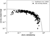 |
Fig. 1 BPT diagram of the selected nebular spectra. The dashed line represents the empirical relation by Kauffmann et al. (2003), which distinguishes between star-forming regions and AGNs. |
3 Nebular physical conditions and chemical abundances
3.1 Electron density and temperature
To determine the physical conditions of the gas, we use PyNeb 1.1.18 (Luridiana et al. 2015) with the atomic dataset presented in Table D1 and the H I effective recombination coefficients from Storey & Hummer (1995). We first employ the getCrossTemDen routine with line intensity ratios sensitive to ne and Te. We test density-sensitive diagnostics such as [S II] λ6731/λ6716, [O II] λ3726/λ3729, [Cl III] λ5538/λ5518, [Fe III] λ4658/λ4702, and [Ar IV]λ4740/λ4711 with temperature-sensitive diagnostics including [N II] λ5755/λ6584, [O III] λ4363/λ5007, [Ar III] λ5192/λ7135, and [S III] λ6312/λ9069.
First, each density-sensitive diagnostic is cross-correlated with all available temperature diagnostics using a Monte Carlo experiment of 100 points to propagate uncertainties in line intensities. For each convergence, a value of ne and Te and their associated uncertainties are obtained. The average ne, weighted by the inverse square of the error of the different convergences, is adopted as the representative value of the diagnostic (e.g., ne([O II] λ3726/λ3729)). This approach enables us to consider the small temperature dependence of density diagnostics under typical nebular conditions.
Once the density for each diagnostic is established, we follow the criteria suggested in Sect. 5 by Méndez-Delgado et al. (2023b) to estimate a global average density. If ne([S II] λ6731/λ6716) < 100 cm−3, we adopt ne = 100 ± 100 cm−3. If 100 cm−3 ≤ ne([S II] λ6731/λ6716) < 1000 cm−3, we adopt the average between ne([S II] λ6731/λ6716) and ne([O II] λ3726/λ3729). If ne([S II] λ6731/λ6716) ≥ 1000 cm−3, we adopt the averages of ne([S II] λ6731/λ6716), ne([O II] λ3726/λ3729), ne([Cl III] λ5538/λ5518), ne([Fe III] λ4658/λ4702), and ne([Ar IV] λ4740/λ4711). In cases where it is not possible to determine the density, such as in the spectra reported by Izotov et al. (2006), we adopt ne = 100 ± 100 cm−3.
Although there is temperature stratification (i.e., a representative temperature for each ionization volume, Stasińska 1978; Osterbrock & Ferland 2006; Peimbert et al. 2017; Berg et al. 2021), the possible existence of density stratification is not obvious among the different density diagnostics of H II regions (Méndez-Delgado et al. 2023b). These diagnostics have non-uniform sensitivities with ne, and are susceptible to systematic biases (Peimbert 1971; Rubin 1989; Tsamis et al. 2003; Méndez-Delgado et al. 2022a). The impact of these density biases is small in optical spectra if a good determination of Te is adopted (up to 0.1 dex if auroral lines are used to determine ionic abundances; Méndez-Delgado et al. 2023a; Rickards Vaught et al. 2024) but critical in chemical abundance studies with fine structure infrared CELs (Rubin 1989; Tsamis et al. 2003; Stasińska et al. 2013; Méndez-Delgado et al. 2024). Therefore, as a good approximation, adopting the global average density value, we estimate the temperatures Te([N II] λ5755/λ6584), Te([O III] λ4363/λ5007), Te([Ar III] λ5192/λ7135), and Te([S III] λ6312/λ9069) using the getTemDen routine from PyNeb.
Being a critical parameter, we exercise strict control over the determination of Te. In addition to excluding lines with errors larger than 40%, we compare the observed line intensity ratios of nebular transitions with their theoretical predictions. Lines arising from the same upper atomic level (e.g., [O III] λλ5007,4959, [S III] λλ9531,9069, [N II] λλ6584,6548) have fixed relative intensities given by the Einstein radiative coefficients, regardless of the physical conditions of the gas (Storey & Zeippen 2000). If the observed line intensity ratios differ by more than 20% from the theoretical predictions, their use for determining Te is discarded. In the particular case of [S III] λλ9531, 9069, when λ9531/λ9069 < 2.47, it is assumed that [S III] λ9531 is affected by telluric absorption bands (Noll et al. 2012), while [S III] λ9069 is not. This is the most common case in the literature with particular exceptions such as the Orion Nebula (Baldwin et al. 1996). Unfortunately, in a small number of cases, it is not possible to perform this test, as only one of the nebular lines is reported. In these cases, we consider the Te results valid. In any case, for this specific work, we only adopt T([S III]) to determine ionic abundances in the absence of T([N ii]) and T([O III]).
Another important case is that of Te([O III]), where [O III] λ4363 can be blended with [Fe II] λ4360 (Curti et al. 2017) when the spectral resolution is intermediate or low. In instances where we detected this blend, we discarded the use of [O III] λ4363, ensuring that we do not introduce spurious overestimations of Te([O III]). The impact of this blend is greater in regions of high metallicity and low ionization degree (Arellano-Córdova & Rodríguez 2020). Most of the star-forming regions with these characteristics analyzed in this work come from the CHAOS sample (Berg et al. 2015), which has taken special care in separating [O III] λ4363 and [Fe II] λ4360 (Berg et al. 2020; Rogers et al. 2021, 2022). Therefore, this potential observational issue will not systematically affect the analysis of the sample presented here. We show our derived physical conditions in Tables D3 and D4.
3.2 Ionic abundances
To determine the ionic abundances of Fe2+, N+, O+, and O2+, we use the [Fe III] λλ4658, 4702, [N II] λλ6548, 6584, [O II] λλ3727,3729, and [O III] λλ4959,5007 lines. In cases where both lines of each pair are available, we use the sum of their relative intensities to Hβ. Otherwise, we use the available line. In cases where [O II] λλ3727,3729 are not available due to spectral coverage limitations or observational defects in the blue arm, we use the auroral lines [O II] λλ7319,7320,7330,7331 to estimate the abundance of O+. Considering similarities in ioniza-tion potential, we adopt a common temperature, representative of low-ionization ions, to estimate the abundances of Fe2+, N+, and O+. In the same manner, to determine the abundance of O2+, we adopt a temperature representative of high-ionization.
Ionic abundances are estimated in two ways: considering a nebular homogeneous temperature structure (t2 = 0), known as “the direct method”, and accounting for the effect of an inhomogeneous temperature structure (t2 > 0) (Peimbert 1967). Following the empirical results of Méndez-Delgado et al. (2023a), we performed corrections for temperature inhomogeneities only for highly ionized ions. For t2 = 0, we adopt Te([N II] λ5755/ λ6584) and the global ne in the getIonAbundance routine of PyNeb, propagating uncertainties through 100-point Monte Carlo experiments. When Te([N II] λ5755/λ6584) is unavailable, we employ the temperature relations of Garnett (1992) to estimate Te([N II]) from Te([O III] λ4363/λ5007) or Te([S III] /λ6312/λ9069), when the first diagnostic is also absent. Similarly, the abundance of O2+ is determined using Te([O III] λ4363/λ5007) and the derived global average density. In cases where Te([O III] λ4363/λ5007) is not available, we use the temperature relations of Garnett (1992) along with measurements of Te([N II] λ5755/λ6584) and/or Te([S III] λ6312/λ9069). For t2 > 0, the treatment of low-ionization ions is identical to that described above. In the case of O2+, we adopt T0(O2+), estimated from Eq. (4) of Méndez-Delgado et al. (2023a). To roughly estimate the effect of t2 when Te([N II] λ5755/λ6584) is not available, we determine T0(O2+) by combining Eq. (4) of Méndez-Delgado et al. (2023a) with Eq. (2) of Garnett (1992).
In the present study, we do not add additional errors when using a temperature relationship to connect one Te diagnostic with another (e.g., if we have Te([N II]) with a 15% error, and we use a relationship to infer Te([O III]), we assume that Te([O III]) also has a 15% error). This is a lower limit to the uncertainties of the inferred temperature, similar to the approach of Skillman et al. (2003). However, we have been particularly careful about the impact of potential systematic errors introduced by the temperature relationships, with special emphasis on what happens in the low-metallicity regime. Under such conditions, the temperature relationships have not been sufficiently tested with empirical determinations, having limited statistics among simultaneous determinations of Te([N II]), Te([O III]), and T0(O2+) when Te > 13 000 K (Esteban et al. 2009; Berg et al. 2020; Arellano-Córdova et al. 2020; Méndez-Delgado et al. 2O23a,b). This is analyzed in greater detail in Appendix B. In general, the potential impact of severe systematic errors in the temperature relationships could be up to~0.05 dex in the Fe/O and Fe/N distributions. The adopted temperatures for determining the ionic abundances are shown in Table D5. Ionic abundances are shown in Table D6.
3.3 Total abundances
To estimate the total abundance of O/H, we directly sum the contributions of the ionic abundances O+/H+ and O2+/H+. The possible contribution of O3+/H+ was not considered, as it is expected to be very small (Amayo et al. 2021). In extremely metal-poor H II regions (12+log(O/H) < 7.5), ionization conditions may be harder than expected in photoionization models, leading to relatively strong emissions of He II. Under these conditions, an Ionization Correction Factor (ICF) can be implemented, as is typically done in the study of planetary nebulae (PNe, Torres-Peimbert & Peimbert 1977). However, observational studies on the contribution of O3+/H+ to the total O/H abundance in metal-poor regions often find values up to the order of 5% (Izotov & Thuan 1999; Domínguez-Guzmán et al. 2022). This was also found by Berg et al. (2021) in two Extreme Emission Line Galaxies with direct O3+/H+ abundances measured from the UV O IV] lines. This fraction is small for the purposes of this study and does not affect our conclusions. However, other studies such as those dedicated to estimating the He/O fractions must consider it, as they require a precision better than 1% (Peimbert & Torres-Peimbert 1974; Pagel et al. 1992; Izotov & Thuan 1998; Peimbert et al. 2002; Aver et al. 2015; Valerdi et al. 2019; Méndez-Delgado et al. 2020; Hsyu et al. 2020; Kurichin et al. 2021; Matsumoto et al. 2022).
The choice of t2 = 0 or t2 > 0 in determining the total O/H abundances of our observational sample of star-forming regions has an impact of 0.1–0.2 dex, as shown in Fig. 2. All determinations shown in black dots are based on CELs, following the procedure described in Sect. 3.2. For comparison, the figure displays abundances estimated with the temperature-insensitive O II RLs (red dots), in objects with the deepest spectra. Additionally, the solar reference by Asplund et al. (2021) is included. The choice of t2 = 0 or t2 > 0 results in differences of around 0.1–0.2 dex in the distributions of Fe/O and Fe/N, as discussed in Sect. 4. These differences may be relevant for the absolute values of Fe/O and Fe/N. On the other hand, the shape of the Fe/O and Fe/N distributions seems to remain unchanged, as it is shown in Appendix C.
From the entire sample, seven regions (Hubble V Peimbert et al. 2005, NGC 3603 García-Rojas et al. 2006, POX36, SBS0335-052E, J1205+4551 Izotov & Thuan 2004; Izotov et al. 2009, 2017, 2021, To11214-277 Guseva et al. 2011 and NGC 5449-2 Croxall et al. 2016) showed substantially higher O abundances in the case of t2 = 0 compared to the case t2 > 0 using the temperature relation proposed by Méndez-Delgado et al. (2023a). This suggests discrepancies between the values of Te([N II]) and Te([O III]) beyond temperature variations. The most obvious case is NGC 5449-2 (Croxall et al. 2016), where [N II] λ5755/λ6584 suggest a Te([N II])>40 000 K (see Table D4). This could be a non-reported observational error (Croxall et al. (2016) did not report Te([N II]) for this region, but they do not mention any observational problem that would necessitate discarding [N II] λ5755/λ6584). In the case of NGC 3603, it may be an aperture effect by not covering the entire Galactic nebula. Other regions like J1205+4551 could have over-estimations in Te([N II]) due to some phenomenon related to the presence of WR stars enriching the ISM with N (Izotov et al. 2021). In these cases, we adopt only the t2 = 0 values for our analysis, exerting no influence on our conclusions.
It is interesting to note that if t2 = 0 is considered in general, H II regions with abundances clearly higher than solar are rather rare, being only P203 and +30.8+139.0 from the M51 galaxy (Croxall et al. 2015), −35d7+119d6 from NGC 628 (Berg et al. 2015) and +75.7+89.1 and −35.7+119.6 from NGC 3184 (Berg et al. 2020), respectively. This, of course, could be a selection bias of our sample, dedicated to the detection of [Fe III] emission lines. However, in the literature, there are only ~20 additional examples of regions with Te -based metallicity estimations higher than solar (with t2 = 0) (Castellanos et al. 2002; Rosolowsky & Simon 2008; Bresolin et al. 2005; Bresolin 2007; Croxall et al. 2015, 2016; Lin et al. 2017; Patterson et al. 2012; Berg et al. 2015; Arellano-Córdova et al. 2021; Rogers et al. 2021, 2022). In our Galaxy, only Sh 2-48 and Sh 2-53 (Arellano-Córdova et al. 2021) would reach metallicities close to solar, but they are approximately 4 kpc closer to the Galactic center than the Sun. In contrast, massive O and B-type stars in the solar neighborhood (d < 3 kpc) typically exhibit solar or supersolar metallicities (Simón-Díaz et al. 2006; Nieva & Przybilla 2012; Martins et al. 2015; Weßmayer et al. 2022).
To determine the abundances of N/H and Fe/H, the use of an ICF is required to estimate the contributions of unobserved ionic states. In the case of N, it is necessary to estimate the contribution of N2+ in the ionized gas that does not emit lines in the optical spectrum. To this purpose, we adopt the scheme proposed by Amayo et al. (2021), based on photoionization models by Vale Asari et al. (2016) constructed using CLOUDY (Ferland et al. 2017). The ICF of Amayo et al. (2021) utilizes the similarity between the ionization potentials of N+ and O+ as proposed by Peimbert & Costero (1969), while also considering departures dependent on the ionization degree of the gas.
In the case of Fe, it is necessary to consider both the contribution of Fe+ and Fe3+. Although there are lines such as [Fe II] λ8617 or [Feiv] λ6740 optimal for the direct estimation of ionic abundances, these are generally very weak or found in complicated spectral regions affected by telluric absorptions. Therefore, initially one would think of using a classical ICF as those adopted in the case of other elements such as N, S, Ar, Ne (Amayo et al. 2021). Considering the ionization potentials of Fe2+, O+, and N+, the obvious choice would be to construct an ICF scheme considering the predictions of photoionization models on the relative abundances of these ions. However, Fe is a particularly complex element in star-forming nebulae because it is heavily depleted in dust grains. The relationships between the ionic fractions of Fe may be inconsistent with photoionization models if the fraction of Fe depleted in dust grains is different in the volumes where Fe+, Fe2+, and Fe3+ ions are located. We generally adopt the ICF proposed in Eq. (2) of Rodríguez & Rubin (2005). However, it is important to note that the Fe-ICF is a potentially important source of errors as is discussed in Sect. 4. ICF(N) and ICF(Fe) numerical values are presented in Table D7 while the total abundances are shown in Table D8.
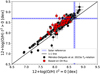 |
Fig. 2 Comparison of O/H abundances in the sample of star-forming regions considering a homogeneous temperature structure (t2 = 0) and considering temperature variations (t2 > 0) following the empirical relations derived by Méndez-Delgado et al. (2023a). Red dots indicate the O/H abundances determined from the ultrafaint O II-RLs, which are insensitive to temperature. The solar O/H abundance from Asplund et al. (2021) is shown for reference. |
4 The problematic calculation of the total gaseous Fe abundances in ionized nebulae
It is well known that different ICF schemes in the literature can yield significantly different results for various elements (e.g., see the discussions by Arellano-Córdova et al. 2020; Amayo et al. 2021; Arellano-Córdova et al. 2024). In the case of Fe, there is a systematic discrepancy between the predictions of Eq. (24) from Izotov et al. (2006) and Eq. (2) from Rodríguez & Rubin (2005). In Fig. 3, we show the comparison between both schemes in our sample of star-forming nebulae. The differences between these two ICFs for Fe can reach a systematic offset of up to ~0.2 dex (see also Kojima et al. 2021). To determine whether the ICF model of Izotov et al. (2006) overestimates the Fe abundances or the model of Rodríguez & Rubin (2005) underestimates them, or even the possibility that both models provide incorrect predictions, it is necessary to test both models in regions where direct estimates of all ionization states of Fe expected in the ionized gas are available.
In Table 1, we present the ionic and total abundances in a sample of nebulae with detections of [Fe IV] λ6740, which are useful for the direct estimation of Fe3+/H+ abundance. Other ionization states such as Fe+ and Fe4+ can be estimated using the lines [Fe II] λ8617, 8892 (Mendoza et al. 2023) and [Fe v] λ4227. To calculate the abundances of Fe+, we adopted the same temperature used to estimate the abundances of O+, N+, and Fe2+, while for the abundances of Fe3+ and Fe4+, we adopted the same temperature used for O2+ (see Sect. 3). We note that the contributions of Fe+ and Fe4+ to the total Fe abundances are generally very small, while the contribution of Fe3+ is always significant. The direct sum of ionic abundances can be compared directly with the predictions of Fe-ICFs by Rodríguez & Rubin (2005) and Izotov et al. (2006), which are based on the predictions of photoionization models using the measured abundance of Fe2+ and the degree of ionization. This exercise is performed for both t2 = 0 and t2 > 0. In this last case, the ionic abundances of Fe3+ and Fe4+ increase (Méndez-Delgado et al. 2023a), as well as the degree of ionization O2+/O+, which modifies the predictions of the Fe-ICF models.
As shown in Figs. 4 and 5, both Fe-ICFs exhibit a high dispersion compared to the directly determined values. Notably, the Fe-ICF by Izotov et al. (2006) overestimates the total Fe abundances in almost all cases, showing differences of up to ~0.7 dex compared to the directly estimated total value. Discrepancies between the predictions of photoionization models and the directly determined gaseous Fe values, considering t2 = 0, have been known since the pioneering work of Rubin et al. (1997). This discrepancy, known as “The [Fe IV] discrepancy” (Rodríguez & Rubin 2005), consists of photoionization models predicting Fe3+ abundances higher than those obtained observationally through the direct method, considering t2 = 0. This problem is clearly seen in the upper panels of Figs. 4 and 5, where practically all objects show higher Fe abundances in calculations using ICF. This issue appears to improve when considering the effects of temperature inhomogeneities, using the formalism of Peimbert (1967) and the empirical results of Méndez-Delgado et al. (2023a). Under this scheme, empirical abundances of highly ionized ions, such as Fe3+, increase when correcting the temperature bias introduced by an inhomogeneous physical conditions structure (Peimbert 1967; Cameron et al. 2023).
Although in the lower panel of Fig. 4, the data points lie both above and below the line (suggesting statistical rather than systematic errors), the dispersion remains very high at around ~0.2 dex. This dispersion may be due to various factors, including errors in the atomic models of Fe, as suggested by Rodríguez & Rubin (2005), or to the assumptions made to determine the ionic abundances. However, it is important to mention the possibility that such dispersion may be real, resulting from various physical phenomena. We suggest the possibility that the fraction of Fe trapped in dust may differ between the volume where Fe2+ and Fe3+ are present. It is expected that the energy of photons interacting with dust grains is different in the low and high ion-ization volumes, inducing a different dust grain fragmentation rate. Additionally, shock waves and stellar winds in the different ionization volumes may play a role. If the fraction of Fe trapped in dust grains is higher in the volume where Fe2+ coexists than where Fe3+ does, then an ICF based on the gaseous fraction of Fe2+ and the degree of ionization will underestimate the gaseous abundance of Fe, and vice versa. It is also possible that radiation pressure and stellar winds are capable of moving dust grains (Rodríguez 2002) from one ionization volume to another, inducing concentration variations in the nebulae.
Considering the present discussion, we adopt as default the ICF scheme from Eq. (2) of Rodríguez & Rubin (2005) and the nebular abundances considering t2 > 0. However, a greater number of nebulae with detections of the [Fe IV] λ6740 line or another transition of that ion would be highly beneficial for constraining potential errors in the total estimation of gaseous Fe in ionized nebulae.
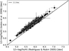 |
Fig. 3 Comparison between the Fe-ICF models of Izotov et al. (2006) and Rodríguez & Rubin (2005) in our adopted sample of star-forming nebulae. Both schemes were derived from photoionization models and are based on the determination of the ionic abundance of Fe2+. |
Ionic and total Fe abundances compared to the predictions of the Fe-ICFs from Rodríguez & Rubin (2005) and Izotov et al. (2006), which are derived from photoionization models.
5 Gas phase Fe distributions
5.1 Fe and O nebular abundances
In Fig. 6, we present the distribution of Fe/O, both in Galactic stellar objects and in Galactic and extragalactic star-forming nebulae. In the stellar panel, the observed distribution is well-known (Amarsi et al. 2019; Kobayashi et al. 2020; Chruślińska et al. 2024) and exhibits an increasing trend with respect to O/H. This is consistent with the predictions from the different enrichment timescales of CCSNe as primary O producers and SNe-Ia as primary Fe producers (e.g., Chruślińska et al. 2024). It is important to note that at the low metallicities covered in our sample, Fe/O remains relatively constant, with log(Fe/O)=-1.80 ± 0.11, consistent with the value reported by Amarsi et al. (2019) and Chruślińska et al. (2024) for Galactic low-metallicity dwarf stars. The stellar distribution of Fe/O vs O/H resembles the distribution of N/O versus O/H observed in nebular regions (Henry et al. 2000; Nava et al. 2006; Nicholls et al. 2017). These analogous behaviors can be explained by the similar timescales required to form a white dwarf in a stellar system that gives rise to a SN-Ia (Fe producers) and that required for an intermediate-mass star to release the N produced via CNO processes (~40 Myr).
Although there is a relatively small number of objects (23, see Table 2) with 12+log(O/H)<7.6, most of the star-forming nebulae in the lower panel of Fig. 6 seem to exhibit a flattening in the Fe/O distribution around log(Fe/O)=−1.74 ± 0.15, rather consistent within the errors with the log(Fe/O)=−1.80 ± 0.11 determined in stellar objects. This may indicate that regions within this range of O/H abundances exhibit a negligible fraction of Fe depleted in dust. Under these conditions, the gaseous abundance of Fe would be representative of the total abundance of this element in ionized nebulae.
In the lower panel of Fig. 6, as the O/H abundance increases beyond 12+log(O/H)≈7.6, Fe/O rapidly decreases, in contrast to the behavior observed in stellar objects. This trend is the result of Fe depletion onto dust grains within the ionized nebulae (Rodríguez 2002; Rodríguez & Rubin 2005; Izotov et al. 2006; Izotov et al. 2021). The fraction of Fe trapped in dust grains increases with metallicity mainly due to two factors. First, as metallicity increases, the ionizing sources in the nebulae tend to be softer (Vilchez & Pagel 1988; Stasińska et al. 2015). This makes it less likely for dust grains in the ionized gas to shatter upon being hit by energetic photons (Rodríguez 2002). Second, the formation of solid Fe compounds is proportional to the availability of this element. As seen in the upper panel of Fig. 6, the abundance of Fe/H increases more rapidly than O/H at high metallicities.
Although the decreasing trend of Fe/O at high values of O/H is clear, the dispersion is relatively high (~0.3 dex) and the Pearson correlation coefficient is only moderate (r = −0.59). Based on Sloan Digital Sky Survey (SDSS) spectra (Abazajian et al. 2005), Izotov et al. (2006) have suggested that the high dispersion in the Fe/O relation may be dominated by the errors in the flux measurements of the faint [Fe III] lines. In Fig. 7, we consider the subsample of our nebular regions with the deepest spectra, with uncertainties in the [Fe III] λ4658 intensity below 10%. This figure shows a correlation coefficient practically identical to that found in the general sample of nebulae and a relatively high dispersion, suggesting that much of the dispersion is real and caused by a physical reason as those mentioned in Sect. 4.
An important factor that may contribute to the scatter is the presence and propagation of shocks in the nebular gas (Rodríguez 2002). Several studies (Blagrave et al. 2006; Mesa-Delgado et al. 2009; Espíritu et al. 2017; Méndez-Delgado et al. 2022b) have observationally demonstrated the ability of photoionized shocks to break dust grains and release Fe into its gaseous phase. However, we propose that the relationship between Fe/O and O/H does not exhibit a higher linear correlation simply because the phenomena inducing Fe depletion in dust grains are not perfectly linearly related to the abundance of O/H. Although there is a relationship between the radiation hardness and the abundance of O/H, it is not linear (Morisset 2004; Simón-Díaz & Stasinska 2008). In contrast, the effective temperature of the ionizing stars and the importance of their stellar winds depends primarily on Fe rather than O (Garcia et al. 2014; Chruślińska et al. 2024). More importantly, the total abundance of Fe, on which the formation of Fe-rich dust compounds could depends, does not scale linearly with that of O at high metallicity, as shown in the upper panel of Fig. 6.
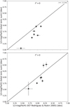 |
Fig. 4 Comparison between the Fe abundances obtained directly from the sum of the ionic abundances present in the gas in the sample of regions of Table 1 and those determined using the Fe-ICF of Rodríguez & Rubin (2005) derived from photoionization models. Upper panel: chemical abundances calculated considering a homogeneous nebular temperature structure (t2 = 0). Lower panel: chemical abundances calculated considering the presence of temperature inhomogeneities (t2 > 0). |
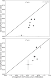 |
Fig. 5 Analogous to Fig. 4 but considering the Fe-ICF scheme of Izotov et al. (2006). |
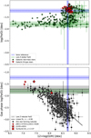 |
Fig. 6 Distribution of log(Fe/O) vs 12+log(O/H). Upper panel: Milky Way stars from the sample described in Sect. 2. Lower panel: galactic and extragalactic star-forming nebulae. The red dots highlight the positions of J0811+4730 (Izotov et al. 2018) and J1631+4426 Kojima et al. (2021), recently interpreted by Kojima et al. (2021) as enriched in Fe. The red stars indicate the position of J1205+4551 (Izotov et al. 2017, 2021), a galaxy with elevated Fe/O abundances and evidence of WR activity. The red cross points out the location of the Sunburst Arc (Welch et al. 2024), a high-redshift (z = 2.37) galaxy recently observed by the JWST. Nebular O/H estimates consider the influence of nebular temperature variations (t2 > 0). The solar Fe/O and O/H abundances from Asplund et al. (2021) are shown as a reference. r is the Pearson correlation coefficient of the linear fit. |
5.2 Fe and N nebular abundances
Considering the hypothesis that the timescale to form a white dwarf in a stellar system that produces a SN-Ia is similar to the timescale over which an intermediate mass star returns secondary N to the ISM, we decided to explore the Fe/N distribution. If this hypothesis holds true, then the production of Fe at high metallicities should be better correlated with that of N rather than O. In Fig. 8, we present the distribution of log(Fe/N) as a function of 12+log(N/H) both in Milky Way stars (upper panel) and in star-forming nebulae (lower panel), analogous to what is presented in Fig. 6.
Despite the significant dispersion in the upper pannel of Fig. 8, the observed Fe/N ratio in low-mass stars can mostly be encompassed around a relatively flat band, represented by a green dashed line in Fig. 8 and which corresponding parameters are given in Table 2. This trend can be explained by the findings of different studies where the stellar abundance of Fe scales linearly with that of N even in wider abundance ranges than those considered in this work (Israelian et al. 2004; Ecuvillon et al. 2004; Magrini et al. 2018; Kobayashi et al. 2020; Grisoni et al. 2021). Notably, when examining the B-type stars studied by Nieva & Przybilla (2012) and Weßmayer et al. (2022), shown in red triangles in the upper pannel of Fig. 8, a strongly linear Fe/N correlation is observed, contrasting with the Fe/O relationship observed in this same stellar sample. These stars have formed more recently than the lower-mass star sample and have been enriched with metals. It is likely that the N present in these B-type stars in the solar neighborhood has been modified via the CNO cycle and mixing processes (Przybilla et al. 2010). In such case, these stellar N abundances would not be comparable to those of H II regions or other stellar systems. On the other hand, the Fe/H abundance shows little variation, suggesting homogeneous production of Fe/H in the interstellar medium that contributed to the formation of these B stars. This will be further discussed in Sect. 6.4.
In the lower panel of Fig. 8, we show the distribution of gaseous Fe/N in star-forming nebulae, similar to that shown in the lower panel of Fig. 6 for Fe/O. The higher Pearson correlation coefficient suggests that the linear correlation between Fe/N abundance and N/H is stronger than that observed for Fe/O and O/H, althought the dispersion remains quite high ~0.3 dex, similar to what is found in the Fe/O vs O/H distribution. This could indicate that some of the key factors in the Fe dust depletion have a closer relationship with N abundance than with O. Given the close relationship between the stellar abundances of Fe and N observed in the upper panel of Fig. 8, it seems plausible that the nucleosynthetic production of Fe is better correlated with that of N, due to similarities in the timescales required for SN-Ia production and the evolution of intermediate-mass stars. The use of N as a proxy for Fe would allow us to capture the systematic effect of radiation hardness, which is capable of destroying dust grains in photoionized environments (Rodríguez 2002) and scales with the abundance of Fe/H (Garcia et al. 2014; Chruślińska et al. 2024). Additionally, N exhibits insignificant depletions even in neutral environments of high metallicities (Jenkins 2009).
Similarly to what is presented in Fig. 7 for the Fe/O vs O/H distribution, in Fig. 9 we show the Fe/N vs N/H distribution considering only the regions where [Fe III] λ4658 has uncertainties in its intensity lower than 10%. This figure shows that the general distribution observed in Fig. 8 is maintained, although with less dispersion. Additionally, an apparent flattening in the distribution is observed when 12+log(N/H) < 6.3. This flattening is not observed in the general sample and will be discussed in more detail in Sect. 6.
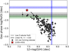 |
Fig. 7 Same as the lower panel of Fig. 6 but considering only regions with errors in the [Fe III] λ4658 line intensity of smaller than 10%. |
6 Discussion
6.1 Possible empirical relations for dust depletion
As shown in Fig. 6 when 12+log(O/H) < 7.6 the nebular gas-phase Fe/O seems to reach a constant value, or at least change the slope of the general trend, being consistent with the abundance one observed in Galactic stars in the same metallicity range. This flattening may suggests that the fraction of Fe trapped into dust in these photoionized nebulae is very small. This could be explained by the fact that the photoionization conditions in metal-poor regions are harder (Vilchez & Pagel 1988; Stasińska et al. 2015), making the destruction of dust grains more efficient. At the same time, the availability of Fe, essential for the formation of some solid compounds, is very low. Determining the metallicity ranges where total Fe can be directly inferred from gaseous Fe is very important because it could point out to significant differences in the impact of dust in local ionized environments (generally of higher metallicity) and those observed in less evolved galaxies, such as those currently detected with the JWST. This could also help to explain why some Fe lines have been detected in high-z galaxies (Arellano-Córdova et al. 2022; Ji et al. 2024; Tacchella et al. 2024; Welch et al. 2024), despite being very weak in local H II regions.
However, the flattening effect is not clearly seen in the general distribution of Fe/N presented in Fi.g 8. This is a bit puzzling as it seems well established that nebular N/O abundance reaches a plateau at low metallicities (Garnett 1990; Nava et al. 2006; Skillman et al. 2013; Nicholls et al. 2017) and therefore, one would also expect to observe a flattening in Fe/N if it is present in Fe/O. In our sample, the regions 0556-51991-31, J0811+4730, and SBS-0335-052E (Izotov et al. 2006; Izotov et al. 2009, 2018) seem to extend the linear trend between Fe/N and N/H observed at high metallicities. This could be a consequence of the changes in the gaseous abundance of Fe due to different depletion patterns being small and going unnoticed when compared to the abundance of O, as it is an element much more abundant than N. Alternatively, this could simply be a problem of low statistics when 12+log(N/H) < 6.5. In fact, such flattening seems to begin to appear in Fig. 9, which shows the Fe/N distribution only in regions with the best signal-to-noise ratio in [Fe III] λ4658. Notably, in low metallicity regions, the detection of [N II] λλ6548, 6584 is more challenging than in the case of [Fe III] λ4658. In fact, in this work, we have more regions with direct determinations of Fe and O than that of Fe and N. In our DESIRED sample, using the same criteria described in Sect. 3, we determine that when 12+log(O/H) < 8.0, log(N/O) ~ −1.3 (Arellano-Córdova et al. in prep.). Therefore, we adopt 12+log(N/H) = 6.3 as equivalent to 12+log(O/H) = 7.6. However, we find a relatively high dispersion (~0.3 dex) around this value.
If we assume that the total abundance of Fe scales in proportion to that of N, as suggested by stellar abundances and the previous discussion, it is possible to determine an empirical relationship to approximately determine the fraction of Fe trapped in dust as a function of the N/H abundance. In Eq. (1), we present this relation considering only the nebular values given in Table 2. Eq. (1) is valid for high-metallicity nebulae, where 12+log(O/H) ≥ 7.6 or 12+log(N/H) ≥ 6.3. For values lower than these, FeDust/FeTotal ≈ 0.
 (1)
(1)
Equation (1) implies that the formation of Fe-rich dust grains grows predominantly in proportion to the same Fe abundance. From this equation, the proportionality factor (1 × 10⁻⁵) presents the greatest uncertainties as it is mainly based on the Fe/N nebular values when 12+log(N/H) < 6.3. In contrast, the power (−0.91) is much more robust as it represents the slope of the relationship between Fe/N and N/H considering 382 objects with 12+log(N/H) > 6.3. Considering a solar N abundance of 12+log(N/H) = 7.83 (Asplund et al. 2021), Eq. (1) indicates that approximately ~95% of the Fe in ionized nebulae is depleted into dust grains. On the other hand, considering the values of the Large Magellanic Cloud (LMC) and the Small Magellanic Cloud (SMC; 12+log(N/H)=7.1–7.2 and 12+log(N/H)=6.5–.7, respectively, see Table D8), the fractions would be approximately ~75% and ~35%, respectively. In the case of the SMC, the nitrogen abundance values are at the limit of validity of Eq. (1). The fraction of ~35% assumes a value of 12+log(N/H)=6.7, but a negligible O-dust fraction of ~1% is expected if 12+log(N/H)=6.5 is considered. In Fig. 10, we show the total Fe/O abundance in the entire sample of star-forming nebulae, considering the gaseous fraction of Fe/H, measured from the [Fe III] emission, and the fraction of Fe/H depleted into dust, inferred from Eq. (1). There is a rather good consistency between the stellar and nebular abundance distributions, as indicated by the binned values marked with red stars and black dots.
Typically, the Fe/O versus O/H relationship (or more commonly [O/Fe] vs. [Fe/H]1) is used to understand the star formation history of a particular galaxy (Kobayashi et al. 2006; Magrini et al. 2010; Matteucci 2012). In this relationship, star formation efficiency and the Initial Mass Function are parameters that play a fundamental role. Similarly, these same parameters govern the N/O vs. O/H relationship (Mollá et al. 2006). Considering a large number of star-forming regions from different galaxies, it is well established observationally that the N/O vs. O/H relationship reaches a plateau at low metallicities (12+log(O/H) < 8) (Henry et al. 2000; Nava et al. 2006; Nicholls et al. 2017) determined by the onset of N production from intermediate mass stars (Vincenzo et al. 2016). If there is a close relationship between the production times of Fe and N, one would also expect a plateau in the Fe/O vs. O/H relationship among various star-forming regions, once the fraction of Fe trapped in dust grains has been considered. By looking at the binned nebular values in Fig. 10 we indeed observe a plateau up to roughly 12+log(O/H) = 8.0, with a subsequent rise in the Fe/O ratio. Moreover, the position of this “knee”, which indicates the onset of SNe Ia contribution, also agrees with the one observed in Galactic stars considered in this work. In turn, this means that, on average, star-forming regions in present-day local galaxies share a similar level of efficiency of star formation and Initial Mass Function shape relative to the one already experienced by the Galactic disk, capturing different evolutionary snapshots according to their metallicity. This appears to be at odds with stellar abundances observed in dwarf galaxies of the Local Group. For example, dwarf spheroidal galaxies show an O/Fe plateau (deduced from other α-elements) roughly from 12+log(O/H) < 7.5 (Hendricks et al. 2014; Hill et al. 2019). However, these galaxies are faint, gas-poor, and quiescent in star formation (see e.g., Tolstoy et al. 2009). This indicates that nebular observations of galaxies with low O/H abundance will be biased toward regions of intense star formation corresponding to gas-rich, dwarf irregular galaxies. The position of the O/Fe plateau in irregular dwarf galaxies is still relatively uncertain, as there are very few determinations beyond local systems as the SMC and LMC, which might differ from the conditions of other lower-metallicity systems with a higher star formation rate.
Nonetheless, the position of the “knee” could still show differences relative to the mean trend due to the different evolutionary history in each galaxy. This causes the significant dispersion in the nebular abundances in Fig. 10, in addition to other factors contributing to the uncertainties in Fe, dominated by the correction for depletion onto dust grains. In fact, the distribution presented here in Fig. 10 is valid if the possible O/Fe plateau occurs when 12+log(O/H) < 7.6. The precise position of the expected O/Fe-plateau may induce offsets in the nebular distribution of Fe/O observed, but in general, the functional form would not be altered.
Figure 10 also reinforces the fact that the conversion between stellar metallicities, measured with Fe, and nebular metallicities, measured with O, is not straightforward. Significant biases can be expected when transforming individual stellar Fe abundances to O abundances using the solar reference as in Bresolin et al. (2009, 2016, 2022). In the best case scenario, when indeed we are within the range of solar metallicities, both stars and nebulae exhibit average dispersions of up to ~0.2 dex in the Fe/O abundances, resulting from production variations between Fe and O. We think it is important to consider this uncertainty when comparing stellar and nebular metallicities. A much worse situation arises when comparing stellar and nebular galactic abundance gradients using the solar reference of Fe/O as a conversion factor as used in several works (e.g. Gazak et al. 2015; Bresolin et al. 2022), as the entire abundance pattern changes with metallicity. Using the stellar reference of Fe/N that we present in Table 2 could be potentially useful in this latter case. However, a larger statistical sample for stellar Fe and N abundances is required for this purpose. An alternative based on the knowledge of the specific SFR of the system is presented by Chruślińska et al. (2024).
As suggested by Peimbert & Peimbert (2010), in the case that the depletion of O onto dust grains scales with that of Fe, it is possible to derive an upper limit to the O depletion. In the case of the Orion Nebula, it is known that the fraction of dust trapping O is up to ~0.1 dex (Mesa-Delgado et al. 2009; Peimbert & Peimbert 2010). Therefore, it can be estimated that in the LMC and SMC there may be up to ~0.07 dex and ~0.03 dex of O trapped in dust, respectively. The depletion of O onto dust could be negligible at 12+log(O/H) < 8.0, as its contribution is much smaller than the typical uncertainties in the estimation of chemical abundances in ionized nebulae. We remark that these could be considered upper limits to the depletion of O in photoionized environments as they are based on a scaling of the upper limit derived for the Orion Nebula. Therefore, simply adding 0.1 dex to correct for dust all nebular determinations of O/H, regardless of metallicity and ionization conditions – as it has been done in several works (e.g., Bresolin et al. 2016, 2022) – seems inappropriate.
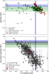 |
Fig. 8 Distribution of log(Fe/N) vs 12+log(N/H). Upper panel: Milky Way stars from the sample described in Sect. 2. Lower panel: Galactic and extragalactic star-forming nebulae. The red dot highlights the position of J0811+4730 (Izotov et al. 2018), recently interpreted by Kojima et al. (2021) as enriched in Fe. The red star indicates the position of J1205+4551 (Izotov et al. 2017, 2021), a galaxy with elevated Fe/O abundances and evidence of WR activity. The red cross points out the location of the Sunburst Arc (Welch et al. 2024), a high-redshift (z = 2.37) galaxy recently observed by the JWST. Nebular N/H estimates consider the influence of nebular temperature variations (t2 > 0). The solar Fe/N and N/H abundances from Asplund et al. (2021) are shown for reference. r is the Pearson correlation coefficient of the linear fit. |
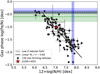 |
Fig. 9 Same as the lower panel of Fig. 8 but considering only regions with errors in the [Fe III] λ4658 line intensity smaller than 10%. |
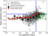 |
Fig. 10 Total Fe/O vs. O/H abundance ratios for Galactic stars (green stars) and gas-phase abundance ratios for star-forming nebulae (gray circles). The plotted gas-phase abundances include the contribution from the dust-depleted Fe fraction calculated using Eq. (1). The binned values (with bins of 0.2 dex) appear as red stars and black circles for Galactic stars and star-forming nebulae, respectively. |
6.2 Dust composition in H II regions
The precise chemical composition of dust in ionized gas remains a matter of debate (Simón-Díaz & Stasińska 2011), and its impact on the important parameters of ionized nebulae could be significant (Gunasekera et al. 2023). The dust present in H II regions should consist of the grains most resistant to photoionization, formed prior to star formation. This is supported by the fact that we do not observe any connection between the depleted Fe fraction and the electron density, a case that could be expected if a significant fraction of the dust grains were formed within the photoionized environment (Zhukovska et al. 2018). In our Appendix A, we show a weak anticorrelation between optical reddening relative to Hβ and the Fe/O and Fe/N abundances in a subsample of the regions analyzed in this work. The anti-correlation seems stronger in the case of Fe/N. This reinforces the idea of having an interconnection between the dust found in H II regions and that present in the neutral medium, which may cause most of the optical extinction. Studies of dust in the neutral ISM can provide candidates that may survive photoionization and be present in H II regions. In situ studies of dust in the neutral ISM indicate that it is likely that Fe is mostly locked up in free-flying iron particles and silicate grains (Jones et al. 2017; Choban et al. 2022; Hensley & Draine 2023; Dubois et al. 2024).
Our results from Figs. 6 and 8 show that the fraction of Fe trapped in dust grains decreases as metallicity decreases. Our interpretation is that photo-destruction is particularly important at lower metallicities (Rodríguez 2002; Rodríguez & Rubin 2005) because the ionizing spectrum becomes increasingly harder as the amount of Fe in stars decreases (Vilchez & Pagel 1988; Stasińska et al. 2015). In turn, the gas-to-dust fraction in the neutral ISM tends to be higher at lower metallicities (Gioannini et al. 2017; Galliano et al. 2021; Roman-Duval et al. 2022b,a), which suggests that there is less Fe-rich dust in low-metallicity ionized environments because the fraction of Fe trapped in dust in the neutral ISM is lower prior the star formation. In fact, the relation we find between Fe/O and O/H is similar to the relation found by Gioannini et al. (2017) between Fe/Zn vs. Zn/H and Fe/S vs. S/H in neutral gas. Both the increased photo-destruction of dust grains in low-metallicity ionized environments and the reduced formation of dust in the low-metallicity neutral ISM are not mutually exclusive and could be acting in the same direction. It is important to mention that spatially resolved studies of the distribution of gaseous Fe/H in H II regions of our Galaxy, as is possible with the SDSS-V Local Volume Mapper (Drory et al. 2024), are of great importance to quantify the impact of dust photo-destruction in ionized environments. Preliminary results from the Orion Nebula (Méndez-Delgado et al. in prep.) show an increasing trend of Fe/O and Fe/N when approaching the ionizing star θ1 Ori C, suggesting that the impact could be significant.
Photo-destruction should mainly affect the smaller grains, particularly the carbonaceous ones (Jones et al. 2017). Studies of photoionized Herbig-Haro objects in the Orion Nebula (Blagrave et al. 2006; Mesa-Delgado et al. 2009; Méndez-Delgado et al. 2021a; Méndez-Delgado et al. 2021b, 2022b) show dramatic increases in the gaseous abundances of Fe, Ni and Cr at the bowshocks due to the destruction of dust present in the photoionized gas. In contrast, in these objects, the abundances of O and C remain virtually unchanged. This suggests that most of the Fe depleted in grains could be composed of Fe grains decoupled from C and O that could be efficiently destroyed by the ionizing radiation. This could suggest that most of the Fe-dust in ionized environments is composed by free-flying iron particles.
Interestingly, the fact that we find a significant depletion of Fe in dust grains in a large number of objects indicates that these grains were not yet processed by the supernova forward shock, which is predicted to destroy a large fraction of the dust grains (Bocchio et al. 2014; Slavin et al. 2015; Kirchschlager et al. 2022, 2024). However, given the large dispersion observed in the distributions of Fe/N and Fe/O, it cannot be ruled out that supernova shocks are playing a role in some fraction of the regions analyzed here.
6.3 Fe enrichment by very massive stars on short timescales
Recently, Kojima et al. (2021) reported a puzzlingly high Fe/O in J0811+4730 and J1631+4426, two of the extremely metal-poor local dwarf galaxies in their sample. Such an abundance pattern cannot be explained by enrichment from regular CCSNe, and the inferred young age and very high specific SFR in those galaxies rule out the possibility of significant Fe enrichment by SNe Ia. Kojima et al. (2021) speculate that the high Fe/O could be indicative of enrichment by very massive stars with Minit > 300 M⊙. Other scenarios, involving enrichment by massive pair-instability supernovae and a non-universal IMF, have also been proposed Goswami et al. (2021).
Our results presented in Sect. 4 suggest that Kojima et al. (2021) overestimate the Fe abundances in J0811+4730 and J1631+4426 due to the bias introduced by the Fe-ICF they use (that proposed by Izotov et al. 2006). We argue that these abundances are overestimated by at least ~0.2 dex. However, we point out that the adoption of the ICF by Izotov et al. (2006) can introduce overestimations of the Fe abundances of up to ~0.7 dex in environments where the Fe3+/Fe fraction is higher, which are precisely metal-poor regions like J0811+4730 and J1631+4426 (Rodríguez & Rubin 2005).
Additionally, in contrast with the discussion presented by Kojima et al. (2021), we show that the trends observed in Figs. 6 and 8 can be explained in terms of the depletion of Fe onto dust grains in ionized environments. The existence of such dust is firmly established by various studies of local nebulae (Rodríguez 1999, 2002; Rodríguez & Rubin 2005; Blagrave et al. 2006; Mesa-Delgado et al. 2009; Méndez-Delgado et al. 2021a) that include direct detections of the dust emissions (Smith et al. 2005). On the other hand, Kojima et al. (2021) did not find any correlation between the dust extinction and the Fe/O ratios. However, although local dust trapping Fe in Galactic nebulae could have some effects on the observed optical extinction due to their proximity to us (Rodríguez 2002), this effect may be negligible in more distant systems where the influence of dust outside the H II region and integrated along the line of sight could play the most significant role.
Although J0811+4730 and J1631+4426 certainly exhibit a slightly elevated Fe/O abundance, they remain basically consistent with values obtained in other regions with low O/H abundances, explained in terms of preferential dust depletion. Therefore, we do not find compelling evidence of Fe overproduction by stars with Minit > 300 M⊙ in these objects.
Interestingly, in the lower panel of Fig. 6 two spectra of J1205+4551 highlighted by the red stars (Izotov et al. 2017, 2021), show Fe/O abundances similar to those found by Kojima et al. (2021) in J0811+4730 and J1631+4426. J1205+4551 additionally exhibits signatures of WR stars (Izotov et al. 2021) and a very high N/O abundance for its O/H abundance. In more massive stars, surface nitrogen quickly gets enriched at the expense of oxygen. Strong stellar winds can then lead to an enrichment of the ISM with nitrogen (Meynet & Maeder 2005; Crowther 2007; López-Sánchez et al. 2007). In particular the WN stage can provide an efficient channel here as the products of He burning have not yet reached the stellar surface, but the winds are stronger than for normal O stars. This effect is prominently seen in the abundances of resolved nebulae around massive WN stars (e.g., Kwitter 1984; Stock et al. 2011; Esteban et al. 2016), and consequently predicted for the yields of very massive, hydro-burning stars (Minit ≥ 100 M⊙) that also show WNh-type spectra (e.g., Higgins et al. 2023). The effect of WR stars on Fe is not entirely clear, mainly due to the high depletion of this element onto dust grains at high metallicities.
In contrast to the Fe/O abundance, as shown in Fig. 8, the Fe/N abundance in J1205+4551 does not appear anomalous, but rather consistent with the general trend. Another interesting case is the Sunburst Arc, a galaxy at z = 2.37 recently observed with the JWST and analyzed by Welch et al. (2024). This latter galaxy presents a high N/O abundance, unexpected for its low O/H abundance. However, in Fig. 8, we find that, similarly to the case of J1205+4551, the Sunburst Arc (highlighted by the red cross) shows quite a normal Fe/N abundance. This might indicate that some nebular regions with abnormally high N/O abundances could also contain rather high Fe/O abundances. It is possible to speculate that the high values of Fe/O and N/O in these regions may be due to a lower availability of O resulting from the presence of WR stars. A systematic study of the Fe/H abundance in H II regions with low O/H abundances and high N/O ratios like some particular knots of NGC 5471 (Kennicutt et al. 2003) or Mrk 71 (Esteban et al. 2002), may shed light on this interesting issue.
6.4 Stellar and nebular metallicities
The main idea to interpret the linear relation between gas-phase abundances of Fe and N in star-forming nebulae is that the production timescales of N and Fe are similar, while dust formation trapping Fe scales with its own availability. This seems valid in the range of chemical abundances studied here (Magrini et al. 2018; Xiong et al. 2022; Sun et al. 2023), and is consistent with the assumption of the primary origin of N in CCSNe of massive stars and secondary in intermediate-mass stars through the CNO cycle (Henry et al. 2000; Meynet & Maeder 2002b,a). In general, the different nucleosynthetic origins of N and Fe can add additional complexity to the empirical abundances of both elements. For instance, N enrichment from intermediate-mass stars is known to be sensitive to metallicity (Ventura et al. 2013). Such metallicity-sensitive yields could decouple the gas-phase Fe and N abundances, specially at supersolar metallicities. Nevertheless, within the metallicity range covered by this analysis, which encompasses most of the nebular analyses reported in the literature, such deviations are not observed. The yield predictions from Ventura et al. (2013) appear consistent with observational stellar values within the analyzed metallicity range, as illustrated in Fig. 1 of Romano et al. (2019) (corresponding to models MWG06 and MWG07). Our study does not extend beyond the metallicity ranges discussed in these works. Future studies that cover metallicity ranges beyond those examined here could investigate these predictions.
Some authors have suggested the existence of massive stars with high rotation velocities as a source of N observed at low metallicities (Limongi & Chieffi 2018; Prantzos et al. 2018), being able to successfully reproduce the observed flat trends between Fe/N and N/H in Galactic stars (Prantzos et al. 2018; Limongi & Chieffi 2018; Romano et al. 2019). These differences in the precise origin of N at low metallicities do not seem to affect our interpretation, at least within the range of our chemical determinations, as the production timescales remain similar.
As observed in the upper panel of Fig. 8, Galactic B-type stars (Nieva & Przybilla 2012; Weßmayer et al. 2022) show more significant variations in the Fe/N ratio compared to the other stars analyzed here. This trend is not limited to Galactic B-type stars but is also evident in other galaxies (Trundle & Lennon 2005; Trundle et al. 2007; Evans et al. 2007; Hunter et al. 2007). For instance, in the SMC, LMC, and NGC 3109, massive B-type stars (both giants and dwarfs) analyzed by Hunter et al. (2007) and Evans et al. (2007) typically exhibit nitrogen overabundances of more than one order of magnitude compared to nebular values (Peña et al. 2007; Toribio San Cipriano et al. 2017; Domínguez-Guzmán et al. 2022), reflecting that massive stars rapidly reach the so-called “CN” equilibrium as a part of the CNO cycle (Przybilla et al. 2010). Confirmed by recent efforts of the XShootU collaboration (Martins et al. 2024), it seems that in galaxies with lower overall O/H abundance, massive stars exhibit higher N/H overabundances. However, determining whether this is systematic or merely a selection bias towards the brightest stars in these systems goes beyond the scope of this study. Nevertheless, it is important to note that N/Fe and N/O ratios in these stars do not constitute the final value that will be released into the ISM after their death in CCSN.
Interestingly, the very high overabundances of N observed in some extragalactic B-type stars could significantly alter the abundances of C and O. If a significant portion of the N is produced at the expense of O, non-negligible decrements, on the order of ~0.1−0.2 dex, may be present (Martins et al. 2024). This complicates element-by-element comparisons between the abundances of C, N, and O among massive B-type stars and H II regions when high precision is required. Studies of individual, unevolved OB stars which do not exhibit significant mixing processes (e.g., Rolleston et al. 2003; Ramachandran et al. 2021; Pauli et al. 2023; Martins et al. 2024) could provide a very useful testbed for the consistency between present-day stellar and nebular abundances. Yet, if achieving high precision in the comparisons between O abundances in stars and nebulae is already complicated, it becomes even more so when dealing with stellar metallicities derived from the analysis of combined absorption lines of various elements (but dominated by Fe-peak elements, Urbaneja et al. 2008; U et al. 2009; Kudritzki et al. 2008, 2012, 2014, 2016; Hosek et al. 2014; Patrick et al. 2015), as done by Bresolin et al. (2016) in several galactic systems using the solar reference to transform Fe-metallicities into O-metallicities. Direct O measurements instead are typically focussed on very slow rotating stars such as the prototypical B-type dwarf AzV 304 (Rolleston et al. 2003). While such stars allow for a high-precision O measurement due to the narrow lines, this limited selection might imply a bias in itself.
We are aware that the number of star-forming nebulae with 12+log(O/H) < 7.6 in our sample is somewhat limited, but it already constitutes a significant observational achievement to have direct nebular determinations of Fe, O, and N under such conditions. The change in the slope of the Fe/O abundance ratio in this range of metallicities could be very small. If the value of log(Fe/O) ~−1.74 is representative of the total Fe/O abundances in these star-forming nebulae in the metallicity range –which correspond to dwarf irregular galaxies– this could indicate similar star formation efficiencies than what was present, in the early stages of the Milky Way (Carigi et al. 2005, 2019; Nomoto et al. 2013; Amarsi et al. 2019; Kobayashi et al. 2006, 2020; Prantzos et al. 2023). In contrast, if new observations of star-forming nebulae were to show a continuation of the anti-correlation between Fe/O and O/H produced by Fe depletion in dust grains, this could indicate lower star formation efficiencies or the presence of some phenomenon such as metal losses through winds (Tolstoy et al. 2009).
A high Fe/O ratio in low O/H environments would imply harder thermal equilibrium in ionized nebulae than what is typically observed in local H II regions. On the one hand, the stellar winds from ionizing stars are more significant as a function of the Fe abundance (e.g., Vink et al. 2001; Garcia et al. 2014; Sander et al. 2020; Chruślińska et al. 2024). On the other hand, gas cooling is mainly driven by the O abundance (Osterbrock & Ferland 2006). However, a potentially high rate of Fe production through SN-Ia events should occur on timescales similar to those of secondary N production in intermediate-mass stars, and it seems well established that in star-forming nebulae with 12+log (O/H) < 8.0, the N/O abundance ratio is subsolar at around ~ − 0.5 dex (Henry et al. 2000; Nava et al. 2006; Pilyugin et al. 2010; Nicholls et al. 2017), making this scenario less likely. Certainly, there may be specific star-forming nebulae with high N/O and Fe/O at low O/H due to their star formation history, similar to what is demonstrated by Mollá et al. (2006) in the case of N/O. This could also contribute to the dispersion observed in the Fe/O ratios.
6.5 Limitations of this work and future improvements
One of the main objectives of the DESIRED project (Méndez-Delgado et al. 2023b) is to unveil the chemical and physical properties of ionized nebulae that can be explored with the weakest emission lines, which are generally under-studied. In this case, the analysis of Fe abundances in the gaseous phase has critical limitations due to the estimation of the ICF, as detailed in Sect. 4. The large dispersion of ~0.2 dex shown even in the best case (which uses t2 > 0 and the ICF of Rodríguez & Rubin 2005) substantially limits our ability to correctly interpret the Fe abundances in individual nebulae such as J0811+4730 and J1631+4426 (Kojima et al. 2021). Clearly, it is necessary to expand the sample of star-forming nebulae with measurements of [Fe IV] λ6740 to refine the ICF. To our knowledge, such emission line has only been detected in 7 H II regions to date, which are analyzed here in Table 1. Given the significance of nebular Fe abundances, as evidenced in this article, allocating telescope time for the detection of weak [Fe IV] emission lines across a range of nebular systems is crucial.
Additionally, it is important to expand the detections of [Fe III] in systems where 12+log(O/H) < 7.6 to disentangle whether there is a plateau in the Fe/O ratios at such metallicities. The implications of a corroboration of this flattening, as well as those of a continuation of the anticorrelation between Fe/O and O/H, have been discussed in this article and are highly relevant for understanding the star formation history of galaxies. It is also important to understand if high Fe/O ratios are observed in star-forming nebulae with high N/O at low O/H, as in the case of J1205+4551 (Izotov et al. 2017, 2021). This may potentially be occurring in some areas of NGC 5471 (Kennicutt et al. 2003) or Mrk 71 (Esteban et al. 2002) and could allow us to understand the role of WR stars in the chemical enrichment of the ISM. Finally, expanding the sample of Fe/N ratios in low-metallicity stars could allow us to establish a more robust link between the nucleosynthetic production of both elements.
7 Conclusions
Following the philosophy of the DESIRED project (Méndez-Delgado et al. 2023b), who study the nebular physics related to the weakest emission lines, we analyzed the largest sample of star-forming regions with simultaneous direct determinations of the gas-phase Fe/H, O/H, and N/H ratios from the literature. We determined the physical conditions (ne, Te) homogeneously and carefully and considered the effects of temperature variations in the sample (t2 > 0, Peimbert 1967); although our general conclusions are independent of the latter parameter.
Our findings reveal a substantial discrepancy between the predictions of ionization correction factor (ICF) models and the direct estimations of all ionization states of Fe. The greatest discrepancies were obtained with the ICF proposed by Izotov et al. (2006), where differences reach ~0.7 dex. In contrast, the ICF by Rodríguez & Rubin (2005) seems to provide more suitable predictions, especially when considering t2 > 0, where the differences are reduced to ~0.2 dex. To resolve these ICF discrepancies, an observational sample dedicated to the detection of [Fe IV] emission lines is necessary; the existing sample in the literature is extremely small.
Our results confirm the existence dust trapping Fe within photoionized environments, in agreement with previous studies (Rodríguez 2002; Rodríguez & Rubin 2005; Izotov et al. 2006). We estimate that at solar metallicities, ~95% of the Fe is trapped in dust grains, while this factor is ~75% at typical metallicities of the LMC, and is ~35% for those of the SMC. If we consider that O may be trapped in solid compounds along with Fe in the ionized gas, which implies that there is up to ~0.1 dex of O trapped in dust at solar metallicity, while this value decreases to ~0.07 dex in the LMC and ~0.03 dex in the SMC. At metallicities lower than those of the SMC, the fraction of O trapped in dust within H II regions could be negligible considering typical uncertainties in the determination of nebular chemical abundances. These values are upper limits and should be used with caution. Our results are in disagreement with the common assumption of adding 0.1 dex – regardless of the metallicity range or degree of ionization – to nebular O/H determinations to account for the contribution of O trapped in dust grains.
Our distribution of gas-phase Fe/O abundance ratios in star-forming regions shows a moderate linear correlation with O/H abundance. In all cases, we obtain subsolar values of Fe/O. The observed dispersion does not appear to be solely linked to errors in the [Fe III] λ4658 flux, but to other physical phenomena related to the creation and destruction of dust. When 12+log(O/H) < 7.6, the Fe/O values seem to reach a plateau around log(Fe/O) ≈ −1.74. If this plateau is confirmed by subsequent observations, it indicates that the fraction of dust trapping Fe is negligible at such low metallicities. This could help to explain, at least in part, why these lines have been detected in high-z galaxies by the JWST (Arellano-Córdova et al. 2022). The value to which regions with 12+log(O/H) < 7.6 seem to converge is consistent with the observed Fe/O values in metal-poor stars in our Galaxy. This would be consistent with high star-formation efficiencies in these regions, which are dwarf irregular galaxies.
We report a stronger linear correlation between Fe/N and N/H compared to the analogous case involving O. We interpret this finding as an indication that the production timescales of N and Fe are similar, while dust formation trapping Fe scales with its own availability. The hardness of the ionizing radiation also plays an important role in destroying dust grains and scales with the Fe abundance. The first hypothesis is consistent with the stellar abundances of Fe/N vs. N/H in the Galaxy, which follow a rather flat pattern in the abundance range covered in this study. Considering this hypothesis, we derived Eq. (1), which allows us to approximately estimate the fraction of Fe trapped in dust. Using this equation along with the gas-phase Fe/H abundances, we are able to produce a relation between the total ISM (gas+dust) Fe/O ratio and O/H (see Fig. 10). The use of N as an element that connects stellar and nebular metallicities is certainly a promising idea that requires an expansion of simultaneous determinations of Fe, O, and N in both stars and nebulae, especially at low metallicities. On the other hand, directly comparing stellar Fe-metallicities and nebular O-metallicities using the solar reference is certainly inadvisable, regardless of the abundance ranges studied.
While J0811+4730 and J1631+4426 do show slightly elevated Fe/O abundance ratios, these are consistent with other determinations in regions with similar O/H abundances within the errors and are certainly subsolar. The differences found are of the order of typical uncertainties associated with the Fe-ICF discussed here. Therefore, we do not observe clear evidence supporting the Fe enrichment produced by very massive stars (Minit > 300 M⊙). However, further observations and a better refinement of the Fe-ICF are necessary to reach solid conclusions in this regard. Finally, our analysis of J1205+4551 (Izotov et al. 2017, 2021) and the Sunburst Arc (Welch et al. 2024), the latter galaxy observed with the JWST at z = 2.37, suggests that systems with high N/O ratios may also have relatively elevated Fe/O values. As J1205+4551 exhibits evidence of the presence of WR stars, an important question pertains to whether the high values of Fe/O and N/O in these regions are linked to the WR activity.
Data availability
The calculations and complete reference tables associated with Appendix D mentioned in this article can be found at: https://zenodo.org/records/l3380667
Acknowledgements
We dedicate this work to the memory of our esteemed colleague and friend Dr. Claudio Mendoza Guardia (1951–2024). Among his many contributions to astronomy, he recently reviewed and improved the radiative and collisional atomic coefficients of Fe, which now allow us to conduct this study with the required precision. The authors thank the anonymous referee for their careful review and valuable comments. These have substantially helped to improve this article. JEMD and KK gratefully acknowledge funding from the Deutsche Forschungsgemeinschaft (DFG, German Research Foundation) in the form of an Emmy Noether Research Group (grant number KR4598/2-1, PI Kreckel) and the European Research Council’s starting grant ERC StG-101077573 (“ISM-METALS”). AACS is supported by the German Deutsche Forschungsgemeinschaft, DFG in the form of an Emmy Noether Research Group – Project-ID 445674056 (SA4064/1-1, PI Sander). AACS further acknowledges funding provided by the Federal Ministry of Education and Research (BMBF) and the Baden-Württemberg Ministry of Science as part of the Excellence Strategy of the German Federal and State Governments. CE and JG-R acknowledge support from the Agencia Estatal de Investigación del Ministerio de Ciencia e Innovación (AEI- MCINN) under grant Espectroscopía de campo integral de regiones H II locales. Modelos para el estudio de regiones H II extragalaácticas with reference 10.13039/501100011033 and from grant P/308614 financed by funds transferred from the Spanish Ministry of Science, Innovation and Universities, charged to the General State Budgets and with funds transferred from the General Budgets of the Autonomous Community of the Canary Islands by the MCIU. JG-R also acknowledges funds from the Spanish Ministry of Science and Innovation (MICINN) through the Spanish State Research Agency, under Severo Ochoa Centres of Excellence Program 2020-2023 (CEX2019-000920-S). IDL and SvdG acknowledge funding from the European Research Council (ERC) under the European Union’s Horizon 2020 research and innovation program DustOrigin (ERC-2019-StG-851622) and from the Flemish Fund for Scientific Research (FWO-Vlaanderen) through the research project G023821N. SFS thanks the PAPIIT-DGAPA AG100622 project and CONACYT grant CF19-39578.
Appendix A The empirical relationship between metallicity and reddening in star-forming nebulae
Typically, the reddening corrections in star-forming regions are traced by comparing the observed Hα/Hβ fluxes with the theoretically expected values, using an extinction law suited for each specific region (Calzetti et al. 1994). In a subsample of our star-forming regions, we have access to the observed fluxes before reddening correction. In such regions, we compared the observed Hα/Hβ values with the theoretical predictions of Storey & Hummer (1995), using PyNeb (Luridiana et al. 2015). We considered the density and temperature Te([O III]) (the impact of t2 is negligible in this RL-ratio) adopted for each region, presented in Tables D3 and D5, respectively. Then, we compared the ratios between the observed and theoretical Hα/Hβ fluxes with the gas-phase Fe/O and Fe/N values analyzed in this manuscript, as shown in Figs. A.1 and A.2. The numerical values are presented in Table D9
Unfortunately, not all the reference spectra in Table D2 explicitly report the observed flux values before reddening correction, and the statistics presented in Figs. A.1 and A.2 are notably less robust than those shown in Figs. 6 and 8. However, there is a weak anticorrelation between Fe/N and the Hα/Hβ flux ratios, as specifically shown in Fig. A.2. This anticorrelation is expected if there is a connection between the dust present within the H II regions and the dust in the surrounding neutral gas, which should cause most of the optical extinction. In the global trend, when log(Fe/N) ~ -0.5 dex, Hα/Hβ appears to reach values consistent with the theoretical fluxes under conditions of no extinction. These Fe/N values are achieved in low-metallicity regions, near the limit of 12+log(N/H) ~ 6.3 (see Table 2). A qualitatively similar situation occurs with Fe/O, although the correlation with Hα/Hβ is evidently less strong than in the case of Fe/N. This supports the interpretation made in the present article regarding the distribution of gas-phase Fe/N and Fe/O abundances in terms of dust depletion and the apparent closer correlation between Fe and N compared to Fe and O. Observed flux (Hα/Hβ) / Theoretical (Hα/Hβ) is an observational quantity independent of the specific extinction law used to model the reddening coefficient, c(Hβ), or the color excess E(B – V). However, this can, in turn, increase the observed dispersion.
As a final note of interest, in the general DESIRED sample, we found that statistically, there are higher extinctions in regions with higher O/H abundance, as shown in Fig. A.3. The sample presented in that figure is larger than the one shown in Figs. A.1 and A.2, as it includes regions without detections of [Fe III]λ4658. It is notable that although the effect of extinction is certainly lower in regions of lower metallicity, it is still not negligible in most cases. Considering the discussion presented in Sect. 6, this could indicate that H II regions have a lower fraction of Fe trapped in dust than the surrounding neutral clouds. This could support the idea that part of the dust initially present in neutral gas clouds is destroyed during the ionization stage when massive stars form in H II regions. However, a systematic and simultaneous multi-wavelength study of Fe depletions in neutral and ionized gas in a statistically robust sample is necessary to reach more solid conclusions.
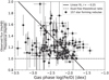 |
Fig. A.1 Comparison of ratios between the observed and theoretical Hα/Hβ fluxes with the gas-phase Fe/O values analyzed in this manuscript for a subsample with reported flux values prior to reddening correction. |
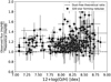 |
Fig. A.3 Comparison of ratios between the observed and theoretical Hα/Hβ fluxes with the 12+log(O/H) values for a subsample of the DESIRED database with reported flux values prior to reddening corrections. |
Appendix B The impact of extrapolating Te-Te relations in the Fe/O and Fe/N distributions
Due to their ionization potential, Fe2+, O+, and N+ are considered low ionization degree ions. This implies that determining their ionic abundances requires adopting a characteristic temperature for their coexistence volume. Various studies indicate that one of the most reliable diagnostics for this parameter is Te([N II] λ5755/λ16584) due to its low dependence on ne (Esteban et al. 2009; Arellano-Córdova & Rodríguez 2020; Méndez-Delgado et al. 2023b; Rickards Vaught et al. 2024). However, observationally, the detection of [N II] λ5755 is particularly challenging for low metallicity regions, which often exhibit high ionization states (Vilchez & Pagel 1988). Because of this, in most cases, a temperature relation is required to connect other temperature diagnostics with Te([N II] λ15755/λ16584). As described in Sect. 2, this work adopted the relations proposed by Garnett (1992) and Méndez-Delgado et al. (2023a) to connect Te([O III] λ14363/λ15007) and/or Te([S III] λ6312/λ9069) when Te([N II] λ15755/λ16584) was not measured directly both in the case t2 = 0 and t2 > 0, respectively.
The use of these temperature relations is a potential source of systematic errors if they have significant deviations from what is present in real nebulae. Although this has been studied in several articles (Skillman et al. 2003; Croxall et al. 2015; Berg et al. 2020; Rogers et al. 2021), both in the case of t2 = 0 (Garnett 1992) and in the case of t2 > 0 (Méndez-Delgado et al. 2023a), there is a very limited number of low-metallicity regions with simultaneous determinations of Te([N II] λ5755/λ16584) and Te([O III] λ14363/λ15007) or Te([S III] λ16312/λ19069). These limitations will be alleviated in upcoming studies (Orte-García M. et al., in prep.) using the DESIRED sample, but the calibrations still lack statistical robustness for temperatures above 13,000K.
To quantify the impact that a hypothetical systematic deviation between the assumed temperature relations and those actually present in the nebulae could have on our determinations of Fe/N and Fe/O abundances, we can consider the following relation (Stasińska 2023):
![Mathematical equation: ${{{\rm{F}}{{\rm{e}}^{2 + }}} \over {{{\rm{O}}^ + }}} = {{\left( {{{I\left( {\left[ {{\rm{Fe}}\,\,{\rm{III}}} \right]\lambda 4658} \right)} \over {I\left( {\left[ {{\rm{O}}\,\,{\rm{II}}} \right]\lambda 3727 + 3729} \right)}}} \right)} \over {\left( {{{j([{\rm{Fe}}\,\,{\rm{III}}]\lambda 4658)} \over {j\left( {\left[ {{\rm{O}}\,\,{\rm{II}}} \right]\lambda \lambda 3727 + 3729} \right)}}} \right)}},$](/articles/aa/full_html/2024/10/aa50928-24/aa50928-24-eq39.png) (B.1)
(B.1)
where I(λ) represents the observed line intensity and j(λ) is the emissivity of that line. In most cases, [O II] λλ3727 + 3729 is the basis for estimating the abundances of O+/H+, and [Fe III] λ4658 is the basis for estimating the abundance of Fe2+/H+ in all cases. If Te([N II]) presents a systematic error, it will affect both j([O II]/λλ3727 + 3729) and j([Fe III]λ4658). We can quantify that systematic error using PyNeb (Luridiana et al. 2015) and Eq. (B.1) as follows:
![Mathematical equation: ${{{{\left( {{\rm{F}}{{\rm{e}}^{2 + }}/{{\rm{O}}^ + }} \right)}_{{\rm{Biased - }}{T_e}}}} \over {{{\left( {{\rm{F}}{{\rm{e}}^{2 + }}/{{\rm{O}}^ + }} \right)}_{{\rm{True - }}{T_e}}}}} = {{{{\left( {{{j([{\rm{FeIII}}]\lambda 4658)} \over {j\left( {\left[ {{\rm{O}}\,{\rm{II}}} \right]\lambda \lambda 3727 + 3729} \right)}}} \right)}_{{\rm{True - }}{T_e}}}} \over {{{\left( {{{j([{\rm{Fe III }}]\lambda 4658)} \over {j([{\rm{O}}\,{\rm{II}}]\lambda 3727 + 3729)}}} \right)}_{{\rm{Biased - }}{T_e}}}}}.$](/articles/aa/full_html/2024/10/aa50928-24/aa50928-24-eq40.png) (B.2)
(B.2)
We consider the following case: In low-metallicity regions, only Te([O III]) is available and we must use the relationships from Garnett (1992) and Méndez-Delgado et al. (2023a) to determine Te([N II]) and T0(O2+). We also assume that the Te relationships induce a systematic error of 20%. This value is notably higher than the uncertainties in the slope and intercept of the Te([O III]) - Te([N II]) relations derived by Méndez-Delgado et al. (2023b) and Te([N II]) - T0 (O2+) derived by Méndez-Delgado et al. (2023a), which are around ~5% in the slopes and ~10% in the intercepts.
In Fig. B.1 it is shown that the potential impact of a systematic error in Te of 20% on the ionic abundance of Fe2+/O+ is ~0.05 dex when adopting the nebular lines [O II]/λλ3727 + 3729. In this figure, ne = 100 cm−3 was considered, although the conclusions do not depend on the value of this parameter. Despite considering systematic errors of several thousand degrees Kelvin, the impact on Fe2+/O+ is very small due to the similarity between the excitation energies of the 3F4 atomic level of Fe2+ (~2.7 eV) and the 2D levels of O+ (~3.3 eV). The same is true for the abundance of Fe2+/N+ (we used [N IJ] 6584, which arises from the 1D level of N+ (~1.9 eV)) as shown in Fig. B.2.
As shown in Fig. B.3, the situation is notably different when the abundance of O+ has been determined using the auroral lines of [O II] λλ7319 + 7320 + 7330 + 7331. The temperature dependence becomes very significant, potentially introducing systematic errors greater than ~0.1 dex. However, only 44 regions (<10% of the entire sample) have O+ determinations based on these auroral lines of [O II]. In Fig. B.4 we demonstrate that these regions do not exhibit anomalies in the observed trends and that our conclusions do not rely particularly on these regions.
To explore the bias in the total abundances of Fe/O and Fe/N, it is necessary to consider the ICF and its relationship with the ionic abundances of O+ and O2+, both in the case of t2 = 0 and t2 > 0. In the case of ICF(Fe), we consider the ICF by Rodríguez & Rubin (2005). As shown in Figs. B.5 and B.6, the potential systematic error is smaller than ~0.04 dex and acts in the opposite direction to the systematic error in the Fe2+/O+ abundance presented in Fig. B.1, which causes the systematic errors to partially cancel each other when determining Fe/O = ICF × Fe2+/O+.
Considering Figs. B.1, B.5, and B.6, we can estimate the total impact of a hypothetical bias in Te on the Fe/O abundances. This is shown in Figs. B.7 and B.8. These figures demonstrate that the potential systematic error induced in the Fe/O abundances due to very large hypothetical errors in Te from the extrapolation of the temperature relationships by Garnett (1992) and Méndez-Delgado et al. (2023a) in low-metallicity regions is around ~0.05 dex. This rules out the possibility that the apparent plateau observed in the Fe/O distribution at low metallicities (see Fig. 6) is the result of a systematic error in the inferred Te([N II]).
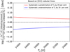 |
Fig. B.1 Upper limits to the systematic errors in the abundance of Fe2+/O+ considering a hypothetical systematic error in Te of 20%. These limits have been calculated using PyNeb (Luridiana et al. 2015) and Eq. (B.2). |
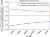 |
Fig. B.3 Same as Fig. B.1 but considering the determination of the O+/H+ ionic abundances based on the [O II] λλ7319 + 7320 + 7330 + 7331 auroral lines. |
The case of the total Fe/N abundance involves two ICFs: the one from Rodríguez & Rubin (2005) for Fe and the one from Amayo et al. (2021) for N. In the latter case, the equation is a fifth-degree polynomial over ω = O2+/(O+ + O2+). For low metallicity regions, ω is expected to be close to 1 (Vilchez & Pagel 1988), minimizing any potential bias in the ionic abundances induced by Te-errors. As a good approximation, we can assume that the ICF(N) induce a negligible systematic error due to systematics on Te. Such case is presented in figures B.9 and B.10 for the case t2 = 0 and t2 > 0, respectively. The potential systematic bias in the Fe/N distribution is rather similar than in the case of Fe/O, being up to ~0.05 dex.
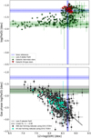 |
Fig. B.4 Same as Fig. 6 but highlighting the subset of objects where the determination of the O+ abundance relies on the [O II] auroral lines. |
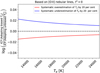 |
Fig. B.5 Upper limits to the systematic errors in ICF(Fe) from Rodríguez & Rubin (2005) considering a hypothetical systematic error in Te of 20%. These limits have been calculated using PyNeb (Luridiana et al. 2015) and Eq. (B.2). |
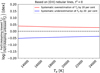 |
Fig. B.7 Same as Fig. B.1 but considering Fe/O=ICF × Fe2+/O+ and the propagation of their corresponding systematic errors under the case t2 = 0. |
Appendix C Fe/O and Fe/N distributions considering t2 = 0
The shape of the Fe/O and Fe/N distributions does not change in the case of t2 = 0. In these cases, the observational fits to the star-forming nebulae are as follows:
For 12+log(O/H) < 7.6:

For 12+log(O/H) ≥ 7.6:
![Mathematical equation: $\log ({\rm{Fe}}/{\rm{O}}) = ( - 1.02 \pm 0.05) \times [12 + \log ({\rm{O}}/{\rm{H}})] + (5.97 \pm 0.39)$](/articles/aa/full_html/2024/10/aa50928-24/aa50928-24-eq42.png)
For 12+log(N/H) < 6.3:

For 12+log(N/H) ≥ 6.3:
![Mathematical equation: $\log ({\rm{Fe}}/{\rm{N}}) = ( - 0.91 \pm 0.03) \times [12 + \log ({\rm{N}}/{\rm{H}})] + (5.20 \pm 0.20)$](/articles/aa/full_html/2024/10/aa50928-24/aa50928-24-eq44.png)
This results in Eq (C.1).
 (C.1)
(C.1)
Appendix D Source data and references
The references for the spectroscopic data are from the following articles: Arellano-Córdova et al. (2021), Berg et al. (2013, 2015, 2020, 2021), Bresolin (2007), Croxall et al. (2015, 2016), Delgado-Inglada et al. (2016), Domínguez-Guzmán et al. (2022), Egorova et al. (2021), Esteban et al. (2004, 2009, 2013, 2014, 2017); Esteban & García-Rojas (2018); Esteban et al. (2020), Fernández et al. (2018, 2022), Fernández-Martín et al. (2017), García-Rojas et al. (2004, 2005, 2006, 2007), Gómez-González et al. (2024), Guseva et al. (2009, 2011, 2024), Hägele et al. (2006, 2008, 2011, 2012), Isobe et al. (2022), Izotov et al. (1997); Izotov & Thuan (1998); Izotov et al. (1999); Izotov & Thuan (2004); Izotov et al. (2006); Izotov et al. (2009, 2012, 2017, 2018, 2021), Kojima et al. (2021), López-Sánchez et al. (2007, 2015), Méndez-Delgado et al. (2021a); Méndez-Delgado et al. (2021b, 2022b), Mesa-Delgado et al. (2009), Peimbert (2003); Peimbert et al. (2005); Peimbert et al. (2012), Peña-Guerrero et al. (2012), Rogers et al. (2021, 2022), Skillman (1985), Thuan & Izotov (2005), Toribio San Cipriano et al. (2016), Valerdi et al. (2019, 2021), Watanabe et al. (2024), Welch et al. (2024) and Zurita & Bresolin (2012).
The atomic data used are as follows: O+: Froese Fischer & Tachiev (2004), Kisielius et al. (2009); O2+: Wiese et al. (1996), Storey & Zeippen (2000), Storey et al. (2014); N+: Froese Fischer & Tachiev (2004), Tayal (2011); S+: Irimia & Froese Fischer (2005), Tayal & Zatsarinny (2010); S2+: Froese Fischer et al. (2006), Grieve et al. (2014); Cl2+: Fritzsche et al. (1999), Butler & Zeippen (1989); Ar2+: Mendoza (1983), Kaufman & Sugar (1986), Galavis et al. (1995); Ar3+: Mendoza & Zeippen (1982), Ramsbottom & Bell (1997); Fe+: Bautista et al. (2015), Mendoza et al. (2023); Fe2+: Deb & Hibbert (2009), Mendoza et al. (2023), Zhang (1996); Fe3+: Froese Fischer et al. (2008), Zhang & Pradhan (1997); Fe4+: Nahar et al. (2000), Ballance et al. (2007).
The calculations and complete reference tables associated with Appendix D mentioned in this article can be found at: https://zenodo.org/records/13380667.
References
- Abazajian, K., Adelman-McCarthy, J. K., Agüeros, M. A., et al. 2005, AJ, 129, 1755 [NASA ADS] [CrossRef] [Google Scholar]
- Amarsi, A. M., Nissen, P. E., Asplund, M., Lind, K., & Barklem, P. S. 2019, A&A, 622, L4 [NASA ADS] [CrossRef] [EDP Sciences] [Google Scholar]
- Amarsi, A. M., Grevesse, N., Grumer, J., et al. 2020, A&A, 636, A120 [NASA ADS] [CrossRef] [EDP Sciences] [Google Scholar]
- Amarsi, A. M., Grevesse, N., Asplund, M., & Collet, R. 2021, A&A, 656, A113 [NASA ADS] [CrossRef] [EDP Sciences] [Google Scholar]
- Amayo, A., Delgado-Inglada, G., & Stasinska, G. 2021, MNRAS, 505, 2361 [CrossRef] [Google Scholar]
- Arellano-Córdova, K. Z., & Rodríguez, M. 2020, MNRAS, 497, 672 [CrossRef] [Google Scholar]
- Arellano-Córdova, K. Z., Esteban, C., García-Rojas, J., & Méndez-Delgado, J. E. 2020, MNRAS, 496, 1051 [Google Scholar]
- Arellano-Córdova, K. Z., Esteban, C., García-Rojas, J., & Méndez-Delgado, J. E. 2021, MNRAS, 502, 225 [CrossRef] [Google Scholar]
- Arellano-Córdova, K. Z., Berg, D. A., Chisholm, J., et al. 2022, ApJ, 940, L23 [CrossRef] [Google Scholar]
- Arellano-Córdova, K. Z., Berg, D. A., Mingozzi, M., et al. 2024, arXiv e-prints [arXiv:2403.08401] [Google Scholar]
- Asplund, M. 2005, ARA&A, 43, 481 [Google Scholar]
- Asplund, M., Amarsi, A. M., & Grevesse, N. 2021, A&A, 653, A141 [NASA ADS] [CrossRef] [EDP Sciences] [Google Scholar]
- Aver, E., Olive, K. A., & Skillman, E. D. 2015, J. Cosmology Astropart. Phys., 2015, 011 [Google Scholar]
- Baldwin, J. A., Phillips, M. M., & Terlevich, R. 1981, PASP, 93, 5 [Google Scholar]
- Baldwin, J. A., Crotts, A., Dufour, R. J., et al. 1996, ApJ, 468, L115 [NASA ADS] [CrossRef] [Google Scholar]
- Ballance, C. P., Griffin, D. C., & McLaughlin, B. M. 2007, J. Phys. B At. Mol. Phys., 40, F327 [CrossRef] [Google Scholar]
- Bautista, M. A., Fivet, V., Ballance, C., et al. 2015, ApJ, 808, 174 [NASA ADS] [CrossRef] [Google Scholar]
- Bensby, T., Yee, J. C., Feltzing, S., et al. 2013, A&A, 549, A147 [NASA ADS] [CrossRef] [EDP Sciences] [Google Scholar]
- Berg, D. A., Skillman, E. D., Garnett, D. R., et al. 2013, ApJ, 775, 128 [NASA ADS] [CrossRef] [Google Scholar]
- Berg, D. A., Skillman, E. D., Croxall, K. V., et al. 2015, ApJ, 806, 16 [NASA ADS] [CrossRef] [Google Scholar]
- Berg, D. A., Pogge, R. W., Skillman, E. D., et al. 2020, ApJ, 893, 96 [NASA ADS] [CrossRef] [Google Scholar]
- Berg, D. A., Chisholm, J., Erb, D. K., et al. 2021, ApJ, 922, 170 [CrossRef] [Google Scholar]
- Bergerud, B. M., Spangler, S. R., & Beauchamp, K. M. 2020, MNRAS, 492, 1142 [NASA ADS] [CrossRef] [Google Scholar]
- Blagrave, K. P. M., Martin, P. G., & Baldwin, J. A. 2006, ApJ, 644, 1006 [NASA ADS] [CrossRef] [Google Scholar]
- Bocchio, M., Jones, A. P., & Slavin, J. D. 2014, A&A, 570, A32 [NASA ADS] [CrossRef] [EDP Sciences] [Google Scholar]
- Bragança, G. A., Daflon, S., Lanz, T., et al. 2019, A&A, 625, A120 [NASA ADS] [CrossRef] [EDP Sciences] [Google Scholar]
- Bresolin, F. 2007, ApJ, 656, 186 [NASA ADS] [CrossRef] [Google Scholar]
- Bresolin, F., Schaerer, D., González Delgado, R. M., & Stasinska, G. 2005, A&A, 441, 981 [NASA ADS] [CrossRef] [EDP Sciences] [Google Scholar]
- Bresolin, F., Gieren, W., Kudritzki, R.-P., et al. 2009, ApJ, 700, 309 [NASA ADS] [CrossRef] [Google Scholar]
- Bresolin, F., Kudritzki, R.-P., Urbaneja, M. A., et al. 2016, ApJ, 830, 64 [NASA ADS] [CrossRef] [Google Scholar]
- Bresolin, F., Kudritzki, R.-P., & Urbaneja, M. A. 2022, ApJ, 940, 32 [NASA ADS] [CrossRef] [Google Scholar]
- Butler, K., & Zeippen, C. J. 1989, A&A, 208, 337 [NASA ADS] [Google Scholar]
- Calzetti, D., Kinney, A. L., & Storchi-Bergmann, T. 1994, ApJ, 429, 582 [Google Scholar]
- Cameron, A. J., Katz, H., & Rey, M. P. 2023, MNRAS, 522, L89 [NASA ADS] [CrossRef] [Google Scholar]
- Carigi, L., Peimbert, M., Esteban, C., & García-Rojas, J. 2005, ApJ, 623, 213 [NASA ADS] [CrossRef] [Google Scholar]
- Carigi, L., Peimbert, M., & Peimbert, A. 2019, ApJ, 873, 107 [NASA ADS] [CrossRef] [Google Scholar]
- Carretta, E., Gratton, R. G., & Sneden, C. 2000, A&A, 356, 238 [Google Scholar]
- Castellanos, M., Díaz, A. I., & Terlevich, E. 2002, MNRAS, 329, 315 [CrossRef] [Google Scholar]
- Cayrel, R., Depagne, E., Spite, M., et al. 2004, A&A, 416, 1117 [NASA ADS] [CrossRef] [EDP Sciences] [Google Scholar]
- Chiappini, C., Romano, D., & Matteucci, F. 2003, MNRAS, 339, 63 [NASA ADS] [CrossRef] [Google Scholar]
- Choban, C. R., Kereš, D., Hopkins, P. F., et al. 2022, MNRAS, 514, 4506 [NASA ADS] [CrossRef] [Google Scholar]
- Chruślińska, M., Pakmor, R., Matthee, J., & Matsuno, T. 2024, A&A, 686, A186 [NASA ADS] [CrossRef] [EDP Sciences] [Google Scholar]
- Crowther, P. A. 2007, ARA&A, 45, 177 [Google Scholar]
- Croxall, K. V., Pogge, R. W., Berg, D. A., Skillman, E. D., & Moustakas, J. 2015, ApJ, 808, 42 [NASA ADS] [CrossRef] [Google Scholar]
- Croxall, K. V., Pogge, R. W., Berg, D. A., Skillman, E. D., & Moustakas, J. 2016, ApJ, 830, 4 [NASA ADS] [CrossRef] [Google Scholar]
- Curti, M., Cresci, G., Mannucci, F., et al. 2017, MNRAS, 465, 1384 [Google Scholar]
- Deb, N. C., & Hibbert, A. 2009, At. Data Nucl. Data Tables, 95, 184 [NASA ADS] [CrossRef] [Google Scholar]
- Delgado-Inglada, G., Mesa-Delgado, A., García-Rojas, J., Rodríguez, M., & Esteban, C. 2016, MNRAS, 456, 3855 [NASA ADS] [CrossRef] [Google Scholar]
- Dinerstein, H. L. 1990, in Astrophysics and Space Science Library, 161, The Interstellar Medium in Galaxies, eds. J. Thronson, A. Harley, & J. M. Shull, 257 [NASA ADS] [CrossRef] [Google Scholar]
- Domínguez-Guzmán, G., Rodríguez, M., García-Rojas, J., Esteban, C., & Toribio San Cipriano, L. 2022, MNRAS, 517, 4497 [CrossRef] [Google Scholar]
- Drory, N., Blanc, G. A., Kreckel, K., et al. 2024, arXiv e-prints [arXiv:2405.01637] [Google Scholar]
- Dubois, Y., Rodríguez Montero, F., Guerra, C., et al. 2024, A&A, 687, A240 [NASA ADS] [CrossRef] [EDP Sciences] [Google Scholar]
- Ecuvillon, A., Israelian, G., Santos, N. C., et al. 2004, A&A, 418, 703 [NASA ADS] [CrossRef] [EDP Sciences] [Google Scholar]
- Egorova, E. S., Egorov, O. V., Moiseev, A. V., et al. 2021, MNRAS, 504, 6179 [CrossRef] [Google Scholar]
- Espíritu, J. N., Peimbert, A., Delgado-Inglada, G., & Ruiz, M. T. 2017, Rev. Mexicana Astron. Astrofis., 53, 95 [Google Scholar]
- Esteban, C., & García-Rojas, J. 2018, MNRAS, 478, 2315 [NASA ADS] [CrossRef] [Google Scholar]
- Esteban, C., Peimbert, M., Torres-Peimbert, S., & Rodríguez, M. 2002, ApJ, 581, 241 [NASA ADS] [CrossRef] [Google Scholar]
- Esteban, C., Peimbert, M., García-Rojas, J., et al. 2004, MNRAS, 355, 229 [NASA ADS] [CrossRef] [Google Scholar]
- Esteban, C., Bresolin, F., Peimbert, M., et al. 2009, ApJ, 700, 654 [NASA ADS] [CrossRef] [Google Scholar]
- Esteban, C., Carigi, L., Copetti, M. V. F., et al. 2013, MNRAS, 433, 382 [NASA ADS] [CrossRef] [Google Scholar]
- Esteban, C., García-Rojas, J., Carigi, L., et al. 2014, MNRAS, 443, 624 [NASA ADS] [CrossRef] [Google Scholar]
- Esteban, C., Mesa-Delgado, A., Morisset, C., & García-Rojas, J. 2016, MNRAS, 460, 4038 [NASA ADS] [CrossRef] [Google Scholar]
- Esteban, C., Fang, X., García-Rojas, J., & Toribio San Cipriano, L. 2017, MNRAS, 471, 987 [NASA ADS] [CrossRef] [Google Scholar]
- Esteban, C., Bresolin, F., García-Rojas, J., & Toribio San Cipriano, L. 2020, MNRAS, 491, 2137 [NASA ADS] [Google Scholar]
- Esteban, C., Méndez-Delgado, J. E., García-Rojas, J., & Arellano-Córdova, K. Z. 2022, ApJ, 931, 92 [NASA ADS] [CrossRef] [Google Scholar]
- Evans, C. J., Bresolin, F., Urbaneja, M. A., et al. 2007, ApJ, 659, 1198 [Google Scholar]
- Ferland, G. J., Chatzikos, M., Guzmán, F., et al. 2017, Rev. Mexicana Astron. Astrofis., 53, 385 [Google Scholar]
- Fernández, V., Terlevich, E., Díaz, A. I., Terlevich, R., & Rosales-Ortega, F. F. 2018, MNRAS, 478, 5301 [CrossRef] [Google Scholar]
- Fernández, V., Amorín, R., Pérez-Montero, E., et al. 2022, MNRAS, 511, 2515 [CrossRef] [Google Scholar]
- Fernández-Martín, A., Pérez-Montero, E., Vílchez, J. M., & Mampaso, A. 2017, A&A, 597, A84 [NASA ADS] [CrossRef] [EDP Sciences] [Google Scholar]
- Fritzsche, S., Fricke, B., Geschke, D., Heitmann, A., & Sienkiewicz, J. E. 1999, ApJ, 518, 994 [NASA ADS] [CrossRef] [Google Scholar]
- Froese Fischer, C., & Tachiev, G. 2004, At. Data Nucl. Data Tables, 87, 1 [NASA ADS] [CrossRef] [Google Scholar]
- Froese Fischer, C., Tachiev, G., & Irimia, A. 2006, At. Data Nucl. Data Tables, 92, 607 [NASA ADS] [CrossRef] [Google Scholar]
- Froese Fischer, C., Rubin, R. H., & Rodríguez, M. 2008, MNRAS, 391, 1828 [NASA ADS] [CrossRef] [Google Scholar]
- Galavis, M. E., Mendoza, C., & Zeippen, C. J. 1995, A&AS, 111, 347 [Google Scholar]
- Galliano, F., Nersesian, A., Bianchi, S., et al. 2021, A&A, 649, A18 [EDP Sciences] [Google Scholar]
- Garcia, M., Herrero, A., Najarro, F., Lennon, D. J., & Alejandro Urbaneja, M. 2014, ApJ, 788, 64 [NASA ADS] [CrossRef] [Google Scholar]
- García-Rojas, J., & Esteban, C. 2007, ApJ, 670, 457 [CrossRef] [Google Scholar]
- García-Rojas, J., Esteban, C., Peimbert, M., et al. 2004, ApJS, 153, 501 [CrossRef] [Google Scholar]
- García-Rojas, J., Esteban, C., Peimbert, A., et al. 2005, MNRAS, 362, 301 [CrossRef] [Google Scholar]
- García-Rojas, J., Esteban, C., Peimbert, M., et al. 2006, MNRAS, 368, 253 [CrossRef] [Google Scholar]
- García-Rojas, J., Esteban, C., Peimbert, A., et al. 2007, Rev. Mexicana Astron. Astrofis., 43, 3 [Google Scholar]
- García-Rojas, J., Simón-Díaz, S., & Esteban, C. 2014, A&A, 571, A93 [NASA ADS] [CrossRef] [EDP Sciences] [Google Scholar]
- Garnett, D. R. 1990, ApJ, 363, 142 [NASA ADS] [CrossRef] [Google Scholar]
- Garnett, D. R. 1992, AJ, 103, 1330 [NASA ADS] [CrossRef] [Google Scholar]
- Gazak, J. Z., Kudritzki, R., Evans, C., et al. 2015, ApJ, 805, 182 [NASA ADS] [CrossRef] [Google Scholar]
- Gioannini, L., Matteucci, F., Vladilo, G., & Calura, F. 2017, MNRAS, 464, 985 [CrossRef] [Google Scholar]
- Gómez-González, V. M. A., Mayya, Y. D., Zaragoza-Cardiel, J., et al. 2024, MNRAS, 529, 4369 [CrossRef] [Google Scholar]
- Goswami, S., Slemer, A., Marigo, P., et al. 2021, A&A, 650, A203 [NASA ADS] [CrossRef] [EDP Sciences] [Google Scholar]
- Goswami, S., Silva, L., Bressan, A., et al. 2022, A&A, 663, A1 [NASA ADS] [CrossRef] [EDP Sciences] [Google Scholar]
- Gratton, R. G., Carretta, E., Matteucci, F., & Sneden, C. 2000, A&A, 358, 671 [NASA ADS] [Google Scholar]
- Greggio, L. 2005, A&A, 441, 1055 [NASA ADS] [CrossRef] [EDP Sciences] [Google Scholar]
- Grieve, M. F. R., Ramsbottom, C. A., Hudson, C. E., & Keenan, F. P. 2014, ApJ, 780, 110 [Google Scholar]
- Grisoni, V., Matteucci, F., & Romano, D. 2021, MNRAS, 508, 719 [NASA ADS] [CrossRef] [Google Scholar]
- Gunasekera, C. M., Ji, X., Chatzikos, M., Yan, R., & Ferland, G. 2023, MNRAS, 520, 4345 [NASA ADS] [CrossRef] [Google Scholar]
- Guseva, N. G., Papaderos, P., Meyer, H. T., Izotov, Y. I., & Fricke, K. J. 2009, A&A, 505, 63 [NASA ADS] [CrossRef] [EDP Sciences] [Google Scholar]
- Guseva, N. G., Izotov, Y. I., Stasin´ska, G., et al. 2011, A&A, 529, A149 [NASA ADS] [CrossRef] [EDP Sciences] [Google Scholar]
- Guseva, N. G., Thuan, T. X., & Izotov, Y. I. 2024, MNRAS, 527, 3932 [Google Scholar]
- Hägele, G. F., Pérez-Montero, E., Díaz, Á. I., Terlevich, E., & Terlevich, R. 2006, MNRAS, 372, 293 [CrossRef] [Google Scholar]
- Hägele, G. F., Díaz, Á. I., Terlevich, E., et al. 2008, MNRAS, 383, 209 [Google Scholar]
- Hägele, G. F., García-Benito, R., Pérez-Montero, E., et al. 2011, MNRAS, 414, 272 [CrossRef] [Google Scholar]
- Hägele, G. F., Firpo, V., Bosch, G., Díaz, Á. I., & Morrell, N. 2012, MNRAS, 422, 3475 [NASA ADS] [CrossRef] [Google Scholar]
- Hendricks, B., Koch, A., Lanfranchi, G. A., et al. 2014, ApJ, 785, 102 [NASA ADS] [CrossRef] [Google Scholar]
- Henry, R. B. C., Edmunds, M. G., & Köppen, J. 2000, ApJ, 541, 660 [NASA ADS] [CrossRef] [Google Scholar]
- Hensley, B. S., & Draine, B. T. 2023, ApJ, 948, 55 [Google Scholar]
- Higgins, E. R., Vink, J. S., Hirschi, R., Laird, A. M., & Sabhahit, G. N. 2023, MNRAS, 526, 534 [NASA ADS] [CrossRef] [Google Scholar]
- Hill, V., Skúladóttir, Á., Tolstoy, E., et al. 2019, A&A, 626, A15 [NASA ADS] [CrossRef] [EDP Sciences] [Google Scholar]
- Hosek, Matthew W., J., Kudritzki, R.-P., Bresolin, F., et al. 2014, ApJ, 785, 151 [NASA ADS] [CrossRef] [Google Scholar]
- Hsyu, T., Cooke, R. J., Prochaska, J. X., & Bolte, M. 2020, ApJ, 896, 77 [NASA ADS] [CrossRef] [Google Scholar]
- Hunter, I., Dufton, P. L., Smartt, S. J., et al. 2007, A&A, 466, 277 [NASA ADS] [CrossRef] [EDP Sciences] [Google Scholar]
- Irimia, A., & Froese Fischer, C. 2005, Phys. Scr, 71, 172 [NASA ADS] [CrossRef] [Google Scholar]
- Isobe, Y., Ouchi, M., Suzuki, A., et al. 2022, ApJ, 925, 111 [NASA ADS] [CrossRef] [Google Scholar]
- Israelian, G., Ecuvillon, A., Rebolo, R., et al. 2004, A&A, 421, 649 [NASA ADS] [CrossRef] [EDP Sciences] [Google Scholar]
- Izotov, Y. I., & Thuan, T. X. 1998, ApJ, 500, 188 [NASA ADS] [CrossRef] [Google Scholar]
- Izotov, Y. I., & Thuan, T. X. 1999, ApJ, 511, 639 [NASA ADS] [CrossRef] [Google Scholar]
- Izotov, Y. I., & Thuan, T. X. 2004, ApJ, 602, 200 [CrossRef] [Google Scholar]
- Izotov, Y. I., Thuan, T. X., & Lipovetsky, V. A. 1997, ApJS, 108, 1 [NASA ADS] [CrossRef] [Google Scholar]
- Izotov, Y. I., Chaffee, F. H., Foltz, C. B., et al. 1999, ApJ, 527, 757 [NASA ADS] [CrossRef] [Google Scholar]
- Izotov, Y. I., Stasin´ ska, G., Meynet, G., Guseva, N. G., & Thuan, T. X. 2006, A&A, 448, 955 [CrossRef] [EDP Sciences] [Google Scholar]
- Izotov, Y. I., Guseva, N. G., Fricke, K. J., & Papaderos, P. 2009, A&A, 503, 61 [NASA ADS] [CrossRef] [EDP Sciences] [Google Scholar]
- Izotov, Y. I., Thuan, T. X., & Privon, G. 2012, MNRAS, 427, 1229 [NASA ADS] [CrossRef] [Google Scholar]
- Izotov, Y. I., Thuan, T. X., & Guseva, N. G. 2017, MNRAS, 471, 548 [NASA ADS] [CrossRef] [Google Scholar]
- Izotov, Y. I., Thuan, T. X., Guseva, N. G., & Liss, S. E. 2018, MNRAS, 473, 1956 [NASA ADS] [CrossRef] [Google Scholar]
- Izotov, Y. I., Thuan, T. X., & Guseva, N. G. 2021, MNRAS, 508, 2556 [NASA ADS] [CrossRef] [Google Scholar]
- Jenkins, E. B. 2009, ApJ, 700, 1299 [Google Scholar]
- Ji, X., Übler, H., Maiolino, R., et al. 2024, arXiv e-prints [arXiv:2404.04148] [Google Scholar]
- Jones, A. P., Köhler, M., Ysard, N., Bocchio, M., & Verstraete, L. 2017, A&A, 602, A46 [NASA ADS] [CrossRef] [EDP Sciences] [Google Scholar]
- Kaufman, V., & Sugar, J. 1986, J. Phys. Chem. Ref. Data, 15, 321 [NASA ADS] [CrossRef] [Google Scholar]
- Kauffmann, G., Heckman, T. M., Tremonti, C., et al. 2003, MNRAS, 346, 1055 [Google Scholar]
- Kennicutt, Robert C., J., Bresolin, F., & Garnett, D. R. 2003, ApJ, 591, 801 [NASA ADS] [CrossRef] [Google Scholar]
- Kirchschlager, F., Mattsson, L., & Gent, F. A. 2022, MNRAS, 509, 3218 [Google Scholar]
- Kirchschlager, F., Sartorio, N. S., De Looze, I., et al. 2024, MNRAS, 528, 5364 [NASA ADS] [CrossRef] [Google Scholar]
- Kisielius, R., Storey, P. J., Ferland, G. J., & Keenan, F. P. 2009, MNRAS, 397, 903 [NASA ADS] [CrossRef] [Google Scholar]
- Kobayashi, C., Umeda, H., Nomoto, K., Tominaga, N., & Ohkubo, T. 2006, ApJ, 653, 1145 [NASA ADS] [CrossRef] [Google Scholar]
- Kobayashi, C., Karakas, A. I., & Lugaro, M. 2020, ApJ, 900, 179 [Google Scholar]
- Kojima, T., Ouchi, M., Rauch, M., et al. 2021, ApJ, 913, 22 [NASA ADS] [CrossRef] [Google Scholar]
- Kudritzki, R.-P., Urbaneja, M. A., Bresolin, F., et al. 2008, ApJ, 681, 269 [NASA ADS] [CrossRef] [Google Scholar]
- Kudritzki, R.-P., Urbaneja, M. A., Gazak, Z., et al. 2012, ApJ, 747, 15 [CrossRef] [Google Scholar]
- Kudritzki, R.-P., Urbaneja, M. A., Bresolin, F., Hosek, Matthew W., J., & Przybilla, N. 2014, ApJ, 788, 56 [NASA ADS] [CrossRef] [Google Scholar]
- Kudritzki, R. P., Castro, N., Urbaneja, M. A., et al. 2016, ApJ, 829, 70 [NASA ADS] [CrossRef] [Google Scholar]
- Kurichin, O. A., Kislitsyn, P. A., Klimenko, V. V., Balashev, S. A., & Ivanchik, A. V. 2021, MNRAS, 502, 3045 [NASA ADS] [CrossRef] [Google Scholar]
- Kwitter, K. B. 1984, ApJ, 287, 840 [NASA ADS] [CrossRef] [Google Scholar]
- Limongi, M., & Chieffi, A. 2018, ApJS, 237, 13 [NASA ADS] [CrossRef] [Google Scholar]
- Lin, Z., Hu, N., Kong, X., et al. 2017, ApJ, 842, 97 [NASA ADS] [CrossRef] [Google Scholar]
- López-Sánchez, A. R., & Esteban, C. 2009, A&A, 508, 615 [NASA ADS] [CrossRef] [EDP Sciences] [Google Scholar]
- López-Sánchez, Á. R., Esteban, C., García-Rojas, J., Peimbert, M., & Rodríguez, M. 2007, ApJ, 656, 168 [CrossRef] [Google Scholar]
- López-Sánchez, Á. R., Westmeier, T., Esteban, C., & Koribalski, B. S. 2015, MNRAS, 450, 3381 [CrossRef] [Google Scholar]
- Luridiana, V., Morisset, C., & Shaw, R. A. 2015, A&A, 573, A42 [NASA ADS] [CrossRef] [EDP Sciences] [Google Scholar]
- Magrini, L., Stanghellini, L., Corbelli, E., Galli, D., & Villaver, E. 2010, A&A, 512, A63 [NASA ADS] [CrossRef] [EDP Sciences] [Google Scholar]
- Magrini, L., Vincenzo, F., Randich, S., et al. 2018, A&A, 618, A102 [NASA ADS] [CrossRef] [EDP Sciences] [Google Scholar]
- Maoz, D., & Mannucci, F. 2012, PASA, 29, 447 [NASA ADS] [CrossRef] [Google Scholar]
- Martins, F., Hervé, A., Bouret, J. C., et al. 2015, A&A, 575, A34 [NASA ADS] [CrossRef] [EDP Sciences] [Google Scholar]
- Martins, F., Bouret, J. C., Hillier, D. J., et al. 2024, arXiv e-prints [arXiv:2405.01267] [Google Scholar]
- Matsumoto, A., Ouchi, M., Nakajima, K., et al. 2022, ApJ, 941, 167 [NASA ADS] [CrossRef] [Google Scholar]
- Matteucci, F. 2012, Chemical Evolution of Galaxies [Google Scholar]
- Matteucci, F., & Greggio, L. 1986, A&A, 154, 279 [NASA ADS] [Google Scholar]
- Méndez-Delgado, J. E., Esteban, C., García-Rojas, J., Arellano-Córdova, K. Z., & Valerdi, M. 2020, MNRAS, 496, 2726 [CrossRef] [Google Scholar]
- Méndez-Delgado, J. E., Esteban, C., García-Rojas, J., et al. 2021a, MNRAS, 502, 1703 [CrossRef] [Google Scholar]
- Méndez-Delgado, J. E., Henney, W. J., Esteban, C., et al. 2021b, ApJ, 918, 27 [CrossRef] [Google Scholar]
- Méndez-Delgado, J. E., Amayo, A., Arellano-Córdova, K. Z., et al. 2022a, MNRAS, 510, 4436 [CrossRef] [Google Scholar]
- Méndez-Delgado, J. E., Esteban, C., García-Rojas, J., & Henney, W. J. 2022b, MNRAS, 514, 744 [CrossRef] [Google Scholar]
- Méndez-Delgado, J. E., Esteban, C., García-Rojas, J., Kreckel, K., & Peimbert, M. 2023a, Nature, 618, 249 [CrossRef] [Google Scholar]
- Méndez-Delgado, J. E., Esteban, C., García-Rojas, J., et al. 2023b, MNRAS, 523, 2952 [CrossRef] [Google Scholar]
- Méndez-Delgado, J. E., Esteban, C., García-Rojas, J., Kreckel, K., & Peimbert, M. 2024, Nat. Astron., 8, 275 [Google Scholar]
- Mendoza, C. 1983, in IAU Symposium, 103, Planetary Nebulae, ed. L. H. Aller, 143 [NASA ADS] [Google Scholar]
- Mendoza, C., & Zeippen, C. J. 1982, MNRAS, 198, 127 [NASA ADS] [Google Scholar]
- Mendoza, C., Méndez-Delgado, J. E., Bautista, M., García-Rojas, J., & Morisset, C. 2023, Atoms, 11, 63 [NASA ADS] [CrossRef] [Google Scholar]
- Mesa-Delgado, A., Esteban, C., García-Rojas, J., et al. 2009, MNRAS, 395, 855 [NASA ADS] [CrossRef] [Google Scholar]
- Meynet, G., & Maeder, A. 2002a, A&A, 390, 561 [NASA ADS] [CrossRef] [EDP Sciences] [Google Scholar]
- Meynet, G., & Maeder, A. 2002b, A&A, 381, L25 [NASA ADS] [CrossRef] [EDP Sciences] [Google Scholar]
- Meynet, G., & Maeder, A. 2005, A&A, 429, 581 [CrossRef] [EDP Sciences] [Google Scholar]
- Mollá, M., Vílchez, J. M., Gavilán, M., & Díaz, A. I. 2006, MNRAS, 372, 1069 [CrossRef] [Google Scholar]
- Morisset, C. 2004, ApJ, 601, 858 [NASA ADS] [CrossRef] [Google Scholar]
- Nahar, S. N., Delahaye, F., Pradhan, A. K., & Zeippen, C. J. 2000, A&AS, 144, 141 [NASA ADS] [CrossRef] [EDP Sciences] [Google Scholar]
- Nava, A., Casebeer, D., Henry, R. B. C., & Jevremovic, D. 2006, ApJ, 645, 1076 [NASA ADS] [CrossRef] [Google Scholar]
- Nicholls, D. C., Sutherland, R. S., Dopita, M. A., Kewley, L. J., & Groves, B. A. 2017, MNRAS, 466, 4403 [Google Scholar]
- Nieva, M. F., & Przybilla, N. 2012, A&A, 539, A143 [NASA ADS] [CrossRef] [EDP Sciences] [Google Scholar]
- Noll, S., Kausch, W., Barden, M., et al. 2012, A&A, 543, A92 [NASA ADS] [CrossRef] [EDP Sciences] [Google Scholar]
- Nomoto, K., Kobayashi, C., & Tominaga, N. 2013, ARA&A, 51, 457 [CrossRef] [Google Scholar]
- Osterbrock, D. E., & Ferland, G. J. 2006, Astrophysics of gaseous nebulae and active galactic nuclei [Google Scholar]
- Osterbrock, D. E., Tran, H. D., & Veilleux, S. 1992, ApJ, 389, 305 [Google Scholar]
- Pagel, B. E. J., Simonson, E. A., Terlevich, R. J., & Edmunds, M. G. 1992, MNRAS, 255, 325 [CrossRef] [Google Scholar]
- Palla, M. 2021, MNRAS, 503, 3216 [Google Scholar]
- Patrick, L. R., Evans, C. J., Davies, B., et al. 2015, ApJ, 803, 14 [Google Scholar]
- Patterson, M. T., Walterbos, R. A. M., Kennicutt, R. C., Chiappini, C., & Thilker, D. A. 2012, MNRAS, 422, 401 [NASA ADS] [CrossRef] [Google Scholar]
- Pauli, D., Oskinova, L. M., Hamann, W. R., et al. 2023, A&A, 673, A40 [NASA ADS] [CrossRef] [EDP Sciences] [Google Scholar]
- Peña, M., Stasin´ska, G., & Richer, M. G. 2007, A&A, 476, 745 [NASA ADS] [CrossRef] [EDP Sciences] [Google Scholar]
- Peña-Guerrero, M. A., Peimbert, A., Peimbert, M., & Ruiz, M. T. 2012, ApJ, 746, 115 [CrossRef] [Google Scholar]
- Peimbert, M. 1967, ApJ, 150, 825 [NASA ADS] [CrossRef] [Google Scholar]
- Peimbert, M. 1971, Bol. Observ. Tonantzintla Tacubaya, 6, 29 [NASA ADS] [Google Scholar]
- Peimbert, A. 2003, ApJ, 584, 735 [NASA ADS] [CrossRef] [Google Scholar]
- Peimbert, M., & Costero, R. 1969, Bol. Observ. Tonantzintla Tacubaya, 5, 3 [NASA ADS] [Google Scholar]
- Peimbert, M., & Torres-Peimbert, S. 1974, ApJ, 193, 327 [NASA ADS] [CrossRef] [Google Scholar]
- Peimbert, A., & Peimbert, M. 2010, ApJ, 724, 791 [NASA ADS] [CrossRef] [Google Scholar]
- Peimbert, A., Peimbert, M., & Luridiana, V. 2002, ApJ, 565, 668 [NASA ADS] [CrossRef] [Google Scholar]
- Peimbert, A., Peimbert, M., & Ruiz, M. T. 2005, ApJ, 634, 1056 [NASA ADS] [CrossRef] [Google Scholar]
- Peimbert, M., Luridiana, V., & Peimbert, A. 2007, ApJ, 666, 636 [NASA ADS] [CrossRef] [Google Scholar]
- Peimbert, A., Peña-Guerrero, M. A., & Peimbert, M. 2012, ApJ, 753, 39 [NASA ADS] [CrossRef] [Google Scholar]
- Peimbert, M., Peimbert, A., & Delgado-Inglada, G. 2017, PASP, 129, 082001 [NASA ADS] [CrossRef] [Google Scholar]
- Pilyugin, L. S., Vílchez, J. M., & Thuan, T. X. 2010, ApJ, 720, 1738 [NASA ADS] [CrossRef] [Google Scholar]
- Prantzos, N., Abia, C., Chen, T., et al. 2023, MNRAS, 523, 2126 [NASA ADS] [CrossRef] [Google Scholar]
- Prantzos, N., Abia, C., Limongi, M., Chieffi, A., & Cristallo, S. 2018, MNRAS, 476, 3432 [Google Scholar]
- Przybilla, N., Firnstein, M., Nieva, M. F., Meynet, G., & Maeder, A. 2010, A&A, 517, A38 [NASA ADS] [CrossRef] [EDP Sciences] [Google Scholar]
- Ramachandran, V., Oskinova, L. M., & Hamann, W. R. 2021, A&A, 646, A16 [NASA ADS] [CrossRef] [EDP Sciences] [Google Scholar]
- Ramsbottom, C. A., & Bell, K. L. 1997, At. Data Nucl. Data Tables, 66, 65 [NASA ADS] [CrossRef] [Google Scholar]
- Rickards Vaught, R. J., Sandstrom, K. M., Belfiore, F., et al. 2024, ApJ, 966, 130 [NASA ADS] [CrossRef] [Google Scholar]
- Rodríguez, M. 1996, A&A, 313, L5 [NASA ADS] [Google Scholar]
- Rodríguez, M. 1999, A&A, 348, 222 [NASA ADS] [Google Scholar]
- Rodríguez, M. 2002, A&A, 389, 556 [NASA ADS] [CrossRef] [EDP Sciences] [Google Scholar]
- Rodríguez, M., & Rubin, R. H. 2005, ApJ, 626, 900 [CrossRef] [Google Scholar]
- Rogers, N. S. J., Skillman, E. D., Pogge, R. W., et al. 2021, ApJ, 915, 21 [NASA ADS] [CrossRef] [Google Scholar]
- Rogers, N. S. J., Skillman, E. D., Pogge, R. W., et al. 2022, ApJ, 939, 44 [NASA ADS] [CrossRef] [Google Scholar]
- Rolleston, W. R. J., Venn, K., Tolstoy, E., & Dufton, P. L. 2003, A&A, 400, 21 [NASA ADS] [CrossRef] [EDP Sciences] [Google Scholar]
- Roman-Duval, J., Jenkins, E. B., Tchernyshyov, K., et al. 2022a, ApJ, 928, 90 [NASA ADS] [CrossRef] [Google Scholar]
- Roman-Duval, J., Jenkins, E. B., Tchernyshyov, K., et al. 2022b, ApJ, 935, 105 [Google Scholar]
- Romano, D., Matteucci, F., Zhang, Z.-Y., Ivison, R. J., & Ventura, P. 2019, MNRAS, 490, 2838 [NASA ADS] [CrossRef] [Google Scholar]
- Rosolowsky, E., & Simon, J. D. 2008, ApJ, 675, 1213 [NASA ADS] [CrossRef] [Google Scholar]
- Rubin, R. H. 1989, ApJS, 69, 897 [NASA ADS] [CrossRef] [Google Scholar]
- Rubin, R. H., Dufour, R. J., Ferland, G. J., et al. 1997, ApJ, 474, L131 [NASA ADS] [CrossRef] [Google Scholar]
- Sánchez, S. F., Espinosa-Ponce, C., Carigi, L., et al. 2021, A&A, 652, L10 [NASA ADS] [CrossRef] [EDP Sciences] [Google Scholar]
- Sander, A. A. C., Vink, J. S., & Hamann, W. R. 2020, MNRAS, 491, 4406 [Google Scholar]
- Schaerer, D., Fragos, T., & Izotov, Y. I. 2019, A&A, 622, L10 [NASA ADS] [CrossRef] [EDP Sciences] [Google Scholar]
- Simón-Díaz, S., & Stasinska, G. 2008, MNRAS, 389, 1009 [CrossRef] [Google Scholar]
- Simón-Díaz, S., & Stasinska, G. 2011, A&A, 526, A48 [CrossRef] [EDP Sciences] [Google Scholar]
- Simón-Díaz, S., Herrero, A., Esteban, C., & Najarro, F. 2006, A&A, 448, 351 [NASA ADS] [CrossRef] [EDP Sciences] [Google Scholar]
- Skillman, E. D. 1985, ApJ, 290, 449 [NASA ADS] [CrossRef] [Google Scholar]
- Skillman, E. D., Côté, S., & Miller, B. W. 2003, AJ, 125, 610 [NASA ADS] [CrossRef] [Google Scholar]
- Skillman, E. D., Salzer, J. J., Berg, D. A., et al. 2013, AJ, 146, 3 [CrossRef] [Google Scholar]
- Slavin, J. D., Dwek, E., & Jones, A. P. 2015, ApJ, 803, 7 [NASA ADS] [CrossRef] [Google Scholar]
- Smith, N., Bally, J., Shuping, R. Y., Morris, M., & Kassis, M. 2005, AJ, 130, 1763 [NASA ADS] [CrossRef] [Google Scholar]
- Spite, M., Cayrel, R., Hill, V., et al. 2006, A&A, 455, 291 [NASA ADS] [CrossRef] [EDP Sciences] [Google Scholar]
- Stasińska, G. 1978, A&AS, 32, 429 [Google Scholar]
- Stasińska, G. 2023, arXiv e-prints [arXiv:2312.01873] [Google Scholar]
- Stasińska, G., Morisset, C., Simón-Díaz, S., et al. 2013, A&A, 551, A82 [NASA ADS] [CrossRef] [EDP Sciences] [Google Scholar]
- Stasińska, G., Izotov, Y., Morisset, C., & Guseva, N. 2015, A&A, 576, A83 [NASA ADS] [CrossRef] [EDP Sciences] [Google Scholar]
- Stock, D. J., Barlow, M. J., & Wesson, R. 2011, MNRAS, 418, 2532 [NASA ADS] [CrossRef] [Google Scholar]
- Storey, P. J., & Hummer, D. G. 1995, MNRAS, 272, 41 [NASA ADS] [CrossRef] [Google Scholar]
- Storey, P. J., & Zeippen, C. J. 2000, MNRAS, 312, 813 [NASA ADS] [CrossRef] [Google Scholar]
- Storey, P. J., Sochi, T., & Badnell, N. R. 2014, MNRAS, 441, 3028 [CrossRef] [Google Scholar]
- Sun, T., Ge, Z., Chen, X., et al. 2023, ApJS, 268, 29 [NASA ADS] [CrossRef] [Google Scholar]
- Tacchella, S., McClymont, W., Scholtz, J., et al. 2024, arXiv e-prints [arXiv:2404.02194] [Google Scholar]
- Tayal, S. S. 2011, ApJS, 195, 12 [Google Scholar]
- Tayal, S. S., & Zatsarinny, O. 2010, ApJS, 188, 32 [NASA ADS] [CrossRef] [Google Scholar]
- Thompson, H. M. A., Keenan, F. P., Dufton, P. L., et al. 2008, MNRAS, 383, 729 [Google Scholar]
- Thuan, T. X., & Izotov, Y. I. 2005, ApJS, 161, 240 [NASA ADS] [CrossRef] [Google Scholar]
- Tolstoy, E., Hill, V., & Tosi, M. 2009, ARA&A, 47, 371 [Google Scholar]
- Toribio San Cipriano, L., García-Rojas, J., Esteban, C., Bresolin, F., & Peimbert, M. 2016, MNRAS, 458, 1866 [NASA ADS] [CrossRef] [Google Scholar]
- Toribio San Cipriano, L., Domínguez-Guzmán, G., Esteban, C., et al. 2017, MNRAS, 467, 3759 [NASA ADS] [CrossRef] [Google Scholar]
- Torres-Peimbert, S., & Peimbert, M. 1977, Rev. Mexicana Astron. Astrofis., 2, 181 [Google Scholar]
- Trundle, C., & Lennon, D. J. 2005, A&A, 434, 677 [NASA ADS] [CrossRef] [EDP Sciences] [Google Scholar]
- Trundle, C., Dufton, P. L., Hunter, I., et al. 2007, A&A, 471, 625 [NASA ADS] [CrossRef] [EDP Sciences] [Google Scholar]
- Tsamis, Y. G., Barlow, M. J., Liu, X. W., Danziger, I. J., & Storey, P. J. 2003, MNRAS, 345, 186 [NASA ADS] [CrossRef] [Google Scholar]
- U, V., Urbaneja, M. A., Kudritzki, R.-P., et al. 2009, ApJ, 704, 1120 [CrossRef] [Google Scholar]
- Urbaneja, M. A., Kudritzki, R.-P., Bresolin, F., et al. 2008, ApJ, 684, 118 [NASA ADS] [CrossRef] [Google Scholar]
- Vale Asari, N., Stasin´ ska, G., Morisset, C., & Cid Fernandes, R. 2016, MNRAS, 460, 1739 [NASA ADS] [CrossRef] [Google Scholar]
- Valerdi, M., Peimbert, A., Peimbert, M., & Sixtos, A. 2019, ApJ, 876, 98 [NASA ADS] [CrossRef] [Google Scholar]
- Valerdi, M., Peimbert, A., & Peimbert, M. 2021, MNRAS, 505, 3624 [NASA ADS] [CrossRef] [Google Scholar]
- van den Hoek, L. B., & Groenewegen, M. A. T. 1997, A&AS, 123, 305 [NASA ADS] [CrossRef] [EDP Sciences] [Google Scholar]
- Ventura, P., Di Criscienzo, M., Carini, R., & D’Antona, F. 2013, MNRAS, 431, 3642 [Google Scholar]
- Ventura, P., Dell’Agli, F., Tailo, M., et al. 2022, Universe, 8, 45 [NASA ADS] [CrossRef] [Google Scholar]
- Verner, E. M., Verner, D. A., Baldwin, J. A., Ferland, G. J., & Martin, P. G. 2000, ApJ, 543, 831 [NASA ADS] [CrossRef] [Google Scholar]
- Vila-Costas, M. B., & Edmunds, M. G. 1993, MNRAS, 265, 199 [NASA ADS] [CrossRef] [Google Scholar]
- Vilchez, J. M., & Pagel, B. E. J. 1988, MNRAS, 231, 257 [NASA ADS] [CrossRef] [Google Scholar]
- Vincenzo, F., Belfiore, F., Maiolino, R., Matteucci, F., & Ventura, P. 2016, MNRAS, 458, 3466 [NASA ADS] [CrossRef] [Google Scholar]
- Vink, J. S., de Koter, A., & Lamers, H. J. G. L. M. 2001, A&A, 369, 574 [NASA ADS] [CrossRef] [EDP Sciences] [Google Scholar]
- Walcher, C. J., Coelho, P., Gallazzi, A., & Charlot, S. 2009, MNRAS, 398, L44 [NASA ADS] [Google Scholar]
- Watanabe, K., Ouchi, M., Nakajima, K., et al. 2024, ApJ, 962, 50 [NASA ADS] [CrossRef] [Google Scholar]
- Welch, B., Rivera-Thorsen, T. E., Rigby, J., et al. 2024, arXiv e-prints [arXiv:2405.06631] [Google Scholar]
- Weßmayer, D., Przybilla, N., & Butler, K. 2022, A&A, 668, A92 [NASA ADS] [CrossRef] [EDP Sciences] [Google Scholar]
- Wheeler, J. C., Sneden, C., & Truran, James W., J. 1989, ARA&A, 27, 279 [NASA ADS] [CrossRef] [Google Scholar]
- Wiese, W. L., Fuhr, J. R., & Deters, T. M. 1996, J. Phys. Chem. Ref. Data Monogr., 7, 403 [Google Scholar]
- Woosley, S. E., Heger, A., & Weaver, T. A. 2002, Rev. Mod. Phys., 74, 1015 [NASA ADS] [CrossRef] [Google Scholar]
- Xiong, S., Li, X., & Liao, C. 2022, ApJS, 261, 36 [NASA ADS] [CrossRef] [Google Scholar]
- Zhang, H. 1996, A&AS, 119, 523 [NASA ADS] [CrossRef] [EDP Sciences] [Google Scholar]
- Zhang, H. L., & Pradhan, A. K. 1997, A&AS, 126, 373 [NASA ADS] [CrossRef] [EDP Sciences] [Google Scholar]
- Zhukovska, S., Henning, T., & Dobbs, C. 2018, ApJ, 857, 94 [Google Scholar]
- Zurita, A., & Bresolin, F. 2012, MNRAS, 427, 1463 [NASA ADS] [CrossRef] [Google Scholar]
When dealing with abundances from stellar atmospheres, the typical notation is [X/Y]= log(NX/NY) – log(NX/NY)0, where log(NX/NY)⊙ is the number ratio measured in the Sun.
All Tables
Ionic and total Fe abundances compared to the predictions of the Fe-ICFs from Rodríguez & Rubin (2005) and Izotov et al. (2006), which are derived from photoionization models.
All Figures
|
Fig. 1 BPT diagram of the selected nebular spectra. The dashed line represents the empirical relation by Kauffmann et al. (2003), which distinguishes between star-forming regions and AGNs. |
| In the text | |
|
Fig. 2 Comparison of O/H abundances in the sample of star-forming regions considering a homogeneous temperature structure (t2 = 0) and considering temperature variations (t2 > 0) following the empirical relations derived by Méndez-Delgado et al. (2023a). Red dots indicate the O/H abundances determined from the ultrafaint O II-RLs, which are insensitive to temperature. The solar O/H abundance from Asplund et al. (2021) is shown for reference. |
| In the text | |
|
Fig. 3 Comparison between the Fe-ICF models of Izotov et al. (2006) and Rodríguez & Rubin (2005) in our adopted sample of star-forming nebulae. Both schemes were derived from photoionization models and are based on the determination of the ionic abundance of Fe2+. |
| In the text | |
|
Fig. 4 Comparison between the Fe abundances obtained directly from the sum of the ionic abundances present in the gas in the sample of regions of Table 1 and those determined using the Fe-ICF of Rodríguez & Rubin (2005) derived from photoionization models. Upper panel: chemical abundances calculated considering a homogeneous nebular temperature structure (t2 = 0). Lower panel: chemical abundances calculated considering the presence of temperature inhomogeneities (t2 > 0). |
| In the text | |
|
Fig. 5 Analogous to Fig. 4 but considering the Fe-ICF scheme of Izotov et al. (2006). |
| In the text | |
|
Fig. 6 Distribution of log(Fe/O) vs 12+log(O/H). Upper panel: Milky Way stars from the sample described in Sect. 2. Lower panel: galactic and extragalactic star-forming nebulae. The red dots highlight the positions of J0811+4730 (Izotov et al. 2018) and J1631+4426 Kojima et al. (2021), recently interpreted by Kojima et al. (2021) as enriched in Fe. The red stars indicate the position of J1205+4551 (Izotov et al. 2017, 2021), a galaxy with elevated Fe/O abundances and evidence of WR activity. The red cross points out the location of the Sunburst Arc (Welch et al. 2024), a high-redshift (z = 2.37) galaxy recently observed by the JWST. Nebular O/H estimates consider the influence of nebular temperature variations (t2 > 0). The solar Fe/O and O/H abundances from Asplund et al. (2021) are shown as a reference. r is the Pearson correlation coefficient of the linear fit. |
| In the text | |
|
Fig. 7 Same as the lower panel of Fig. 6 but considering only regions with errors in the [Fe III] λ4658 line intensity of smaller than 10%. |
| In the text | |
|
Fig. 8 Distribution of log(Fe/N) vs 12+log(N/H). Upper panel: Milky Way stars from the sample described in Sect. 2. Lower panel: Galactic and extragalactic star-forming nebulae. The red dot highlights the position of J0811+4730 (Izotov et al. 2018), recently interpreted by Kojima et al. (2021) as enriched in Fe. The red star indicates the position of J1205+4551 (Izotov et al. 2017, 2021), a galaxy with elevated Fe/O abundances and evidence of WR activity. The red cross points out the location of the Sunburst Arc (Welch et al. 2024), a high-redshift (z = 2.37) galaxy recently observed by the JWST. Nebular N/H estimates consider the influence of nebular temperature variations (t2 > 0). The solar Fe/N and N/H abundances from Asplund et al. (2021) are shown for reference. r is the Pearson correlation coefficient of the linear fit. |
| In the text | |
|
Fig. 9 Same as the lower panel of Fig. 8 but considering only regions with errors in the [Fe III] λ4658 line intensity smaller than 10%. |
| In the text | |
|
Fig. 10 Total Fe/O vs. O/H abundance ratios for Galactic stars (green stars) and gas-phase abundance ratios for star-forming nebulae (gray circles). The plotted gas-phase abundances include the contribution from the dust-depleted Fe fraction calculated using Eq. (1). The binned values (with bins of 0.2 dex) appear as red stars and black circles for Galactic stars and star-forming nebulae, respectively. |
| In the text | |
|
Fig. A.1 Comparison of ratios between the observed and theoretical Hα/Hβ fluxes with the gas-phase Fe/O values analyzed in this manuscript for a subsample with reported flux values prior to reddening correction. |
| In the text | |
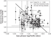 |
Fig. A.2 Same as Fig. A.1 but for the gas-phase Fe/N abundances. |
| In the text | |
|
Fig. A.3 Comparison of ratios between the observed and theoretical Hα/Hβ fluxes with the 12+log(O/H) values for a subsample of the DESIRED database with reported flux values prior to reddening corrections. |
| In the text | |
|
Fig. B.1 Upper limits to the systematic errors in the abundance of Fe2+/O+ considering a hypothetical systematic error in Te of 20%. These limits have been calculated using PyNeb (Luridiana et al. 2015) and Eq. (B.2). |
| In the text | |
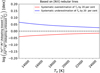 |
Fig. B.2 Same as Fig. B.1 but considering the Fe2+/N+ abundances. |
| In the text | |
|
Fig. B.3 Same as Fig. B.1 but considering the determination of the O+/H+ ionic abundances based on the [O II] λλ7319 + 7320 + 7330 + 7331 auroral lines. |
| In the text | |
|
Fig. B.4 Same as Fig. 6 but highlighting the subset of objects where the determination of the O+ abundance relies on the [O II] auroral lines. |
| In the text | |
|
Fig. B.5 Upper limits to the systematic errors in ICF(Fe) from Rodríguez & Rubin (2005) considering a hypothetical systematic error in Te of 20%. These limits have been calculated using PyNeb (Luridiana et al. 2015) and Eq. (B.2). |
| In the text | |
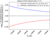 |
Fig. B.6 Same as Fig. B.5 but considering the case t2 > 0. |
| In the text | |
|
Fig. B.7 Same as Fig. B.1 but considering Fe/O=ICF × Fe2+/O+ and the propagation of their corresponding systematic errors under the case t2 = 0. |
| In the text | |
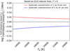 |
Fig. B.8 Same as Fig. B.7 but considering the case t2 > 0. |
| In the text | |
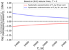 |
Fig. B.9 Same as Fig. B.7 but considering Fe/N under the case t2 = 0. |
| In the text | |
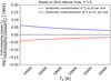 |
Fig. B.10 Same as Fig. B.9 but considering the case t2 > 0. |
| In the text | |
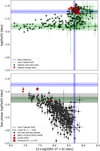 |
Fig. C.1 Same as Fig. 6 but considering an homogeneous nebular temperature t2 = 0. |
| In the text | |
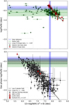 |
Fig. C.2 Same as Fig. 8 but considering an homogeneous nebular temperature t2 = 0. |
| In the text | |
Current usage metrics show cumulative count of Article Views (full-text article views including HTML views, PDF and ePub downloads, according to the available data) and Abstracts Views on Vision4Press platform.
Data correspond to usage on the plateform after 2015. The current usage metrics is available 48-96 hours after online publication and is updated daily on week days.
Initial download of the metrics may take a while.