| Issue |
A&A
Volume 689, September 2024
|
|
|---|---|---|
| Article Number | A228 | |
| Number of page(s) | 23 | |
| Section | Interstellar and circumstellar matter | |
| DOI | https://doi.org/10.1051/0004-6361/202450822 | |
| Published online | 16 September 2024 | |
MUSE spectroscopy of the high abundance discrepancy planetary nebula NGC 6153
1
Instituto de Astrofísica de Canarias,
38205
La Laguna, Tenerife,
Spain
2
Departamento de Astrofísica, Universidad de La Laguna,
38206
La Laguna, Tenerife,
Spain
3
Instituto de Astronomía (IA), Universidad Nacional Autónoma de México,
Apdo. postal 106, C.P.
22800
Ensenada, Baja California,
Mexico
4
Instituto de Ciencias Físicas, Universidad Nacional Autónoma de México,
Av. Universidad s/n,
62210
Cuernavaca, Mor.,
Mexico
5
Instituto de Física e Química, Universidade Federal de Itajubá,
Av. BPS 1303-Pinheirinho,
37500-903,
Itajubá,
Brazil
6
Nordic Optical Telescope,
Rambla José Ana Fernández Pérez 7,
38711
Breña Baja,
Spain
7
School of Physics and Astronomy, Cardiff University,
Queen’s Buildings, The Parade,
Cardiff
CF24 3AA,
UK
8
European Southern Observatory,
Karl-Schwarzschild-Str. 2,
85738
Garching bei München,
Germany
9
Gran Telescopio CANARIAS S.A.,
c/ Cuesta de San José s/n, Breña Baja,
38712
Santa Cruz de Tenerife,
Spain
Received:
22
May
2024
Accepted:
16
July
2024
Context. The abundance discrepancy problem in planetary nebulae (PNe) has long puzzled astronomers. NGC 6153, with its high abundance discrepancy factor (ADF ~ 10), provides a unique opportunity to study the chemical structure and ionisation processes within these objects.
Aims. We aim to understand the chemical structure and ionisation processes in this high-ADF nebula by constructing detailed emission line maps and examining variations in electron temperature and density. This study also explores the discrepancies between ionic abundances derived from collisional and recombination lines, shedding light on the presence of multiple plasma components.
Methods. We used the MUSE spectrograph to acquire IFU data covering the wavelength range 4600–9300 Å with a spatial sampling of 0.2 arcsec and spectral resolutions ranging from R = 1609 to R = 3506. We created emission line maps for 60 lines and two continuum regions. We developed a tailored methodology for the analysis of the data, including correction for recombination contributions to auroral lines and the contributions of different plasma phases.
Results. Our analysis confirmed the presence of a low-temperature plasma component in NGC 6153. We find that electron temperatures derived from recombination line and continuum diagnostics are significantly lower than those derived from collisionally excited line diagnostics. Ionic chemical abundance maps were constructed, considering the weight of the cold plasma phase in the H I emission. Adopting this approach we found ionic abundances that could be up to 0.2 dex lower for those derived from CELs and up to 1.1 dex higher for those derived from RLs than in the case of a homogeneous H I emission. The abundance contrast factor (ACF) between both plasma components was defined, with values, on average, 0.9 dex higher than the ADF. Different methods for calculating ionisation correction factors (ICFs), including state-of-the-art literature ICFs and machine learning techniques, yielded consistent results.
Conclusions. Our findings emphasise that accurate chemical abundance determinations in high-ADF PNe must account for multiple plasma phases. Future research should focus on expanding this methodology to a broader sample of PNe, with spectra deep enough to gather physical condition information of both plasma components, which will enhance our understanding of their chemical compositions and the underlying physical processes in these complex objects.
Key words: methods: numerical / ISM: abundances / planetary nebulae: general / planetary nebulae: individual: NGC 6153
© The Authors 2024
 Open Access article, published by EDP Sciences, under the terms of the Creative Commons Attribution License (https://creativecommons.org/licenses/by/4.0), which permits unrestricted use, distribution, and reproduction in any medium, provided the original work is properly cited.
This article is published in open access under the Subscribe to Open model. Subscribe to A&A to support open access publication.
1 Introduction
One of the unsolved questions in nebular astrophysics is whether the correct determination of the elemental abundances of elements heavier than helium in photoionised nebulae is provided by bright collisionally excited lines (CELs) or by faint recombination lines (RLs, see e.g. García-Rojas & Esteban 2007). In almost all objects studied so far, this abundance discrepancy is characterised for a given ion by the ratio of abundances obtained from RLs and CELs, which is called the abundance discrepancy factor (ADF). The ADF values are greater than 1, with a median value of about 2–3 for H II regions and the majority of planetary nebulae (PNe)1. Several scenarios have been proposed to explain this behaviour over the past decades. The most popular ones include the presence of temperature inhomogeneities in the gas (Peimbert 1967; Torres-Peimbert et al. 1980), chemical inhomogeneities in the gas (Torres-Peimbert et al. 1990; Liu et al. 2000; Tsamis & Péquignot 2005), or deviations from a Maxwellian distribution of the energy of thermal electrons (kappa distribution; Nicholls et al. 2012). Obtaining direct evidence to support any of these scenarios has proven to be a challenging task. However, observational evidence of the action of temperature fluctuations in photoionised nebulae has been found very recently, although it is restricted to H II regions (Méndez-Delgado et al. 2023).
Most of the scenarios proposed to explain the AD fail when the ADF is too high. This is the case with the increasing number of PNe exhibiting ADF values much higher than those observed in H II regions, reaching values of 10 or more. However, several studies have proposed that the presence of at least two distinct plasma components in these PNe is the driver of the high ADFs found. Although this scenario was proposed more than thirty years ago to explain the general behaviour of AD in ionised nebulae (Torres-Peimbert et al. 1990), it has only gained relevance in the last decade due to increasing observational evidence of the presence of two plasma components (e.g. Corradi et al. 2015; García-Rojas et al. 2016, 2022; Richer et al. 2022). In this scenario, one of the plasma components is very metal-rich (i.e. hydrogen-poor) and exhibits very different physical conditions compared to the main gas component that emits CELs. The origin of this metal-rich gas component is still a matter of debate, and several scenarios have been proposed, most of them linked to the fact that the majority of the high-ADF PNe appear to be associated with a close binary central star that has undergone a common envelope event (see e.g. Corradi et al. 2015; Jones et al. 2016; Wesson et al. 2018).
In this context, in order to understand the physical processes that give rise to the phenomenon of high-ADF PNe, we need to refine the abundance determinations for each of the components. The advent of the Multi Unit Spectroscopic Explorer (MUSE) integral-field spectrograph (Bacon et al. 2010) on the Very Large Telescope (VLT) has revolutionised the field of PN research, paving the way for high-spatial resolution studies that allow for detailed mapping of the physical and chemical properties on these objects. However, the first studies of the PNe NGC 7009, NGC 3132, and IC 418 (Walsh et al. 2016, 2018; Monreal-Ibero & Walsh 2020, 2022) were done using the nominal mode, which covers the wavelength range 470–930 nm that prevents the detection of the O II RLs around ~465 nm and hence, not allowing the AD problem to be addressed. In order to circumvent this issue, García-Rojas et al. (2022, hereafter GR22) obtained deep observations of three high-ADF PNe using the MUSE extended mode, which covers the wavelength range 460–930 nm, and mapping, for the first time, the spatial distribution of the O II RLs in this type of PN. GR22 emphasised the importance of taking into account the contribution of recombination to the [O II] and [N II] auroral lines, which are crucial for a proper determination of the physical conditions of the warm gas, and the relative importance of hydrogen emission in both components, which is essential to properly compute the metal content of the cold gas component, as was pointed out in the photoionisation models presented by Gómez-Llanos & Morisset (2020). Regarding this last issue, GR22 presented a methodology to compute the relative contribution of H to the H-poor gas component; however, given the lack of diagnostics to estimate the physical conditions of the H-poor gas in the three PNe studied, only rough estimates could be made in that study.
NGC 6153 is a bright, southern PN, with a relatively high ADF≃10 (Liu et al. 2000). The large amount of deep spectrophotometric data obtained for this object has made it the most studied PN in terms of the AD problem. Several observational techniques, from moderate-spectral-resolution long-slit spectroscopy scanning the entire nebular surface (Liu et al. 2000) to high-spectral-resolution échelle spectroscopy (McNabb et al. 2016; Richer et al. 2022), have been used to analyse the physical conditions and chemical abundances in this object.
Tsamis et al. (2008) attempted a 2D spectroscopic study in this PN using ARGUS/FLAMES at the VLT. The field-of-view was limited to a relatively small region of 11.5×7.2 arcsec2, covering from the central star to the south-eastern outskirts of the PN. These authors found that the ADF(O2+) computed from the abundance ratio obtained from O II λ 4649 RL and [O III] λ 4959 CEL reached values of ~20 near the PN nucleus.
Very recently, the most comprehensive and detailed spectroscopic study of NGC 6153 has been developed by Richer et al. (2022, hereafter R22). These authors took advantage of deep, high-spectral-resolution observations obtained with the UltraViolet Echelle Spectrograph (UVES) attached to UT2 of the VLT to simultaneously carry out studies of the chemical abundances and the kinematics of the gas. One of the most remarkable conclusions of the paper is the confirmation that emission from heavy-element optical RLs defines a different kinematic plasma component with a lower temperature and a higher density than the normal nebular plasma. Even more important is the fact that these authors managed to measure temperature-sensitive and density-sensitive O II and N II RLs, which allowed the computation of the physical conditions of the H-poor plasma component and, therefore, to break the degeneracies mentioned above.
In this paper we present deep MUSE spectrophotometry of the well-known PN NGC 6153 where we follow a similar approach to that of GR22 to study the spatial distribution of the physical conditions and ionic chemical abundances, taking advantage of the R22 results to refine the contribution of the different plasma components to the emissivities of the lines emitted by the nebula.
Log of the MUSE observations.
2 Observations and data reduction
NGC 6153 was observed with MUSE on the VLT, in seeing-limited mode, on the night of 6–7 July 2016. The log of the observations is provided in Table 1. The sky conditions were reasonable with a seeing of around 1 arcsec and under thin clouds. The instrument was used in its Wide Field Mode with the natural seeing (WFM-NOAO) configuration. This provides a nearly contiguous 1 arcmin2 field of view with 0.2-arcsec spatial sampling. We used the extended mode of MUSE (WFM–NOAO-E), which covers the wavelength range 460–930 nm with an effective spectral resolution that increases from R ~ 1609 at the bluest wavelengths to R ~ 3506 at the reddest wavelengths. The data are available at the ESO Science Archive under Prog. ID 097.D-0241(A) (PI: R. L. M. Corradi). Observations were obtained with dithering and a rotation of 90° between each exposure to remove artefacts during data processing. Given that the target is extended, we obtained two sky frames on each sequence (see Table 1) to perform an adequate sky subtraction. A few short exposures were also taken to analyse the strongest emission lines. The data reduction was done with esorex, using the dedicated ESO pipeline (Weilbacher et al. 2014, 2020). For each individual frame the pipeline performs bias subtraction, flat-fielding and slice-tracing, wavelength calibration, geometric corrections, illumination correction using twilight sky flats, sky subtraction (telluric absorption/emission lines and continuum) making use of the sky frames obtained between science exposures. In the final steps of the reduction process, differential atmospheric correction and flux calibration were performed.
To speed-up computations, we trimmed the original data cubes to the central 40 arcsec (200 × 200 spaxels) which is enough to cover the main nebular emission shells. In Fig. 1, we present a RGB composite image of NGC 6153 observed with MUSE, the ionisation stratification can be observed with the different colours: red for an average of [N II] λ 6548 and [S II] λ 6716, green for Hβ, and blue for He II λ 4686.
As in GR22, we checked for possible saturation of the brightest lines with a preliminary inspection of the data cubes with QFITSVIEW (Ott 2012), finding that [O III] λ 5007 and Hα lines were slightly saturated in the brightest zones. We therefore avoid using [O III] λ 5007 measurements and to minimise the effects of saturation in Hα, we followed the same procedure as in GR22 to compute the extinction coefficient.
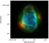 |
Fig. 1 Composite RGB image of the MUSE field of view for NGC 6153. He II λ 4686 is shown in blue, Hβ in green and an average of [N II] λ 6548 and [S II] λ 6716 in red. Intensity scale is linear. North is up, and east to the left. |
3 Emission line measurements
We constructed flux maps for 60 emission lines (30 RLs and 30 CELs). The complete list of emission lines is shown in Table C.1. All the fluxes and associated errors were measured as described in Sect. 3 of GR22. In addition, we constructed continuum maps at 8100 Å and 8400 Å, using the automated line-fitting algorithm ALFA (Wesson 2016). To only consider high signal-to-noise ratio observations, we define the following mask: F(Hβ)>0.005 × F(Hβ)max, that we apply to all emission line maps and their subsequent analysis.
In Fig. C.1, we present the unreddened fluxes of the most relevant emission lines, sorted by atomic mass and ionisation potential (IP) of the ion. The RLs of metals present a similar spatial distribution regardless of the element and IP of the emitting ion (see C II λ 6462, N II λ 5679, N III λ 46412, O I λ 7773+, and O II λ 46493), unlike the emission maps of CELs where there is a clear ionisation structure when comparing the emission of ions with different IP of the same or different element (e.g. [N I] λ 5198, [N II] λ 6548, [Ar III] λ 7136, [ArIV] λ 4740, [ArV] λ 7005). The emission line [O II] λ 7330+, which shows a morphology similar to the RLs of metals in the inner parts of the nebula, has a non-negligible recombination contribution that is estimated and subtracted from the total emission in Sec. 4.3.
We present a spatially resolved map of a neutron-capture emission line ([KrIV] at 5867.74 Å) (see Fig. C.1). To our knowledge, this emission has been previously spatially mapped only in the PN IC 2165 Otsuka (2022). The [KrIV] λ 5867.74 line emission map clearly resembles the spatial distribution of emission lines with a similar ionisation potential range, such as [O III] λ 4959.
4 Mapping the physical and chemical properties of NGC 6153
We use the v1.1.18 of PyNeb (Luridiana et al. 2015) for the emission line analysis, including 150 Monte Carlo simulations for the uncertainties estimations, following the protocol described in Sect. 3.2 of GR22. These Monte Carlo simulations allow us to generate uncertainty maps for each quantity computed in this section. In the following section, we only briefly describe the pipeline used to obtain the electron temperature and density, and the ionic abundances, and refer to GR22 for details.
4.1 Presence of a metal-rich, cold plasma phase
As already mentioned in Sec. 1, in PNe demonstrating high ADFs (greater than 10), the presence of a high-metallicity central cold phase of gas is now well established, particularly owing to the efforts made by the community in obtaining spatially resolved observations of these types of objects (Wesson et al. 2003; Corradi et al. 2015; García-Rojas et al. 2016, 2022; Richer et al. 2022). In the subsequent sections of this paper, we explain how we computed the ionic and total abundances accounting for the existence of two phases of gas: one being the “classical” warm shell emitting the CELs, and the other, more centrally emitted, metal-rich (or H-poor, with the difference lying in the He abundance; see below) and cold, as metal IR lines efficiently cool the gas. This second component serves as the primary source of the metal RLs.
Theoretical studies concerning the impact of this cold component have been published, for instance, by Péquignot et al. (2002); Yuan et al. (2011); Gómez-Llanos & Morisset (2020), and Morisset et al. (2023). In the latter paper, a theoretical framework is outlined to consider the emission emanating from each region when determining the metal abundances.
In the following sections, we will operate under the assumption that the emission lines resulting from collisional excitation originate exclusively from the warm region, while those resulting from electron recombination to a metal ion originate exclusively from the cold region. Some lines may arise from both processes (e.g. auroral lines); this will be discussed in Section 4.3.
Following the convention of Gómez-Llanos & Morisset (2020), we will adopt the acronym “ACF” for the abundance contrast factor. This is because, under the assumption of the presence of the cold region, there is no longer any abundance discrepancy, but rather two distinct components with different abundances.
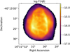 |
Fig. 2 Spatially resolved map of the Hβ measured flux (in units of erg cm−2s−1 Å−1) in logarithmic scale. |
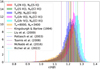 |
Fig. 3 c(Hβ) distributions obtained using different combinations of spatially resolved values of ne and Te as well as based on uniform ne = 3400 cm−3 and Te = 8000 K. Vertical lines correspond to several estimates from the literature (see text). |
4.2 Extinction correction
The observed flux map of Hβ is presented in Fig. 2, in logarithmic scale. From this bright emission line, we can distinguish the main nebular shell with two bright regions located north-west and south-east of the central star and a diffuse envelope.
The extinction correction c(Hβ) is determined with PyNeb, using the pixel by pixel median of the values obtained from Ha/Hβ, P9/Hβ, P10/Hβ, P11/Hβ, and P12/Hβ, by comparing observed values with theoretical values from Storey & Hummer (1995), and using the extinction law defined by Fitzpatrick (1999) with RV = 3.1. The theoretical line ratios have been obtained using ne = 3400 cm−3 and Te = 8000 K. These values correspond to what is found later in the process from the [Cl III] λ 5518/5538 and [S III] λ 6312/9069 line ratios, respectively (see Sec. 4.4).
Ueta & Otsuka (2021) state that for spatially resolved observations, the spatial variations in c(Hβ) cannot be recovered using a uniform (ne, Te). An iteration is performed between the spaxel-by-spaxel values of ne and Te determined later in the process, and c(Hβ), for different diagnostic line ratios. We calculate the distribution of c(Hβ) using five different combinations of spatially resolved ne and Te. In Fig. 3 we present these five c(Hβ) distributions as well as the c(Hβ) based on uniform ne = 3400 cm−3 and Te = 8000 K, and several estimates from the literature4. The c(Hβ) distributions are very consistent with each other and with the values from the literature, except for Kingsburgh & Barlow (1994) and R22, which show much lower extinctions, especially R22, whose c(Hβ) is completely outside the distributions computed here. Given the similarities of the results presented in Fig. 3 and to avoid adding noise to all emission maps, we choose to use c(Hβ) obtained from uniform values for Te and ne instead of spatially resolved maps.
The resulting map of c(Hβ) is shown in Fig. 4. We notice spatial variations in the extinction map of the order of approximately ±6% around a median value of 1.2, with a pattern similar to the spatial distribution of F(Hβ) (see Fig. 2). This indicates that part of the extinction is due to dust located inside the nebula. A similar behaviour is found for NGC 7009 (Walsh et al. 2016), where c(Hβ) roughly follows F(Hβ). These authors compute the extinction map based on MUSE observations of the same Balmer and Paschen emission line ratios, correcting Hα and Hβ from the He II Pickering lines and following an iterative process to recalculate the theoretical line ratios based on the latter estimations of Te ([S III]) and ne ([Cl III]). The variations in c(Hβ) found for NGC 7009 are much higher (more than 30%) than what we find here for NGC 6153.
The presence of the cold component described in Sec. 4.1 can affect the determination of the extinction correction because it affects the theoretical value to which the observed value is compared to obtain the correction. Anticipating the results presented in the following sections, we take both components into account using Eq. (6) from in Morisset et al. (2023) and compute the theoretical value for Hα/Hβ as being between 2.90 and 3.03, the minimum being the case of a single region at ne = 3400 cm−3 and Te = 8000 K, and the maximum corresponding to spaxels where the contribution of the cold region is maximum. These high values in the theoretical Hα/Hβ would reduce the determination of c(Hβ) from, for example, 1.2–1.14 at maximum. This would, for example, reduce the [S III] ([N II]) electron temperatures from 8300 K to 8247 K (8278 K respectively). Therefore, to avoid adding noise to the data, we do not apply any correction for the presence of the cold region.
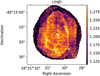 |
Fig. 4 Extinction map in logarithmic scale: c(Hβ) is obtained from the median of the extinction maps based on four Paschen lines (P9 to P12) and Hα, normalised to Hβ. |
4.3 Correction for recombination contribution
In the case of the auroral lines [N II] λ 5755 and [O II] λ 7320+30, it is well known that they are also produced by recombination, an emission process favoured at low temperatures. In the bulk of H II regions and PNe, this contribution is relatively small, and the correction is much smaller than the typical uncertainties. However, this is not the case for high-ADF PNe, where extremely strong recombination emission of both N II and O II lines from an hypothetical cold emission plasma can significantly contribute to the observed flux of these lines (see Gómez-Llanos et al. 2020). Following the procedure described in Sect. 5.2 of GR22, we correct the observed emission of [N II] λ 5755 and [O II] λ 7320+30 from the contribution due to recombination using N II λ 5679 and O II λ 4649+50 respectively by applying the following relations:
![$\[I(7320+30)_{\text {corr }}=I(7320+30)-\frac{j_{7320+30}\left(T_{\mathrm{e}}, n_{\mathrm{e}}\right)}{j_{4649+50}\left(T_{\mathrm{e}}, n_{\mathrm{e}}\right)} \times I(4649+50)\]$](/articles/aa/full_html/2024/09/aa50822-24/aa50822-24-eq1.png) (1)
(1)
![$\[I(5755)_{\text {corr }}=I(5755)-\frac{j_{5755}\left(T_{\mathrm{e}}, n_{\mathrm{e}}\right)}{j_{5679}\left(T_{\mathrm{e}}, n_{\mathrm{e}}\right)} \times I(5679),\]$](/articles/aa/full_html/2024/09/aa50822-24/aa50822-24-eq2.png) (2)
(2)
where jv(Te, Ne) are the recombination emissivities for each line.
The relation between j5755(Te, ne)/ j5679(Te, ne) and Te, for different values of ne is shown in Fig. 5. The emissivities have been obtained using PyNeb and the atomic data from Péquignot et al. (1991) and from Fang et al. (2011) for j5755 and j5679, respectively.
We explore the effect of correcting for the contribution of recombination on the determination of the temperature from the [N II] λ 5755/6548 line ratio (Eq. 2), using different values for the electron temperature of the region emitting the RLs: Te = 2000, 4000 and 6000 K, and ne = 10000 cm−3. The resulting maps, as well as the result obtained without any correction, are shown in Fig. 6. The map obtained with Te = 6000 K to calculate the recombination correction is the most uniform: we will then adopt Te = 6000 K for the correction. As explained in detail in GR22, the exact value of Te is not strictly related to the temperature of the region that emits the lines, but should rather be considered as a tuning parameter. The fact that it is not the same as the value of 2000 K obtained by R22 from O II lines may point to the uncertainties in the line emissivities in Eq. (2) and shown in Fig. 5, especially given that the ratio of emissivities is obtained by combining two different sources of atomic data. Some fluorescence mechanism may also compromise these emissivities (See Sect. 3.3 of R22). We show in Fig. 7 the effect of the correction on the auroral line emissions. Both maps on the left are not corrected, while the two maps on the right are corrected using Te = 6000 K. The central part of the nebula is the most affected by the correction (this is where the recombination contamination dominates).
Our results differ significantly from what was obtained by Liu et al. (2000) and McNabb et al. (2016). Liu et al. (2000) estimated varying recombination contributions to [N II] λ 5755 between 7 and 64%, depending on which N2+/H+ ratios were assumed, those given by far-infrared [N III] 57-μm line or by optical N II RLs, respectively. These corrections yield Te ([N II]) between 9910 K and 7110 K, which are either too high or too low when compared with the value obtained from our integrated spectra following the methodology described above (see Sect. 5.1). On the other hand, McNabb et al. (2016) estimated a very small recombination contribution to [N II] λ 5755 of only ~1%, leading to a Te ([N II]) which is ~1800 K higher than our estimate from the integrated spectrum. From the integrated spectrum of NGC 6153, we have computed a 40% recombination contribution to [N II] λ 5755 (see Sect. 5).
Regarding the recombination contribution to the [O II] λ 7320+30 lines, Liu et al. (2000) estimated that all the measured flux from these lines was due to recombination in NGC 6153. Our analysis points to different conclusions, as the flux maps of [O II] λ 7330+ and O II λ 4649+ lines shown in Fig. C.1 clearly reveal that the emission of both lines is not co-spatial. Following the described methodology, we estimated a recombination contribution of 51% to the intensity of the [O II] λ 7320+30 CELs in the integrated spectrum of NGC 6153, which seems much more reasonable given the observed emission line maps.
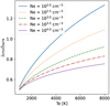 |
Fig. 5 Relationship between the emissivity due to the recombination of [N II] 5755 Å and the emissivity of N II 5679 Å. The ratios obtained for ne lower than 100 cm−3 are indiscernible. |
4.4 Physical conditions
The electron temperature and density, Te and ne, are obtained by looking for the crossing point in 2D diagnostic diagrams combining, for example, the [N II] λ 5755/6548 and the [S II] λ 6716/6731 line ratios. This is carried out with the PyNeb library and is described in more detail in GR22, including the description of the artificial neural network used to accelerate the Diagnostic.getCrossTemDen method. The atomic data used are presented in Table 2, and pre-defined in PyNeb in the ‘PYNEB_23_01’ dictionary.
The diagnostics used to derive Te and ne are listed in Table 3, grouped by the ionisation of the emitting region. In the case of the very high ionisation zone, the [Ar IV] λ 4740/4711 density diagnostic is not used due to the very noisy map of [Ar IV] λ 4711, and [Cl III] λ 5518/5538 is preferred. In Fig. 8 we show the maps corresponding to Te and ne obtained from each of these diagnostic pairs. The Te ([N II]) map has been corrected from recombination contribution as explained in Sec. 4.3.
We also obtain Te from He I RLs and Paschen jump (PJ), following the methodology described in GR22. The corresponding maps are shown in Fig. 9, as well as Te ([S III]) for comparison. It is important to emphasize that the Te maps obtained from both He I lines and PJ are heavily affected by the presence of the low temperature component (described in Sec. 4.1) with significant emission in these lines.
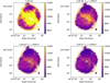 |
Fig. 6 Map of the [N II] 5755/6584 electron temperature. The upper-left panel shows the result obtained without correcting from the recombination. The following panels are showing the results obtained when the [N II] λ 5755 line is corrected for recombination using Eq. (2) and different values of the electron temperature to compute the recombination line emissivities. The value of this temperature is indicated in each panel. |
Atomic data sets used for the CELs and ORLs.
Diagnostic line ratios used to compute the electron temperature and density simultaneously.
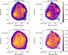 |
Fig. 7 Emission maps of the two auroral lines [N II] λ 5755 (upper panels) and [O II] λ 7330+ (lower panels), without and with correction from recombination (left and right panels, respectively). The correction is obtained using Eqs. (2) and (1), adopting Te = 6000 K and ne = 10 000 cm3. The flux is expressed in units of erg cm2s_1 Å−1 and in logarithmic scale. |
4.5 Ionic chemical abundance maps
Ionic chemical abundance maps are constructed only for the emission lines with the highest signal-to-noise ratio for each ion detected in the NGC 6153 spectrum. To determine the ionic abundances from these emission lines, we have to define the Te and ne values to be used in computing the line emissivities and the Hβ emissivity. The case of He+/H+ and He2+/H+ is relatively complicated, as there is no single plasma component emitting helium, but rather two different components: warm and cold. We will discuss them separately in Appendix A. For the RLs of heavy elements, we use the Te and ne values of 2000 K and 10 000 cm−3 obtained by R22. For the CELs, we use the Te −ne values derived from the [N II] λ 5755/6548-[S II] λ 6716/6731 for IP<17 eV, and [S III] λ 6312/9069-[Cl III] λ 5518/5538 for IP≥17 eV. Owing to the noisy maps of Te ([Ar III]) and Te ([Ar IV]) (see Fig. 8) we did not attempt to use them to compute ionic abundances; however, in Sect. 5.2 we will discuss the effect on the ionic abundances of adopting these temperatures for high ionisation potential ions (IP > 35 eV).
For the Hβ line, the usual methodology is to adopt Te and ne selected for the specific emission line (RL or CEL) in question, following the “classical” approach based on Eq. (3) from Morisset et al. (2023). A second order effect can be taken into account using a specific value for Te corresponding to the H I emission lines, as discussed by Morisset et al. (2023) at the end of their Sect. 2. In the present case, for spatially resolved maps, this value of Te (H I) would fall between Te ([N II]) and Te ([S III]). Since these two temperatures are very close, we adhere to the classical method, where Te (H I) is the same as the ionic temperature of the considered ion. Regarding the integrated spectrum, we discuss the effects of using an ad-hoc value for Te (H I) in Sect. 5.2. The abundance map of O II λ 4649.13 + 4650.85 is of particular interest as it is the one used to compute the ADF maps. However, considering the relatively low spectral resolution of the MUSE data and the results of Liu et al. (2000) and McNabb et al. (2016), these lines can be blended with C III λ 4650.25. Liu et al. (2000) reported that C III λ 4650.25 contributed ~9% to the sum of O II λ 4649.13 + 4650.85 and C III λ 4650.25 integrated fluxes. In Fig. 10, we show the oxygen abundance maps derived from O II λ 4649.13 + 4650.85 (left panel), and the lower signal-to-noise map from O II λ 4661.63 line (central panel). In the right panel of Fig. 10 we show the histograms of the O2+/H+ abundance ratio obtained from the O II λ 4649.13 + 4650.85 blend (blue) and from the O II λ 4661.63 RL (orange). It is clear that both histograms peak at very similar values but show slightly different distributions. The long tail of O II λ 4661.63 corresponds to the very high values found in the most external zones of the map, where the signal-to-noise of the line is lower. However, the differences in the distributions, evident in the left wings of both histograms, are the result of different number of spaxels with detected line emissions in each scenario. In this context, no potential contamination of the C III λ 4650.25 line can be inferred from these histograms, given the proximity of their peaks.
4.6 Weight of the cold component in the Hβ emission
As Bohigas (2015) and Morisset et al. (2023) have pointed out, for PNe with two plasma components with significantly different physical conditions, the calculation of chemical abundances must take into account the weight of the line emission in both the cold and warm components, rather than assuming homogeneous physical conditions. We have followed the methodology described by Morisset et al. (2023) to determine the chemical abundances, considering the weight of the cold region in the Hβ emission (ω, see Eqs. (5)–(8) in Morisset et al. 2023). It is worth mentioning that for the case of He ions, the case is much more complicated, since ionic He lines may be emitted by both gas phases if the cold region is not He-poor. In Appendix A we discuss such a case.
For the case of NGC 6153, the particularities of the general methodology described by Morisset et al. (2023) are the following:
The normalised Paschen jump PJ/I9229 is obtained for a grid of
![$\[T_{\mathrm{e}}^w\]$](/articles/aa/full_html/2024/09/aa50822-24/aa50822-24-eq3.png) (from 6000 to 10 000 K),
(from 6000 to 10 000 K), ![$\[T_{\mathrm{e}}^c\]$](/articles/aa/full_html/2024/09/aa50822-24/aa50822-24-eq4.png) (from 1800 to 3000 K), and ω (from 0.0 to 0.15), and constant values of
(from 1800 to 3000 K), and ω (from 0.0 to 0.15), and constant values of ![$\[n_{\mathrm{e}}^w=3000 \mathrm{~cm}^{-3}, n_{\mathrm{e}}^c=10^4 \mathrm{~cm}^{-3}, ~\mathrm{He}^{+} / \mathrm{H}^{+}=0.1\]$](/articles/aa/full_html/2024/09/aa50822-24/aa50822-24-eq5.png) , and He2+/H+ = 0.005 (Richer et al. 2022).
, and He2+/H+ = 0.005 (Richer et al. 2022).A numerical algorithm is used to interpolate the inverse problem and predict ω from:
![$\[T_{\mathrm{e}}^w, T_{\mathrm{e}}^c\]$](/articles/aa/full_html/2024/09/aa50822-24/aa50822-24-eq6.png) , and PJ/I9229.
, and PJ/I9229.From the observed map of
![$\[\mathrm{PJ} / \mathrm{I}_{9229}, T_{\mathrm{e}}^w=T_{\mathrm{e}}([\mathrm{S} ~\mathrm{\small{III}}])\]$](/articles/aa/full_html/2024/09/aa50822-24/aa50822-24-eq7.png) , and
, and ![$\[T_{\mathrm{e}}^c=2000 \mathrm{~K}\]$](/articles/aa/full_html/2024/09/aa50822-24/aa50822-24-eq8.png) , the map of ω is determined.
, the map of ω is determined.
The ionic abundances are then computed using Eqs. (7) and (8) from Morisset et al. (2023):
![$\[\left(\frac{X^i}{H^{+}}\right)^w=\frac{I_\lambda}{(1-\omega) \cdot I_\beta} \cdot \frac{\epsilon_\beta\left(T_{\mathrm{e}}^w, n_{\mathrm{e}}^w\right)}{\epsilon_\lambda\left(T_{\mathrm{e}}^w, n_{\mathrm{e}}^w\right)},\]$](/articles/aa/full_html/2024/09/aa50822-24/aa50822-24-eq9.png) (3)
(3)
for the line emitted only by the warm component (CELs) and:
![$\[\left(\frac{X^i}{H^{+}}\right)^c=\frac{I_\lambda}{\omega \cdot I_\beta} \cdot \frac{\epsilon_\beta\left(T_{\mathrm{e}}^c, n_{\mathrm{e}}^c\right)}{\epsilon_\lambda\left(T_{\mathrm{e}}^c, n_{\mathrm{e}}^c\right)},\]$](/articles/aa/full_html/2024/09/aa50822-24/aa50822-24-eq10.png) (4)
(4)
for the lines emitted only by the cold component (metal RLs).
Given that ω is obtained from the comparison between Te (PJ) and Te ([S III]) (see Eqs. (9) and (10) from Morisset et al. 2023), when both temperatures are close together, ω drops to very small values, leading to a very strong correction of the ionic abundance determined from the RLs due to the 1/ω factor in Eq. (4). These lines are actually also weakly emitted by the warm region, and Iλ is not as small as it should be if only the contribution of the cold region were considered. Here, we reach the limit of our fundamental assumption of the spatial origin of the emission lines, and the ionic abundances from RLs may be very overestimated. To avoid this effect, we cancel ω (that is, set it to Not_a_Number) when Te (PJ) reaches 85% of Te ([S III]), considering that in these spaxels the emission is mainly due to the warm region and that no correction can be determined.
In Fig. 11, we show the spatially resolved map of 1/ω and 1/(1-ω) we have obtained in NGC 6153. In order to smooth the map, we have convolved it with a 2D Gaussian kernel with σ = 2. These are the correction factors to apply to the abundances determined in the classical way (see Eqs. 3 and 4). We can see that the effect of the cold region is small on the ionic abundances determined from CELs (the factor is around 1.13), while it is very important in the case of metal RLs (a factor of 10).
In Fig. 12, we show the ionic abundance maps computed applying the parameter ω on a spaxel-by-spaxel basis.
Once we have the maps of ω and the ionic abundances, we generate the maps of the classical ADF, obtained from the ratio of abundance obtained from the RLs and CELs, computed using the abundance values without taking into account ω. We also generate maps of the same abundance ratios, but taking into account the presence of the cold region and applying ω: this is what we call the abundance contrast factor, that is, ACF (see Morisset et al. 2023). These maps are shown in Fig. 13, where the left (right) panels show the ADF (ACF) for O+/H+ (O2+/H+) in the upper (lower) panels. The effect of the cold region is clear in enhancing the contrast between both abundances by an average of ≃0.9 dex. At this point, we have to emphasize that the spatial distribution of the ADF maps is equivalent to the corresponding RL/CEL line ratios. This is an important point because the different spatial distributions of the emissivities of RLs and CELs for a given ion are not evident from Fig. C.1, contrary to the objects presented in GR22 (see their Figs. S1–S3).
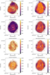 |
Fig. 8 Physical condition maps obtained using different pairs of Te−ne diagnostics. The Te ([N II]) map shown in the first row has been corrected for recombination contribution. |
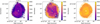 |
Fig. 9 Temperature maps obtained from He I lines (left panel), from the ratio of the Paschen jump to H I P9 (central panel), and from the [S III] λ6312/λ9069 CEL ratio (right panel). The Te scale is the same in all panels to better appreciate the differences. |
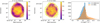 |
Fig. 10 Histogram of the oxygen abundance derived from the O II λ 4649.13 + 4650.85 RLs blend (blue) and from the O II λ 4661.63 single line (orange). |
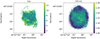 |
Fig. 11 Corrections to apply to the ionic abundances determined the classical way, for the RLs (left panel) and the CELs (right panel), see Eqs. (3) and (4). |
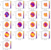 |
Fig. 12 Ionic abundances considering ω for the Hβ contribution. Metal RLs are considered to be totally emitted by the cold region (Eq. 4), while CELs are considered to be emitted by the warm region (Eq. 3). Helium ionic abundances cannot be determined from these equations, see Appendix A. |
5 The integrated emission line spectrum of NGC 6153
To compute elemental abundances of elements heavier than helium, we have to take into account unseen ionisation stages of the different elements by adopting ionisation correction factors (ICFs). GR22 pointed out that computing ICFs only makes sense when dealing with integrated spectra of the whole PN or, at least, spectra covering a significant volume of the PN that roughly includes the whole ionisation structure of the nebula. This is not the case of single spaxels of IFU observations, so elemental abundances are only computed from the integrated spectrum within the mask described in Sec. 3. We then apply the extinction correction following the same methodology presented in Sec. 4.2 to obtain the extinction-corrected line fluxes. Unreddened and extinction-corrected line fluxes along with their uncertainties are presented in Table C.1. The reported extinction-corrected line fluxes of [N II] λ 5755 and [O II] λ 7320+30 were corrected from recombination contribution assuming Te = 6000 K and ne = 10000 cm−3 (see Sec. 4.3). Lines affected by blends are also indicated in the table.
We used Monte Carlo simulations to estimate the uncertainties in the physical conditions and chemical abundances from the integrated spectrum. We generated 500 random values for each line intensity using a Gaussian distribution centred on the observed line intensity with a standard deviation σ equal to its uncertainty, then the extinction coefficient, physical conditions and chemical abundances are determined for the 501 values of line intensities, and their corresponding uncertainties are determined using standard deviation or 16–84 percentiles.
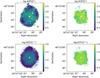 |
Fig. 13 ADF and ACF analysis: left panels show the ADF for O+ and O2+ using the traditional method. Right panels display the ACF for O+ and O2+ considering ω for the contribution of Hβ. |
Physical conditions in the integrated spectra.
5.1 Physical conditions
We computed the physical conditions (Te and ne) from the integrated spectrum using several pairs of diagnostics. As mentioned in Sec. 4.3, and following the same procedure, we have considered a 40% recombination contribution to the auroral [N II] λ 5755 line for the computation of Te ([N II]), leading to a corrected Te of 8760 K, i.e, ~1800 K lower than without taking into account such a correction. Similarly, we also applied this procedure to the intensities of the [O II] λ 7320+30 which leads to a 51% recombination contribution. In Table C.1, we present for these lines both the unreddened measured fluxes and the intensities corrected for extinction and recombination contribution.
As is well known, the main drawback of MUSE spectra of photoionised nebulae is the lack of coverage of wavelengths bluer than 4600 Å preventing the detection of the auroral [O III] λ4363 line, which is essential for computing the widely used Te ([O III]). However, the depth of the MUSE NGC 6153 spectrum allows the detection of additional Te-sensitive auroral lines in the integrated spectrum with enough signal-to-noise to compute electron temperatures. This is exemplified by the faint [Ar III] λ5192 and [Ar IV] λ7170 lines. The calculated physical conditions are presented in Table 4. To compute Te (PJ) and Te (He I) we assumed the density provided by the (Te ([S III]), ne ([S II]) pair. We also computed an averaged value of Te ([Ar III]) and Te ([Ar IV]), given by:
![$\[T_{\mathrm{e}}(\mathrm{Ar})=\theta \cdot T_{\mathrm{e}}([\mathrm{Ar} ~\mathrm{III}])+(1-\theta) \cdot T_{\mathrm{e}}([\mathrm{Ar} ~\mathrm{IV}]),\]$](/articles/aa/full_html/2024/09/aa50822-24/aa50822-24-eq11.png) (5)
(5)
where θ is the abundance ratio Ar2+/(Ar2++Ar3+). Given the ionisation potential (IP) ranges of Ar2+ (27.63–40.79 eV) and Ar3+ (40.79–59.58 eV) and the IP range of O2+ (35.12–54.94 eV), this Te diagnostic could better mimic the physical conditions in the ionisation range covered by the missing Te ([O III]) than any of the available Te diagnostics; for example, Te ([S III]) would be reliable for ions covering an IP range between 23.34–34.79 eV) and, therefore would be only representative of the mid-ionisation region in the nebula.
The electron temperature derived from the [S III] line ratio is lower than that obtained from other ions. We have used the PyNeb default set of atomic data labelled PYNEB_23_01. We made the test of modifying the default [S III] effective collision strengths from Tayal & Gupta (1999) to Grieve et al. (2014), and obtained a Te ([S III]) ≃300 K higher, which would be in better agreement with what is obtained from the [Ar III] lines. The effect of these new atomic data in the ionic abundance maps shown in Fig. 12 would be relatively small, and the resulting spatial distributions would be practically unaffected.
On the other hand, since we lack the detection of auroral [O III] lines, we rely on the average of [Ar III] and [Ar IV] temperatures, which is quite consistent with the values of Te ([O III]) derived by Richer et al. (2022, see left panel of their Fig. 37). The differences between Te ([O III]) and Te ([Ar III]), which is also consistent with our derived Te ([Ar III]), are attributed by these authors to the effect of temperature fluctuations in the warm component.
Ionic abundances (in units of 12 + log(Xi/H+)) obtained using the different recipes described in the text.
5.2 Ionic abundances
To compute the ionic abundances from the integrated spectra, we select the same set of emission lines as in the case of ionic abundance maps (see Sec. 4.5). We explore the effect of considering the weight of the cold component in the Hβ emission in the chemical abundances by applying Eqs. (3) and (4) for CELs-based and ORLs-based abundances, respectively. The contribution of recombination to the intensities of [O II] λ 7320+30 were considered following the same methodology as in Sec. 4.3.
We explore 7 different Te−ne recipes to compute ionic abundances. The first 3 recipes do not take into account ω, while recipes 4–7 use it. The description of all the recipes is available in Appendix B of the appendix. The ionic abundances obtained with these 7 recipes are given in Table 5 (as well as the temperatures adopted in each recipe).
The differences between recipes 1 to 3 in the abundances are owing to the different electron temperatures being used on each recipe. Recipes 1 and 2 are the same for the CELs; in the case of metal RLs, the small difference in ionic abundances comes from the relative differences between the corresponding metal line emissivity and the Hβ emissivity, when changing the temperatures from Te ([N II], [S III]) to 2000 K. We find a larger difference for recipe 3, where Te (PJ) was adopted to compute the Hβ emissivity. Compared to recipe 2, the abundances from CELs increase by ≃0.1 dex, while the abundances determined from RLs decrease by ≃0.35 dex. Although recipe 3 might seem reasonable, in the case of two plasma components this temperature is not representative of the emissivity of H I in either component.
The difference between recipes 1–3 and 4–7 is mainly due to the use of Eqs. (3) and (4) in the latter recipes, especially the use of ω: RL-based ionic abundances are enhanced by ≃0.9 dex, while the CEL-based ionic abundances are only enhanced by ≃0.05 dex.
In the case of recipes 4–7, RL abundances are always computed using the same temperature corresponding to the cold region. For the CEL abundances, the differences are only important for the highest excitation ions (with IP > 35 eV), as the use of higher Te than that provided by Te ([S III]), such as Te ([Ar III]) or the average of Te ([Ar III]) and Te ([ArIV]) translates into lower ionic abundances, by ≃0.1 dex or ≃ 0.25 dex, respectively.
Our favoured recipe is the number 7, where each ion emissivity (including H+) is computed using its corresponding physical conditions, and the factor ω is taken into account.
5.3 The helium case
The case of the helium ionic abundances is described in Appendix A. We apply here the same equations (A.2) and (A.3) to determine (He+/H+)w = 0.0892 and (He+/H+)c= 0.303 for the integrated spectrum.
In the case of He II we have only one line, and there is no unique solution to the single equation (A.1). The extreme values can be determined: 0 < (He2+/H+)w < 0.0120, and 0 < (He2+/H+)c < 0.073. Given that He2+ is a residual ion, the exact value of its abundance does not affect the elemental He / H ratio too much. It is nevertheless an ingredient in the determination of the ICFs used to compute the elemental abundances.
The determination of He/H for both regions is then: 0.089 < (He/H)w < 0.10, and 0.30 < (He/H)c < 0.38. The overabundance of helium in the cold region is much smaller than that of the metals. This result confirms the upper limit of He/H < 6 in the cold region, obtained by Gómez-Llanos & Morisset (2020). The emission of the dominant ion He+ that comes from each region are comparable: 60% (70%) of the He I 6678 (7281, respectively) comes from the warm phase.
5.4 Total abundances
Following our discussion in the previous section, we consider computing the total ionic abundances using a single method, taking into account ω, specifically recipe 7. This approach involves three ionisation zones, a characteristic Te for hydrogen in the warm phase, and a low Te in the cold phase, to best represent the actual values of ionic abundances.
To calculate the elemental abundances of elements heavier than helium in the warm phase, an ICF should be computed to account for unobserved ionisation states. Similarly to GR22, in this work we have taken three different approaches to calculate ICFs: i) using ICFs from the literature; ii) looking for ICFs from photoionisation models close to the observed object, and iii) computing ad hoc ICFs using machine learning techniques.
In the first approach, for N, O, S, Cl, and Ar we adopt the ICFs provided by Delgado-Inglada et al. (2014) from their equations 14, 12, 26, 29, and 35/36, respectively. Uncertainties were computed by using the analytic expressions recommended by Delgado-Inglada et al. (2014) for each case, which are based on the maximum dispersion of each ICF obtained from their grid of photoionisation models. Delgado-Inglada et al. (2015) highlighted that the calculated uncertainties in the overall abundances, based on the analytical expressions from Delgado-Inglada et al. (2014), are likely overestimated. This is because the maximum dispersion within each ICF is employed, and these ICFs have been derived from a broad grid of photoionisation models. However, real nebulae are probably more accurately depicted by a smaller selection of models. For Kr we use equation (3) by Sterling et al. (2015). To compute the final uncertainties associated with these ICFs, we consider both the uncertainties associated with the physical conditions and the ionic abundances and those related to the adopted ICF. We follow the same methodology as in Delgado-Inglada et al. (2015) and generate a uniform distribution of the ICFs with maximum and minimum values given by the uncertainties computed in Table 6, and then generate random values that we use to calculate the total abundances for 500 Monte Carlo simulations, adopting as the final errors for each abundance the 16 and 84 percentiles.
In the second method (look-up table method), we use the 3MdB_17 database (Morisset et al. 2015) to search for models that are representative of the ionisation state of NGC 6153: we select the models that are between the 5 and 95 percentiles of the following ionic abundance ratios: O2+/O+, S2+/S+, Cl3+/Cl2+ and Ar3+/Ar2+, determined from the observations using recipe 7 and 500 Monte Carlo simulations (see Sec. 5.2, and Table 5). We only search within a subset of models from 3MdB_17 under the references ref like “PNe_202_”, with com6 = 1 (realistic models, see Delgado-Inglada et al. 2014)5 and MassFrac > 0.7 (radiation- and matter-bounded models with at least 70% of the mass of the corresponding radiation-bounded model). These criteria lead to the selection of 247 models from which we determine the median, the 16%, and the 84% quantiles of the distribution of the needed ICFs.
To estimate the ad hoc ICFs from the third method, we follow the methodology described in Sect. 6.5.1 of GR22. We select a subset of photoionisation models from the 3MdB_17 database (Morisset et al. 2015) to train an Artificial Neural Network (ANN) to predict the needed ICFs from some ionic abundance ratios. In this case, we select models that fit the observed values of the O2+/O+, S2+/S+, Cl3+/Cl2+ and Ar3+/Ar2+ ionic abundance ratios within 0.5 dex, and He2+/He+ abundance ratio within 0.1 dex. We use 80% of this set of models to train the ANN (16 756 models) and test the prediction of the ANN on the remaining 20% (4189 models). The input vector is built from the five ionic abundance ratios described above. The output vector contains eight ICFs: ICF(N+/H+), ICF((O+ + O2+)/H+), ICF((S+ + S2+)/H+), ICF((Cl2+ + Cl3+)/H+), ICF((Ar2+ + Ar3+)/H+), ICF(N+/O+), ICF((S+ + S2+)/O+), and ICF(Ar2+/(O+ + O2+)). The ANN is obtained using the SciKit-Learn Python library. It contains 3 dense layers of 50, 80, and 80 RELU perceptrons, respectively. Convergence is reached using the ADAM algorithm. We consider the He+/H+ abundance for the warm region computed from Eq. (A.2) with 500 Monte Carlo simulations, and set the He2+/H+ ionic abundance as a random uniform distribution between 0 and 0.012. The exact value does not strongly affect the results. To estimate the uncertainties with this method, we compute the ICFs using the observed values of the input ionic fraction and 500 Monte Carlo simulations for He2+/He+, O2+/O+, S2+/S+, Cl3+/Cl2+ and Ar3+/Ar2+, respectively. We then determine the 16% and 84% quantiles of the distribution of the ICFs computed by the ANN.
For the cold gas component, we used only the ICFs from Delgado-Inglada et al. (2014) for C (equation (39)) and O ((equation 12)), given the lack of additional ionisation-stage diagnostics on this plasma component. In Table 6, we summarise the ICFs we obtain using the 3 methods. We do not find any systematic differences between the three methods, which provide values that are very coherent with each other.
In Table 7, we present the elemental abundances obtained from the three methods applied in this work. A comparison between the ICFs obtained using different techniques results in elemental abundances that are in relatively good agreement for all cases. It is worth mentioning that although the He2+/He fraction in each plasma component of the nebula is quite uncertain, its low value has almost no effect on the only ICF we have used from Delgado-Inglada et al. (2014), which is parameterised using this ratio (i.e. ICF(O+ + O2+)), minimising possible systematic effects on our determinations. In Fig. 14 we show the Monte Carlo distributions obtained for the elemental abundances using the ICFs shown in Table 6; only the ICF distributions obtained using more than one method are shown. The different approaches for computing the ICFs (literature, look-up table and ANN are shown in purple, green, and orange, respectively). The vertical lines on each colour show the median of the distribution.
Regarding the largest discrepancies we have found, they mostly pertain to ICFs relative to oxygen that use O+ as a proxy (i.e., ICF((N+)/O+), ICF((S+ + S2+)/O+), and ICF(Cl2+/O+)). This is because O+ is residual in this PN, and it was computed using the red [O II] λ7330+ lines, which are severely affected by recombination contribution and potentially by telluric emission. Hence, despite our careful consideration of all these effects, they could introduce systematic uncertainties to the O+/H+ ratio. However, these systematic uncertainties are mitigated in the approach we took with the look-up table and ANN methods. In contrast, in the case of nitrogen, if we use the classical ICF from Peimbert & Costero (1969), which assumes ICF(N+/O+) = 1.0, we obtain 12 + log(N/H) = 8.29, which is in slightly worse agreement with the abundances obtained using the other methods. Nonetheless, it is not entirely clear which ICF best represents this correction for PN, as a bias could be introduced in the set of photoionisation models selected by Delgado-Inglada et al. (2014) (see Delgado-Inglada et al. 2015; Amayo et al. 2020). However, The largest discrepancy is in the ICF(Ar2+/(O+ +O2+)) where it is clear that ICF of Delgado-Inglada et al. (2014) show a huge dispersion compared to the look-up table and ANN methods. This is due to the fact the Delgado-Inglada et al. (2014) method does not use Ar3+/Ar2+ as a constraint.
Ionisation correction factors (ICFs) obtained using three different methodologies (see text).
5.5 Oxygen content in the cold region
Following the method described in García-Rojas et al. (2022, see their Eqs. (5) and (6)), we compute the mass of oxygen in the form of O+ and O++ contained in the cold region, relative to that contained in the warm region. These ratios depend on the values of the electron temperature and densities in both regions, but not on ω. The results are presented in Table 8, and confirm previous results from Gómez-Llanos & Morisset (2020), R22 and GR22: the amount of oxygen in the rich and cold region is of the same order of magnitude as that embedded in the “classical” warm nebula.
Comparison between the elemental abundances determined in this work, using both the classical ICF schemes and ICFs obtained with machine-learning techniques, and those obtained in the literature.
Physical parameters and mass fraction between the warm and cold regions for O+ and O2+.
6 Discussion
6.1 Comparison with previous works
The most detailed chemical abundance studies in the literature for NGC 6153 are those by Liu et al. (2000), Tsamis et al. (2008), McNabb et al. (2016) and R22. However, not all of these authors provide elemental abundances for this PN. Tsamis et al. (2008) used IFU spectra of a portion of NGC 6153, covering from the central star to the south-eastern outskirts of the PN, and focused on computing the ADF(O2+) and on finding correlations of the ADF with different physical parameters in the PN. They did manage to compute the elemental He abundance, yielding a value of 12 + log(He/H) = 11.12. On the other hand, R22 conducted a detailed analysis of position-velocity diagrams of multiple emission lines from high-spectral resolution spectra of NGC 6153, aiming to disentangle the kinematics of the gas. Although they also computed physical conditions, ionic abundances, and ADFs as a function of gas kinematics, they did not attempt to compute elemental abundances from their integrated spectra. Finally, despite being carried out with a high-quality data set, comparisons with the results by McNabb et al. (2016) should be made with extreme caution because of their extremely low Hα/Hβ ratio (~1.0), which clearly reveals problems with data reduction.
In Table 7, we show, for comparison, the abundances reported in Liu et al. (2000) and McNabb et al. (2016). It is remarkable the excellent agreement between O abundances from CELs obtained in this work and by Liu et al. (2000). This good agreement extends, albeit to a lesser extent, to abundances of other species such as N and S (less than ~0.1 dex differences). Conversely, the differences between the abundances obtained with recombination lines are enormous, covering almost an order of magnitude in C (0.87 dex) and O (0.98 dex).
On the other hand, the agreement with the elemental abundances obtained by McNabb et al. (2016) is relatively poor, with differences ranging from 0.06 dex to 0.23 dex in abundances obtained from CELs. Particularly puzzling is the difference in the O abundance, which amounts to 0.19 dex. This difference cannot be attributed to a different temperature scheme, as we have assumed as representative for O2+, the dominant ion of this species, a Te which is only ~250 K lower than that assumed by these authors. However, we have found that the fluxes of the [O III] λλ4959,5007 lines relative to Hβ reported by these authors are between 49–51% lower than those reported in this work or in Liu et al. (2000). One could invoke differences in the excitation of the nebula in the different volumes studied as the cause of this behaviour. However, similar differences (and in the same direction) are found in the fluxes of the [O II] λ 7320+30 lines, suggesting a systematic problem with the fluxes reported by these authors that invalidates any attempt at comparison with their results.
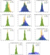 |
Fig. 14 Monte Carlo distributions of the total abundances derived from CELs with the three methods for the ICFs: literature ICFs from Delgado-Inglada et al. (2014) (purple), look-up method (green) and ANN (orange). See Table 6 for the labels of the ICFs. Vertical lines show the median of each distribution. Only ICFs obtained with more than one method are shown. |
6.2 The effect of having two different plasma components in a photoionised nebula
As outlined in Sec. 1, the hypothesis of several plasma components with significantly different physical conditions in PNe was first proposed by Torres-Peimbert et al. (1990), and since then, it has been commonly invoked as an explanation for the discrepancy found between abundances obtained from faint optical CNONe ionic RLs and the corresponding bright CELs of the same ions. However, it has only been very recently discovered that metal RLs emit from a plasma component that is clearly distinct from the CEL emission region in a small group of high-ADF PNe.
In an outstanding study using high-spectral resolution data of NGC 6153, R22 were able to disentangle a complex temperature structure in the plasma and two different kinematic components: the kinematics of most emission lines, including H and He RLs and all CELs followed a classical expansion law with outer parts of the nebula expanding faster, while heavy element RLs followed a constant expansion velocity, defining an additional plasma component. However, those authors also found, from the comparison of Te ([O III]) and Te ([ArIII]), that a contribution of relatively large temperature fluctuations in the warm component of the gas to the measured ADF cannot be ruled out (see their Sect. 4.1 and Fig. 40). This behaviour complicates the computation of the real abundances even more, especially in the warm component, as in such a case, the derived chemical abundances from CELs would be severely underestimated (see e.g. Méndez-Delgado et al. 2023).
Bohigas (2009) and Bohigas (2015) proposed studying the effect on abundance determinations of weighting the two different plasma emitting regions analytically by comparing observational data with relatively simple two-phase photoionisation models. In this paper, we explore a situation where different types of metal lines (collisional and recombination) are mainly emitted by two different regions or gas phases. This implies that the Hβ intensity, which is usually used to normalise the metal lines, needs to be distributed between the two components (this is the role of ω). The classical derivation of the ADF, defined as the ratio of line intensities and emissivities as outlined by Bohigas (2009) in its equations (1) and (2), is based on the simplification that Hβ emission is common to both sources. This is the difference between the ADF and the ACF.
Recently, a detailed photoionisation modelling of NGC 6153 was carried out by Gómez-Llanos & Morisset (2020). These authors found that a given ADF(O2+) could be reproduced by different combinations of “normal” and metal-rich components, each with different abundance contrast factors. This introduces a degeneracy in the ADF-ACF relationship, potentially causing apparently low-ADF PNe to conceal two distinct plasma components and a high ACF. Resolving this degeneracy is crucial to untangle the abundance discrepancy puzzle. Additionally, these authors stated that very high spatial and/or spectral resolution observations were the only means to isolate the contribution of the region from the total H I emission and resolve this important issue. We have made a preliminary attempt to isolate this contribution by combining our data with that of R22. However, as these previous authors wisely pointed out in their work, reality is complex. Nonetheless, we believe that our work represents a foundational step towards a deeper understanding of this type of PN. The key lies in acquiring data that facilitate reliable measurements of electron temperatures in both the cold and warm components, as well as the temperature of Hi through the Balmer and/or Paschen decrements. These are all necessary observables for computing ω and, consequently, the ACF.
The study of spatially resolved data of PNe to address the abundance discrepancy problem has been proposed in several key projects to be developed for several upcoming IFU facilities at medium- to large-sized telescopes (4–10 m). For instance, the Mirror-slicer Array for Astronomical Transients (MAAT; see Sect. 3.6 in Prada et al. 2020) is intended to be attached to the Gran Telescopio Canarias (GTC), the WEAVE Stellar, Circumstellar and Interstellar Physics survey (Jin et al. 2024, SCIP; see Sect. 4.2 in) at the 4.2 m William Herschel Telescope, and the future Wide-field Spectroscopic Telescope (Mainieri et al. 2024, WST; see Sect. 3.5.3 in) would significantly increase the amount of this type of data in the coming years. Therefore, it is necessary to establish the basis for a correct analysis and interpretation of the data, which is the aim of this work.
Based on the values presented in Table 8, we can calculate the product ne · Te, which is associated with the gas pressure. The pressure in the warm component seems to be comparable to that in the cold region (only 40% higher). Due to the uncertainties in determining the density of the cold region, we cannot definitively say if the two phases are in pressure equilibrium. This apparent lack of pressure equilibrium is common in this type of object, as the difference in density between both components is not as large as the difference in temperatures. There is at present no explanation of this fact. It is possible that the two plasma components might not be in contact because they originate from two different ejections of gas at different evolutionary times.
Finally, it is worth mentioning that very recently, observational results from high-quality observations of H II regions have revealed that the temperature fluctuations scenario applies to H II regions in the high-ionised volume of the gas (Méndez-Delgado et al. 2023). However, no evidence of such behaviour was found for PNe, although their conclusions might be affected by the small sample size, the limited metallicity range covered by the high-quality data of PNe, and the inclusion of several high-ADF PNe in the sample, which were analysed in the same way as low-ADF PNe. A more detailed analysis of an extended sample of high-quality PN spectra from the literature, with high S/N ratio detections of the weak O II RLs, as well as a careful analysis of the recombination contamination to the auroral lines, could unravel the role of possible temperature fluctuations in the observed abundance discrepancy. This sample should be free of known high-ADF PNe as well as known post-common-envelope systems harbouring a close binary central star, which could alter the conclusions of the analysis.
7 Summary
In this work, we present deep integral-field unit (IFU) spectroscopy of the high ADF (ADF ~10) PN NGC 6153. The spectra were obtained with the MUSE spectrograph covering the wavelength range 4600–9300 Å with effective spectral resolution from R = 1609 to R = 3506 for the bluest to the reddest wavelengths, respectively, and with a spatial sampling of 0.2 arcsec.
We built spatially resolved maps for 60 emission lines, as well as for two continuum regions bluer and redder to the H I Paschen discontinuity. We produced a spatially resolved map of a neutron-capture emission line, [Kr IV] λ 5867.74, which, owing to the faintness of this line, has only been attempted in one other PN.
We followed the methodology described in GR22 to perform the emission line analysis. Extinction correction is determined pixel by pixel, showing spatial variations indicative of local extinction. Accounting for a cold plasma phase could affect extinction corrections, but owing to the relatively small effect of this correction in the computed c(Hβ) and to avoid adding noise to our data, we skipped applying any correction in extinction computations for the presence of the cold region. Correction for recombination contributions to [N II] and [O II] auroral lines is performed following the methodology described in GR22. These corrections led to very different Te ([N II]) maps, highlighting the importance of accounting for multiple plasma phases in accurate nebular analyses.
The electron temperature (Te) and density (ne) from CELs were determined using the methodology described in GR22 and atomic data from Table 2. Electron temperatures were also obtained from RL diagnostics, as He I RLs and the H I Paschen jump (PJ), which are significantly lower than those obtained using CEL diagnostics, pointing to the presence of a low temperature plasma component.
Ionic chemical abundance maps were constructed using emission lines with high signal-to-noise ratios. We used a two-ionisation zone scheme to compute line emissivities. The He+/H+ and He2+/H+ ratios are determined separately for the warm and cold components, using the method described by Morisset et al. (2023).
By using the Te (o II) determined for NGC 6153 by R22 we could estimate the contribution of the cold region in the Hβ emission, and apply it to chemical abundance calculations. Maps of ω, the weight of the cold component, were generated, and correction factors were applied to the ionic abundances computed from both CELs and RLs. Maps of the abundance contrast factor (ACF) were also produced to account for the presence of the cold region. Ionic abundance maps taking into account this correction were presented.
We computed ionic abundances from the integrated spectrum of NGC,6153 following different assumptions on the Te structure and considering or ignoring the weight of the cold component in the Hβ emission. The ionic abundances obtained in this way from CELs are only slightly modified (an average of ~0.05 dex higher) with respect to a classical analysis; however, ionic abundances from RLs are nearly an order of magnitude higher.
We selected as representative for the integrated spectrum those ionic abundances computed assuming a three-zone ionisation scheme, where each ion emissivity (including H+) was computed using its corresponding physical conditions, and considering the ω factor. Ionisation correction factors (ICFs) were calculated using various methods: ICFs from the literature, look-up tables from photoionisation models, and ad hoc ICFs using machine learning techniques. In general, the three methods provide very consistent ICFs among each other. However, higher differences were found in ICFs relative to O, which use O+ as a proxy, owing to the relatively residual O+/H+ abundance in this PN and to potential systematic uncertainties in O+/H+ ratio determinations, which were derived from the red [O II] λ 7320+30 lines which are severely affected by recombination contribution and potentially affected by telluric emission. Elemental abundances in high-excitation PNe should therefore be taken with caution, especially for elements requiring a large ICF, as is the case of nitrogen.
While an observational connection between the observed abundance discrepancy and temperature fluctuations in H II regions has recently emerged, the situation regarding PNe remains enigmatic. In recent years, several studies have illustrated the presence of at least two distinct plasma components in certain PNe, often linked to short-period binary central stars that have undergone a common envelope phase. However, a comprehensive explanation for the abundance discrepancy in PNe remains elusive. We cannot definitively discard the possibility that temperature fluctuations in the warm component of the gas may partially contribute to the observed abundance discrepancy. If so, the chemical analysis of high-ADF objects would become much more complex, as ionic abundances derived from CELs may no longer be valid. Only a thorough and coherent analysis of a large sample of PN spectra covering a wide range of parameters (metallicities, excitation conditions, etc.) will shed light on this matter.
Data availability
The data products used in this paper: raw and reduced MUSE data cubes and extracted emission line maps, are available from the ESO archive facility at http://archive.eso.org/. The analysis pipeline, the emission line maps and the PYTHON scripts used for the analysis and to produce the tables and figures presented in this paper are available at https://github.com/VGomezLlanos/NGC-MUSE.
Acknowledgements
We want to dedicate this paper to the memory of our dear colleague and friend Claudio Mendoza Guardia (1951–2024) who passed away during the preparation of this paper. His contributions to atomic data computations for nebular purposes have been invaluable to the field. His insistence also made it possible for proper credit to be given to the producers of atomic data in nebular works, as it is usually done in the last years. We sincerely thank Grażyna Stasińska, the referee of this paper, for her valuable comments that enhanced its quality. This paper is based on observations made with ESO Telescopes at the Paranal Observatory under program ID 097.D-0241. VG-LL, JG-R and DJ acknowledge financial support from the Canarian Agency for Research, Innovation, and Information Society (ACIISI), of the Canary Islands Government, and the European Regional Development Fund (ERDF), under grant with reference ProID2021010074, from the Agencia Estatal de Investigación of the Ministerio de Ciencia e Innovación (AEI-MCINN) under grants “Espectroscopía de campo integral de regiones H II locales. Modelos para el estudio de regiones H II extragalaácticas” with reference DOI:10.13039/501100011033, and “Nebulosas planetarias como clave para comprender la evolución de estrellas binarias” with reference PID-2022-136653NA-I00 (DOI:10.13039/501100011033). We also acknowledge support from project P/308614 financed by funds transferred from the Spanish Ministry of Science, Innovation and Universities, charged to the General State Budgets and with funds transferred from the General Budgets of the Autonomous Community of the Canary Islands by the MCINN. JG-R also acknowledges funds from the AEI-MCINN, under Severo Ochoa Centres of Excellence Programme 2020–2023 (CEX2019-000920-S). DJ also acknowledges support from the AEI-MCINU under grant “Revolucionando el conocimiento de la evolución de estrellas poco masivas” and the European Union NextGenerationEU/PRTR with reference CNS2023-143910 (DOI:10.13039/501100011033). CM acknowledges funds from UNAM/DGAPA/PAPIIT IN 101220 and IG 101223. RW acknowledges support from STFC Consolidated grant ST/W000830/1. This work has made use of the computing facilities available at the Laboratory of Computational Astrophysics of the Universidade Federal de Itajubá (LAC-UNIFEI). The LAC-UNIFEI is maintained with grants from CAPES, CNPq and FAPEMIG.
Appendix A He+/H+ abundance maps
In this section, we discuss the case of He lines, which can be emitted by both cold and warm components. This is the general case described by Morisset et al. (2023):
![$\[\begin{aligned}& \frac{I_\lambda}{I_\beta}=\left(\frac{X^i}{H^{+}}\right)^w \cdot(1-\omega) \cdot \frac{\epsilon_\lambda\left(T_{\mathrm{e}}^w, n_{\mathrm{e}}^w\right)}{\epsilon_\beta\left(T_{\mathrm{e}}^w, n_{\mathrm{e}}^w\right)}+ \\&\quad\qquad\left(\frac{X^i}{H^{+}}\right)^c \cdot \omega \cdot \frac{\epsilon_\lambda\left(T_{\mathrm{e}}^c, n_{\mathrm{e}}^c\right)}{\epsilon_\beta\left(T_{\mathrm{e}}^c, n_{\mathrm{e}}^c\right)}.\end{aligned}\]$](/articles/aa/full_html/2024/09/aa50822-24/aa50822-24-eq51.png) (A.1)
(A.1)
Using two He I emission lines with different temperature dependencies (namely HeI 6678 Å and He I 7281 Å), we can determine the contribution of each component to the total emission and derive the ionic abundance in each component:
![$\[\left(\frac{H e^{+}}{H^{+}}\right)^w=\frac{\epsilon_\beta^w}{(1-\omega) \cdot I_\beta} \cdot \frac{I_{6678}-I_{7281} \cdot \frac{\epsilon_{6678}^c}{\epsilon_{7281}^c}}{\epsilon_{6678}^w-\epsilon_{7281}^w \cdot \frac{\epsilon_{6678}^c}{\epsilon_{7281}^c}},\]$](/articles/aa/full_html/2024/09/aa50822-24/aa50822-24-eq52.png) (A.2)
(A.2)
![$\[\left(\frac{H e^{+}}{H^{+}}\right)^c=\frac{\epsilon_\beta^c}{\omega \cdot I_\beta} \cdot \frac{I_{6678}-I_{7281} \cdot \frac{\epsilon_{6678}^w}{\epsilon_{7281}^\omega}}{\epsilon_{6678}^c-\epsilon_{7281}^c \cdot \frac{\epsilon_{6678}^w}{\epsilon_{7281}^w}},\]$](/articles/aa/full_html/2024/09/aa50822-24/aa50822-24-eq53.png)
The physical parameters for the warm (cold) component are as follows: Te = 8,300 (2,000) K, and ne =3,400 (10,000) cm−3. The ionic abundance maps for He+/H+ in each component are shown in Fig. A.1. The He+ ion is clearly more abundant in the metal-rich region, but with an enhancement of the order of 0.5 dex, smaller than the 2 dex overabundance observed for the metals.
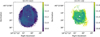 |
Fig. A.1 He+/H+ ionic abundance maps for the warm and cold region in the left and right panel, respectively. |
For the He2+ /H+ ratio, the situation is less simple since only one line of the residual He II ion is observed. We do not try to compute any value for the abundance of He2+/H+ (but see Sec 5.3 for the case of the integrated spectrum).
Appendix B Te-ne recipes to compute ionic abundances
In this section we describe the different Te-ne recipes explored in this work to compute ionic abundances.
Recipe 1: The most simple case is to adopt a general ionisation scheme with 2 zones, where [N II] λ 5755/6548-[S II] λ 6716/6731 are the physical conditions for ions with IP<17 eV, and [S III] λ 6312/9069-[ClIII] λ 5518/5538 for ions with IP≥17 eV. These conditions are used to compute the emissivities from CELs, RLs, and the Hβ line.
Recipe 2: The abundances are obtained from CELs using the same 2-IP zones as in Recipe 1. For heavy element abundances from RLs, we adopt Te = 2,000 K and ne = 10,000 cm−3 for both the line and Hβ. This is the recipe we used to generate ADF maps (left panels of Fig. 13).
-
Recipe 3: We follow a similar scheme as in Recipe 2, but we use the Paschen jump temperature to derive the Hβ emissivity in the determination of the ionic abundances, by setting the tem_HI keyword when calling the Atom.getIonAbundance method of PyNeb.
This last recipe would be the most complex one in an effort to compute the emissivities of each ion (including H+) using its corresponding temperature. But in the hypothesis of two separate plasma of very different chemical compositions, the H+ emission needs to be split into its two corresponding contributions, as in the next recipes where we take ω into account following Eqs. 3 and 4.
Recipes 4, 5 and 6: The abundances from the RLs are obtained as in Recipe 2, but multiplied by 1/ω as in Eq. 4. For the CELs, the abundances are multiplied by 1/(1 − ω) as in Eq. 3. An additional high IP zone is defined for ions with IP>35 eV. The corresponding abundances are obtained considering Te ([S III])-ne ([Cl III]), Te ([Ar IV])-ne ([Ar IV]) and the weighted average of Te ([ArIII]) and Te ([ArIV]) given by Eq. 5 with ne ([Ar IV]) for Recipes 4, 5 and 6 respectively. Indeed, recipe 4 was the one used to generate the ionic abundance maps shown in Fig. 12 and the ACF maps shown in the right panels of Fig. 13.
Recipe 7: The same scheme as in Recipe 6 is used, the only difference being the use of Te = 8,300 K for the Hβ emissivity when computing the abundances of CELs.
Appendix C Emission line flux maps and line fluxes table for the integrated spectra
In this section, we show the derredened flux maps for emission lines of 8 elements heavier than H at different ionisation stages, as well as the table with the observed and derredened fluxes of 60 emission lines in the integrated spectra of NGC 6153.
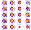 |
Fig. C.1 Flux maps of the observed emission lines of eight elements (heavier than H) in different ionisation states. The data were obtained from the MUSE datacube of NGC 6153. The flux is in units of erg cm−2s−1 Å−1 and the maps are classified by the atomic mass and the ionisation potential of the ion. We do not show here the special case of the auroral line [N II] λ 5755 which is contaminated by recombination and is discussed in more detail in Sect 4.3. |
Measured (F) and derredened (I) line fluxes in the integrated spectra.
References
- Amayo, A., Delgado-Inglada, G., & García-Rojas, J. 2020, MNRAS, 492, 950 [NASA ADS] [CrossRef] [Google Scholar]
- Bacon, R., Accardo, M., Adjali, L., et al. 2010, SPIE Conf. Ser., 7735, 773508 [Google Scholar]
- Bhatia, A. K., & Kastner, S. O. 1995, ApJS, 96, 325 [NASA ADS] [CrossRef] [Google Scholar]
- Bohigas, J. 2009, Rev. Mexicana Astron. Astrofis., 45, 107 [NASA ADS] [Google Scholar]
- Bohigas, J. 2015, MNRAS, 453, 1281 [NASA ADS] [CrossRef] [Google Scholar]
- Butler, K., & Zeippen, C. J. 1989, A&A, 208, 337 [NASA ADS] [Google Scholar]
- Corradi, R. L. M., García-Rojas, J., Jones, D., & Rodríguez-Gil, P. 2015, ApJ, 803, 99 [NASA ADS] [CrossRef] [Google Scholar]
- Davey, A. R., Storey, P. J., & Kisielius, R. 2000, A&AS, 142, 85 [NASA ADS] [CrossRef] [EDP Sciences] [Google Scholar]
- Delgado-Inglada, G., Morisset, C., & Stasińska, G. 2014, MNRAS, 440, 536 [Google Scholar]
- Delgado-Inglada, G., Rodríguez, M., Peimbert, M., Stasińska, G., & Morisset, C. 2015, MNRAS, 449, 1797 [NASA ADS] [CrossRef] [Google Scholar]
- Fang, X., Storey, P. J., & Liu, X. W. 2011, A&A, 530, A18 [NASA ADS] [CrossRef] [EDP Sciences] [Google Scholar]
- Fang, X., Storey, P. J., & Liu, X. W. 2013, A&A, 550, C2 [NASA ADS] [CrossRef] [EDP Sciences] [Google Scholar]
- Fitzpatrick, E. L. 1999, PASP, 111, 63 [Google Scholar]
- Froese Fischer, C., & Tachiev, G. 2004, Atom. Data Nucl. Data Tables, 87, 1 [NASA ADS] [CrossRef] [Google Scholar]
- Froese Fischer, C., Tachiev, G., & Irimia, A. 2006, Atom. Data Nucl. Data Tables, 92, 607 [NASA ADS] [CrossRef] [Google Scholar]
- Galavis, M. E., Mendoza, C., & Zeippen, C. J. 1995, A&AS, 111, 347 [Google Scholar]
- García-Rojas, J., & Esteban, C. 2007, ApJ, 670, 457 [CrossRef] [Google Scholar]
- García-Rojas, J., Corradi, R. L. M., Monteiro, H., et al. 2016, ApJ, 824, L27 [CrossRef] [Google Scholar]
- García-Rojas, J., Morisset, C., Jones, D., et al. 2022, MNRAS, 510, 5444 [CrossRef] [Google Scholar]
- Gómez-Llanos, V., & Morisset, C. 2020, MNRAS, 497, 3363 [CrossRef] [Google Scholar]
- Gómez-Llanos, V., Morisset, C., García-Rojas, J., et al. 2020, MNRAS, 498, L82 [CrossRef] [Google Scholar]
- Grieve, M. F. R., Ramsbottom, C. A., Hudson, C. E., & Keenan, F. P. 2014, ApJ, 780, 110 [Google Scholar]
- Jin, S., Trager, S. C., Dalton, G. B., et al. 2024, MNRAS, 530, 2688 [NASA ADS] [CrossRef] [Google Scholar]
- Jones, D., Wesson, R., García-Rojas, J., Corradi, R. L. M., & Boffin, H. M. J. 2016, MNRAS, 455, 3263 [NASA ADS] [CrossRef] [Google Scholar]
- Kaufman, V., & Sugar, J. 1986, J. Phys. Chem. Ref. Data, 15, 321 [NASA ADS] [CrossRef] [Google Scholar]
- Kingsburgh, R. L., & Barlow, M. J. 1994, MNRAS, 271, 257 [NASA ADS] [CrossRef] [Google Scholar]
- Kisielius, R., Storey, P. J., Ferland, G. J., & Keenan, F. P. 2009, MNRAS, 397, 903 [NASA ADS] [CrossRef] [Google Scholar]
- Liu, X. W., Storey, P. J., Barlow, M. J., et al. 2000, MNRAS, 312, 585 [NASA ADS] [CrossRef] [Google Scholar]
- Luridiana, V., Morisset, C., & Shaw, R. A. 2015, A&A, 573, A42 [NASA ADS] [CrossRef] [EDP Sciences] [Google Scholar]
- Mainieri, V., Anderson, R. I., Brinchmann, J., et al. 2024, arXiv e-prints [arXiv:2403.05398] [Google Scholar]
- McNabb, I. A., Fang, X., & Liu, X. W. 2016, MNRAS, 461, 2818 [NASA ADS] [CrossRef] [Google Scholar]
- Méndez-Delgado, J. E., Esteban, C., García-Rojas, J., Kreckel, K., & Peimbert, M. 2023, Nature, 618, 249 [CrossRef] [Google Scholar]
- Mendoza, C., & Zeippen, C. J. 1982, MNRAS, 199, 1025 [CrossRef] [Google Scholar]
- Monreal-Ibero, A., & Walsh, J. R. 2020, A&A, 634, A47 [NASA ADS] [CrossRef] [EDP Sciences] [Google Scholar]
- Monreal-Ibero, A., & Walsh, J. R. 2022, Galaxies, 10, 18 [NASA ADS] [CrossRef] [Google Scholar]
- Morisset, C., Delgado-Inglada, G., & Flores-Fajardo, N. 2015, Rev. Mexicana Astron. Astrofis., 51, 103 [NASA ADS] [Google Scholar]
- Morisset, C., Garcia-Rojas, J., Gomez-Llanos, V., & Monteiro, H. 2023, arXiv e-prints [arXiv:2311.14244] [Google Scholar]
- Munoz Burgos, J. M., Loch, S. D., Ballance, C. P., & Boivin, R. F. 2009, A&A, 500, 1253 [NASA ADS] [CrossRef] [EDP Sciences] [Google Scholar]
- Nicholls, D. C., Dopita, M. A., & Sutherland, R. S. 2012, ApJ, 752, 148 [NASA ADS] [CrossRef] [Google Scholar]
- Otsuka, M. 2022, MNRAS, 511, 4774 [NASA ADS] [CrossRef] [Google Scholar]
- Ott, T. 2012, QFitsView: FITS file viewer, Astrophysics Source Code Library, [record ascl:1210.019] [Google Scholar]
- Peimbert, M. 1967, ApJ, 150, 825 [NASA ADS] [CrossRef] [Google Scholar]
- Peimbert, M., & Costero, R. 1969, Bol. Observatorios Tonantzintla Tacubaya, 5, 3 [NASA ADS] [Google Scholar]
- Péquignot, D., Petitjean, P., & Boisson, C. 1991, A&A, 251, 680 [Google Scholar]
- Péquignot, D., Amara, M., Liu, X. W., et al. 2002, in Rev. Mexicana Astron. Astrofis. Conf. Series, 12, eds. W. J. Henney, J. Franco, & M. Martos, 142 [Google Scholar]
- Porter, R. L., Ferland, G. J., Storey, P. J., & Detisch, M. J. 2012, MNRAS, 425, L28 [NASA ADS] [Google Scholar]
- Porter, R. L., Ferland, G. J., Storey, P. J., & Detisch, M. J. 2013, MNRAS, 433, L89 [NASA ADS] [CrossRef] [Google Scholar]
- Pottasch, S. R., Bernard-Salas, J., Beintema, D. A., & Feibelman, W. A. 2003, A&A, 409, 599 [NASA ADS] [CrossRef] [EDP Sciences] [Google Scholar]
- Prada, F., Content, R., Goobar, A., et al. 2020, arXiv e-prints [arXiv:2007.01603] [Google Scholar]
- Ramsbottom, C. A., & Bell, K. L. 1997, Atom. Data Nucl. Data Tables, 66, 65 [NASA ADS] [CrossRef] [Google Scholar]
- Richer, M. G., Arrieta, A., Arias, L., et al. 2022, AJ, 164, 243 [NASA ADS] [CrossRef] [Google Scholar]
- Rynkun, P., Gaigalas, G., & Jönsson, P. 2019, A&A, 623, A155 [NASA ADS] [CrossRef] [EDP Sciences] [Google Scholar]
- Sterling, N. C., Porter, R. L., & Dinerstein, H. L. 2015, ApJS, 218, 25 [Google Scholar]
- Storey, P. J., & Hummer, D. G. 1995, MNRAS, 272, 41 [NASA ADS] [CrossRef] [Google Scholar]
- Storey, P. J., & Zeippen, C. J. 2000, MNRAS, 312, 813 [NASA ADS] [CrossRef] [Google Scholar]
- Storey, P. J., & Sochi, T. 2014, MNRAS, 440, 2581 [NASA ADS] [CrossRef] [Google Scholar]
- Storey, P. J., Sochi, T., & Bastin, R. 2017, MNRAS, 470, 379 [NASA ADS] [CrossRef] [Google Scholar]
- Tayal, S. S. 2011, ApJS, 195, 12 [Google Scholar]
- Tayal, S. S., & Gupta, G. P. 1999, ApJ, 526, 544 [CrossRef] [Google Scholar]
- Tayal, S. S., & Zatsarinny, O. 2010, ApJS, 188, 32 [NASA ADS] [CrossRef] [Google Scholar]
- Torres-Peimbert, S., Peimbert, M., & Daltabuit, E. 1980, ApJ, 238, 133 [NASA ADS] [CrossRef] [Google Scholar]
- Torres-Peimbert, S., Peimbert, M., & Pena, M. 1990, A&A, 233, 540 [NASA ADS] [Google Scholar]
- Tsamis, Y. G., & Péquignot, D. 2005, MNRAS, 364, 687 [NASA ADS] [CrossRef] [Google Scholar]
- Tsamis, Y. G., Barlow, M. J., Liu, X. W., Danziger, I. J., & Storey, P. J. 2003, MNRAS, 345, 186 [NASA ADS] [CrossRef] [Google Scholar]
- Tsamis, Y. G., Walsh, J. R., Péquignot, D., et al. 2008, MNRAS, 386, 22 [NASA ADS] [CrossRef] [Google Scholar]
- Ueta, T., & Otsuka, M. 2021, PASP, 133, 093002 [NASA ADS] [CrossRef] [Google Scholar]
- Walsh, J. R., Monreal-Ibero, A., Barlow, M. J., et al. 2016, A&A, 588, A106 [NASA ADS] [CrossRef] [EDP Sciences] [Google Scholar]
- Walsh, J. R., Monreal-Ibero, A., Barlow, M. J., et al. 2018, A&A, 620, A169 [NASA ADS] [CrossRef] [EDP Sciences] [Google Scholar]
- Weilbacher, P. M., Streicher, O., Urrutia, T., et al. 2014, in ASP Conf. Ser., 485, Astronomical Data Analysis Software and Systems XXIII, eds. N. Manset, & P. Forshay, 451 [Google Scholar]
- Wesson, R. 2016, MNRAS, 456, 3774 [NASA ADS] [CrossRef] [Google Scholar]
- Weilbacher, P. M., Palsa, R., Streicher, O., et al. 2020, A&A, 641, A28 [NASA ADS] [CrossRef] [EDP Sciences] [Google Scholar]
- Wesson, R., Liu, X. W., & Barlow, M. J. 2003, MNRAS, 340, 253 [NASA ADS] [CrossRef] [Google Scholar]
- Wesson, R., Jones, D., García-Rojas, J., Boffin, H. M. J., & Corradi, R. L. M. 2018, MNRAS, 480, 4589 [Google Scholar]
- Wiese, W. L., Fuhr, J. R., & Deters, T. M. 1996, Atomic Transition Probabilities of Carbon, Nitrogen, and Oxygen: A Critical Data Compilation (American Chemical Society) [Google Scholar]
- Yuan, H. B., Liu, X. W., Péquignot, D., et al. 2011, MNRAS, 411, 1035 [NASA ADS] [CrossRef] [Google Scholar]
For an updated compilation of literature values of the ADF(O2+), see https://nebulousresearch.org/adfs/
Corresponds to O II λ 4649.13 + 4650.85, and possibly affected by a blend with C III λ 4650.25. We will check the effect of this blend in chemical abundance maps in Sec. 4.5.
All Tables
Diagnostic line ratios used to compute the electron temperature and density simultaneously.
Ionic abundances (in units of 12 + log(Xi/H+)) obtained using the different recipes described in the text.
Ionisation correction factors (ICFs) obtained using three different methodologies (see text).
Comparison between the elemental abundances determined in this work, using both the classical ICF schemes and ICFs obtained with machine-learning techniques, and those obtained in the literature.
Physical parameters and mass fraction between the warm and cold regions for O+ and O2+.
All Figures
|
Fig. 1 Composite RGB image of the MUSE field of view for NGC 6153. He II λ 4686 is shown in blue, Hβ in green and an average of [N II] λ 6548 and [S II] λ 6716 in red. Intensity scale is linear. North is up, and east to the left. |
| In the text | |
|
Fig. 2 Spatially resolved map of the Hβ measured flux (in units of erg cm−2s−1 Å−1) in logarithmic scale. |
| In the text | |
|
Fig. 3 c(Hβ) distributions obtained using different combinations of spatially resolved values of ne and Te as well as based on uniform ne = 3400 cm−3 and Te = 8000 K. Vertical lines correspond to several estimates from the literature (see text). |
| In the text | |
|
Fig. 4 Extinction map in logarithmic scale: c(Hβ) is obtained from the median of the extinction maps based on four Paschen lines (P9 to P12) and Hα, normalised to Hβ. |
| In the text | |
|
Fig. 5 Relationship between the emissivity due to the recombination of [N II] 5755 Å and the emissivity of N II 5679 Å. The ratios obtained for ne lower than 100 cm−3 are indiscernible. |
| In the text | |
|
Fig. 6 Map of the [N II] 5755/6584 electron temperature. The upper-left panel shows the result obtained without correcting from the recombination. The following panels are showing the results obtained when the [N II] λ 5755 line is corrected for recombination using Eq. (2) and different values of the electron temperature to compute the recombination line emissivities. The value of this temperature is indicated in each panel. |
| In the text | |
|
Fig. 7 Emission maps of the two auroral lines [N II] λ 5755 (upper panels) and [O II] λ 7330+ (lower panels), without and with correction from recombination (left and right panels, respectively). The correction is obtained using Eqs. (2) and (1), adopting Te = 6000 K and ne = 10 000 cm3. The flux is expressed in units of erg cm2s_1 Å−1 and in logarithmic scale. |
| In the text | |
|
Fig. 8 Physical condition maps obtained using different pairs of Te−ne diagnostics. The Te ([N II]) map shown in the first row has been corrected for recombination contribution. |
| In the text | |
|
Fig. 9 Temperature maps obtained from He I lines (left panel), from the ratio of the Paschen jump to H I P9 (central panel), and from the [S III] λ6312/λ9069 CEL ratio (right panel). The Te scale is the same in all panels to better appreciate the differences. |
| In the text | |
|
Fig. 10 Histogram of the oxygen abundance derived from the O II λ 4649.13 + 4650.85 RLs blend (blue) and from the O II λ 4661.63 single line (orange). |
| In the text | |
|
Fig. 11 Corrections to apply to the ionic abundances determined the classical way, for the RLs (left panel) and the CELs (right panel), see Eqs. (3) and (4). |
| In the text | |
|
Fig. 12 Ionic abundances considering ω for the Hβ contribution. Metal RLs are considered to be totally emitted by the cold region (Eq. 4), while CELs are considered to be emitted by the warm region (Eq. 3). Helium ionic abundances cannot be determined from these equations, see Appendix A. |
| In the text | |
|
Fig. 13 ADF and ACF analysis: left panels show the ADF for O+ and O2+ using the traditional method. Right panels display the ACF for O+ and O2+ considering ω for the contribution of Hβ. |
| In the text | |
|
Fig. 14 Monte Carlo distributions of the total abundances derived from CELs with the three methods for the ICFs: literature ICFs from Delgado-Inglada et al. (2014) (purple), look-up method (green) and ANN (orange). See Table 6 for the labels of the ICFs. Vertical lines show the median of each distribution. Only ICFs obtained with more than one method are shown. |
| In the text | |
|
Fig. A.1 He+/H+ ionic abundance maps for the warm and cold region in the left and right panel, respectively. |
| In the text | |
|
Fig. C.1 Flux maps of the observed emission lines of eight elements (heavier than H) in different ionisation states. The data were obtained from the MUSE datacube of NGC 6153. The flux is in units of erg cm−2s−1 Å−1 and the maps are classified by the atomic mass and the ionisation potential of the ion. We do not show here the special case of the auroral line [N II] λ 5755 which is contaminated by recombination and is discussed in more detail in Sect 4.3. |
| In the text | |
Current usage metrics show cumulative count of Article Views (full-text article views including HTML views, PDF and ePub downloads, according to the available data) and Abstracts Views on Vision4Press platform.
Data correspond to usage on the plateform after 2015. The current usage metrics is available 48-96 hours after online publication and is updated daily on week days.
Initial download of the metrics may take a while.