| Issue |
A&A
Volume 666, October 2022
|
|
|---|---|---|
| Article Number | A115 | |
| Number of page(s) | 19 | |
| Section | Extragalactic astronomy | |
| DOI | https://doi.org/10.1051/0004-6361/202243602 | |
| Published online | 14 October 2022 | |
Measuring chemical abundances in AGN from infrared nebular lines: HII-CHI-MISTRY-IR for AGN⋆
1
Instituto de Astrofísica de Andalucía (IAA-CSIC), Glorieta de la Astronomía s/n, 18008 Granada, Spain
e-mail: This email address is being protected from spambots. You need JavaScript enabled to view it.
2
Centro de Estudios de Física del Cosmos de Aragón (CEFCA), Unidad Asociada al CSIC, Plaza San Juan 1, 44001 Teruel, Spain
Received:
21
March
2022
Accepted:
15
July
2022
Abstract
Context. Future and ongoing infrared and radio observatories such as JWST, METIS, and ALMA will increase the amount of rest-frame IR spectroscopic data for galaxies by several orders of magnitude. While studies of the chemical composition of the interstellar medium (ISM) based on optical observations have been widely spread over decades for star-forming galaxies (SFGs) and, more recently, for active galactic nuclei (AGN), similar studies need to be performed using IR data. In the case of AGN, this regime can be especially useful given that it is less affected by temperature and dust extinction, traces higher ionic species, and can also provide robust estimations of the chemical abundance ratio N/O.
Aims. We present a new tool based on a Bayesian-like methodology (HII-CHI-MISTRY-IR) to estimate chemical abundances from IR emission lines in AGN. We use a sample of 58 AGN with IR spectroscopic data retrieved from the literature, composed by 43 Seyferts, eight ultraluminous infrared galaxies (ULIRGs), four luminous infrared galaxies (LIRGs), and three low-ionization nuclear emission line regions (LINERs), to probe the validity of our method. The estimations of the chemical abundances based on IR lines in our sample are later compared with the corresponding abundances derived from the optical emission lines in the same objects.
Methods. HII-CHI-MISTRY-IR takes advantage of photoionization models, characterized by the chemical abundance ratios O/H and N/O, and the ionization parameter U, to compare their predicted emission-line fluxes with a set of observed values. Instead of matching single emission lines, the code uses some specific emission-line ratios that are sensitive to the above free parameters.
Results. We report mainly solar and also subsolar abundances for O/H in the nuclear region for our sample of AGN, whereas N/O clusters are around solar values. We find a discrepancy between the chemical abundances derived from IR and optical emission lines, the latter being higher than the former. This discrepancy, also reported by previous studies of the composition of the ISM in AGN from IR observations, is independent of the gas density or the incident radiation field to the gas, and it is likely associated with dust obscuration and/or temperature stratification within the gas nebula.
Key words: galaxies: abundances / galaxies: active / galaxies: ISM / galaxies: nuclei / infrared: ISM
Full Tables A.1–A.4 are only available at the CDS via anonymous ftp to cdsarc.u-strasbg.fr (130.79.128.5) or via http://cdsarc.u-strasbg.fr/viz-bin/cat/J/A+A/666/A115
© B. Pérez-Díaz et al. 2022
 Open Access article, published by EDP Sciences, under the terms of the Creative Commons Attribution License (https://creativecommons.org/licenses/by/4.0), which permits unrestricted use, distribution, and reproduction in any medium, provided the original work is properly cited.
This article is published in open access under the Subscribe-to-Open model. This email address is being protected from spambots. You need JavaScript enabled to view it. to support open access publication.
1. Introduction
Active galactic nuclei (AGN) are among the most luminous objects in the Universe, and can therefore be studied up to very high redshift. The interstellar medium (ISM) surrounding these nuclei is ionized by very energetic photons that are radiated from the accretion disk and jets around the supermassive black hole (SMBH). This ionization is partially reemitted in the form of strong and prominent emission lines, which can provide information on the physical and chemical properties of the region from where they originated.
Since the nebular line properties depend on the chemical composition of the ISM gas, their relative fluxes can be used to quantify the abundances of elements heavier than hydrogen and helium, known as metals (see Maiolino & Mannucci 2019 for a thorough review). While the primordial Big Bang nucleosynthesis explains the observed abundances of hydrogen or deuterium, as well as a significant fraction of helium and a small fraction of lithium (Cyburt et al. 2016), nearly all other elements are produced by stellar nucleosynthesis in the cores of stars, driven to their surfaces by convective flows and, in the late stages of their lives, are finally ejected into the ISM by stellar winds and supernovae (see review from Nomoto et al. 2013). Thus, the analysis of chemical abundances at different redshifts can provide key information on galactic evolution throughout different cosmological epochs.
The oxygen abundance (usually represented as 12+log(O/H)) is widely used as a proxy of the metal content in the ISM of galaxies, since O is the most abundant metal in mass and its presence can be easily detected through strong emission lines in the ultraviolet (UV), optical, and infrared (IR) range (Osterbrock & Ferland 2006). Another quantity relevant for analyzing the past chemical evolution of the ISM in galaxies is the nitrogen-to-oxygen abundance ratio, represented as log(N/O). This relative abundance provides essential information on the build-up of heavy elements from stellar (Chiappini et al. 2005) to galactic (Vincenzo & Kobayashi 2018) scales because it involves a primary metal, O, and another one, N, which may have a secondary origin. In the low-metallicity regime (i.e., 12+log(O/H) ≲ 8.0), N is expected to be primarily produced by massive stars, thus N/O basically a constant shows value. However, in the high-metallicity regime, N has a significant contribution from a secondary production channel, as it is formed via the CNO cycle in intermediate-mass stars, and therefore N/O tends to increase with O/H (e.g., Pérez-Montero & Contini 2009).This correlation between O/H and N/O has been determined in studies of chemical abundances in star-forming galaxies (SFGs) and HII regions in galaxies using optical observations from nearby and distant galaxies (e.g., Vila-Costas & Edmunds 1993; Pilyugin et al. 2004; Andrews & Martini 2013; Masters et al. 2016; Hayden-Pawson et al. 2022), although it has also been reported that some groups of galaxies deviate from this behavior (Amorín et al. 2010; Guseva et al. 2020; Pérez-Montero et al. 2021). Thus, the N/O determination does not only provide key information on the metal production in the ISM, but is also a necessary step in the determination of oxygen abundances when nitrogen lines are involved.
For decades, many studies have been devoted to analyzing the chemical composition of the gas-phase in SFGs using optical emission lines (e.g., McClure & van den Bergh 1968; Lequeux et al. 1979; Garnett & Shields 1987; Thuan et al. 1995; Pilyugin et al. 2004). Several techniques have been developed for that purpose: (i) the Te-method (also known as direct method), which measures the line ratios of specific collisional emission lines (CELs), sensitive to the electronic temperature and density, to directly derive the abundances of the main ionic species (e.g., Aller 1984; Osterbrock & Ferland 2006); (ii) by means of photoionization models to reproduce the observed CELs and then constrain chemical and physical properties of the region, using several codes such as CLOUDY (Ferland et al. 2017), MAPPINGS (Sutherland & Dopita 2017), or SUMA (Contini & Viegas 2001); and (iii) the use of empirical or semiempirical calibrations between accurate chemical abundances and the relative fluxes of strong emission lines (e.g., Pérez-Montero & Contini 2009; Pilyugin & Grebel 2016; Curti et al. 2017). Furthermore, new approaches take advantage of more than one of the above techniques at the same time, such as HII-CHI-MISTRY (hereinafter HCM, Pérez-Montero 2014), which uses sensitive ratios to chemical abundances to search for the best fit among a grid of photoionization models.
In recent years, the analysis of chemical abundances in the gas-phase of HII regions has been extended to the narrow line region (NLR) in AGN (e.g., Storchi-Bergmann et al. 1998; Contini & Viegas 2001; Dors et al. 2015; Pérez-Montero et al. 2019; Thomas et al. 2019; Flury & Moran 2020; Pérez-Díaz et al. 2021). This region of the ISM, located between ∼102 pc and a few kpc (Bennert et al. 2006a,b), is characterized by an electronic density, ne, typically in the 102–104 cm−3 range, and an electronic temperature of Te ∼ 104 K (Vaona et al. 2012; Netzer 2015). Although these physical conditions may not depart significantly from to those of the ISM in HII regions (Osterbrock & Ferland 2006), the source and the shape of the ionizing continuum are completely different in both cases: the accretion disk in AGN, which produces a power-law-like continuum extending to high energies; and a thermal-like continuum from massive O- and B-type stars in HII regions. This difference has profound effects on the emission-line spectrum, as some highly ionized species are not found in HII regions, while their contribution is not negligible in AGN due to the harder radiation fields involved (Kewley et al. 2019; Flury & Moran 2020). Thus, the techniques developed for the metal content study in SFGs must take these differences into account when applied to the AGN case (e.g., Dors et al. 2015; Pérez-Montero et al. 2019; Carvalho et al. 2020; Flury & Moran 2020; Pérez-Díaz et al. 2021).
Chemical abundances can also be derived using emission lines in the UV range. This is the case for galaxies at redshift z ≳ 1–2, where UV lines can be measured by optical telescopes, allowing the determination of chemical abundances in SFGs (e.g., Erb et al. 2010; Dors et al. 2014; Berg et al. 2016; Pérez-Montero & Amorín 2017) and in AGN (Dors et al. 2019). In these cases, besides the oxygen abundance 12+log(O/H), it is also important to constrain the carbon-to-oxygen ratio log(C/O), since C emits strong UV emission lines that are easily detected and, as N, it is also a metal with both primary and secondary origins.
Nevertheless, the determination of chemical abundances using optical and, above all, UV emission lines, can be seriously affected by reddening. In particular, deeply dust-embedded regions may go unnoticed by optical and UV tracers, which therefore will not be able to probe their content of heavy elements. In addition, the optical and UV CELs present a non-negligible dependence on some physical properties of the ISM, such as the electronic temperature (Te) or the electronic density (ne), which are difficult to take into consideration, either in empirical calibrations or in models. These problems do not arise when chemical abundances are derived from IR emission lines. The relative insensitivity of IR lines to interstellar reddening allows us to peer through the dusty regions in galaxies (Nagao et al. 2011; Pereira-Santaella et al. 2017; Fernández-Ontiveros et al. 2021). In addition, the negligible dependence of the IR line emissivity on Te (see Fig. 1 in Fernández-Ontiveros et al. 2021) avoids the large uncertainties in the temperature determination that affects the abundances based on optical lines. For instance, Dors et al. (2013) suggest that extinction effects and temperature fluctuations might be an explanation for the discrepancy between optical and infrared estimations of the neon abundances. Temperature fluctuations have also been reported in previous works, for example, Croxall et al. (2013) analyzing a sample of HII regions in NGC 628 used fine-structure IR and also optical emission lines. An example of the effect of dust obscuration can be found in Fernández-Ontiveros et al. (2021), where they estimate twice the metallicity of NGC 3198 from IR emission lines when comparing with their optical estimations.
In recent decades, several IR spectroscopic telescopes, such as the Infrared Space Observatory (ISO, covering the 2.4–197 μm range, Kessler et al. 1996), the Spitzer Space Observatory (5–39 μm, Werner et al. 2004), the Herschel Space Observatory (51–671 μm, Pilbratt et al. 2010) and the Stratospheric Observatory for Infrared Astronomy (SOFIA, covering the 50–205 μm range, Fischer et al. 2018), have provided essential information of these emission lines for a considerable amount of sources. Moreover, upcoming missions such as the James Webb Space Telescope (JWST, which will cover the 4.9–28.9 μm range with the Mid-InfraRed Instrument MIRI, Rieke et al. 2015; Wright et al. 2015) and the Mid-infrared ELT Imager and Spectograph (METIS, covering the N-band centered at 10 μm, Brandl et al. 2021) will increase the amount of information from IR observations of local galaxies, significantly improving recent studies of chemical abundances based on IR emission lines (Peng et al. 2021; Fernández-Ontiveros et al. 2021; Spinoglio et al. 2022) and laying the foundations to extend the analyses to higher redshifts (z > 4) with the Atacama Large Millimeter/submillimeter Array (ALMA; Wootten & Thompson 2009).
In this work we present an IR version of the method HCM developed by Pérez-Montero (2014) to derive chemical abundances from optical emission lines in SFGs, and later extended to the NLR region of AGN by Pérez-Montero et al. (2019; hereinafter denoted as PM19). This version of HII-CHI-MISTRY-IR, or HCM-IR, complements the work done by Fernández-Ontiveros et al. (2021; hereinafter denoted as FO21) for SFGs. By taking advantage of a grid of photoionization models covering a wide range in 12+log(O/H), log(N/O), and log(U), our method computes these three parameters by fitting emission-line ratios that are sensitive to those quantities.
The work is organized as follows. In Sect. 2 we describe a sample of galaxies with available spectroscopic IR data used to check the method. This sample is composed of Seyferts, ULIRGs, LIRGs and LINERs, which show Ne4+ emission lines characteristic of AGN activity (Genzel et al. 1998; Pérez-Torres et al. 2021). In Sect. 3 we describe the methodology underlying HCM-IR, including the emission-line ratios used to estimate chemical abundances and the differences with those proposed by FO21 when applied to the AGN case. In Sect. 4 we present the main results from HCM-IR for our sample of galaxies, also comparing them with estimations from optical observations. In Sect. 5 we present a full discussion on these results and we summarize in Sect. 6 the main conclusions from this work.
2. Sample
To probe the validity of the diagnostics detailed in Sect. 3, we compiled a sample of 58 AGN with spectroscopic observations in the mid- and far-IR ranges from Spitzer/IRS (Werner et al. 2004; Houck et al. 2004) and Herschel/PACS (Pilbratt et al. 2010; Poglitsch et al. 2010), respectively. Most of the galaxies (48) were drawn from the IR spectroscopic atlas in Fernández-Ontiveros et al. (2016), corresponding to the objects with a detection of a hydrogen recombination line in the IR range, namely Brackett-α at 4.05 μm (Brα), Pfund-α at 7.46 μm (Pfα), or Humphreys-α at 12.4 μm (Huα). The sample was completed with nine galaxies with available additional SOFIA/FIFI-LS observations (Temi et al. 2014; Fischer et al. 2018) of the [NIII]57 μm and/or the [OIII]52, 88 μm lines from Spinoglio et al. (2022). Thus, the sample selection maximizes the number of AGN galaxies with detections of these lines, which allows us to obtain N/O abundance ratios that are independently derived from the oxygen abundance.
The Brα and Pfα line fluxes were collected from the literature, while new measurements of the Huα line for 11 galaxies are presented in this work (see Table A.1). The latter were obtained from the calibrated and extracted Spitzer/IRS high-resolution spectra (R = 600) in the CASSIS database (Lebouteiller et al. 2015). The line flux was measured by direct integration of the spectrum at the rest-frame wavelength of the line, subtracting the continuum level derived from a linear polynomial fit to the adjacent continuum on both sides of the line.
The final sample thus consists of 17 Seyfert 1 nuclei (Sy1), 14 Seyfert nuclei with hidden broad lines in the polarized spectrum (Sy1h), 12 Seyfert 2 nuclei (Sy2), three LINERs, four LIRGs and eight ULIRGs.
We present in Fig. 1 a classification of our sample of AGN based on the so-called BPT-IR1 diagram (Fernández-Ontiveros et al. 2016). In contrast with the optical diagnostic diagrams (Baldwin et al. 1981; Kauffmann et al. 2003; Kewley et al. 2006), the axes on the BPT-IR diagram represent ratios of the different ionized states for the same element, in other words, they do not show any dependence on the chemical abundances. Although pure AGN models (blue) do not cover the region where ULIRGs, LIRGs, and LINERs fall, a significant amount of our Seyfert sample are in agreement with AGN-dominated models. We also represent the same models from Fernández-Ontiveros et al. (2016) for dwarf galaxies and SFGs, and we find that they do not cover the region where our sample of AGN is located, implying that part of our sample shows both star-formation and AGN activity. Nevertheless, the detection of Ne4+ IR lines in these galaxies supports the idea that AGN activity dominates our sample (Genzel et al. 1998; Armus et al. 2007; Izotov et al. 2012; Pérez-Torres et al. 2021).
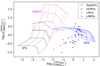 |
Fig. 1. BPT or diagnostic diagram in the IR range, proposed to distinguish between spectral types (Fernández-Ontiveros et al. 2016). Models computed with CLOUDY v17.02 (Ferland et al. 2017) are presented as lines: black for SFG models computed from the library STARBUST99 (González Delgado & Leitherer 1999) with 12+log(O/H) = 8.69 and log(N/O) = −0.86; magenta for dwarf models computed from a starburst of ∼106 yr with 12+log(O/H) = 8.0 and log(N/O) = −0.86; and blue for AGN models computed from the same SED used in this work (αOX = −0.8 and αUV = −1.0, see Sect. 3) with 12+log(O/H) = 8.69 and log(N/O) = −1.0. For all models, dotted lines trace models with the same electronic density (ranging 10–107 cm−3), while dashed lines represent fixed values of the ionization parameter U. |
3. Photoionization models and abundance estimations
Chemical abundances (O/H and N/O) and the ionization parameter (U) were derived using an updated version of the Python code HII-CHI-MISTRY-IR2 (FO21) from IR emission lines, adapting it to work for AGN by using the same models used for the optical version of the code, and described in PM19. We denote the optical version as HCM, while its infrared version presented here will be denoted as HCM-IR. We follow the methodology used by FO21, taking into account some differences that arise when considering AGN instead of SFG models.
3.1. Grids of AGN photoionization models
HCM-IR estimates chemical abundances (O/H and N/O) and U using a Bayesian-like calculation, by comparing certain observed IR emission-line flux ratios with the corresponding values as predicted by large grids of photoionization models. The models were computed using CLOUDY v17 (Ferland et al. 2017) and they are the same as those employed by PM19. In these models, the gas phase is characterized by an electronic density of ne = 500 cm−3. All models assume a standard dust-to-gas mass ratio and the gas-phase abundances were scaled in each model to O following the solar photospheric proportions reported by Asplund et al. (2009), with the exception of N, which is considered as a free parameter in the grids for an independent estimation of the N/O ratio. The source of ionization is an AGN spectral energy distribution (SED) composed by a Big Blue Bump peaking at 1 Ryd and a power law for X-ray nonthermal emission characterized by αX = −1.0. The continuum between UV and X-ray ranges is represented by a power law with an index of αOX = −0.8 or αOX = −1.2. The filling factor was set to 0.1 while two stopping criteria were considered: a fraction of free electrons of 2% or 98%. Thus, a total of four grids of photoionization models (i.e., assuming two different values for αOX and two different stopping criteria) can be considered and selected by the user in an iterative process while running HCM-IR. Hereafter, we discuss the grid of models corresponding to αOX = −0.8 and a stopping criteria of 2% of free electrons. The effects of using different grids will be discussed in Sect. 3.5.
The grids cover a range from 12+log(O/H) = 6.9 to 9.1 in steps of 0.1 dex, a range from log(N/O) = −2.0 to 0.0 in steps of 0.125 dex, and a range from log(U) = −4.0 to −0.5 in steps of 0.25 dex. The behavior of some of the emission-line ratios used by the code shows a bivaluation in the [−4.0, −2.5] and [−2.5, −0.5] ranges. This behavior for some optical emission-line ratios was also discussed in PM19 and reported by Pérez-Díaz et al. (2021). For this reason, the grids are constrained to certain U ranges by considering two branches: the low-ionization branch, which covers the [−4.0, −2.5) range, and the high-ionization branch, covering [−2.5, −0.5].
The code takes as input the following IR emission lines: H Iλ4.05 μm, H Iλ7.46 μm, [S IV]λ10.5 μm, H Iλ12.4 μm, [Ne II]λ12.8 μm, [Ne V]λ14.3 μm, [Ne III]λ15.6 μm, [S III]λ18 μm, [Ne V]λ24 μm, [O IV]λ26 μm, [S III]λ33 μm, [O III]λ52 μm, [N II]λ57μm, [O III]λ88 μm, [N II]λ122 μm, and [N II]λ205 μm, which can be introduced in arbitrary units and are not necessarily reddening-corrected. Since our AGN models consider a higher electronic density than SFG models used by FO21 (AGN models assume ne = 500 cm−3 while SFG models assumed ne = 100 cm−3), special attention must be paid to the critical density of the emission lines, which are much lower than those that characterize optical emission lines (e.g., Osterbrock & Ferland 2006). Considering different electronic temperatures Te characteristic of the ionic species in our models, we summarized in see Table 1 the critical densities for all emission lines used as inputs with PYNEB (Luridiana et al. 2015). Therefore, from the set of lines used by HCM-IR for SFG models (FO21), we omitted three of them due to their relatively low critical densities when compared to the electronic density adopted for the models [N II]λ205 μm, [N II]λ122 μm, and [O III]λ88 μm. The code only takes into account [O III]λ88 μm when [O III]λ52 μm is missing, although we warn that observed emission lines may deviate from predictions due to contributions of diffuse ionized gas (DIG), leading to uncertainties in the estimated chemical abundances.
Computed critical densities (cm−3) for fine structure IR lines from PYNEB, for different electronic temperatures.
In addition, we omitted the emission line [S III]λ33 μm, which is an input for the SFG version of the code. Despite being stronger than [S III]λ18 μm, the introduction of this emission line in the calculations of the code leads to wrong estimations of both O/H and U (see Sect. 3.4 for more details). Also, in contrast with the input used for SFGs, we consider [Ne V] emission lines, which are preferentially detected in infrared observations of galaxies hosting AGN (Genzel et al. 1998; Armus et al. 2007; Izotov et al. 2012; Pérez-Torres et al. 2021), and the [O IV] emission line, characteristic of AGN activity (Meléndez et al. 2008; Rigby et al. 2009; LaMassa et al. 2010) since it can only be marginally produced in extremely highly ionized (log(U) ≳ −1.5) star-forming regions.
Instead of matching single emission lines to predicted observations, HCM-IR uses particular emission-line ratios (listed below) to match observations and predictions. Then, the abundances O/H, N/O, and U are calculated following a χ2 methodology, being the mean of all input values of the models weighted by the quadratic sum of the differences between observations and predictions, which is the same methodology described in PM19. After the first iteration, N/O is fixed and the grid of models is constrained. Then, O/H and U values are calculated in later iterations considering the already constrained model grids. When errors on the emission-line fluxes are provided, the code also takes them into account in the final uncertainty of the estimations with a Monte Carlo simulation by perturbing the nominal input emission-line fluxes in the range delimited by their corresponding error.
3.2. N/O estimation
To estimate N/O, HCM-IR considers two emission-line ratios. The first one is N3O3, proposed by several authors (e.g., Nagao et al. 2011; Pereira-Santaella et al. 2017; Peng et al. 2021; Fernández-Ontiveros et al. 2021), which is an infrared analog of the estimator N2O2 usually used in the optical range due to its effectiveness for both AGN and SFGs (Pérez-Montero et al. 2019) to derive the same abundance ratio (e.g., Pérez-Montero & Contini 2009). The N3O3 is defined as:
![Mathematical equation: $$ \begin{aligned} \log \left( \mathrm{N3O3} \right) = \log \left( \frac{ \mathrm{I} \left( \left[ {\text{N}}{\small {{\text{ III}}}} \right] _{57\,\upmu \mathrm{m}} \right) }{ \mathrm{I} \left( \left[ {\text{O}}{\small {{\text{ III}}}} \right] _{52\,\upmu \mathrm{m}} \right) } \right). \end{aligned} $$](/articles/aa/full_html/2022/10/aa43602-22/aa43602-22-eq1.gif) (1)
(1)
Our definition of N3O3 only takes into account [O III]λ52 μm because the other [O III] IR emission line presents a critical density close to the electronic density of our models, in contrast to the same estimator defined for star-forming regions as described by FO21, which also takes into account [O III]λ88 μm. When [O III]λ52 μm is not provided, the code calculates N3O3 using [O III]λ88 μm. This modification is only taken into account when the code is applied for AGN, but not in the case of SFGs since the grid of models for those cases is calculated for ne ∼ 100 cm−3 (FO21). As for its optical analog, this estimator has little dependence on U as shown in Fig. 2a. Moreover, our grid of AGN models and the grid of SFGs show that this parameter is almost independent of the spectral type, meaning there is little distinction between AGN and SFG models.
The second emission-line ratio used by the code to derive N/O is N3S34, which takes advantage on the primary origin of sulfur (as in the case of oxygen), is defined as:
![Mathematical equation: $$ \begin{aligned} \log \left( \mathrm{N3S34} \right) = \log \left( \frac{ \mathrm{I} \left( \left[ {\text{N}}{\small {{\text{ III}}}} \right] _{57\,\upmu \mathrm{m}} \right) }{ \mathrm{I} \left( \left[ {\text{S}}{\small {{\text{ III}}}} \right] _{18\,\upmu \mathrm{m}} \right) + \mathrm{I} \left( \left[ {\text{S}}{\small {{\text{ IV}}}} \right] _{10\,\upmu \mathrm{m}} \right) } \right). \end{aligned} $$](/articles/aa/full_html/2022/10/aa43602-22/aa43602-22-eq2.gif) (2)
(2)
This ratio also correlates with N/O, presenting little dependence on O/H, as shown in Fig. 2b. Moreover, this tracer also presents a tight correlation with N/O when SFG models are considered. Thus, we have also added this estimator in the calculations of HCM-IR for SFGs, with the particular difference that emission line [S III]λ33 μm is also considered for SFGs.
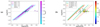 |
Fig. 2. Relations between different IR emission-line ratios with N/O. (a) Relation with N3O3 in our sample. The colorbar shows estimations of log(U). AGN models for a fixed value of 12+log(O/H) = 8.6 are presented as continuous lines, while dashed lines correspond to SFG models for the same fixed value. (b) Relation with the N3S34 estimator in our sample. The colorbar shows estimations of 12+log(O/H). AGN models for a fixed value of log(U) = −2.0 are presented as continuous lines, while dashed lines correspond to SFG models for the same fixed value. For both plots, blank points indicate that no estimation can be provided of the colored quantity. The following spectral types are represented: Seyferts 2 as circles; ULIRGs as squares; LIRGs as triangles; and LINERs as stars. |
Considering the behavior of the AGN models in both Figs. 2a and b, we obtain the following linear calibrations using data from the photoionization models:
 (3)
(3)
 (4)
(4)
which can be used as alternative to the code to directly estimate N/O.
3.3. O/H and U estimations
Once N/O has been determined in a first iteration, as this involves emission-line ratios with little dependence on other input parameters, the code estimates in a second iteration both O/H and U from a subgrid of models compatible with the previous estimation of N/O. Therefore, this guarantees that no previous assumption between O/H and N/O is introduced. In case N/O cannot be constrained due to the lack of key emission lines, a relation between O/H and N/O is assumed by the code. By default, this relation is the one obtained by Pérez-Montero (2014) for star-forming regions using chemical abundances based on optical emission-lines. However, this relation can be modified by any user of the code adopting alternative laws within the corresponding libraries.
To estimate O/H and U, the code uses multiple emission-line ratios that are sensitive to the above quantities. One of them is based on neon lines and comes from a modification of the estimator Ne23 proposed by Kewley et al. (2019) and FO21 to account for [Ne V] lines that are more prominent in AGN than in SFGs. Then, accordingly, the estimator Ne235 for O/H can be defined as:
![Mathematical equation: $$ \begin{aligned} \log \left( \mathrm{Ne235} \right)&= \log \left( \frac{ \mathrm{I} \left( \left[ {{\text{ Ne}}{\small {{\text{ II}}}}} \right] _{12\upmu \mathrm{m}} \right) + \mathrm{I} \left( \left[ {{\text{ Ne}}{\small { {\text{ III}}}}} \right] _{15\,\upmu \mathrm{m}} \right) }{ \mathrm{I} \left( {{\text{ H}}{\small {{\text{ I}}}}} _{i} \right) } \right. \nonumber \\&\quad + \left. \frac{ \left[ \mathrm{I} \left( {{\text{ Ne}}{\small {{\text{ V}}}}} \right] _{14\,\upmu \mathrm{m}} \right) + \mathrm{I} \left( \left[ {{\text{ Ne}}{\small {{\text{ V}}}}} \right] _{24\,\upmu \mathrm{m}} \right) }{ \mathrm{I} \left( {{\text{ H}}{\small {{\text{ I}}}}} _{i} \right) } \right), \end{aligned} $$](/articles/aa/full_html/2022/10/aa43602-22/aa43602-22-eq5.gif) (5)
(5)
with H Ii being one of the hydrogen lines that the code can take as input. In cases where more than one of the hydrogen lines are introduced as input, HCM-IR calculates Ne235 for each hydrogen line, taking all considered ratios in the resulting weighted-distribution. In addition, these same neon lines are used to estimate log(U) from the ratio Ne23Ne5, defined as:
![Mathematical equation: $$ \begin{aligned} \log \left( \mathrm{Ne23Ne5} \right) = \log \left( \frac{ \mathrm{I} \left( \left[ {\text{Ne}}{\small {{\text{ II}}}} \right] _{12\,\upmu \mathrm{m}} \right) + \mathrm{I} \left( \left[ {\text{Ne}}{\small { {\text{ III}}}} \right] _{15\,\upmu \mathrm{m}} \right) }{ \mathrm{I} \left( \left[ {\text{Ne}}{\small { {\text{ V}}}} \right] _{14\,\upmu \mathrm{m}} \right) + \left[ \mathrm{I} \left( {\text{Ne}}{\small { {\text{ V}}}} \right] _{24\,\upmu \mathrm{m}} \right) } \right), \end{aligned} $$](/articles/aa/full_html/2022/10/aa43602-22/aa43602-22-eq6.gif) (6)
(6)
which is a modification of the estimator Ne2Ne3 proposed by several authors (Thornley et al. 2000; Yeh & Matzner 2012; Kewley et al. 2019; FO21) to account for the high-ionic species of Ne, which are found in AGN. Figure 3a shows the behavior of Ne235 with 12+log(O/H). There is little dependence on U and there is clear separation between SFG and AGN models, which is explained by the little capacity of SFG models to produce [Ne V]. Figure 3b shows the relation between Ne23Ne5 and log(U). The behavior of the models, well reproduced by the estimations in our sample, clearly shows the bi-valuation that forces the code to distinguish between low- and high-ionization AGN. For low-ionization AGN models, little dependence is found on O/H, while it has a more significant impact on the upper branch (i.e., high-ionization AGN models). The lack of SFG models in this figure justifies the omission of [Ne V] lines in SFG estimators.
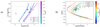 |
Fig. 3. Relations of different ratios involving Ne IR emission-lines with O/H and log(U). (a) Relation between the Ne235 estimator, using H I 4 μm, and 12+ log(O/H) in our sample. The colorbar shows estimations of log(U). (b) Relation between estimator Ne23Ne5 and log(U) in our sample. The colorbar shows estimations of 12+log(O/H). For both plots, blank points indicate that no estimation can be provided of the colored quantity. AGN models for a fixed value of log(N/O) = −1.0 are presented as continuous lines, while dashed lines correspond to SFG models for the same fixed value. The following spectral types are represented: Seyferts 2 as circles; ULIRGs as squares; LIRGs as triangles; and LINERs as stars. |
Another set of IR emission lines that HCM-IR uses to estimate O/H and U are the sulfur lines. To calculate both quantities, the code uses the estimators S34 (FO21) and S3S4 (Yeh & Matzner 2012; FO21) respectively, defined as:
![Mathematical equation: $$ \begin{aligned} \log \left( \mathrm{S34} \right)&= \log \left( \frac{ \mathrm{I} \left( \left[ {\text{S}}{\small { {\text{ III}}}} \right] _{18\,\upmu \mathrm{m}} \right) + \mathrm{I} \left( \left[ {\text{S}}{\small { {\text{ IV}}}} \right] _{10\,\upmu \mathrm{m}} \right) }{ \mathrm{I} \left( {\text{H}}{\small { {\text{ I}}}} _{i} \right) } \right),\end{aligned} $$](/articles/aa/full_html/2022/10/aa43602-22/aa43602-22-eq7.gif) (7)
(7)
![Mathematical equation: $$ \begin{aligned} \log \left( \mathrm{S3S4} \right)&= \log \left( \frac{ \mathrm{I} \left( \left[ {\text{S}}{\small { {\text{ III}}}} \right] _{18\,\upmu \mathrm{m}} \right) }{ \mathrm{I} \left( \left[ {\text{S}}{\small { {\text{ IV}}}} \right] _{10\,\upmu \mathrm{m}} \right) } \right). \end{aligned} $$](/articles/aa/full_html/2022/10/aa43602-22/aa43602-22-eq8.gif) (8)
(8)
Our definitions of these two estimators differ from those used in FO21 since we omit [S III]λ33 μm in our calculations. Figure 4a shows that S34 correlates with 12+log(O/H) and has also little dependence on U, although in this case there is no clear separation between SFG and AGN models. Figure 4b reinforces our preliminary statement about the need to distinguish between low- and high-ionization AGN due the bi-valuation of log(U) with S3S4. We also observed that for low-ionization parameters (log(U) < −2.5), the behavior of AGN and SFG models is similar, although they cover different regions of the diagram.
In the same fashion that we proceed with the sulfur lines, the code takes into account estimators based on IR oxygen lines. We define O34 and O3O4 to estimate 12+log(O/H) and log(U) respectively as:
![Mathematical equation: $$ \begin{aligned} \log \left( \mathrm{O34} \right)&= \log \left( \frac{ \mathrm{I} \left( \left[ {\text{O}}{\small { {\text{ III}}}} \right] _{52\,\upmu \mathrm{m}} \right) + \mathrm{I} \left( \left[ {\text{O}}{\small { {\text{ IV}}}} \right] _{26\,\upmu \mathrm{m}} \right) }{ \mathrm{I} \left( {\text{H}}{\small { {\text{ I}}}} _{i} \right) } \right),\end{aligned} $$](/articles/aa/full_html/2022/10/aa43602-22/aa43602-22-eq9.gif) (9)
(9)
![Mathematical equation: $$ \begin{aligned} \log \left( \mathrm{O3O4} \right)&= \log \left( \frac{ \mathrm{I} \left( \left[ {\text{O}}{\small { {\text{ III}}}} \right] _{52\,\upmu \mathrm{m}} \right) }{ \mathrm{I} \left( \left[ {\text{O}}{\small { {\text{ IV}}}} \right] _{26\,\upmu \mathrm{m}} \right) } \right). \end{aligned} $$](/articles/aa/full_html/2022/10/aa43602-22/aa43602-22-eq10.gif) (10)
(10)
Here again we have omitted the use of [O III]λ88 μm due to its very low critical density. However, if [O III]λ52 μm is not provided, the code calculates both estimators O34 and O3O4 with [O III]λ88 μm. Figure 5a shows that O34 has a strong dependence on U. However, O3O4 does not show any dependence on O/H (see Fig. 5b), so it can be used to constrain U and estimate 12+log(O/H) with O34. In addition, Fig. 5b shows that this estimator might be employed in SFG models, but few models are able to produce [O IV]λ26 μm. Nevertheless, these ratios have also been implemented in the SFG version of the code (FO21) as they can further constrain SFG models to account for the presence of [O IV]λ26 μm, only found for a very reduced small number of models characterized by hard radiation fields (log(U) > −1.5). Analogous results are obtained if the [OIII]λ88 μm emission line is considered.
Although FO21 considered IR N lines to estimate both O/H and U in SFGs, both estimators (N23 and N2N3, Nagao et al. 2011; Kewley et al. 2019; FO21) imply the use of [N II], whose critical density is below the electronic density of our models. Therefore, we define the estimator N3 based only on the [N III]57 μm line as:
![Mathematical equation: $$ \begin{aligned} \log \left( \mathrm{N3} \right) = \log \left( \frac{ \mathrm{I} \left( \left[ {\text{N}}{\small { {\text{ III}}}} \right] _{57\,\upmu \mathrm{m}} \right) }{ \mathrm{I} \left( {\text{H}}{\small { {\text{ I}}}} _{i} \right) } \right), \end{aligned} $$](/articles/aa/full_html/2022/10/aa43602-22/aa43602-22-eq11.gif) (11)
(11)
which can be used since N/O has already been constrained in a first iteration. However, as in the case of O34, Fig. 6 shows that this estimator also depends on U, although for a fixed value of log(U), N3 shows a tight correlation with 12+log(O/H).
It is important to notice that we cannot consider the estimator O3N2, defined by FO21 as the ratio between [O III] and [N II] IR lines, due to the very low critical densities of these lines. Therefore, there is no possible estimation of 12+log(O/H) if none of the three IR H lines (H Iλ4.05 μm, H Iλ7.46 μm, or H Iλ12.4 μm) are provided.
Although we have defined estimators based on the most common observed IR emission lines from Spitzer, Herschel or ISO, additional estimators and modifications will be introduced to the code to account for more spectral lines as new and better resolved spectroscopic data is released from the upcoming IR missions such as JWST. For instance, emission line [Ne VI]λ7.7μm, which is now unresolved due to low resolution in the near-IR, or fainter emission lines such as [Ar II]λ7 μm or [Ar III]λ9 μm, will be accessible from JWST. Nevertheless, with the current available IR data, it is not possible to check the validity of their use, so this will be discussed when new data is released.
3.4. Subsets of emission lines
Although HCM-IR, as described in the previous section, can take as input a set of IR emission lines in order to estimate chemical abundances and ionization, through the appropriate emission-line ratios (Eqs. (1)–(11)), the code can also reach to a solution with a small subset of the input emission lines. Nevertheless, the capability of the code to find an accurate solution will depend on the available emission lines used as an input. For instance, if no measurement of [N III]λ57 μm is provided, then the code will be unable to calculate N/O since both estimators (N3O3 and N3S34) involve this emission line. In the case of estimating 12+log(O/H), it is necessary to provide one of the three IR hydrogen recombination lines.
In this section we explore the results from HCM-IR when different sets of emission lines are introduced as inputs. To compare the estimations from the code with reliable results, we use as input the emission lines from the models whose chemical abundances and U are known, by randomly perturbing at 10% the flux of the lines, simulating observational uncertainties.
In Table 2 we present the statistics of the residuals between the input values used in the models and the corresponding predictions from HCM-IR. When all the possible emission lines of a set are used as input, we obtain low median offsets for 12+log(O/H), log(N/O), and log(U). Since we introduce a 10% uncertainty in the emission-line fluxes, considering the error propagation in the involved line ratios, the values of the root mean square error (RMSE) for each quantity are compatible with the uncertainty carried in the estimation. Moreover, considering the steps σ of the grid (0.1 dex for O/H, 0.125 dex for N/O, and 0.25 dex for log(U), the RMSEs are below 3σ in all cases.
Median offsets and RMSEs of the residuals between theoretical abundances and log(U) values (AGN model inputs), and estimations from HCM-IR using different sets of emission lines.
If only highly ionized emission lines ([S IV], [O IV], and [Ne V]) are introduced as inputs, systematic offsets appear for all three quantities. Although low-ionized emission lines are key for estimating U, we obtain a significant offset even for N/O estimation (ΔN/O ∼ −0.44 dex), since the code is assuming a relation between N/O and O/H, as there is no independent estimation of both quantities. Overall, we conclude that the best estimations for O/H and U are obtained when neon or sulfur lines are used, similar to what is obtained for SFGs (FO21). Analyzing N/O, best estimations involved oxygen emission line [O III]λ52 μm (i.e., estimator N3O3), since using only sulfur lines leads to higher dispersion (RMSE ∼ 0.3 dex).
Table 2 also shows the reason why emission line [S III]λ33 μm was omitted from the calculations: the offsets and RMSE for O/H and U increase even if we consider the whole set of emission lines, leading to wrong estimations. Moreover, Fig. 7 clearly shows that while predictions of N/O fit well with inputs for models, the second iteration of the code to estimate O/H and U shows an almost constant behavior: values of the O/H cluster around 8.2, while values of the U cluster around −1.7 for high-ionization AGN and −3.1 for low-ionization AGN. Thus, this emission line was omitted in the code.
3.5. Selection of the grid
Although we used the grid of AGN models computed from an SED characterized by αOX = −0.8 and selecting an stopping criteria of 2% fraction of free electrons, HCM-IR provides more default grids where αOX can change from −0.8 to −1.2 and the fraction of free electrons from 2% to 98%. Moreover, we included in the last update a new feature for users to introduce any grid of models. In this section, we explore the effects of changing the default grid of models to estimate chemical abundances from IR emission lines.
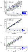 |
Fig. 7. Comparison between the chemical abundances and U values introduced as inputs for the models (x-axis) with the estimations from HCM-IR when all lines plus [S III]λ33 μm are used (y-axis). For all plots we present Seyferts as blue circles and LINERs as green squares. The offsets are given using the median value (dashed line) and RMSE (dot-dashed lines). Bottom plots show the residuals from the offset and their distribution in a histogram (bottom-right plot). |
From Figs. 8a, c, and e, we conclude that no significant change is introduced in the chemical abundances or ionization parameters derived when the grid of models is computed assuming an SED characterized by αOX = −1.2; the offsets are below 0.05 dex and the RMSE is always below the step considered in the grid for the given quantity. On the other hand, the effects of selecting a different stopping criteria are more notorious in the determination of the ionization parameter; high-ionization (U > −2.5) AGN present a higher scatter, with values clustering around log(U) ∼ −1.8. This effect is mainly caused due to changes in the emission lines of highly ionizing species such as Ne4+ or O3+. In the case of O/H, there seems to be a slight overestimation when models with stopping criteria of 98% free electrons are considered. N/O does not show any significant change.
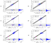 |
Fig. 8. Comparison between the chemical abundances and U values introduced, obtained from the grid characterized by αOX = −0.8 and a 2% fraction of free electrons (x-axis) with models with αOX = −1.2 ((a), (c), and (e)) and models with 98% as stopping criteria ((b), (d), and (f)). For all plots we present Seyferts as blue circles, ULIRGs as green squares, LIRGs as magenta triangles, and LINERs as red stars. The offsets are given using the median value (dashed line) and RMSE (dot-dashed lines). Bottom plots show the residuals from the offset and their distribution in a histogram (bottom-right plot). |
4. Results
We present in this section the chemical abundances and ionization parameters estimated for our sample of AGN using HCM-IR. Due to the lack of alternatives to estimate these parameters from IR observations of AGN, we use optical spectroscopic information of the same sample in order to compare results from both sets of information.
4.1. Infrared estimations
We summarize in Table 3 the statistics of the estimations of the chemical abundances and log(U) values obtained with HCM-IR from the IR emission lines in our sample distinguishing between different types of galaxies. Table A.2 shows these results in detail for each galaxy in our sample.
Statistics of the chemical abundances and log(U) values derived from HCM-IR for our sample of galaxies.
As expected from our preliminary distinction of AGN, we have two main subgroups based on U results consistent with our prior distinction; Seyferts belong to the high-ionization AGN category, as they usually present log(U) > −2.5 (Ho et al. 1993; Villar-Martín et al. 2008; Zhuang et al. 2019), while LINERs fall in the category of low-ionization AGN with log(U) < −2.5 (Ferland & Netzer 1983; Halpern & Steiner 1983; Binette 1985; Kewley et al. 2006). In the case of ULIRGs and LIRGs, the study by Pereira-Santaella et al. (2017) showed that low (log(U) < −2.5) ionization parameters are needed to reproduce observations from photoionization models, and thus we assume they fall in the category of low-ionization AGN.
Although we have relatively low statistics, the three spectral types considered as low-ionization AGN differ in their median ionization; ULIRGs show the highest value (U ∼ −3), followed by LINERs (U ∼ −3.25) and then by LIRGs (U ∼ −3.6). Despite these differences being higher than their dispersions, they are still close to the step for U used in the grid (0.25 dex) of models, and thus they must be revisited in a larger sample of galaxies.
Analyzing chemical abundances, we obtained median subsolar values for all types of galaxies, Seyferts being, on average, metal-poorer than the other three spectral types. However, since the estimation of 12+log(O/H) is only available in the few galaxies with detected hydrogen recombination lines, this result must be revisited in larger samples of galaxies. N/O shows a similar median value for all types of galaxies, clustering around the solar value of log(N/O)⊙ = −0.86 (Asplund et al. 2009).
We also present in Fig. 9 the well-known N/O-O/H diagram obtained from our IR estimations. It should be noted that our statistics for this plot are small because we need galaxies with estimations of both log(N/O) and 12+log(O/H). We find almost a flattened behavior around log(N/O)⊙, although there are some galaxies with higher ratios.
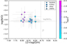 |
Fig. 9. N/O vs. O/H from IR estimations. The values for log(U) are given by the colorbar. |
4.2. Optical estimations
We compiled, from the literature, optical emission-line fluxes for our sample of AGN, and corrected all emission-line ratios for reddening (see Table A.3) relative to the Balmer line Hβ, following Howarth’s extinction curve (Howarth 1983), assuming RV = 3.1 and a theoretical ratio between Hα and Hβ of 3.1, characteristic of the Recombination Case B for the physical conditions of the NLR in AGN. Although we have additional information from IR observations, which are necessary in order to account for some ionic species whose emission lines cannot be retrieved from optical emission lines, such as O3+, and this can in turn lead to underestimations in the oxygen abundance (Dors et al. 2015; Maiolino & Mannucci 2019; Flury & Moran 2020), we cannot apply the direct method since only two galaxies in our sample (namely Mrk 478 and NGC 4151) present measurements of auroral line [O III]λ4363Å, which are key for determining the electronic temperature Te of the ISM. Thus, we estimated chemical abundances from optical emission lines for our sample of AGN using the optical version of HCM for AGN (PM19). The code takes as input the following reddening-corrected optical emission lines: [O II]λ3727Å, [Ne III]λ3868Å, [O III]λ4363Å, [O III]λ5007Å, [N II]λ6584Å, and [S II]λλ6717,6731Å; all of them are relative to the Balmer line Hβ.
To check our optical estimations, we also considered the calibration proposed by Flury & Moran (2020) based on [O III]λ5007Å and [N II]λ6584Å, given by:
 (12)
(12)
where u = log(I([N II]λ6584Å/Hα)) and v = log(I( [O III]λ5007Å/Hβ)). This calibration is valid for the range 7.5 ≤ 12+log(O/H) ≤ 9.0.
We also considered the calibration based on the N line [N II]λ6584Å given by Carvalho et al. (2020):
where N2 = log(I(([N II]λ6584Å/Hβ)) , a = 4.01 ± 0.08, and b = −0.07 ± 0.01. In terms of the oxygen abundance, the calibration is given by3:
 (13)
(13)
which was defined in the range 8.17 ≤ 12+log(O/H) ≤ 9.0.
We compared the resulting abundances in our sample of AGN (see Table A.4) from the calibrations described above with those from HCM in Fig. 10. The calibration proposed by Flury & Moran (2020) tends to underestimate HCM abundances, with a median offset of −0.39 dex. On the other hand, the calibration proposed by Carvalho et al. (2020) better fits our results, with a median offset of 0.14 dex. As shown in bottom plot of Fig. 7b, the discrepancy is higher for ULIRGs, LIRGs, and LINERs than for Seyferts. This could be explained by the fact that Carvalho et al. (2020) obtained their calibration from a sample of Seyferts 2 from the Sloan Digital Sky Survey (SDSS), in other words it was obtained using only high-ionization AGN, covering a different range of the ionization parameter to the values reported for low-ionization AGN (e.g., Kewley et al. 2006). Another possible source of error is that the calibration is based only on a nitrogen line, so it assumes a relation between 12+log(O/H) and log(N/O), although it has been reported that both quantities might not be related in low-ionization AGN (Pérez-Díaz et al. 2021).
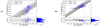 |
Fig. 10. Chemical abundances derived from optical emission lines in our sample of AGN. (a) Comparison between the chemical abundances derived with the calibration from Flury & Moran (2020; y-axis), denoted as FM20, and HCM (x-axis). (b) Comparison between the chemical abundances derived from the calibration from Carvalho et al. (2020; y-axis), denoted as FM20, with HCM (x-axis). For all plots we present Seyferts as blue circles, ULIRGs as green squares, LIRGs as magenta triangles, and LINERs as red stars. The offsets are given using the median value (dashed line) and RMSE (dot-dashed lines). Bottom plots show the residuals from the offset and their distribution in a histogram (bottom-right plot). |
We present in Table 4 the statistics of the chemical abundances derived from the optical version of the code. Again, we find that 12+log(O/H) presents subsolar median values for all types of galaxies. The median N/O values present more variation between different types but, considering the standard deviations, they are still compatible with them, and with the solar value obtained from IR estimations.
We also present in Fig. 11 the N/O–O/H diagram. We can see two different trends based on the two main categories considered throughout this study. For low-luminosity AGN (ULIRGs, LIRGs, and LINERs) there seems to be an anticorrelation between N/O and O/H (although the corresponding Pearson coefficient correlation is low r ∼ −0.75). In the case of high-ionization AGN, both quantities do not seem to be correlated, which was also found by Pérez-Díaz et al. (2021), although with a smaller sample of galaxies. As AGN activity is a rare phenomenon among dwarf galaxies (< 1.8%, Latimer et al. 2021), and these have been challenging targets for previous IR spectroscopic facilities, our N/O versus O/H diagram cannot reproduce the metal-poor regime with sufficient statistics.
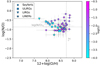 |
Fig. 11. N/O vs. O/H as derived from optical estimations. The log(U) values are given by the colorbar. |
4.3. Optical versus infrared estimations
Comparing the results listed in Tables 3 and 4, we can see that Seyferts present lower median oxygen abundances from IR estimations than from their optical counterpart, the average offset for high-ionization AGN being higher than 0.5 dex. Although lower, we also found an average offset of 0.3 dex between optical and IR estimations for LINERs. While ULIRGs present similar oxygen abundances from both methods, in the case of LIRGs, we obtain lower abundances from optical observations. However, this result must be revisited using larger samples of galaxies, given our low statistic for LIRGs.
From Fig. 12a we can see that 12+log(O/H) values from IR emission lines are systematically lower than the abundances derived using optical lines, which agrees with our previous statement for Seyferts. In the case of N/O, we obtained IR values clustering around the solar abundance, while optical estimations present a wider range of values, as shown in Fig. 12b. Finally, in Fig. 12c we compare the resulting log(U) values, obtaining slightly higher values from IR estimations overall. However, since the step of the grids is 0.25 dex in log(U), and both the median offset and RMSE are close to this value, we can conclude that little difference is found.
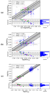 |
Fig. 12. Comparison between the chemical abundances and log(U) values obtained from optical emission lines using HCM (x-axis) and the corresponding estimations from IR lines using HCM-IR (y-axis). For all plots we present Seyferts as blue circles, ULIRGs as green squares, LIRGs as magenta triangles, and LINERs as red stars. The offsets are given using the median value (dashed line) and RMSE (dot-dashed lines). Bottom plots show the residuals from the offset and their distribution in a histogram (bottom-right plot). |
4.4. Dependency of the discrepancies
As pointed out in the previous section, there is a significant difference between optical and infrared estimations of chemical abundances. Hereinafter, we define the discrepancy for a given quantity X as ΔX = Xopt − Xir.
We present in Fig. 13 the discrepancy as a function of the two chemical abundance ratios (12+log(O/H) and log(N/O)) for IR (left column) and optical estimations (right column). Figures 13a and c shows that little correlation is found between the discrepancies and their corresponding abundances from IR emission lines. This is not the case in the optical range as previously discussed: Δ log(O/H) increases with the oxygen abundance (see Fig. 13b). A similar result is also found for Δ log(N/O) (see Fig. 13d).
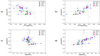 |
Fig. 13. Discrepancies between the chemical abundance ratios (ΔX = Xopt − XIR) as a function of their ratios: (a) 12+log(O/H) and (c) log(N/O) both derived from IR emission lines with HCM-IR, and (b) 12+log(O/H) and (d) log(N/O) derived from optical emission lines with HCM. For all plots we present Seyferts as blue circles, ULIRGs as green squares, LIRGs as magenta triangles, and LINERs as red stars. |
We replicate the same study of the discrepancies as a function of the ionization parameter U. Figure 14 shows that U (either derived from optical emission lines or IR emission lines) does not drive the discrepancies found for both O/H and N/O.
In Sect. 3.1 we explained the importance of electronic density for IR emission lines, since for wavelengths in far-IR (above 80 μm) the corresponding critical densities nc of the lines are closer to the expected ne ∼ 500 cm−3 for the NLR of AGN (Alloin et al. 2006; Vaona et al. 2012; Netzer 2015). This is not the case for optical emission lines whose critical densities are in the range [103.5, 106] cm−3.
We estimated electronic densities from both optical and IR emission lines, using PYNEB (Luridiana et al. 2015) and assuming an electronic temperature Te ∼ 2 × 10⁴ K, which is the average electronic temperature of the different ionic species in the models. We used the sulfur doublet [S II]λλ6717,6731Å for our optical determination and the sulfur lines [S III]λ 18 μm and [S III]λ 33μm to estimate ne from IR lines.
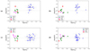 |
Fig. 14. Discrepancies between the chemical abundance ratios (ΔX = Xopt − XIR) as a function of the ionization parameter: (a) and (c) estimated from IR lines, (b) and (d) estimated from optical lines. |
As shown in Fig. 15, neither Δlog(O/H) nor Δlog(N/O) correlate with electronic density. This result was also found by Spinoglio et al. (2022), although they only analyzed nitrogen-to-oxygen abundances in a sample of AGN from SOFIA due to the spectral coverage. Our results extend this behavior to the oxygen abundances.
 |
Fig. 15. Discrepancies between the chemical abundance ratios (ΔX = Xopt − XIR) as a function of the electronic density: (a) and (c) present electronic densities derived from [S III] lines, (b) and (d) present densities derived from [S II] lines. |
5. Discussion
5.1. Abundances from IR lines
IR emission lines are key for analyzing chemical abundances in both dusty-embedded regions and from the cold component (∼1000 K) of the ionized gas, which is barely accessible for optical observations. However, in general, we warn the reader about the reduced statistics in our sample of galaxies with a reliable derivation of O/H (below 50% of our sample), due to the lack of measurements of hydrogen lines. On the other hand, slightly better statistics are found in N/O (∼60%), but again the measurement of [N III]λ57 μm is critical for that estimation. Overall, the estimation of U is almost assured when running the code (∼90%). Nevertheless, these results must be corroborated in larger samples of AGN.
Our estimations of chemical abundances in the NLR of AGN show that the infrared emission is tracing a region characterized by subsolar oxygen abundances (12+log(O/H) < 8.69). Since the measurement of at least one hydrogen line is necessary to provide an estimation of O/H, these subsolar values might be explained by an intrinsic bias: galaxies with measurements of hydrogen emission lines may be characterized by low metallicities. Moreover, as estimations of oxygen abundances require the measurement of faint emission lines as hydrogen recombination lines, these measurements are always obtained with higher uncertainties (see Table 2). Unfortunately, the lack of alternative methodologies to directly estimate IR oxygen abundances does not allow us to test this hypothesis.
The N/O ratio seems to be constant for this sample, clustering around the solar value log(N/O)⊙ = −1.06. In fact, N/O abundances are well constrained in the range [−1.1, −0.4], which is the same range reported by Spinoglio et al. (2022) for their sample of AGN.
The lack of an apparent correlation between N/O and O/H (see Fig. 10), contrary to other assumed relations in the same metallicity regime, evidences that using nitrogen emission lines to estimate oxygen abundances must rely on an independent measurement of N/O, which can also be done by HCM-IR. The assumption of different relations between N/O and O/H could thus produce nonnegligible deviations in the estimated O/H value as derived using N lines. For instance, contrary to our results, Chartab et al. (2022) reported oxygen abundances above the solar value by assuming a N/O-O/H relation and a fixed ionization parameter U. This discrepancy, also observed by FO21 for SFGs (showing little offset between IR and optical estimations), might be explained by the different assumption of an N/O–O/H relation for IR estimations.
5.2. Discrepancies between IR and optical estimations
While the estimations of the ionization parameter U derived from IR emission-lines are consistent with those derived from optical lines for low-ionization AGN, although with slightly more scatter for high-ionization objects (see Fig. 12c), we report an offset between the estimated chemical abundances from IR and from optical lines. From Fig. 12a we find that the Δlog(O/H) discrepancy is higher for the more metallic AGN (see also Fig. 13d); using IR emission lines values above solar oxygen abundances cannot be reached, although there are galaxies in our sample whose optical estimations point toward oversolar abundances. This result is found for Seyferts, but also for ULIRGs and LINERs, which contrasts with the results from Chartab et al. (2022), pointing to chemical abundances estimated from IR lines in a sample of ULIRGs higher than those obtained from optical lines.
Regarding nitrogen-to-oxygen abundance ratios, these follow the same trend: their estimations from optical emission lines are higher than those from IR observations (see Fig. 12b). This result was also found for both SFGs (Peng et al. 2021) and AGN (Spinoglio et al. 2022), although they only use the N3O3 estimator to derive N/O (see Eq. (1)), while we use both N3O3 and N3S34 (see Eq. (2)). Furthermore, we obtained N/O abundances clustering around N/O⊙, in agreement with the results by Spinoglio et al. (2022).
These discrepancies between N/O and O/H from optical and IR observations also translate into the N/O–O/H diagram (see Figs. 9 and 11). While there is a trend of decreasing N/O for increasing O/H for low-ionization AGN, this is not found when IR estimations are considered. In the case of Seyferts, the range of values for O/H and N/O is more limited from IR estimations than from optical estimations. Thus, we warn the reader about using any N/O–O/H relation to estimate oxygen abundances from IR nitrogen lines, especially if this relation was obtained from optical observations.
As evidenced by Fig. 15, these discrepancies cannot be explained by a difference in the electronic density in the observed region. On the contrary, as proposed by Peng et al. (2021), such a difference could ultimately indicate a large contribution from the diffuse ionized gas (DIG) to the estimated chemical abundances.
Another proposed scenario, based on the results for N/O (Peng et al. 2021; Spinoglio et al. 2022), is related to the ionization structure of the gas : IR lines trace high-ionization gas (O++, N++, S++, S3+), while optical lines trace low-ionization gas (O+, N+, S+). If the ionization structure plays a role in these discrepancies found for both O/H and N/O, a trend must appear when these variations are analyzed as a function of U. As shown by Fig. 14, the ionization parameter, either obtained from optical lines ((a) and (c)) or from IR lines ((b) and (d)), shows no correlation with the discrepancies in both O/H and N/O. Thus, the different ionization structure cannot explain the differences obtained between IR and optical estimations of chemical abundances.
In any case, since we are analyzing the NLR in AGN, which is not obscured by the dusty torus, it seems unlikely that dusty-embedded regions of the AGN contribute to these discrepancies, although dust content within the NLR might be underestimated. However, an alternative possible explanation for these discrepancies could arise from the contribution of colder parts in the NLR, whose emission is detected in the IR range. According to our results, these zones could then be characterized by solar values of N/O and subsolar oxygen abundances, which could be consistent with our result that the differences arise above all in the most metallic galaxies.
In the case of AGN, another possible explanation could rely on the spectral resolution of the IR observations. Due to the emission of the broad line region (BLR), hydrogen recombination lines might present an additional contribution to their fluxes from these broad components, which cannot be spectrally resolved with the current IR data. However, this is not the case for the N/O abundance ratios, whose values are estimated independently of the hydrogen recombination lines, and thus an additional contribution to the chemical discrepancies may be present.
5.3. The importance of N/O
Overall, we emphasize that determining nitrogen-to-oxygen abundance is fundamental in order to understand the chemical composition and evolution of the ISM. First of all, as shown in Fig. 2, this ratio does not show a high discrepancy between SFG and AGN models, implying that no bias is introduced if a galaxy is wrongly classified. Although the difference arises for N3S34, N3O3 has proved to be a robust N/O estimator for both AGN and SFGs.
Secondly, the estimations of N/O involved close IR emission lines, such as [O III]λ52 μm, [N III]λ57 μm, or [O III]λ88 μm, which are more likely to be accessible in the same observational set. Thanks to the ongoing mission SOFIA, some of these emission lines are detected for galaxies in the local Universe, and current and future ground-based submillimeter telescopes (e.g., ALMA) will retrieve these lines for the rest-frame IR spectrum of high-redshift galaxies, allowing a redshift-dependent study of N/O.
Thirdly, this chemical abundance ratio is necessary in order to provide an unbiased estimation of oxygen abundances from nitrogen emission lines. As pointed out by several authors (e.g., Pérez-Montero & Contini 2009; Pérez-Díaz et al. 2021; Fernández-Ontiveros et al. 2021; Spinoglio et al. 2022), assuming an arbitrary law for N/O-O/H, which is not always followed, can lead to uncertainties in the oxygen content of the gas-phase, and this can be avoided when data allows an independent previous determination of N/O.
Finally, since N/O involves the abundance of a metal with primary origin (O) and the abundance of another metal with a possible secondary origin (N), its determination also provides key information on the chemical evolution of the metals in the ISM.
6. Conclusions
We have presented HII-CHI-MISTRY-IR for AGN, an updated version of the code proposed for SFGs. Thanks to this new method, chemical abundances in the NLR of AGN can be estimated from IR nebular emission lines, which are less affected by extinction and show little dependence on physical conditions of the ISM as the electronic density or temperature. This new tool allows, whenever possible, an independent estimation of N/O, O/H, and U.
The analysis of a sample of AGN with available IR emission-line fluxes compiled from the literature shows that their oxygen abundances tend to be solar and subsolar (12+log(O/H) ≤ 8.69), while nitrogen-to-oxygen abundance ratios cluster around solar values (log(N/O) ∼ −1). Since both O/H and N/O are calculated independently, these new estimations show that a relation between N/O-O/H is not found for our sample of AGN.
We also estimated chemical abundances from optical observations of the same sample of AGN. In general, higher oxygen abundances are obtained from these estimations than from IR observations. An analogous result is also found for nitrogen-to-oxygen ratios. We explored if these discrepancies between optical and IR observations arise from the contribution of diffuse ionized gas, but we concluded that they are not related to electronic density. We also find that these discrepancies do not correlate with the ionizing field. As these differences are found for most metallic AGN, IR emission could trace zones of the AGN characterized by subsolar oxygen abundances and solar nitrogen-to-oxygen ratios.
In the coming years, thanks to JWST and METIS for the local Universe, and ALMA, APEX, and CSO for high-redshift galaxies, the amount of galaxies (including AGN), whose IR spectral information will be retrieved with high precision, will notably increase, leading to a higher volume of AGN with IR hydrogen recombination lines measured and with many other fine-structure IR lines. With this upcoming data, further constraints can be established for the IR N/O-O/H relation, and for the systematic offset between IR and optical estimations.
As analogous to the optical diagnostic diagrams, also called Baldwin, Phillips & Terlevich (BPT) diagrams.
All versions of the HII-CHI-MISTRY code are publicly available at: http://www.iaa.csic.es/~epm/HII-CHI-mistry.html.
We assume here the solar abundances from Asplund et al. (2009).
Acknowledgments
We acknowledge support from the Spanish MINECO grants AYA2016-76682C3-1-P, AYA2016-79724-C4 and PID2019-106027GB-C41. We also acknowledge financial support from the State Agency for Research of the Spanish MCIU through the “Center of Excellence Severo Ochoa” award to the Instituto de Astrofísica de Andalucía (SEV-2017-0709). JAFO acknowledges the financial support from the Spanish Ministry of Science and Innovation and the European Union – NextGenerationEU through the Recovery and Resilience Facility project ICTS-MRR-2021-03-CEFCA. We acknowledge the fruitful discussions with our research team. We thank the anonymous referee for the constructive report that improved this manuscript. E.P.M. acknowledges the assistance from his guide dog Rocko without whose daily help this work would have been much more difficult.
References
- Aller, L. H. 1984, Physics of Thermal Gaseous Nebulae, Astrophysics and Space Science Library, (Dordrecht: Reidel) [Google Scholar]
- Alloin, D., Johnson, R., & Lira, P. 2006, Physics of Active Galactic Nuclei at all Scales (Springer), 693 [CrossRef] [Google Scholar]
- Alonso-Herrero, A., Rieke, G. H., Rieke, M. J., & Scoville, N. Z. 2000, ApJ, 532, 845 [NASA ADS] [CrossRef] [Google Scholar]
- Amorín, R. O., Pérez-Montero, E., & Vílchez, J. M. 2010, ApJ, 715, L128 [CrossRef] [Google Scholar]
- Andrews, B. H., & Martini, P. 2013, ApJ, 765, 140 [NASA ADS] [CrossRef] [Google Scholar]
- Armus, L., Charmandaris, V., Bernard-Salas, J., et al. 2007, ApJ, 656, 148 [NASA ADS] [CrossRef] [Google Scholar]
- Asplund, M., Grevesse, N., Sauval, A. J., & Scott, P. 2009, ARA&A, 47, 481 [NASA ADS] [CrossRef] [Google Scholar]
- Baldwin, J. A., Phillips, M. M., & Terlevich, R. 1981, PASP, 93, 5 [Google Scholar]
- Bellamy, M. J., & Tadhunter, C. N. 2004, MNRAS, 353, 105 [NASA ADS] [CrossRef] [Google Scholar]
- Bellamy, M. J., Tadhunter, C. N., Morganti, R., et al. 2003, MNRAS, 344, L80 [CrossRef] [Google Scholar]
- Bendo, G. J., & Joseph, R. D. 2004, AJ, 127, 3338 [NASA ADS] [CrossRef] [Google Scholar]
- Bennert, N., Jungwiert, B., Komossa, S., Haas, M., & Chini, R. 2006a, A&A, 459, 55 [NASA ADS] [CrossRef] [EDP Sciences] [Google Scholar]
- Bennert, N., Jungwiert, B., Komossa, S., Haas, M., & Chini, R. 2006b, A&A, 456, 953 [NASA ADS] [CrossRef] [EDP Sciences] [Google Scholar]
- Berg, D. A., Skillman, E. D., Henry, R. B. C., Erb, D. K., & Carigi, L. 2016, ApJ, 827, 126 [NASA ADS] [CrossRef] [Google Scholar]
- Bernard-Salas, J., Spoon, H. W. W., Charmandaris, V., et al. 2009, ApJS, 184, 230 [Google Scholar]
- Binette, L. 1985, A&A, 143, 334 [NASA ADS] [Google Scholar]
- Boksenberg, A., Shortridge, K., Allen, D. A., et al. 1975, MNRAS, 173, 381 [NASA ADS] [CrossRef] [Google Scholar]
- Brandl, B., Bettonvil, F., van Boekel, R., et al. 2021, The Messenger, 182, 22 [NASA ADS] [Google Scholar]
- Brauher, J. R., Dale, D. A., & Helou, G. 2008, ApJS, 178, 280 [NASA ADS] [CrossRef] [Google Scholar]
- Buchanan, C. L., McGregor, P. J., Bicknell, G. V., & Dopita, M. A. 2006, AJ, 132, 27 [NASA ADS] [CrossRef] [Google Scholar]
- Buttiglione, S., Capetti, A., Celotti, A., et al. 2009, A&A, 495, 1033 [NASA ADS] [CrossRef] [EDP Sciences] [Google Scholar]
- Carvalho, S. P., Dors, O. L., Cardaci, M. V., et al. 2020, MNRAS, 492, 5675 [NASA ADS] [CrossRef] [Google Scholar]
- Chartab, N., Cooray, A., Ma, J., et al. 2022, Nature, 6, 844 [NASA ADS] [Google Scholar]
- Chiappini, C., Matteucci, F., & Ballero, S. K. 2005, A&A, 437, 429 [NASA ADS] [CrossRef] [EDP Sciences] [Google Scholar]
- Contini, M. 2012, MNRAS, 426, 719 [NASA ADS] [CrossRef] [Google Scholar]
- Contini, M., & Viegas, S. M. 2001, ApJS, 137, 75 [NASA ADS] [CrossRef] [Google Scholar]
- Costero, R., & Osterbrock, D. E. 1977, ApJ, 211, 675 [NASA ADS] [CrossRef] [Google Scholar]
- Croxall, K. V., Smith, J. D., Brandl, B. R., et al. 2013, ApJ, 777, 96 [Google Scholar]
- Curti, M., Cresci, G., Mannucci, F., et al. 2017, MNRAS, 465, 1384 [Google Scholar]
- Cyburt, R. H., Fields, B. D., Olive, K. A., & Yeh, T.-H. 2016, Rev. Mod. Phys., 88, 015004 [NASA ADS] [CrossRef] [Google Scholar]
- Dannerbauer, H., Rigopoulou, D., Lutz, D., et al. 2005, A&A, 441, 999 [NASA ADS] [CrossRef] [EDP Sciences] [Google Scholar]
- Dors, O. L., Hägele, G. F., Cardaci, M. V., et al. 2013, MNRAS, 432, 2512 [NASA ADS] [CrossRef] [Google Scholar]
- Dors, O. L., Cardaci, M. V., Hägele, G. F., & Krabbe, A. C. 2014, MNRAS, 443, 1291 [NASA ADS] [CrossRef] [Google Scholar]
- Dors, O. L., Cardaci, M. V., Hägele, G. F., et al. 2015, MNRAS, 453, 4102 [Google Scholar]
- Dors, O. L., Monteiro, A. F., Cardaci, M. V., Hägele, G. F., & Krabbe, A. C. 2019, MNRAS, 486, 5853 [NASA ADS] [CrossRef] [Google Scholar]
- Duc, P. A., Mirabel, I. F., & Maza, J. 1997, A&AS, 124, 533 [NASA ADS] [CrossRef] [EDP Sciences] [Google Scholar]
- Durret, F., & Bergeron, J. 1988, A&AS, 75, 273 [NASA ADS] [Google Scholar]
- Erb, D. K., Pettini, M., Shapley, A. E., et al. 2010, ApJ, 719, 1168 [Google Scholar]
- Erkens, U., Appenzeller, I., & Wagner, S. 1997, A&A, 323, 707 [NASA ADS] [Google Scholar]
- Ferland, G. J., & Netzer, H. 1983, ApJ, 264, 105 [NASA ADS] [CrossRef] [Google Scholar]
- Ferland, G. J., Chatzikos, M., Guzmán, F., et al. 2017, Rev. Mex. Astron. Astrofis., 53, 385 [NASA ADS] [Google Scholar]
- Fernández-Ontiveros, J. A., Spinoglio, L., Pereira-Santaella, M., et al. 2016, ApJS, 226, 19 [CrossRef] [Google Scholar]
- Fernández-Ontiveros, J. A., Pérez-Montero, E., Vílchez, J. M., Amorín, R., & Spinoglio, L. 2021, A&A, 652, A23 [NASA ADS] [CrossRef] [EDP Sciences] [Google Scholar]
- Fischer, C., Beckmann, S., Bryant, A., et al. 2018, J. Astron. Instrum., 7, 1840003 [Google Scholar]
- Flury, S. R., & Moran, E. C. 2020, MNRAS, 496, 2191 [NASA ADS] [CrossRef] [Google Scholar]
- García-Marín, M., Colina, L., Arribas, S., Alonso-Herrero, A., & Mediavilla, E. 2006, ApJ, 650, 850 [CrossRef] [Google Scholar]
- Garnett, D. R., & Shields, G. A. 1987, ApJ, 317, 82 [NASA ADS] [CrossRef] [Google Scholar]
- Genzel, R., Lutz, D., Sturm, E., et al. 1998, ApJ, 498, 579 [Google Scholar]
- Goldader, J. D., Joseph, R. D., Doyon, R., & Sanders, D. B. 1995, ApJ, 444, 97 [NASA ADS] [CrossRef] [Google Scholar]
- González Delgado, R. M., & Leitherer, C. 1999, ApJS, 125, 479 [CrossRef] [Google Scholar]
- Goodrich, R. W., & Osterbrock, D. E. 1983, ApJ, 269, 416 [NASA ADS] [CrossRef] [Google Scholar]
- Gu, Q., Melnick, J., Cid Fernandes, R., et al. 2006, MNRAS, 366, 480 [NASA ADS] [CrossRef] [Google Scholar]
- Guseva, N. G., Izotov, Y. I., Schaerer, D., et al. 2020, MNRAS, 497, 4293 [CrossRef] [Google Scholar]
- Halpern, J. P., & Steiner, J. E. 1983, ApJ, 269, L37 [CrossRef] [Google Scholar]
- Hayden-Pawson, C., Curti, M., Maiolino, R., et al. 2022, MNRAS, 512, 2867 [NASA ADS] [CrossRef] [Google Scholar]
- Herrera-Camus, R., Sturm, E., Graciá-Carpio, J., et al. 2018, ApJ, 861, 94 [Google Scholar]
- Ho, L. C., Shields, J. C., & Filippenko, A. V. 1993, ApJ, 410, 567 [NASA ADS] [CrossRef] [Google Scholar]
- Ho, L. C., Filippenko, A. V., & Sargent, W. L. W. 1997, ApJS, 112, 315 [NASA ADS] [CrossRef] [Google Scholar]
- Houck, J. R., Roellig, T. L., van Cleve, J., et al. 2004, ApJS, 154, 18 [NASA ADS] [CrossRef] [Google Scholar]
- Howarth, I. D. 1983, MNRAS, 203, 301 [NASA ADS] [CrossRef] [Google Scholar]
- Imanishi, M., & Wada, K. 2004, ApJ, 617, 214 [NASA ADS] [CrossRef] [Google Scholar]
- Imanishi, M., Nakagawa, T., Shirahata, M., Ohyama, Y., & Onaka, T. 2010, ApJ, 721, 1233 [CrossRef] [Google Scholar]
- Inami, H., Armus, L., Charmandaris, V., et al. 2013, ApJ, 777, 156 [Google Scholar]
- Inami, H., Armus, L., Matsuhara, H., et al. 2018, A&A, 617, A130 [NASA ADS] [CrossRef] [EDP Sciences] [Google Scholar]
- Izotov, Y. I., Thuan, T. X., & Privon, G. 2012, MNRAS, 427, 1229 [NASA ADS] [CrossRef] [Google Scholar]
- Kauffmann, G., Heckman, T. M., Tremonti, C., et al. 2003, MNRAS, 346, 1055 [Google Scholar]
- Kessler, M. F., Steinz, J. A., Anderegg, M. E., et al. 1996, A&A, 315, L27 [NASA ADS] [Google Scholar]
- Kewley, L. J., Groves, B., Kauffmann, G., & Heckman, T. 2006, MNRAS, 372, 961 [Google Scholar]
- Kewley, L. J., Nicholls, D. C., & Sutherland, R. S. 2019, ARA&A, 57, 511 [Google Scholar]
- Kim, D. C., Sanders, D. B., Veilleux, S., Mazzarella, J. M., & Soifer, B. T. 1995, ApJS, 98, 129 [NASA ADS] [CrossRef] [Google Scholar]
- Kim, D. C., Veilleux, S., & Sanders, D. B. 1998, ApJ, 508, 627 [NASA ADS] [CrossRef] [Google Scholar]
- Koski, A. T. 1978, ApJ, 223, 56 [NASA ADS] [CrossRef] [Google Scholar]
- Koss, M., Trakhtenbrot, B., Ricci, C., et al. 2017, ApJ, 850, 74 [Google Scholar]
- Kraemer, S. B., Wu, C.-C., Crenshaw, D. M., & Harrington, J. P. 1994, ApJ, 435, 171 [NASA ADS] [CrossRef] [Google Scholar]
- LaMassa, S. M., Heckman, T. M., Ptak, A., et al. 2010, ApJ, 720, 786 [NASA ADS] [CrossRef] [Google Scholar]
- Lamperti, I., Koss, M., Trakhtenbrot, B., et al. 2017, MNRAS, 467, 540 [Google Scholar]
- Lancon, A., Rocca-Volmerange, B., & Thuan, T. X. 1996, A&AS, 115, 253 [NASA ADS] [Google Scholar]
- Latimer, L. J., Reines, A. E., Bogdan, A., & Kraft, R. 2021, ApJ, 922, L40 [NASA ADS] [CrossRef] [Google Scholar]
- Lebouteiller, V., Barry, D. J., Goes, C., et al. 2015, ApJS, 218, 21 [Google Scholar]
- Lequeux, J., Peimbert, M., Rayo, J. F., Serrano, A., & Torres-Peimbert, S. 1979, A&A, 80, 155 [Google Scholar]
- Lumsden, S. L., Heisler, C. A., Bailey, J. A., Hough, J. H., & Young, S. 2001, MNRAS, 327, 459 [NASA ADS] [CrossRef] [Google Scholar]
- Luridiana, V., Morisset, C., & Shaw, R. A. 2015, A&A, 573, A42 [NASA ADS] [CrossRef] [EDP Sciences] [Google Scholar]
- Lutz, D., Maiolino, R., Moorwood, A. F. M., et al. 2002, A&A, 396, 439 [NASA ADS] [CrossRef] [EDP Sciences] [Google Scholar]
- Maiolino, R., & Mannucci, F. 2019, A&ARv, 27, 3 [Google Scholar]
- Malkan, M. A. 1986, ApJ, 310, 679 [NASA ADS] [CrossRef] [Google Scholar]
- Malkan, M. A., Jensen, L. D., Rodriguez, D. R., Spinoglio, L., & Rush, B. 2017, ApJ, 846, 102 [NASA ADS] [CrossRef] [Google Scholar]
- Martins, L. P., Rodríguez-Ardila, A., de Souza, R., & Gruenwald, R. 2010, MNRAS, 406, 2168 [NASA ADS] [CrossRef] [Google Scholar]
- Masters, D., Faisst, A., & Capak, P. 2016, ApJ, 828, 18 [NASA ADS] [CrossRef] [Google Scholar]
- McClure, R. D., & van den Bergh, S. 1968, AJ, 73, 1008 [NASA ADS] [CrossRef] [Google Scholar]
- Meléndez, M., Kraemer, S. B., Armentrout, B. K., et al. 2008, ApJ, 682, 94 [Google Scholar]
- Moorwood, A. F. M., van der Werf, P. P., Kotilainen, J. K., Marconi, A., & Oliva, E. 1996, A&A, 308, L1 [NASA ADS] [Google Scholar]
- Morris, S. L., & Ward, M. J. 1988, MNRAS, 230, 639 [NASA ADS] [CrossRef] [Google Scholar]
- Moustakas, J., & Kennicutt, Jr., R. C. 2006, ApJS, 164, 81 [CrossRef] [Google Scholar]
- Müller-Sánchez, F., Prieto, M. A., Hicks, E. K. S., et al. 2011, ApJ, 739, 69 [Google Scholar]
- Murphy, T. W. J., Soifer, B. T., Matthews, K., Armus, L., & Kiger, J. R. 2001, AJ, 121, 97 [NASA ADS] [CrossRef] [Google Scholar]
- Nagao, T., Maiolino, R., Marconi, A., & Matsuhara, H. 2011, A&A, 526, A149 [NASA ADS] [CrossRef] [EDP Sciences] [Google Scholar]
- Netzer, H. 2015, ARA&A, 53, 365 [Google Scholar]
- Nomoto, K., Kobayashi, C., & Tominaga, N. 2013, ARA&A, 51, 457 [CrossRef] [Google Scholar]
- Oliva, E., Salvati, M., Moorwood, A. F. M., & Marconi, A. 1994, A&A, 288, 457 [NASA ADS] [Google Scholar]
- Osterbrock, D. E., & Ferland, G. J. 2006, Astrophysics of Ggaseous Nebulae and Active Galactic Nuclei (Sausalito, CA: University Science Books) [Google Scholar]
- Osterbrock, D. E., & Koski, A. T. 1976, MNRAS, 176, 61P [NASA ADS] [CrossRef] [Google Scholar]
- Osterbrock, D. E., & Martel, A. 1993, ApJ, 414, 552 [Google Scholar]
- Osterbrock, D. E., & Miller, J. S. 1975, ApJ, 197, 535 [NASA ADS] [CrossRef] [Google Scholar]
- Pastoriza, M. G. 1979, ApJ, 234, 837 [NASA ADS] [CrossRef] [Google Scholar]
- Peng, B., Lamarche, C., Stacey, G. J., et al. 2021, ApJ, 908, 166 [NASA ADS] [CrossRef] [Google Scholar]
- Pereira-Santaella, M., Rigopoulou, D., Farrah, D., Lebouteiller, V., & Li, J. 2017, MNRAS, 470, 1218 [NASA ADS] [CrossRef] [Google Scholar]
- Pérez-Díaz, B., Masegosa, J., Márquez, I., & Pérez-Montero, E. 2021, MNRAS, 505, 4289 [CrossRef] [Google Scholar]
- Pérez-Montero, E. 2014, MNRAS, 441, 2663 [CrossRef] [Google Scholar]
- Pérez-Montero, E., & Amorín, R. 2017, MNRAS, 467, 1287 [Google Scholar]
- Pérez-Montero, E., & Contini, T. 2009, MNRAS, 398, 949 [CrossRef] [Google Scholar]
- Pérez-Montero, E., Dors, O. L., Vílchez, J. M., et al. 2019, MNRAS, 489, 2652 [CrossRef] [Google Scholar]
- Pérez-Montero, E., Amorín, R., Sánchez Almeida, J., et al. 2021, MNRAS, 504, 1237 [CrossRef] [Google Scholar]
- Pérez-Torres, M., Mattila, S., Alonso-Herrero, A., Aalto, S., & Efstathiou, A. 2021, A&ARv, 29, 2 [CrossRef] [Google Scholar]
- Phillips, M. M. 1978, ApJS, 38, 187 [NASA ADS] [CrossRef] [Google Scholar]
- Phillips, M. M., Charles, P. A., & Baldwin, J. A. 1983, ApJ, 266, 485 [Google Scholar]
- Pilbratt, G. L., Riedinger, J. R., Passvogel, T., et al. 2010, A&A, 518, L1 [NASA ADS] [CrossRef] [EDP Sciences] [Google Scholar]
- Pilyugin, L. S., & Grebel, E. K. 2016, MNRAS, 457, 3678 [NASA ADS] [CrossRef] [Google Scholar]
- Pilyugin, L. S., Vílchez, J. M., & Contini, T. 2004, A&A, 425, 849 [NASA ADS] [CrossRef] [EDP Sciences] [Google Scholar]
- Piqueras López, J., Colina, L., Arribas, S., Alonso-Herrero, A., & Bedregal, A. G. 2012, A&A, 546, A64 [NASA ADS] [CrossRef] [EDP Sciences] [Google Scholar]
- Poglitsch, A., Waelkens, C., Geis, N., et al. 2010, A&A, 518, L2 [NASA ADS] [CrossRef] [EDP Sciences] [Google Scholar]
- Reunanen, J., Kotilainen, J. K., & Prieto, M. A. 2002, MNRAS, 331, 154 [NASA ADS] [CrossRef] [Google Scholar]
- Reunanen, J., Kotilainen, J. K., & Prieto, M. A. 2003, MNRAS, 343, 192 [NASA ADS] [CrossRef] [Google Scholar]
- Rieke, G. H., Wright, G. S., Böker, T., et al. 2015, PASP, 127, 584 [NASA ADS] [CrossRef] [Google Scholar]
- Riffel, R., Rodríguez-Ardila, A., & Pastoriza, M. G. 2006, A&A, 457, 61 [NASA ADS] [CrossRef] [EDP Sciences] [Google Scholar]
- Rigby, J. R., Diamond-Stanic, A. M., & Aniano, G. 2009, ApJ, 700, 1878 [Google Scholar]
- Rupke, D. S. N., Veilleux, S., & Baker, A. J. 2008, ApJ, 674, 172 [NASA ADS] [CrossRef] [Google Scholar]
- Severgnini, P., Risaliti, G., Marconi, A., Maiolino, R., & Salvati, M. 2001, A&A, 368, 44 [NASA ADS] [CrossRef] [EDP Sciences] [Google Scholar]
- Shang, Z., Wills, B. J., Wills, D., & Brotherton, M. S. 2007, AJ, 134, 294 [NASA ADS] [CrossRef] [Google Scholar]
- Shuder, J. M. 1980, ApJ, 240, 32 [NASA ADS] [CrossRef] [Google Scholar]
- Simpson, C., & Meadows, V. 1998, ApJ, 505, L99 [NASA ADS] [CrossRef] [Google Scholar]
- Smajić, S., Fischer, S., Zuther, J., & Eckart, A. 2012, A&A, 544, A105 [NASA ADS] [CrossRef] [EDP Sciences] [Google Scholar]
- Spinoglio, L., Fernandez-Ontiveros, J. A., Malkan, M. A., et al. 2022, ApJ, 926, 55 [NASA ADS] [CrossRef] [Google Scholar]
- Storchi-Bergmann, T., Bica, E., Kinney, A. L., & Bonatto, C. 1997, MNRAS, 290, 231 [NASA ADS] [CrossRef] [Google Scholar]
- Storchi-Bergmann, T., Schmitt, H. R., Calzetti, D., & Kinney, A. L. 1998, AJ, 115, 909 [NASA ADS] [CrossRef] [Google Scholar]
- Sutherland, R. S., & Dopita, M. A. 2017, ApJS, 229, 34 [Google Scholar]
- Temi, P., Marcum, P. M., Young, E., et al. 2014, ApJS, 212, 24 [NASA ADS] [CrossRef] [Google Scholar]
- Thomas, A. D., Kewley, L. J., Dopita, M. A., et al. 2019, ApJ, 874, 100 [NASA ADS] [CrossRef] [Google Scholar]
- Thornley, M. D., Förster Schreiber, N. M., Lutz, D., et al. 2000, ApJ, 539, 641 [NASA ADS] [CrossRef] [Google Scholar]
- Thuan, T. X., Izotov, Y. I., & Lipovetsky, V. A. 1995, ApJ, 445, 108 [NASA ADS] [CrossRef] [Google Scholar]
- Vaceli, M. S., Viegas, S. M., Gruenwald, R., & de Souza, R. E. 1997, AJ, 114, 1345 [NASA ADS] [CrossRef] [Google Scholar]
- Vaona, L., Ciroi, S., Di Mille, F., et al. 2012, MNRAS, 427, 1266 [NASA ADS] [CrossRef] [Google Scholar]
- Veilleux, S., Goodrich, R. W., & Hill, G. J. 1997, ApJ, 477, 631 [NASA ADS] [CrossRef] [Google Scholar]
- Veilleux, S., Kim, D. C., & Sanders, D. B. 1999, ApJ, 522, 113 [NASA ADS] [CrossRef] [Google Scholar]
- Veilleux, S., Rupke, D. S. N., Kim, D. C., et al. 2009, ApJS, 182, 628 [NASA ADS] [CrossRef] [Google Scholar]
- Vila-Costas, M. B., & Edmunds, M. G. 1993, MNRAS, 265, 199 [NASA ADS] [CrossRef] [Google Scholar]
- Villar-Martín, M., Humphrey, A., Martínez-Sansigre, A., et al. 2008, MNRAS, 390, 218 [CrossRef] [Google Scholar]
- Vincenzo, F., & Kobayashi, C. 2018, A&A, 610, L16 [NASA ADS] [CrossRef] [EDP Sciences] [Google Scholar]
- Werner, M. W., Roellig, T. L., Low, F. J., et al. 2004, ApJS, 154, 1 [NASA ADS] [CrossRef] [Google Scholar]
- Westin, B. A. M. 1985, A&A, 151, 137 [NASA ADS] [Google Scholar]
- Wilson, A. S., & Penston, M. V. 1979, ApJ, 232, 389 [NASA ADS] [CrossRef] [Google Scholar]
- Winkler, H. 1992, MNRAS, 257, 677 [NASA ADS] [Google Scholar]
- Wootten, A., & Thompson, A. R. 2009, IEEE Proc., 97, 1463 [NASA ADS] [CrossRef] [Google Scholar]
- Wright, G. S., Wright, D., Goodson, G. B., et al. 2015, PASP, 127, 595 [NASA ADS] [CrossRef] [Google Scholar]
- Wu, H., Zou, Z. L., Xia, X. Y., & Deng, Z. G. 1998, A&AS, 127, 521 [NASA ADS] [CrossRef] [EDP Sciences] [Google Scholar]
- Yano, K., Baba, S., Nakagawa, T., et al. 2021, ApJ, 922, 272 [NASA ADS] [CrossRef] [Google Scholar]
- Yeh, S. C. C., & Matzner, C. D. 2012, ApJ, 757, 108 [NASA ADS] [CrossRef] [Google Scholar]
- Zhuang, M.-Y., Ho, L. C., & Shangguan, J. 2019, ApJ, 873, 103 [NASA ADS] [CrossRef] [Google Scholar]
Appendix A: Data
We present in this appendix the full dataset of mid- to far-IR spectroscopy of our sample of 58 AGN (Table A.1) and optical spectroscopic information retrieved from the literature (Table A.3). Table A.2 and Table A.4 show our estimations (infrared and optical respectively) of chemical abundances and ionization parameters for our sample.
List of IR fluxes for our sample of AGN.
Chemical abundances estimated from HCM-IR, using the grid of AGN models for αOX = 0.8 and the stopping criteria of 2% of free electrons.
List of optical fluxes for our sample of AGN.
Chemical abundances estimated from optical emission lines.
All Tables
Computed critical densities (cm−3) for fine structure IR lines from PYNEB, for different electronic temperatures.
Median offsets and RMSEs of the residuals between theoretical abundances and log(U) values (AGN model inputs), and estimations from HCM-IR using different sets of emission lines.
Statistics of the chemical abundances and log(U) values derived from HCM-IR for our sample of galaxies.
Chemical abundances estimated from HCM-IR, using the grid of AGN models for αOX = 0.8 and the stopping criteria of 2% of free electrons.
All Figures
|
Fig. 1. BPT or diagnostic diagram in the IR range, proposed to distinguish between spectral types (Fernández-Ontiveros et al. 2016). Models computed with CLOUDY v17.02 (Ferland et al. 2017) are presented as lines: black for SFG models computed from the library STARBUST99 (González Delgado & Leitherer 1999) with 12+log(O/H) = 8.69 and log(N/O) = −0.86; magenta for dwarf models computed from a starburst of ∼106 yr with 12+log(O/H) = 8.0 and log(N/O) = −0.86; and blue for AGN models computed from the same SED used in this work (αOX = −0.8 and αUV = −1.0, see Sect. 3) with 12+log(O/H) = 8.69 and log(N/O) = −1.0. For all models, dotted lines trace models with the same electronic density (ranging 10–107 cm−3), while dashed lines represent fixed values of the ionization parameter U. |
| In the text | |
|
Fig. 2. Relations between different IR emission-line ratios with N/O. (a) Relation with N3O3 in our sample. The colorbar shows estimations of log(U). AGN models for a fixed value of 12+log(O/H) = 8.6 are presented as continuous lines, while dashed lines correspond to SFG models for the same fixed value. (b) Relation with the N3S34 estimator in our sample. The colorbar shows estimations of 12+log(O/H). AGN models for a fixed value of log(U) = −2.0 are presented as continuous lines, while dashed lines correspond to SFG models for the same fixed value. For both plots, blank points indicate that no estimation can be provided of the colored quantity. The following spectral types are represented: Seyferts 2 as circles; ULIRGs as squares; LIRGs as triangles; and LINERs as stars. |
| In the text | |
|
Fig. 3. Relations of different ratios involving Ne IR emission-lines with O/H and log(U). (a) Relation between the Ne235 estimator, using H I 4 μm, and 12+ log(O/H) in our sample. The colorbar shows estimations of log(U). (b) Relation between estimator Ne23Ne5 and log(U) in our sample. The colorbar shows estimations of 12+log(O/H). For both plots, blank points indicate that no estimation can be provided of the colored quantity. AGN models for a fixed value of log(N/O) = −1.0 are presented as continuous lines, while dashed lines correspond to SFG models for the same fixed value. The following spectral types are represented: Seyferts 2 as circles; ULIRGs as squares; LIRGs as triangles; and LINERs as stars. |
| In the text | |
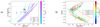 |
Fig. 4. Same as for Fig. 3, but for S34 and S3S4. |
| In the text | |
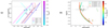 |
Fig. 5. Same as for Fig. 3, but for O34 and O3O4. |
| In the text | |
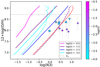 |
Fig. 6. Same as for Fig. 3a, but for N3. |
| In the text | |
|
Fig. 7. Comparison between the chemical abundances and U values introduced as inputs for the models (x-axis) with the estimations from HCM-IR when all lines plus [S III]λ33 μm are used (y-axis). For all plots we present Seyferts as blue circles and LINERs as green squares. The offsets are given using the median value (dashed line) and RMSE (dot-dashed lines). Bottom plots show the residuals from the offset and their distribution in a histogram (bottom-right plot). |
| In the text | |
|
Fig. 8. Comparison between the chemical abundances and U values introduced, obtained from the grid characterized by αOX = −0.8 and a 2% fraction of free electrons (x-axis) with models with αOX = −1.2 ((a), (c), and (e)) and models with 98% as stopping criteria ((b), (d), and (f)). For all plots we present Seyferts as blue circles, ULIRGs as green squares, LIRGs as magenta triangles, and LINERs as red stars. The offsets are given using the median value (dashed line) and RMSE (dot-dashed lines). Bottom plots show the residuals from the offset and their distribution in a histogram (bottom-right plot). |
| In the text | |
|
Fig. 9. N/O vs. O/H from IR estimations. The values for log(U) are given by the colorbar. |
| In the text | |
|
Fig. 10. Chemical abundances derived from optical emission lines in our sample of AGN. (a) Comparison between the chemical abundances derived with the calibration from Flury & Moran (2020; y-axis), denoted as FM20, and HCM (x-axis). (b) Comparison between the chemical abundances derived from the calibration from Carvalho et al. (2020; y-axis), denoted as FM20, with HCM (x-axis). For all plots we present Seyferts as blue circles, ULIRGs as green squares, LIRGs as magenta triangles, and LINERs as red stars. The offsets are given using the median value (dashed line) and RMSE (dot-dashed lines). Bottom plots show the residuals from the offset and their distribution in a histogram (bottom-right plot). |
| In the text | |
|
Fig. 11. N/O vs. O/H as derived from optical estimations. The log(U) values are given by the colorbar. |
| In the text | |
|
Fig. 12. Comparison between the chemical abundances and log(U) values obtained from optical emission lines using HCM (x-axis) and the corresponding estimations from IR lines using HCM-IR (y-axis). For all plots we present Seyferts as blue circles, ULIRGs as green squares, LIRGs as magenta triangles, and LINERs as red stars. The offsets are given using the median value (dashed line) and RMSE (dot-dashed lines). Bottom plots show the residuals from the offset and their distribution in a histogram (bottom-right plot). |
| In the text | |
|
Fig. 13. Discrepancies between the chemical abundance ratios (ΔX = Xopt − XIR) as a function of their ratios: (a) 12+log(O/H) and (c) log(N/O) both derived from IR emission lines with HCM-IR, and (b) 12+log(O/H) and (d) log(N/O) derived from optical emission lines with HCM. For all plots we present Seyferts as blue circles, ULIRGs as green squares, LIRGs as magenta triangles, and LINERs as red stars. |
| In the text | |
|
Fig. 14. Discrepancies between the chemical abundance ratios (ΔX = Xopt − XIR) as a function of the ionization parameter: (a) and (c) estimated from IR lines, (b) and (d) estimated from optical lines. |
| In the text | |
|
Fig. 15. Discrepancies between the chemical abundance ratios (ΔX = Xopt − XIR) as a function of the electronic density: (a) and (c) present electronic densities derived from [S III] lines, (b) and (d) present densities derived from [S II] lines. |
| In the text | |
Current usage metrics show cumulative count of Article Views (full-text article views including HTML views, PDF and ePub downloads, according to the available data) and Abstracts Views on Vision4Press platform.
Data correspond to usage on the plateform after 2015. The current usage metrics is available 48-96 hours after online publication and is updated daily on week days.
Initial download of the metrics may take a while.