| Issue |
A&A
Volume 685, May 2024
|
|
|---|---|---|
| Article Number | A168 | |
| Number of page(s) | 15 | |
| Section | Extragalactic astronomy | |
| DOI | https://doi.org/10.1051/0004-6361/202348318 | |
| Published online | 22 May 2024 | |
Chemical abundances and deviations from the solar S/O ratio in the gas-phase interstellar medium of galaxies based on infrared emission lines⋆
1
Instituto de Astrofísica de Andalucía (IAA-CSIC), Glorieta de la Astronomía s/n, 18008 Granada, Spain
e-mail: This email address is being protected from spambots. You need JavaScript enabled to view it.
2
Centro de Estudios de Física del Cosmos de Aragón (CEFCA), Unidad Asociada al CSIC, Plaza San Juan 1, 44001 Teruel, Spain
Received:
19
October
2023
Accepted:
4
March
2024
Abstract
Context. The infrared (IR) range is extremely useful in the context of chemical abundance studies of the gas-phase interstellar medium (ISM) due to the large variety of ionic species traced in this regime, the negligible effects from dust attenuation or temperature stratification, and the amount of data that has been and will be released in the coming years.
Aims. Taking advantage of available IR emission lines, we analysed the chemical content of the gas-phase ISM in a sample of 131 star-forming galaxies (SFGs) and 73 active galactic nuclei (AGNs). In particular, we derived the chemical content via their total oxygen abundance in combination with nitrogen and sulphur abundances, and with the ionisation parameter.
Methods. We used a new version of the code HII-CHI-MISTRY-IR v3.1, which allowed us to estimate log(N/O), 12+log(O/H), log(U) and, for the first time, 12+log(S/H) from IR emission lines, which can be applied to both SFGs and AGNs. We tested whether the estimates from this new version, which only considers sulphur lines for the derivation of sulphur abundances, are compatible with previous studies.
Results. While most of the SFGs and AGNs show solar log(N/O) abundances, we find a large spread in the log(S/O) relative abundances. Specifically, we find extremely low log(S/O) values (1/10 solar) in some SFGs and AGNs with solar-like oxygen abundances. This result warns against the use of optical and IR sulphur emission lines to estimate oxygen abundances when no prior estimation of log(S/O) is provided.
Key words: galaxies: abundances / galaxies: active / galaxies: ISM / galaxies: nuclei / infrared: ISM
Full Tables A.1–A.4 are available at the CDS via anonymous ftp to cdsarc.cds.unistra.fr (130.79.128.5) or via https://cdsarc.cds.unistra.fr/viz-bin/cat/J/A+A/685/A168
© The Authors 2024
 Open Access article, published by EDP Sciences, under the terms of the Creative Commons Attribution License (https://creativecommons.org/licenses/by/4.0), which permits unrestricted use, distribution, and reproduction in any medium, provided the original work is properly cited.
This article is published in open access under the Subscribe to Open model. This email address is being protected from spambots. You need JavaScript enabled to view it. to support open access publication.
1. Introduction
Emission lines measured in the gas phase of the interstellar medium (ISM) in galaxies are key to inferring their physical and chemical properties. Among these emission lines, collisionally excited lines (CELs) have been widely used for this purpose in several spectral ranges, such as in the optical (e.g., Lequeux et al. 1979; Garnett & Shields 1987; Contini & Viegas 2001; Pérez-Montero 2014; Curti et al. 2017), the ultraviolet (UV; e.g., Erb et al. 2010; Dors et al. 2014; Pérez-Montero & Amorín 2017), and the infrared (IR; e.g., Nagao et al. 2011; Pereira-Santaella et al. 2017; Peng et al. 2021; Fernández-Ontiveros et al. 2021; Pérez-Díaz et al. 2022). As the primordial ISM metal content after the Big Bang nucleosynthesis is well constrained (Cyburt et al. 2016), any subsequent deviation from these initial chemical conditions must be attributed to stellar nucleosynthesis, whose products are ejected into the ISM in the late stages of stellar evolution. Therefore, the analysis of the metal content of the ISM is fundamental to understanding the impact of dissipative baryonic processes in galaxy evolution.
Over the decades, several techniques based on CELs have been developed and improved to infer the metal content of the ISM in star-forming galaxies (SFGs; see Maiolino & Mannucci 2019, for a review on the topic). Moreover, in recent years, similar techniques have also started to be applied to the study of the chemical content of the ISM in the narrow line region (NLR) of active galactic nuclei (AGNs), accounting for the corresponding differences in the sources ionising the surrounding gas (e.g., Contini & Viegas 2001; Dors et al. 2015; Pérez-Montero et al. 2019; Pérez-Díaz et al. 2021).
Most of the studies devoted to the analysis of chemical abundances in the gas-phase ISM using CELs are focused on the oxygen (O) content (12+log(O/H)), for several reasons: (i) O is the most abundant metal by mass in the gas-phase ISM (∼55%, Peimbert et al. 2007), and is therefore a good proxy for the total metallicity (Z); and, (ii) its abundance can be derived more easily than other elements due to the presence of strong CELs in the optical, IR, and UV spectral ranges. Additionally, some authors have also analysed the nitrogen-to-oxygen abundance ratio (log(N/O); e.g., Vila-Costas & Edmunds 1993; Pérez-Montero & Contini 2009; Amorín et al. 2010; Andrews & Martini 2013; Peng et al. 2021; Fernández-Ontiveros et al. 2021; Pérez-Díaz et al. 2022). Nitrogen (N) can be produced by massive stars via a primary channel – leading to an almost constant N/O ratio – but also through a secondary channel in the high-metallicity regime, due to CNO cycles in intermediate-mass stars that eject it into the ISM after a certain time delay (e.g., Henry et al. 2000). Thus, the study of N/O using nitrogen emission lines can provide complementary information on the evolution of the chemical content of the ISM. While studies of N/O from both optical and IR emission lines can be performed, in the UV other secondary elements – such as carbon (C) – are studied instead, due to the presence of strong emission lines in this range, although it is also possible to study this by using optical recombination lines (e.g., Toribio san Cipriano et al. 2017; Méndez-Delgado et al. 2022), with the disadvantage that these emission lines are much fainter than CELs (Esteban et al. 2009).
So far, very few works have studied in a statistically significant sample of galaxies the sulphur (S) content in the gas-phase ISM. Instead, the assumption of an universal S/O ratio has been used to propose that sulphur emission lines are tracers of the total oxygen metallicity. For instance, Vilchez & Esteban (1996) were pioneers in defining the sulphur abundance parameter, S23:
![Mathematical equation: $$ \begin{aligned} \mathrm{S}_{23} = \frac{ {I} \left( \left[ \mathrm{{\text{ S}}{\small { {\text{ II}}}}} \right]\lambda \lambda 6717,6731 \right) + {I} \left( \left[ \mathrm{{\text{ S}}{\small { {\text{ III}}}}} \right] \lambda \lambda 9069,9532 \right) }{ {I} \left( \mathrm{H}_{\beta } \right) } \end{aligned} $$](/articles/aa/full_html/2024/05/aa48318-23/aa48318-23-eq1.gif) (1)
(1)
Later on, Díaz & Pérez-Montero (2000) provided the first calibration to directly estimate the oxygen content from S23, improving the determination of the chemical content of the gas-phase ISM, counteracting the ambiguity of the equivalent oxygen parameter, R23 (Pagel et al. 1979). As was shown by these authors, and after further improvements to the calibration of this estimator (Pérez-Montero & Díaz 2005), two advantages arise from using sulphur emission lines instead of oxygen (i.e., R23): (i), S23 is mainly single-valued in most of the metal abundance range; and, (ii) sulphur lines are less affected by extinction than oxygen emission lines, although [S III] lines at 9069 Å and 9531 Å can suffer from telluric absorptions (e.g., Noll et al. 2012).
However, the use of S23 to estimate 12+log(O/H) directly implies that the ratio between S and O (log(S/O)) remains constant. Indeed, while S and O are both produced in the nucleosynthesis of massive stars, their yields are expected to also behave similarly, supporting the previous idea of a constant S/O ratio. Unfortunately, this assumption has not been firmly established, and only a few works have analysed the sulphur content in the ISM (e.g., Kehrig et al. 2006; Pérez-Montero et al. 2006; Díaz et al. 2007; Berg et al. 2020; Díaz & Zamora 2022; Dors et al. 2023) as compared to the large number of studies on the oxygen content. Therefore, further observational constrains are required to validate the assumption of a universal solar S/O ratio. For instance, while Berg et al. (2020) show that most H II regions in their sample are consistent with a S/O solar ratio, Díaz & Zamora (2022) find strong deviations from that, especially in the low-metallicity regime (12+log(O/H) < 8.1). In this regard, it is important to note that at low metallicities a higher ionisation degree of the gas-phase ISM is expected, so higher ionic species (such as S+3) contribute more to the total budget of the sulphur content, and thus the uncertainty due to the application of the ionisation correction factor (ICF) to optical lines is higher. Moreover, Dors et al. (2023) also find a few sources among their AGN sample, with S/O ratios in some galaxies far from the solar value. Several attempts have been also made to directly calibrate the S23 parameter with the total sulphur abundance (Pérez-Montero et al. 2006; Díaz & Zamora 2022). However, the collisional nature of the lines involved in this parameter, which make them very dependent on the electron temperature, and thus on the overall metal content of the gas, implies an additional dependence on the assumed S/O ratio.
Nevertheless, the above-mentioned studies focus on the use of optical emission lines, leading to an inconclusive response as to whether these deviations originate intrinsically in the production of S and O, or due to a variety of effects with diverse origins such as dust attenuation, contamination from diffuse ionised gas (DIG), or the effects from the assumed ICFs, which severely affect the total sulphur abundances derived from the optical emission lines, as these do not cover the higher ionised S stages, such as S3+. In this regard, the study of IR emission lines opens a new avenue through which to determine sulphur abundances, both in SFGs and AGNs, with key advantages over optical tracers. First of all, due to the atomic transitions involved in the ionic radiative process, the IR emission lines are much less affected by the electron temperature, Te, avoiding problems due to stratification or temperature fluctuations (e.g., Peimbert 1967; Stasińska 2005; Méndez-Delgado et al. 2023; Jin et al. 2023). Secondly, the IR range allows the detection of highly ionised species such as S+3, which are important for a more accurate determination of total elemental abundances, especially in AGNs. Thirdly, IR emission lines are almost unaffected by dust obscuration. Fourthly, ancillary data from observatories such as the Infrared Space Observatory (ISO; covering the 2.4–197 μm range; Kessler et al. 1996), the Spitzer Space Observatory (5–39 μm; Werner et al. 2004), the Herschel Space Observatory (51–671 μm, Pilbratt et al. 2010), and the Stratospheric Observatory for Infrared Astronomy (SOFIA; covering the 50–205 μm range; Fischer et al. 2018), as well as brand-new missions such as the James Webb Space Telescope (JWST, which is covering the 4.9–28.9 μm range with the Mid-InfraRed Instrument MIRI, Rieke et al. 2015; Wright et al. 2015), and upcoming facilities such as the Mid-infrared Extremely large Telecope Imager and Spectrograph (METIS, covering the N-band centered at 10 μm, Brandl et al. 2021).
In this work, we compiled a sample of SFGs and AGNs with IR spectroscopic observations to derive their chemical abundances from the IR emission lines, following the methodology used in Fernández-Ontiveros et al. (2021) for SFGs and in Pérez-Díaz et al. (2022) for AGNs, which includes an independent estimation of log(N/O), 12+log(O/H) and 12+log(S/H). The paper is organised as follows. Section 2 provides information on the sample selection as well as on the methodology followed through this work. The main results of this study are shown in Sect. 3 and discussed in Sect. 4. Finally, we summarise our conclusion in Sect. 5.
2. Sample and methodology
For this work, we compiled one of the largest sample of galaxies with IR spectroscopic observations, combining catalogs from Spitzer, Herschel, Akari and SOFIA. In particular, we compiled the following catalogs: the dwarf galaxy sample from Cormier et al. (2015) observed with Spitzer and Herschel; the Infrared Database of Extragalactic Observables from Spitzer1 (IDEOS Hernán-Caballero et al. 2016; Spoon et al. 2022) from the Spitzer archive; the AGN and HII samples from Fernández-Ontiveros et al. (2016) and Spinoglio et al. (2022) combining Spitzer, Herschel, and SOFIA data; and the (U)LIRG catalog from Imanishi et al. (2010) observed with Akari.
2.1. Sample of star-forming galaxies
Our sample of SFGs is composed of objects from two main sources. The data of the first subsample were directly taken from Fernández-Ontiveros et al. (2021), where they compiled a sample of 65 galaxies (30 dwarf galaxies, 22 H II regions, and 13 (U)LIRGs) with IR spectroscopic observations showing star-formation dominated emission ([NeV]/[NeII] < 0.15). Additionally, we compiled another sample of galaxies from the IDEOS catalog (Hernán-Caballero et al. 2016; Spoon et al. 2022). As is described in Pérez-Díaz et al. (2024), the sample consists of 66 ultra-luminous infrared galaxies (ULIRGs) showing star-forming dominated activity from both their [NeV]/[Ne II] ratio (< 0.15) and from the equivalent width of the PAH feature at 6.2 μm (EQW(PAH6.2 μm) > 0.06 μm). While for this last sample we compiled IR emission lines from [SIV]λ10 μm to [S III]λ33 μm from IDEOS (Spoon et al. 2022) and measurements of HIλ4.05 μm from Akari/IRC observations (2.5–5 μm, Imanishi et al. 2010), only the first sample from Fernández-Ontiveros et al. (2021) presents measurements from far-IR emission lines such as [O III]λ52 μm, [N III]λ57 μm, and [O III]λ88 μm, which are key to estimating N/O.
2.2. Sample of active galactic nuclei
We compiled our AGN sample from Pérez-Díaz et al. (2022), who analysed 58 AGNs with available IR spectroscopic observations, including 17 Seyfert 1 nuclei (Sy1), 14 Seyfert nuclei with hidden broad lines in the polarised spectrum (Sy1h), 12 Seyfert 2 nuclei (Sy2), 12 (U)LIRGs, and three low-ionisation nuclear emission-line regions (LINERs). Additionally, we included 15 quasars from the IDEOS catalog (up to redshift ∼0.74), for which we also added measurements, when possible, of the hydrogen recombination line, the HI Brackett α line, from their Akari/IRC observations (2.5–5 μm, Imanishi et al. 2010). We measured fluxes in the HIλ4.05 μm line by fitting the restframe [3.8–4.3 μm] range with a model that assumes a second-order polynomial for the continuum and a Gaussian profile for the line, with the line width corresponding to the instrumental resolution of the Akari or Spitzer/IRS spectrum at that wavelength2. Both samples show strong AGN emission, as is shown by their [NeV]/[NeII] (≫0.15) ratio.
2.3. HII-CHI-MISTRY-IR
To derive chemical abundances from the IR emission lines in our sample, we used the code HII-CHI-MISTRY-IR (hereinafter, HCM-IR) v3.1, originally developed by Pérez-Montero (2014) for optical emission lines and later extended to IR emission lines by Fernández-Ontiveros et al. (2021) for SFGs and Pérez-Díaz et al. (2022) for AGNs. This code basically performs a Bayesian-like comparison between a set of observed emission-line flux ratios sensitive to quantities such as the total oxygen abundance, the nitrogen-to-oxygen ratio, or the ionisation parameter, with the predictions from large grids of photoionisation models to provide the most probable values of these quantities and their corresponding uncertainties.
Version 3.1 of the code for the IR3 presents two new features in relation to previous versions:
-
The code now accepts as input the argon emission lines ([Ar II]λ7 μm, [Ar III]λ9 μm, [Ar V]λ8 μm, and [Ar V]λ13 μm), which are used to construct estimators of metallicity and excitation, analogous to those based on neon emission lines already used in previous versions; that is, Ne23 and Ne2Ne3 for SFGs (Fernández-Ontiveros et al. 2021):
![Mathematical equation: $$ \begin{aligned}&\log \left( \mathrm{Ne23} \right) = \log \left( \frac{ {I} \left( \left[ \mathrm{{\text{ Ne}}{\small { {\text{ II}}}}} \right] _{12\,\upmu \mathrm{m}} \right) + {I} \left( \left[ \mathrm{{\text{ Ne}}{\small { {\text{ III}}}}} \right] _{\rm 15\,\upmu m} \right) }{ {I} \left( \mathrm{{\text{ H}}{\small { {\text{ I}}}}} _{i} \right) } \right), \end{aligned} $$](/articles/aa/full_html/2024/05/aa48318-23/aa48318-23-eq2.gif) (2)
(2)![Mathematical equation: $$ \begin{aligned}&\log \left( \mathrm{Ne2Ne3} \right) = \log \left( \frac{ {I} \left( \left[ \mathrm{{\text{ Ne}}{\small { {\text{ II}}}}} \right] _{\rm 12\,\upmu m} \right) }{ {I} \left( \left[ \mathrm{{\text{ Ne}}{\small { {\text{ III}}}}} \right] _{\rm 15\,\upmu m} \right) } \right), \end{aligned} $$](/articles/aa/full_html/2024/05/aa48318-23/aa48318-23-eq3.gif) (3)
(3)and Ne235 and Ne23Ne5 for AGNs (Pérez-Díaz et al. 2022):
![Mathematical equation: $$ \begin{aligned}&\log \left( \mathrm{Ne235} \right) = \log \left( \frac{ {I} \left( \left[ \mathrm{{\text{ Ne}}{\small { {\text{ II}}}}} \right] _{\rm 12\,\upmu m} \right) + {I} \left( \left[ \mathrm{{\text{ Ne}}{\small { {\text{ III}}}}} \right] _{\rm 15\,\upmu m} \right) }{ {I} \left( \mathrm{{\text{ H}}{\small { {\text{ I}}}}} _{i} \right) } + \right. \nonumber \\&\qquad \qquad \qquad + \left. \frac{ {I} \left( \left[ \mathrm{{\text{ Ne}}{\small { {\text{ V}}}}} \right] _{\rm 14\,\upmu m} \right) + {I} \left( \left[ \mathrm{{\text{ Ne}}{\small { {\text{ V}}}}} \right] _{\rm 24\,\upmu m} \right) }{ {I} \left( \mathrm{{\text{ H}}{\small { {\text{ I}}}}} _{i} \right) } \right), \end{aligned} $$](/articles/aa/full_html/2024/05/aa48318-23/aa48318-23-eq4.gif) (4)
(4)![Mathematical equation: $$ \begin{aligned}&\log \left( \mathrm{Ne23Ne5} \right) = \log \left( \frac{ {I} \left( \left[ \mathrm{{\text{ Ne}}{\small { {\text{ II}}}}} \right] _{\rm 12\,\upmu m} \right) + {I} \left( \left[ \mathrm{{\text{ Ne}}{\small { {\text{ III}}}}} \right] _{\rm 15\,\upmu m} \right) }{ {I} \left( \left[ \mathrm{{\text{ Ne}}{\small { {\text{ V}}}}} \right] _{\rm 14\,\upmu m} \right) + {I} \left( \left[ \mathrm{{\text{ Ne}}{\small { {\text{ V}}}}} \right] _{\rm 24\,\upmu m} \right) } \right). \end{aligned} $$](/articles/aa/full_html/2024/05/aa48318-23/aa48318-23-eq5.gif) (5)
(5)Following this approach, the new observables based on these IR argon lines can be defined as
![Mathematical equation: $$ \begin{aligned}&\log \left( \mathrm{Ar23} \right) = \log \left( \frac{ {I} \left( \left[ \mathrm{{\text{ Ar}}{\small { {\text{ II}}}}} \right] _{\rm 7\,\upmu m} \right) + {I} \left( \left[ \mathrm{{\text{ Ar}}{\small { {\text{ III}}}}} \right] _{\rm 9\,\upmu m} \right) }{ {I} \left( \mathrm{{\text{ H}}{\small { {\text{ I}}}}} _{i} \right) } \right), \end{aligned} $$](/articles/aa/full_html/2024/05/aa48318-23/aa48318-23-eq6.gif) (6)
(6)![Mathematical equation: $$ \begin{aligned}&\log \left( \mathrm{Ar2Ar3} \right) = \log \left( \frac{ {I} \left( \left[ \mathrm{{\text{ Ar}}{\small { {\text{ II}}}}} \right] _{\rm 7\,\upmu m} \right) }{ {I} \left( \left[ \mathrm{{\text{ Ar}}{\small { {\text{ III}}}}} \right] _{\rm 9\,\upmu m} \right) } \right), \end{aligned} $$](/articles/aa/full_html/2024/05/aa48318-23/aa48318-23-eq7.gif) (7)
(7)![Mathematical equation: $$ \begin{aligned}&\log \left( \mathrm{Ar235} \right) = \log \left( \frac{ {I} \left( \left[ \mathrm{{\text{ Ar}}{\small { {\text{ II}}}}} \right] _{\rm 7\,\upmu m} \right) + {I} \left( \left[ \mathrm{{\text{ Ar}}{\small { {\text{ III}}}}} \right] _{\rm 9\,\upmu m} \right) }{ {I} \left( \mathrm{{\text{ H}}{\small { {\text{ I}}}}} _{i} \right) } + \right. \nonumber \\&\qquad \qquad \qquad + \left. \frac{ {I} \left( \left[ \mathrm{{\text{ Ar}}{\small { {\text{ V}}}}} \right] _{\rm 8\,\upmu m} \right) + {I} \left( \left[ \mathrm{{\text{ Ar}}{\small { {\text{ V}}}}} \right] _{\rm 13\,\upmu m} \right) }{ {I} \left( \mathrm{{\text{ H}}{\small { {\text{ I}}}}} _{i} \right) } \right), \end{aligned} $$](/articles/aa/full_html/2024/05/aa48318-23/aa48318-23-eq8.gif) (8)
(8)![Mathematical equation: $$ \begin{aligned}&\log \left( \mathrm{Ar23Ar5} \right) = \log \left( \frac{ {I} \left( \left[ \mathrm{{\text{ Ar}}{\small { {\text{ II}}}}} \right] _{\rm 7\,\upmu m} \right) + {I} \left( \left[ \mathrm{{\text{ Ar}}{\small { {\text{ III}}}}} \right] _{\rm 9\,\upmu m} \right) }{ {I} \left( \left[ \mathrm{{\text{ Ar}}{\small { {\text{ V}}}}} \right] _{\rm 8\,\upmu m} \right) + {I} \left( \left[ \mathrm{{\text{ Ar}}{\small { {\text{ V}}}}} \right] _{\rm 13\,\upmu m} \right) } \right), \end{aligned} $$](/articles/aa/full_html/2024/05/aa48318-23/aa48318-23-eq9.gif) (9)
(9)with H Ii being one of the hydrogen lines that the code can take as input. The performance of these estimators is shown in Fig. 1 in comparison with their neon analogues. Argon emission lines offer a great opportunity for chemical abundance studies with JWST data, since they are located in a narrow IR window [7 μm,13 μm], argon is a non-depleted element whose nucleosynthesis leads to a yield similar to that for oxygen, and they include transitions from highly ionised species, which helps to disentangle the power of the ionising source.
-
After the iteration4 performed by the code to constrain N/O, and parallel to the second iteration performed to estimate 12+log(O/H) and the ionisation parameter log(U), the code now performs a new iteration to estimate 12+log(S/H). This is done using the estimators S34 and S3S4 (Fernández-Ontiveros et al. 2021; Pérez-Díaz et al. 2022), based on sulphur lines, without assuming the results from the oxygen or the ionisation estimations. In this way, the estimators based on sulphur emission lines (S34 and S3S4) are no longer used for the estimation of 12+log(O/H) and log(U) and, consequently, sulphur and oxygen abundances are derived independently from each other’s estimations.
![Mathematical equation: $$ \begin{aligned}&\log \left( \mathrm{S34} \right) = \log \left( \frac{ {I} \left( \left[ \mathrm{{\text{ S}}{\small { {\text{ III}}}}} \right] _{\rm 18\,\upmu m} \right) + {I} \left( \left[ \mathrm{{\text{ S}}{\small { {\text{ III}}}}} \right] _{33\,\upmu m} \right) }{ {I} \left( \mathrm{{\text{ H}}{\small { {\text{ I}}}}} _{i} \right) } + \right.\nonumber \\&\qquad \qquad \qquad + \left. \frac{ {I} \left( \left[ \mathrm{{\text{ S}}{\small { {\text{ IV}}}}} \right] _{\rm 10\,\upmu m} \right) }{ {I} \left( \mathrm{{\text{ H}}{\small { {\text{ I}}}}} _{i} \right) } \right), \end{aligned} $$](/articles/aa/full_html/2024/05/aa48318-23/aa48318-23-eq10.gif) (10)
(10)![Mathematical equation: $$ \begin{aligned}&\log \left( \mathrm{S3S4} \right) = \log \left( \frac{ {I} \left( \left[ \mathrm{{\text{ S}}{\small { {\text{ III}}}}} \right] _{\rm 18\,\upmu m} \right) + {I} \left( \left[ \mathrm{{\text{ S}}{\small { {\text{ III}}}}} \right] _{\rm 33\,\upmu m} \right) }{ {I} \left( \left[ \mathrm{{\text{ S}}{\small { {\text{ IV}}}}} \right] _{\rm 10\,\upmu m} \right) } \right). \end{aligned} $$](/articles/aa/full_html/2024/05/aa48318-23/aa48318-23-eq11.gif) (11)
(11)Following the prescription by Pérez-Díaz et al. (2022), the emission line [S III]λ33μm is only used for SFGs. The performance of these estimators is shown in Fig. 2. It is relevant to emphasise the importance of IR emission lines in estimating sulphur abundances. As is shown in Fig. 3, S/O has little dependence on the behaviour of the estimators, as the intensity of IR emission lines mainly depends on the ionic abundance. However, this is no longer the case for optical lines, as they also depend on temperature, which translates into a dependence on the metallicity. Hence, estimators for sulphur based on optical emission lines (e.g. S23 Eq. (1)) are much more affected by the S/O assumed for the models.
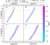 |
Fig. 1. Performance of estimators based on neon ((a) and (c)) and argon ((b) and (d)) emission lines. Panels a and b show the behaviour of estimators Ne23 and Ar23 for SFG models, with plus symbols presenting values from our SFG sample. Panels c and d show the behaviour of estimators Ne235 and Ar235 for AGNs. SF models presented by Fernández-Ontiveros et al. (2021) are shown as dashed lines, while AGN models presented by Pérez-Díaz et al. (2022) are shown as continuous lines. |
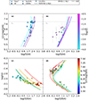 |
Fig. 2. Performance of estimators based on sulphur emission lines. Panels a and c show the performance of S34 for 12+log(S/H) and S3S4 for log(U), respectively, in the case of SFGs. Panels b and d show the performance of the same estimators for AGNs. Models are shown following the same notation as in Fig. 1. |
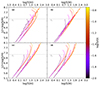 |
Fig. 3. Performance of estimator S34 based on sulphur emission lines for models with S/O that is not fixed. Panel a shows models for a fixed value of the ionisation parameter log(U) = − 1.5, panel b shows models for log(U) = − 2.0, panel c models with log(U) = − 3.0, and panel d those with log(U) = − 3.5. Models are shown following the same notation as in Fig. 1. |
As is shown in Fig. 4, these new improvements in the code do not significantly change the results obtained with previous versions, but we do obtain more information, as now 12+log(S/H) is independently estimated. We notice that some AGNs seem to present slightly higher abundances when sulphur emission lines are no longer used in the oxygen estimation, which implies that S lines favour lower abundances (see Sect. 3).
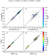 |
Fig. 4. Comparison between the outputs from HCM v3.01 (x-axis) and HCM v3.1 (y-axis). Panels a and b show a comparison of SFGs and AGNs, respectively, with 12+log(O/H). Panels c and d show a comparison of SFGs and AGNs, respectively, with log(U). |
3. Results
In this section, we present an analysis of the chemical abundances obtained after applying HCM-IR to the selected samples presented in Sect. 2. The statistics of these results are shown in Table 1.
Statistics of the chemical abundances and log(U) values derived from HCM-IR for our sample of galaxies.
3.1. Nitrogen-to-oxygen abundance ratios
HCM-IR performs a first independent iteration to estimate log(N/O). Since both the IR observables (i.e., N3O3 ≡ [N III]57 μm/[O III]52 μm) and the procedure followed to determine N/O remain unchanged in this version, no significant difference is found in the log(N/O) distribution derived for the SFG and AGN samples when compared to studies based on previous versions of the code. In the case of SFGs, the median value of log(N/O) ∼ −0.9 is close to the solar ratio, in agreement with Fernández-Ontiveros et al. (2021). Regarding AGNs, the distribution is almost identical to that reported by Pérez-Díaz et al. (2022). Moreover, as IDEOS measurements do not cover the far-IR emission lines, essential to estimating log(N/O) (Peng et al. 2021; Fernández-Ontiveros et al. 2021; Pérez-Díaz et al. 2022), the number of N/O measurements has not increased with respect to previous works.
Figure 5 shows that the distribution of the IR-based log(N/O) versus the 12+log(O/H) values obtained for our sample deviates from the abundances obtained for local SFGs using optical lines (Pérez-Montero & Contini 2009; Andrews & Martini 2013; Pérez-Montero 2014). Our IR-based abundances cluster around the solar N/O ratio and do not show a trend with O/H. While this result seems to contradict previous studies (e.g., Spinoglio et al. 2022), we must bear in mind the low number of AGNs with N/O estimations. It is also important to note that while SFGs present values of N/O that spread from sub-solar to over-solar ratios, AGNs present either solar or slightly over-solar N/O ratios.
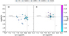 |
Fig. 5. N/O vs. O/H as derived from infrared emission lines for SFGs (a) and AGNs (b). The log(U) values are given by the colour bar. |
This result is also reported for the abundances of SFGs as derived from their IR lines (Fernández-Ontiveros et al. 2021) and for AGNs (Pérez-Díaz et al. 2022), in both cases with calculations based on HCM-IR. Since 12+log(O/H) is now obtained without considering the IR sulphur lines, in contrast to previous studies, we conclude that these behaviours on the N/O–O/H diagram persist even when the information is solely obtained from O, Ne, and Ar emission lines.
3.2. Sulphur and oxygen abundances
The analysis of the total oxygen abundance in our sample of SFGs is in overall agreement with Fernández-Ontiveros et al. (2021). We find the lowest 12+log(O/H) average values in dwarf galaxies (12+log(O/H) ∼ 8.0), with sub-solar abundances for (U)LIRGs (12+log(O/H) ∼ 8.5) and the highest values for HII regions (12+log(O/H) ∼ 8.7). Nevertheless, our larger (ULIRG) sample presents a slightly higher median oxygen abundance when compared to the smaller sample of 12 objects in Fernández-Ontiveros et al. (2021). The agreement with previous determinations implies that the independent estimation of S in the last version of HCM-IR does not significantly change the abundances of O and N, as in the Bayesian-like procedure sulphur estimators are weighted among many others, reducing any possible bias. Regarding the derived average sulphur content, 12+log(S/H), in our sample of SFGs, we obtained a similar behaviour to that of oxygen, the lowest value being found in dwarfs (12+log(S/H) ∼ 6.3), followed by (U)LIRGs (12+log(S/H) ∼ 6.8) and HII regions (12+log(S/H) ∼ 7.1).
The 12+log(O/H) values obtained for AGNs are also consistent with previous studies (Pérez-Díaz et al. 2022), as there is not a significant increase in the oxygen content for high-ionisation (Seyfert) AGNs. This is supported by the larger statistics after including the AGNs from IDEOS. Hence, we can conclude that, in terms of chemical content, the samples from IDEOS and from Pérez-Díaz et al. (2022) are both similar. Overall, the whole AGN sample presents similar median values for both 12+log(O/H) ∼ 8.25 and 12+log(S/H) ∼ 6.5 for all considered subtypes (Seyferts, LINERs, and (U)LIRGs).
Finally, we also explored the relation between the ionisation parameter, log(U), and the derived chemical abundances. Theoretically, if massive stars are the sources of ionisation, an anti-correlation between metallicity and ionisation is expected as a consequence of: (1) stars becoming cooler as a result of wind and enhanced line blanketing (Massey et al. 2005); and, (2) an increase in the stellar atmosphere content leading to higher photon scattering, which later translates into a more efficient conversion of the luminosity energy into the mechanical energy in winds (Dopita et al. 2006). As is presented in Fig. 6, we did obtain an anti-correlation for SFGs that is stronger for oxygen (the Pearson coefficient correlation is r ∼ −0.98) than for sulphur (the Pearson coefficient correlation is r ∼ −0.8). When analysing AGNs, we do not obtain any relation between metallicity and the ionisation parameter, in agreement with previous studies (e.g., Pérez-Montero et al. 2019; Pérez-Díaz et al. 2021, 2022). Moreover, the lack of correlation between U and O/H (and S/H) is obtained in galaxies characterised by high ionisation parameters (log(U) > − 2.5 such as Seyferts) but also in AGN-dominated (U)LIRGs with low ionisation parameters (log(U) < − 2.5), as is shown in Fig. 7.
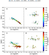 |
Fig. 6. Variation in the ionisation parameter, log(U), as a function of the chemical abundance ratios, 12+log(O/H) (panels a and b) and 12+log(S/H) (panels c and d). Panels a and c show results from SFGs, while panels b and d present AGNs. |
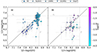 |
Fig. 7. S/H vs. O/H as derived from infrared emission lines for SFGs (a) and AGNs (b). The log(U) values are given by the colour bar. The solid line represents the solar proportion. We notice in panel a that (U)LIRGs with high S/H values near the lowest values for O/H are the same galaxies that are experiencing the deep-diving phase reported by Pérez-Díaz et al. (2024). |
3.3. Sulphur-to-oxygen abundance ratios
The median log(S/O) values obtained for our samples of SFGs (−1.89) and AGNs (−1.87) are lower than the solar ratio, log(S/O)⊙ = −1.57 (Asplund et al. 2009). From Fig. 7 we conclude that, although the median values deviate by a factor of 0.3 dex from the solar ratio, higher offsets are found in many of the (U)LIRGs (in our sample, dominated by either star-forming or AGN activity), as their sulphur abundances are significantly lower than the expected values of their corresponding oxygen estimations.
First of all, we explored the possibility that these deviations in the log(S/O) chemical abundance ratio could be caused by uncertainties in the measurement of the [S IV]λ10 μm emission line. Among these, the flux of this line could be affected as a consequence of the presence of a silicate feature detected in the 10–12.58 μm range (Spoon et al. 2022). From Fig. 8 we can conclude that the silicate strength does not play any role in the estimated values of log(S/O). However, we must bear in mind that in galaxies dominated by AGN activity the silicate strength provides information on the extinction that is affecting the continuum emission, whereas the line emission can come from more extended parts.
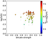 |
Fig. 8. S/O vs. the silicate strength in the 10–12.58 μm range as measured in IDEOS (Spoon et al. 2022). The colour bar shows the values for the 12+log(S/H) chemical abundance. |
To further explore the above-reported deviations in the chemical abundance ratio, log(S/O), of our sample, we studied its behaviour as a function of the oxygen abundance. As is shown in Fig. 9, the deviations in log(S/O) are found in either the low-metallicity regime (12+log(O/H) < 8.0), as is the case for SFGs, or in the high-metallicity regime (12+log(O/H) > 8.4), for both SFGs and AGNs. In the two metallicity regimes, (U)LIRGs are the galaxies driving these high deviations.
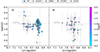 |
Fig. 9. S/O vs. O/H as derived from the infrared emission lines for SFGs (a) and AGNs (b). The log(U) values are given by the colour bar. Again, the (U)LIRGs that show the highest S/O ratios are the same galaxies that are undergoing the deep-diving phase reported by Pérez-Díaz et al. (2024). |
In the specific case of SFGs, we explored if these deviations correlate with other physical quantities such as the stellar mass (M*) or the star formation rate (SFR), as galaxy mass assembly is known to play an important role in the chemical enrichment of galaxies (Curti et al. 2017; Maiolino & Mannucci 2019), materialised in the well-known mass–metallicity relation (MZR, Lequeux et al. 1979; Tremonti et al. 2004; Andrews & Martini 2013). Although this relation is regulated by many processes such as the galactic environment (Peng & Maiolino 2014), secular evolution (Somerville & Davé 2015), star formation, and AGN feedback (Blanc et al. 2019; Thomas et al. 2019) or stellar age (Duarte Puertas et al. 2022), we only analysed those quantities that are explicitly involved in this connection between chemical enrichment and galaxy mass assembly: M* (Lequeux et al. 1979; Tremonti et al. 2004) and SFR (SFR, Mannucci et al. 2010; Curti et al. 2017).
Figure 10 shows that deviations from the solar ratio log(S/O)⊙ ∼ −1.57 are observed mostly in those galaxies with high M* (> 1011 M⊙) and a high SFR (> 90 M⊙ yr−1).
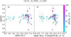 |
Fig. 10. (a) S/O vs. M*. (b) S/O vs. M* corrected from SFR, as proposed by Curti et al. (2017). The SFR values are given by the colour bar. |
4. Discussion
4.1. Information from sulphur emission lines
Unlike previous analyses of chemical abundances of the gas phase using IR lines, which assume a constant and universal S/O ratio, our work avoids S emission lines – namely [S IV] λ10 μm, [S III]λ18 μm, and [S III]λ33 μm – in estimating 12+log(O/H). Instead, the sulphur lines are used in this work to estimate 12+log(S/H) independently. Given the quantity and variety of other emission lines observed in the IR range (Ne, Ar, and O), sulphur emission lines do not play a critical role in the estimation of the oxygen abundance, as is evidenced by the high consistency between our results and previous studies using all of the lines (see Fig. 4).
While IR emission lines are extremely useful due to the fact that they are much less affected by temperature or dust extinction, their dependence on density should be taken into account. Far-IR emission lines present low critical densities (e.g., Pérez-Díaz et al. 2022), which implies that their fluxes can be affected even for the average conditions of the ISM in both SFGs (ne ∼ 100 cm−3) and AGNs (ne ∼ 500 cm−3). This is not the case for IR sulphur emission lines, as their critical densities (nc([S IV]10 μm)∼5.6 × 104 cm−3, nc([S III]18 μm)∼1.2 × 104 cm−3, and nc([S III]33 μm)∼1417 cm−3; Pérez-Díaz et al. 2022) are well above such conditions of the ISM.
Furthermore, as the derivation of chemical abundances based on the IR range also involves intermediate and highly ionised species (S2+, S3+), the influence from DIG (Reynolds 1985; Domgorgen & Mathis 1994; Galarza et al. 1999; Zurita et al. 2000; Haffner et al. 2009), whose contribution is only relevant for low-excitation lines, is expected to be negligible in the abundance calculation. In addition, the detection of high-excitation IR lines is also extremely important in the case of AGNs, especially in high-luminosity AGNs such as Seyferts or quasars, since highly ionised species are needed to correctly trace the chemical content of the gas-phase ISM, and these ions produce emission lines that are easily detected in the IR range.
4.2. Deviations from the S/O solar ratio
Our analysis of the chemical abundance ratio log(S/O) in the selected sample, calculated from the independent estimation of sulphur and oxygen abundances, reveals that many galaxies present values close to the solar ratio. As a matter of fact, about 70% of our sample of SFGs are within 0.2 dex of the solar ratio. However, this value drops to 44% when AGNs are considered. Focusing on the galaxies whose S/O ratio clearly deviates from the solar proportion (> 0.3 dex), we find that 53% of the AGNs and 17% of the SFGs present such large deviations.
Regarding the different subtypes of galaxies, (U)LIRGs exhibit the greatest deviations (see Fig. 7). Specifically, we find that (U)LIRGs with an oxygen content close to the solar value (12+log(O/H)⊙ ∼ 8.69) show a spread in S/O ratios of more than an order of magnitude (from −1.2 to −2.3), suggesting a strong variation in the sulphur content of galaxies with similar stellar masses, M* ∼ 1011 M⊙, and oxygen abundances, 12+log(O/H) ∼ 8.6 (see Fig. 10).
Among the (U)LIRGs that deviate from the solar log(S/O) ratio are those with very low abundances (12+log(O/H) < 8.2) compared to other galaxies of the same type. These (U)LIRGs possibly undergo a large excursion or deep dive beneath the MZR due to massive infalls of metal-poor gas (Pérez-Díaz et al. 2024). According to our results, sulphur abundances are higher in these objects, leading to over-solar log(S/O) > −1.2 ratios. This behaviour is similar to that reported by several authors using optical lines for different SFG samples (Diaz et al. 1991; Pilyugin et al. 2006; Díaz & Zamora 2022).
Diverse mechanisms able to drive the observed log(S/O) deviation in SFGs have been proposed, including: (1) changes in the initial mass function enhancing the formation of stars with masses between 12 M⊙ and 20 M⊙, which are the major producers of S via burning of O and Si (Díaz & Zamora 2022); and, (2) metal enrichment from Type Ia supernovae increasing the sulphur yield (Iwamoto et al. 1999). The first scenario could be favoured in the extreme star formation conditions that characterise deep-diving (U)LIRGs, as larger SFRs help to increase the number of stars with M > 10 M⊙. Moreover, if (U)LIRGs have experienced a change in their IMF, which has not been reported yet, then this effect could be amplified. On the other hand, the second mechanism proposed could be important in galaxies with strong outflows; for instance, Pérez-Díaz et al. (2024) discuss how strong feedback from the extreme episode of star formation is required for (U)LIRGs to end their deep-diving phase.
However, as is shown in Fig. 10, these deviations found in massive galaxies are not always associated with an increase in S, as we also observed extremely low log(S/O) abundances in similar conditions. Moreover, these scenarios do not explain why there is such a strong variation in the sulphur content of galaxies with similar oxygen abundances and stellar properties such as mass or the SFR. Another possible mechanism that could explain these lower abundances of S/H might be related to the formation of ice and dust grains that capture S in the most dense cores of molecular clouds (Hily-Blant 2022). Indeed, recent studies show that sulphur abundances in these cold, dense clouds are much lower than those reported in the ionised ISM (e.g., Fuente et al. 2023), and these cold regions can be traced by IR emission lines, while they remain unobserved from optical spectroscopy. Nevertheless, we cannot explore this scenario with the current IR data.
Active galactic nuclei show an analogous behaviour, with S/O abundances spread over a wide range for galaxies characterised by similar oxygen abundances. This was also reported by Dors et al. (2023) using optical emission lines; however, the information from S3+ – which plays an important role in deriving the total S abundance in the case of strong AGNs such as Seyferts – was missing. As in the case of SFGs, it is unclear whether the proposed scenarios of chemical enrichment from both stellar nucleosynthesis and feedback might explain the observed deviations. Nevertheless, we report the absence of AGNs with clear over-solar log(S/O) ratios, unlike deep-diving (U)LIRGs, implying either that galaxies classified as AGNs in our sample cannot meet the conditions to present such values, or that there is an observational bias towards objects with solar to sub-solar log(S/O) ratios.
In the near future, analysis of spatially resolved spectroscopic observations in the IR range for both SFGs and AGNs will shed light to better disentangle if the mechanisms proposed to explain the observed S/O variation are the same in both types of objects.
4.3. The role of electron density
The emissivities of the IR emission lines are significantly less dependent on temperature when compared with the optical transitions (e.g., Fernández-Ontiveros et al. 2021). However, the former are more affected by the electron density (ne) due to the lower critical densities (nc) of the IR transitions – that is, the density at which collisional de-excitations equal radiative transitions. For instance, [O III]88 μm has nc = 501 cm−3, whereas [O III]5007 Å has 6.9 × 105 cm−3. As is shown in Pérez-Díaz et al. (2022), most of the IR emission lines used in this work have nc well above the expected densities in SFGs (∼100 cm−3) and AGNs (∼500 cm−3), and therefore effects from the density conditions of the ISM are not critical for chemical abundance estimations. Additionally, HCM-IR (Fernández-Ontiveros et al. 2021; Pérez-Díaz et al. 2022) takes into account this information in the calculations and uses only those IR transitions whose nc are above the expected densities for the ionised ISM in each case. Nevertheless, to test the robustness of the S/O relative abundances obtained, we investigate in this section a possible dependency on the gas density.
For this purpose, we evaluated two ratios that are extremely sensitive to ne: [S III]33 μm/[S III]18 μm and [Ne V]24 μm/[Ne V]14 μm. The former is used to trace densities in SFGs, because it is the only available set of emission lines from the same ionic species in the mid-IR. The latter is used to measure densities in AGNs, as this ratio involves a highly ionised ion, thus avoiding possible contamination from star formation activity. In Fig. 11 we present the log(S/O) values as a function of these two emission-line ratios.
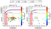 |
Fig. 11. Dependence of S/O on electron density. Panels a and c show the theoretical behaviour of the emission-line ratios, [S III]33 μm/[S III]18 μm and [Ne V]24 μm/[Ne V]14 μm, respectively, as a function of density for different values of the electron temperature, as computed by PYNEB (Luridiana et al. 2015). Panel b shows the behaviour of log(S/O) as a function of [S III]33 μm/[S III]18 μm for SFGs. Panel d shows the behaviour of log(S/O) as a function of [Ne V]24 μm/[Ne V]14 μm for AGNs. The colour bar shows the values of 12+log(S/H) for both samples. Critical densities were computed assuming Te = 10 000 K and are those associated with the emission line with the lowest value. |
The lack of correlation between log(S/O) and ne is shown in Fig. 11, suggesting that density variations are not causing the deviations from the solar ratio. A few SFGs (five) and AGNs (three) present densities that are compatible within the errors with the critical density regime (ne > nc), although the density uncertainties in all cases are compatible with lower values. Analysing the statistics for each sample, we find that SFGs and AGNs present median values of ne ∼ 200 cm−3 and ∼1000 cm−3, respectively, adopting an electron temperature of Te = 104 K. Nevertheless, we note that, given the uncertainties in the emission-line ratios involved, these results are still compatible with the typical ISM densities in each case.
On the other hand, there are some considerations that may impact the determination of electron densities. For instance, it has been probed that planetary nebulae present density inhomogeneities across the gas-phase ISM (e.g., Seaton & Osterbrock 1957; Flower 1969; Harrington 1969; Péquignot et al. 1978; Rubin 1989). Additionally, the action of shocks in the ISM might also induce variations in the density distribution (e.g., Dopita 1976, 1977; Dopita et al. 1977; Contini & Aldrovandi 1983; Aldrovandi & Contini 1985). While these effects can play an important role in the determination of the electron temperature, Te, for a direct estimation of chemical abundances using CELs, HCM-IR does not make any prior estimation of Te. Pérez-Montero et al. (2019) show that a variation in the electron density by a factor of four has a negligible effect on the chemical abundances derived using HCM. In the case of IR estimators, such as S34, Ne23, or Ne235, only remarkable differences (higher than 0.3 dex) are found when the densities are changed from 100 cm−3 for SFGs and 500 cm−3 for AGNs to 10 000 cm−3 in both cases, according to photoionisation models computed with CLOUDY v17 (Ferland et al. 2017). This value is well above the critical density for most of the IR emission lines considered, and there are no galaxies in this regime in our sample of SFGs and AGNs, as is shown in Fig. 11. Therefore, we conclude that the density conditions have no significant impact on the chemical abundances of 12+log(S/H) and 12+log(O/H) estimated in this work.
Finally, we note that a few SFGs and AGNs show values above the expected ratio in the low-density regime (i.e., ne → 0). Nevertheless, the deviations from the log(S/O) solar ratio are also found in the density regime between 100 cm−3 and 1000 cm−3, supporting the idea that these differences are not driven by variations in the gas density, but are instead intrinsic to the chemical composition of the ISM.
5. Conclusions
In this work we performed, for the first time, a systematic analysis of the chemical abundances estimated from IR emission lines in a sample of galaxies including both SFGs and AGNs, providing an independent estimation of the oxygen, nitrogen, and sulphur abundances for the widest sample of galaxies with IR spectroscopic observations, combining Spitzer, Herschel, AKARI, and SOFIA data. When comparing our results with previous studies of chemical abundances from IR emission lines, we find an agreement in the estimated oxygen and nitrogen abundances.
While most of the galaxies in the sample are characterised by a solar log(S/O) ratio, we report that galaxies with low to solar oxygen abundances present large deviations in log(S/O). In the first case, galaxies present higher sulphur abundances, which is consistent with studies based on optical emission lines. Among them, (U)LIRGs are characterised by high stellar masses and high SFRs, and some are reported to be experiencing an infall of metal-poor gas, strengthening the hypothesis that the large S/O ratios may be driven by stellar nucleosynthesis. In the case of galaxies with solar-like abundances, we find that (U)LIRGs present S/O ratios that span a very wide range, whereas their stellar properties remain similar, implying a possible additional sulphur production channel or a more complex picture with respect to stellar nucleosynthesis. We also tested whether these deviations from the S/O solar ratio are driven by the density conditions of the ISM, and we conclude that density is not a driver of such deviations.
Our results for AGNs are similar to those observed in SFGs, although in this case we report more galaxies deviating from the log(S/O) solar ratio. We find that the (U)LIRGs dominated by AGN activity and some Seyferts present extremely low log(S/O) ratios, while they show almost solar oxygen abundances. Unlike the SFGs, we do not find any AGN with sub-solar abundances and high log(S/O) ratios, although this could be due to the low number of low-metallicity AGNs in our sample. Reviewing these results, while the use of IR sulphur emission lines to constrain the overall metallicity of the gas-phase ISM is not required when transitions from other ionic species are detected (such as neon, argon, and oxygen), using only sulphur lines can lead to an underestimation of 12+log(O/H) in the solar (and over-solar) regime, and an overestimation for galaxies that are actually characterised by a depressed oxygen content.
The spectral resolution of Akari is R∼100 (Kim et al. 2015). For Spitzer/IRS, it is Δλ = 0.06 and 0.12 μm for the SL2 (5.15–7.5 μm) and SL1 (7.5–14 μm) modules, respectively (Spoon et al. 2022).
The code is publicly available at http://home.iaa.csic.es/~epm/HII-CHI-mistry.html.
The code originally performs two consecutive iterations: during the first iteration, the grid of models in which N/O, O/H and U are free parameters is constrained by the estimation of N/O. During the second iteration, O/H and U are estimated from the constrained grid of models. With this new feature, the code performs, in parallel to the estimation of O/H and U, the estimation of S/H, i.e., the code estimates S/H from the grid constrained only by N/O.
Acknowledgments
We acknowledge support from the Spanish MINECO grant PID2022-136598NB-C32. We also acknowledge financial support from the State Agency for Research of the Spanish MCIU through the “Center of Excellence Severo Ochoa” award to the Instituto de Astrofísica de Andalucía (SEV-2017-0709). J.A.F.O., A.H.C. and R.A. acknowledge financial support by the Spanish Ministry of Science and Innovation (MCIN/AEI/10.13039/501100011033) and “ERDF A way of making Europe” though the grant PID2021-124918NB-C44; MCIN and the European Union – NextGenerationEU through the Recovery and Resilience Facility project ICTS-MRR-2021-03-CEFCA. We acknowledge the fruitful discussions with our research team. We thank the anonymous referee for the constructive report that improved this manuscript. E.P.M. acknowledges the assistance from his guide dog, Rocko, without whose daily help this work would have been much more difficult.
References
- Aldrovandi, S. M. V., & Contini, M. 1985, A&A, 149, 109 [NASA ADS] [Google Scholar]
- Alonso-Herrero, A., Rieke, G. H., Rieke, M. J., & Scoville, N. Z. 2000, ApJ, 532, 845 [NASA ADS] [CrossRef] [Google Scholar]
- Amorín, R. O., Pérez-Montero, E., & Vílchez, J. M. 2010, ApJ, 715, L128 [CrossRef] [Google Scholar]
- Andrews, B. H., & Martini, P. 2013, ApJ, 765, 140 [NASA ADS] [CrossRef] [Google Scholar]
- Armus, L., Charmandaris, V., Bernard-Salas, J., et al. 2007, ApJ, 656, 148 [NASA ADS] [CrossRef] [Google Scholar]
- Asplund, M., Grevesse, N., Sauval, A. J., & Scott, P. 2009, ARA&A, 47, 481 [NASA ADS] [CrossRef] [Google Scholar]
- Bellamy, M. J., & Tadhunter, C. N. 2004, MNRAS, 353, 105 [NASA ADS] [CrossRef] [Google Scholar]
- Bellamy, M. J., Tadhunter, C. N., Morganti, R., et al. 2003, MNRAS, 344, L80 [CrossRef] [Google Scholar]
- Bendo, G. J., & Joseph, R. D. 2004, AJ, 127, 3338 [NASA ADS] [CrossRef] [Google Scholar]
- Berg, D. A., Pogge, R. W., Skillman, E. D., et al. 2020, ApJ, 893, 96 [NASA ADS] [CrossRef] [Google Scholar]
- Bernard-Salas, J., Spoon, H. W. W., Charmandaris, V., et al. 2009, ApJS, 184, 230 [Google Scholar]
- Blanc, G. A., Lu, Y., Benson, A., Katsianis, A., & Barraza, M. 2019, ApJ, 877, 6 [NASA ADS] [CrossRef] [Google Scholar]
- Brandl, B., Bettonvil, F., van Boekel, R., et al. 2021, The Messenger, 182, 22 [NASA ADS] [Google Scholar]
- Brauher, J. R., Dale, D. A., & Helou, G. 2008, ApJS, 178, 280 [NASA ADS] [CrossRef] [Google Scholar]
- Contini, M., & Aldrovandi, S. M. V. 1983, A&A, 127, 15 [NASA ADS] [Google Scholar]
- Contini, M., & Viegas, S. M. 2001, ApJS, 137, 75 [NASA ADS] [CrossRef] [Google Scholar]
- Cormier, D., Madden, S. C., Lebouteiller, V., et al. 2015, A&A, 578, A53 [CrossRef] [EDP Sciences] [Google Scholar]
- Curti, M., Cresci, G., Mannucci, F., et al. 2017, MNRAS, 465, 1384 [Google Scholar]
- Cyburt, R. H., Fields, B. D., Olive, K. A., & Yeh, T.-H. 2016, Rev. Mod. Phys., 88, 015004 [NASA ADS] [CrossRef] [Google Scholar]
- Dannerbauer, H., Rigopoulou, D., Lutz, D., et al. 2005, A&A, 441, 999 [NASA ADS] [CrossRef] [EDP Sciences] [Google Scholar]
- De Breuck, C., Weiß, A., Béthermin, M., et al. 2019, A&A, 631, A167 [NASA ADS] [CrossRef] [EDP Sciences] [Google Scholar]
- Díaz, A. I., & Pérez-Montero, E. 2000, MNRAS, 312, 130 [CrossRef] [Google Scholar]
- Díaz, Á. I., & Zamora, S. 2022, MNRAS, 511, 4377 [CrossRef] [Google Scholar]
- Diaz, A. I., Terlevich, E., Vilchez, J. M., Pagel, B. E. J., & Edmunds, M. G. 1991, MNRAS, 253, 245 [NASA ADS] [CrossRef] [Google Scholar]
- Díaz, Á. I., Terlevich, E., Castellanos, M., & Hägele, G. F. 2007, MNRAS, 382, 251 [CrossRef] [Google Scholar]
- Domgorgen, H., & Mathis, J. S. 1994, ApJ, 428, 647 [NASA ADS] [CrossRef] [Google Scholar]
- Dopita, M. A. 1976, ApJ, 209, 395 [NASA ADS] [CrossRef] [Google Scholar]
- Dopita, M. A. 1977, ApJS, 33, 437 [NASA ADS] [CrossRef] [Google Scholar]
- Dopita, M. A., Mathewson, D. S., & Ford, V. L. 1977, ApJ, 214, 179 [CrossRef] [Google Scholar]
- Dopita, M. A., Fischera, J., Sutherland, R. S., et al. 2006, ApJS, 167, 177 [NASA ADS] [CrossRef] [Google Scholar]
- Dors, O. L., Cardaci, M. V., Hägele, G. F., & Krabbe, Â. C. 2014, MNRAS, 443, 1291 [NASA ADS] [CrossRef] [Google Scholar]
- Dors, O. L., Cardaci, M. V., Hägele, G. F., et al. 2015, MNRAS, 453, 4102 [Google Scholar]
- Dors, O. L., Valerdi, M., Riffel, R. A., et al. 2023, MNRAS, 521, 1969 [NASA ADS] [CrossRef] [Google Scholar]
- Duarte Puertas, S., Vilchez, J. M., Iglesias-Páramo, J., et al. 2022, A&A, 666, A186 [NASA ADS] [CrossRef] [EDP Sciences] [Google Scholar]
- Erb, D. K., Pettini, M., Shapley, A. E., et al. 2010, ApJ, 719, 1168 [Google Scholar]
- Esteban, C., Bresolin, F., Peimbert, M., et al. 2009, ApJ, 700, 654 [NASA ADS] [CrossRef] [Google Scholar]
- Farrah, D., Bernard-Salas, J., Spoon, H. W. W., et al. 2007, ApJ, 667, 149 [Google Scholar]
- Ferkinhoff, C., Brisbin, D., Nikola, T., et al. 2015, ApJ, 806, 260 [NASA ADS] [CrossRef] [Google Scholar]
- Ferland, G. J., Chatzikos, M., Guzmán, F., et al. 2017, Rev. Mex. Astron. Astrofis, 53, 385 [Google Scholar]
- Fernández-Ontiveros, J. A., Spinoglio, L., Pereira-Santaella, M., et al. 2016, ApJS, 226, 19 [CrossRef] [Google Scholar]
- Fernández-Ontiveros, J. A., Pérez-Montero, E., Vílchez, J. M., Amorín, R., & Spinoglio, L. 2021, A&A, 652, A23 [NASA ADS] [CrossRef] [EDP Sciences] [Google Scholar]
- Fischer, C., Beckmann, S., Bryant, A., et al. 2018, J. Astron. Instrum., 7, 1840003 [Google Scholar]
- Flower, D. R. 1969, MNRAS, 146, 243 [NASA ADS] [CrossRef] [Google Scholar]
- Fuente, A., Rivière-Marichalar, P., Beitia-Antero, L., et al. 2023, A&A, 670, A114 [NASA ADS] [CrossRef] [EDP Sciences] [Google Scholar]
- Galarza, V. C., Walterbos, R. A. M., & Braun, R. 1999, AJ, 118, 2775 [NASA ADS] [CrossRef] [Google Scholar]
- Garnett, D. R., & Shields, G. A. 1987, ApJ, 317, 82 [NASA ADS] [CrossRef] [Google Scholar]
- Goldader, J. D., Joseph, R. D., Doyon, R., & Sanders, D. B. 1995, ApJ, 444, 97 [NASA ADS] [CrossRef] [Google Scholar]
- Goulding, A. D., & Alexander, D. M. 2009, MNRAS, 398, 1165 [NASA ADS] [CrossRef] [Google Scholar]
- Haffner, L. M., Dettmar, R. J., Beckman, J. E., et al. 2009, Rev. Mod. Phys., 81, 969 [CrossRef] [Google Scholar]
- Harrington, J. P. 1969, ApJ, 156, 903 [NASA ADS] [CrossRef] [Google Scholar]
- Henry, R. B. C., Edmunds, M. G., & Köppen, J. 2000, ApJ, 541, 660 [NASA ADS] [CrossRef] [Google Scholar]
- Hernán-Caballero, A., Spoon, H. W. W., Lebouteiller, V., Rupke, D. S. N., & Barry, D. P. 2016, MNRAS, 455, 1796 [CrossRef] [Google Scholar]
- Herrera-Camus, R., Sturm, E., Graciá-Carpio, J., et al. 2018, ApJ, 861, 94 [Google Scholar]
- Hily-Blant, P., Pineau des Forêts, G., Faure, A., & Lique, F., 2022, A&A, 658, A168 [NASA ADS] [CrossRef] [EDP Sciences] [Google Scholar]
- Howell, J. H., Armus, L., Mazzarella, J. M., et al. 2010, ApJ, 715, 572 [Google Scholar]
- Imanishi, M., & Wada, K. 2004, ApJ, 617, 214 [NASA ADS] [CrossRef] [Google Scholar]
- Imanishi, M., Nakagawa, T., Shirahata, M., Ohyama, Y., & Onaka, T. 2010, ApJ, 721, 1233 [CrossRef] [Google Scholar]
- Inami, H., Armus, L., Charmandaris, V., et al. 2013, ApJ, 777, 156 [Google Scholar]
- Inami, H., Armus, L., Matsuhara, H., et al. 2018, A&A, 617, A130 [NASA ADS] [CrossRef] [EDP Sciences] [Google Scholar]
- Iwamoto, K., Brachwitz, F., Nomoto, K., et al. 1999, ApJS, 125, 439 [NASA ADS] [CrossRef] [Google Scholar]
- Jin, Y., Sutherland, R., Kewley, L. J., & Nicholls, D. C. 2023, ApJ, 958, 179 [NASA ADS] [CrossRef] [Google Scholar]
- Kehrig, C., Vílchez, J. M., Telles, E., Cuisinier, F., & Pérez-Montero, E. 2006, A&A, 457, 477 [NASA ADS] [CrossRef] [EDP Sciences] [Google Scholar]
- Kessler, M. F., Steinz, J. A., Anderegg, M. E., et al. 1996, A&A, 500, 493 [Google Scholar]
- Kim, D., Im, M., Kim, J. H., et al. 2015, ApJS, 216, 17 [NASA ADS] [CrossRef] [Google Scholar]
- Lamarche, C., Verma, A., Vishwas, A., et al. 2018, ApJ, 867, 140 [NASA ADS] [CrossRef] [Google Scholar]
- Lamperti, I., Koss, M., Trakhtenbrot, B., et al. 2017, MNRAS, 467, 540 [Google Scholar]
- Lancon, A., Rocca-Volmerange, B., & Thuan, T. X. 1996, A&AS, 115, 253 [NASA ADS] [Google Scholar]
- Lequeux, J., Peimbert, M., Rayo, J. F., Serrano, A., & Torres-Peimbert, S. 1979, A&A, 500, 145 [NASA ADS] [Google Scholar]
- Luridiana, V., Morisset, C., & Shaw, R. A. 2015, A&A, 573, A42 [NASA ADS] [CrossRef] [EDP Sciences] [Google Scholar]
- Lutz, D., Maiolino, R., Moorwood, A. F. M., et al. 2002, A&A, 396, 439 [NASA ADS] [CrossRef] [EDP Sciences] [Google Scholar]
- Maiolino, R., & Mannucci, F. 2019, A&A Rev., 27, 3 [NASA ADS] [CrossRef] [Google Scholar]
- Mannucci, F., Cresci, G., Maiolino, R., Marconi, A., & Gnerucci, A. 2010, MNRAS, 408, 2115 [NASA ADS] [CrossRef] [Google Scholar]
- Martins, L. P., Rodríguez-Ardila, A., de Souza, R., & Gruenwald, R. 2010, MNRAS, 406, 2168 [NASA ADS] [CrossRef] [Google Scholar]
- Massey, P., Puls, J., Pauldrach, A. W. A., et al. 2005, ApJ, 627, 477 [NASA ADS] [CrossRef] [Google Scholar]
- Méndez-Delgado, J. E., Amayo, A., Arellano-Córdova, K. Z., et al. 2022, MNRAS, 510, 4436 [CrossRef] [Google Scholar]
- Méndez-Delgado, J. E., Esteban, C., García-Rojas, J., Kreckel, K., & Peimbert, M. 2023, Nature, 618, 249 [CrossRef] [Google Scholar]
- Müller-Sánchez, F., Prieto, M. A., Hicks, E. K. S., et al. 2011, ApJ, 739, 69 [Google Scholar]
- Murphy, T. W. J., Soifer, B. T., Matthews, K., Armus, L., & Kiger, J. R., 2001, AJ, 121, 97 [NASA ADS] [CrossRef] [Google Scholar]
- Nagao, T., Maiolino, R., Marconi, A., & Matsuhara, H. 2011, A&A, 526, A149 [NASA ADS] [CrossRef] [EDP Sciences] [Google Scholar]
- Noll, S., Kausch, W., Barden, M., et al. 2012, A&A, 543, A92 [NASA ADS] [CrossRef] [EDP Sciences] [Google Scholar]
- Novak, M., Bañados, E., Decarli, R., et al. 2019, ApJ, 881, 63 [NASA ADS] [CrossRef] [Google Scholar]
- Pagel, B. E. J., Edmunds, M. G., Blackwell, D. E., Chun, M. S., & Smith, G. 1979, MNRAS, 189, 95 [NASA ADS] [CrossRef] [Google Scholar]
- Parkash, V., Brown, M. J. I., Jarrett, T. H., & Bonne, N. J. 2018, ApJ, 864, 40 [NASA ADS] [CrossRef] [Google Scholar]
- Peimbert, M. 1967, ApJ, 150, 825 [NASA ADS] [CrossRef] [Google Scholar]
- Peimbert, M., Luridiana, V., & Peimbert, A. 2007, ApJ, 666, 636 [NASA ADS] [CrossRef] [Google Scholar]
- Peng, B., Lamarche, C., Stacey, G. J., et al. 2021, ApJ, 908, 166 [NASA ADS] [CrossRef] [Google Scholar]
- Peng, Y.-J., & Maiolino, R. 2014, MNRAS, 438, 262 [NASA ADS] [CrossRef] [Google Scholar]
- Péquignot, D., Aldrovandi, S. M. V., & Stasińska, G. 1978, A&A, 63, 313 [Google Scholar]
- Pereira-Santaella, M., Rigopoulou, D., Farrah, D., Lebouteiller, V., & Li, J. 2017, MNRAS, 470, 1218 [NASA ADS] [CrossRef] [Google Scholar]
- Pérez-Díaz, B., Masegosa, J., Márquez, I., & Pérez-Montero, E. 2021, MNRAS, 505, 4289 [CrossRef] [Google Scholar]
- Pérez-Díaz, B., Pérez-Montero, E., Fernández-Ontiveros, J. A., & Vílchez, J. M. 2022, A&A, 666, A115 [NASA ADS] [CrossRef] [EDP Sciences] [Google Scholar]
- Pérez-Díaz, B., Pérez-Montero, E., Fernández-Ontiveros, J. A., Vílchez, J. M., & Amorín, R. 2024, Nat. Astron., 8, 368 [Google Scholar]
- Pérez-Montero, E. 2014, MNRAS, 441, 2663 [CrossRef] [Google Scholar]
- Pérez-Montero, E., & Amorín, R. 2017, MNRAS, 467, 1287 [Google Scholar]
- Pérez-Montero, E., & Contini, T. 2009, MNRAS, 398, 949 [CrossRef] [Google Scholar]
- Pérez-Montero, E., & Díaz, A. I. 2005, MNRAS, 361, 1063 [CrossRef] [Google Scholar]
- Pérez-Montero, E., Díaz, A. I., Vílchez, J. M., & Kehrig, C. 2006, A&A, 449, 193 [NASA ADS] [CrossRef] [EDP Sciences] [Google Scholar]
- Pérez-Montero, E., Dors, O. L., Vílchez, J. M., et al. 2019, MNRAS, 489, 2652 [CrossRef] [Google Scholar]
- Pilbratt, G. L., Riedinger, J. R., Passvogel, T., et al. 2010, A&A, 518, L1 [NASA ADS] [CrossRef] [EDP Sciences] [Google Scholar]
- Pilyugin, L. S., Thuan, T. X., & Vílchez, J. M. 2006, MNRAS, 367, 1139 [NASA ADS] [CrossRef] [Google Scholar]
- Piqueras López, J., Colina, L., Arribas, S., Alonso-Herrero, A., & Bedregal, A. G. 2012, A&A, 546, A64 [NASA ADS] [CrossRef] [EDP Sciences] [Google Scholar]
- Reunanen, J., Kotilainen, J. K., & Prieto, M. A. 2002, MNRAS, 331, 154 [NASA ADS] [CrossRef] [Google Scholar]
- Reunanen, J., Kotilainen, J. K., & Prieto, M. A. 2003, MNRAS, 343, 192 [NASA ADS] [CrossRef] [Google Scholar]
- Reynolds, R. J. 1985, ApJ, 294, 256 [NASA ADS] [CrossRef] [Google Scholar]
- Rieke, G. H., Wright, G. S., Böker, T., et al. 2015, PASP, 127, 584 [NASA ADS] [CrossRef] [Google Scholar]
- Riffel, R., Rodríguez-Ardila, A., & Pastoriza, M. G. 2006, A&A, 457, 61 [NASA ADS] [CrossRef] [EDP Sciences] [Google Scholar]
- Rigopoulou, D., Pereira-Santaella, M., Magdis, G. E., et al. 2018, MNRAS, 473, 20 [NASA ADS] [CrossRef] [Google Scholar]
- Rubin, R. H. 1989, ApJS, 69, 897 [NASA ADS] [CrossRef] [Google Scholar]
- Seaton, M. J., & Osterbrock, D. E. 1957, ApJ, 125, 66 [CrossRef] [Google Scholar]
- Severgnini, P., Risaliti, G., Marconi, A., Maiolino, R., & Salvati, M. 2001, A&A, 368, 44 [NASA ADS] [CrossRef] [EDP Sciences] [Google Scholar]
- Sheth, K., Regan, M., Hinz, J. L., et al. 2010, PASP, 122, 1397 [Google Scholar]
- Smajić, S., Fischer, S., Zuther, J., & Eckart, A. 2012, A&A, 544, A105 [NASA ADS] [CrossRef] [EDP Sciences] [Google Scholar]
- Somerville, R. S., & Davé, R. 2015, ARA&A, 53, 51 [Google Scholar]
- Spinoglio, L., Fernández-Ontiveros, J. A., Malkan, M. A., et al. 2022, ApJ, 926, 55 [NASA ADS] [CrossRef] [Google Scholar]
- Spoon, H. W. W., Hernán-Caballero, A., Rupke, D., et al. 2022, ApJS, 259, 37 [NASA ADS] [CrossRef] [Google Scholar]
- Stasińska, G. 2005, A&A, 434, 507 [NASA ADS] [CrossRef] [EDP Sciences] [Google Scholar]
- Tadaki, K.-I., Iono, D., Hatsukade, B., et al. 2019, ApJ, 876, 1 [Google Scholar]
- Thomas, A. D., Kewley, L. J., Dopita, M. A., et al. 2019, ApJ, 874, 100 [NASA ADS] [CrossRef] [Google Scholar]
- Toribio san Cipriano, L., Domínguez-Guzmán, G., Esteban, C., et al. 2017, MNRAS, 467, 3759 [NASA ADS] [CrossRef] [Google Scholar]
- Tremonti, C. A., Heckman, T. M., Kauffmann, G., et al. 2004, ApJ, 613, 898 [Google Scholar]
- Uzgil, B. D., Bradford, C. M., Hailey-Dunsheath, S., Maloney, P. R., & Aguirre, J. E. 2016, ApJ, 832, 209 [CrossRef] [Google Scholar]
- Veilleux, S., Goodrich, R. W., & Hill, G. J. 1997, ApJ, 477, 631 [NASA ADS] [CrossRef] [Google Scholar]
- Veilleux, S., Rupke, D. S. N., Kim, D. C., et al. 2009, ApJS, 182, 628 [NASA ADS] [CrossRef] [Google Scholar]
- Vika, M., Ciesla, L., Charmandaris, V., Xilouris, E. M., & Lebouteiller, V. 2017, A&A, 597, A51 [NASA ADS] [CrossRef] [EDP Sciences] [Google Scholar]
- Vila-Costas, M. B., & Edmunds, M. G. 1993, MNRAS, 265, 199 [NASA ADS] [CrossRef] [Google Scholar]
- Vilchez, J. M., & Esteban, C. 1996, MNRAS, 280, 720 [NASA ADS] [CrossRef] [Google Scholar]
- Werner, M. W., Roellig, T. L., Low, F. J., et al. 2004, ApJS, 154, 1 [NASA ADS] [CrossRef] [Google Scholar]
- Wright, G. S., Wright, D., Goodson, G. B., et al. 2015, PASP, 127, 595 [NASA ADS] [CrossRef] [Google Scholar]
- Yano, K., Baba, S., Nakagawa, T., et al. 2021, ApJ, 922, 272 [NASA ADS] [CrossRef] [Google Scholar]
- Zurita, A., Rozas, M., & Beckman, J. E. 2000, A&A, 363, 9 [Google Scholar]
Appendix A: Data
We present in this appendix the full dataset of mid- to far-IR spectroscopy of our samples of SFGs (Table A.1) and AGNs (Table A.2). Table A.3 and Table A.4 show our estimations from IR emission lines (for SFGs and AGNs, respectively) of chemical abundances and ionisation parameters for our sample.
List of IR fluxes and stellar properties for our sample of SFGs.
List of IR fluxes for our sample of AGNs.
Chemical abundances estimated from HCM-IR, using the grid of POPSTAR for our sample of SFGs.
Chemical abundances estimated from HCM-IR, using the grid of AGN models for αOX = 0.8 and the stopping criteria of 2% of free electrons for our sample of AGNs.
All Tables
Statistics of the chemical abundances and log(U) values derived from HCM-IR for our sample of galaxies.
Chemical abundances estimated from HCM-IR, using the grid of POPSTAR for our sample of SFGs.
Chemical abundances estimated from HCM-IR, using the grid of AGN models for αOX = 0.8 and the stopping criteria of 2% of free electrons for our sample of AGNs.
All Figures
|
Fig. 1. Performance of estimators based on neon ((a) and (c)) and argon ((b) and (d)) emission lines. Panels a and b show the behaviour of estimators Ne23 and Ar23 for SFG models, with plus symbols presenting values from our SFG sample. Panels c and d show the behaviour of estimators Ne235 and Ar235 for AGNs. SF models presented by Fernández-Ontiveros et al. (2021) are shown as dashed lines, while AGN models presented by Pérez-Díaz et al. (2022) are shown as continuous lines. |
| In the text | |
|
Fig. 2. Performance of estimators based on sulphur emission lines. Panels a and c show the performance of S34 for 12+log(S/H) and S3S4 for log(U), respectively, in the case of SFGs. Panels b and d show the performance of the same estimators for AGNs. Models are shown following the same notation as in Fig. 1. |
| In the text | |
|
Fig. 3. Performance of estimator S34 based on sulphur emission lines for models with S/O that is not fixed. Panel a shows models for a fixed value of the ionisation parameter log(U) = − 1.5, panel b shows models for log(U) = − 2.0, panel c models with log(U) = − 3.0, and panel d those with log(U) = − 3.5. Models are shown following the same notation as in Fig. 1. |
| In the text | |
|
Fig. 4. Comparison between the outputs from HCM v3.01 (x-axis) and HCM v3.1 (y-axis). Panels a and b show a comparison of SFGs and AGNs, respectively, with 12+log(O/H). Panels c and d show a comparison of SFGs and AGNs, respectively, with log(U). |
| In the text | |
|
Fig. 5. N/O vs. O/H as derived from infrared emission lines for SFGs (a) and AGNs (b). The log(U) values are given by the colour bar. |
| In the text | |
|
Fig. 6. Variation in the ionisation parameter, log(U), as a function of the chemical abundance ratios, 12+log(O/H) (panels a and b) and 12+log(S/H) (panels c and d). Panels a and c show results from SFGs, while panels b and d present AGNs. |
| In the text | |
|
Fig. 7. S/H vs. O/H as derived from infrared emission lines for SFGs (a) and AGNs (b). The log(U) values are given by the colour bar. The solid line represents the solar proportion. We notice in panel a that (U)LIRGs with high S/H values near the lowest values for O/H are the same galaxies that are experiencing the deep-diving phase reported by Pérez-Díaz et al. (2024). |
| In the text | |
|
Fig. 8. S/O vs. the silicate strength in the 10–12.58 μm range as measured in IDEOS (Spoon et al. 2022). The colour bar shows the values for the 12+log(S/H) chemical abundance. |
| In the text | |
|
Fig. 9. S/O vs. O/H as derived from the infrared emission lines for SFGs (a) and AGNs (b). The log(U) values are given by the colour bar. Again, the (U)LIRGs that show the highest S/O ratios are the same galaxies that are undergoing the deep-diving phase reported by Pérez-Díaz et al. (2024). |
| In the text | |
|
Fig. 10. (a) S/O vs. M*. (b) S/O vs. M* corrected from SFR, as proposed by Curti et al. (2017). The SFR values are given by the colour bar. |
| In the text | |
|
Fig. 11. Dependence of S/O on electron density. Panels a and c show the theoretical behaviour of the emission-line ratios, [S III]33 μm/[S III]18 μm and [Ne V]24 μm/[Ne V]14 μm, respectively, as a function of density for different values of the electron temperature, as computed by PYNEB (Luridiana et al. 2015). Panel b shows the behaviour of log(S/O) as a function of [S III]33 μm/[S III]18 μm for SFGs. Panel d shows the behaviour of log(S/O) as a function of [Ne V]24 μm/[Ne V]14 μm for AGNs. The colour bar shows the values of 12+log(S/H) for both samples. Critical densities were computed assuming Te = 10 000 K and are those associated with the emission line with the lowest value. |
| In the text | |
Current usage metrics show cumulative count of Article Views (full-text article views including HTML views, PDF and ePub downloads, according to the available data) and Abstracts Views on Vision4Press platform.
Data correspond to usage on the plateform after 2015. The current usage metrics is available 48-96 hours after online publication and is updated daily on week days.
Initial download of the metrics may take a while.