| Issue |
A&A
Volume 697, May 2025
|
|
|---|---|---|
| Article Number | A190 | |
| Number of page(s) | 13 | |
| Section | Atomic, molecular, and nuclear data | |
| DOI | https://doi.org/10.1051/0004-6361/202452762 | |
| Published online | 20 May 2025 | |
The ALMA-ATOMS survey: A sample of weak hot core candidates identified through line stacking
1
School of Physics and Astronomy, Yunnan University,
Kunming
650091,
PR China
2
Shanghai Astronomical Observatory, Chinese Academy of Sciences,
80 Nandan Road,
Shanghai
200030,
PR China
3
Jet Propulsion Laboratory, California Institute of Technology,
4800 Oak Grove Drive,
Pasadena,
CA
91109,
USA
4
Chinese Academy of Sciences South America Center for Astronomy, National Astronomical Observatories, CAS,
Beijing
100101,
PR China
5
Instituto de Astronomía, Universidad Católica del Norte,
Av. Angamos 0610,
Antofagasta,
Chile
6
Department of Physics, Faculty of Science, Kunming University of Science and Technology,
Kunming
650500,
PR China
7
University of Chinese Academy of Sciences,
Beijing
100049,
PR China
8
Xinjiang Astronomical Observatory, Chinese Academy of Sciences,
150 Science 1-Stree, Urumqi,
Xinjiang
830011,
PR China
9
Institute of Astrophysics, School of Physics and Electronical Science, Chuxiong Normal University,
Chuxiong
675000,
PR China
10
School of Astronomy and Space Science, Nanjing University,
163 Xianlin Avenue,
Nanjing
210023,
PR China
11
Key Laboratory of Modern Astronomy and Astrophysics (Nanjing University), Ministry of Education,
Nanjing
210023,
PR China
12
Center for Astrophysics, Guangzhou University,
Guangzhou
510006,
PR China
13
Departamento de Astronomía, Universidad de Chile, Las Condes,
7591245
Santiago,
Chile
14
I. Physikalisches Institut, Universität zu Köln,
Zülpicher Straße 77,
50937
Köln,
Germany
15
Kavli Institute for Astronomy and Astrophysics, Peking University,
5 Yiheyuan Road, Haidian District,
Beijing
100871,
PR China
16
Korea Astronomy and Space Science Institute,
776 Daedeokdaero, Yuseong-gu,
Daejeon
34055,
Republic of Korea
17
University of Science and Technology, Korea (UST),
217 Gajeong-ro, Yuseong-gu,
Daejeon
34113,
Republic of Korea
18
Department of Earth and Planetary Sciences, Institute of Science Tokyo, Meguro,
Tokyo
152-8551,
Japan
19
National Astronomical Observatory of Japan, National Institutes of Natural Sciences,
2-21-1 Osawa, Mitaka,
Tokyo
181-8588,
Japan
20
Department of Astronomy, School of Science, The University of Tokyo,
7-3-1 Hongo, Bunkyo,
Tokyo
113-0033,
Japan
21
Max Planck Institute for Astronomy,
Königstuhl 17,
69117
Heidelberg,
Germany
22
Xinjiang Key Laboratory of Radio Astrophysics,
150 Science 1Street, Urumqi,
Xinjiang
830011,
PR China
23
Rosseland Centre for Solar Physics, University of Oslo,
PO Box 1029 Blindern,
0315
Oslo,
Norway
24
Institute of Theoretical Astrophysics, University of Oslo,
PO Box 1029 Blindern,
0315
Oslo,
Norway
★ Corresponding authors: This email address is being protected from spambots. You need JavaScript enabled to view it.
;This email address is being protected from spambots. You need JavaScript enabled to view it.
;This email address is being protected from spambots. You need JavaScript enabled to view it.
Received:
26
October
2024
Accepted:
27
March
2025
Abstract
Context. Hot cores represent critical astrophysical environments for high-mass star formation, distinguished by their rich spectra of organic molecular emission lines. Nevertheless, comprehensive statistical analyses of extensive hot core samples remain relatively scarce in current astronomical research.
Aims. We aim to utilize high-angular-resolution molecular line data from the Atacama Large Millimeter and Submillimeter Array (ALMA) to identify hot cores, with a particular focus on weak-emission candidates, and to provide one of the largest samples of hot core candidates to date.
Methods. We propose to use spectral stacking and imaging techniques of complex organic molecules (COMs) in the ALMA-ATOMS survey, including line identification and weights, segmentation of line datacubes, resampling, stacking and normalization, moment 0 maps, and data analysis, to search for hot core candidates. The molecules involved include CH3OH, CH3OCHO, C2H5CN, C2H5OH, CH3OCH3, CH3COCH3, and CH3CHO. We classify cores with dense emission of CH3OH and at least one molecule from the other six molecules as hot core candidates.
Results. In addition to the existing sample of 60 strong hot cores from the ALMA-ATOMS survey, we have detected 40 new weak candidates through stacking. All hot core candidates display compact emission from at least one of the other six COM species. For the strong sample, the stacking method provides molecular column density estimates that are consistent with previous fitting results. For the newly identified weak candidates, all species except CH3CHO show compact emission in the stacked image, which cannot be fully resolved spatially. These weak candidates exhibit column densities of COMs that are approximately one order of magnitude lower than the ones of the strong sample. The entire hot core sample, including the weak candidates, reveals tight correlations between the compact emission of CH3OH and other COM species, suggesting they may share a similar chemical environment for COMs, with CH3OH potentially acting as a precursor for other COMs. Among the 100 hot cores in total, 43 exhibit extended CH3CHO emission spatially correlated with SiO and H13CO+, suggesting that CH3CHO may form in widely distributed shock regions.
Conclusions. The molecular line stacking technique is used to identify hot core candidates in this work, leading to the identification of 40 new hot core candidates. Compared to spectral line fitting methods, it is faster and more convenient, and enables weaker hot cores to be detected with greater sensitivity.
Key words: ISM: clouds / ISM: lines and bands / ISM: molecules / galaxies: ISM
© The Authors 2025
 Open Access article, published by EDP Sciences, under the terms of the Creative Commons Attribution License (https://creativecommons.org/licenses/by/4.0), which permits unrestricted use, distribution, and reproduction in any medium, provided the original work is properly cited.
This article is published in open access under the Subscribe to Open model. This email address is being protected from spambots. You need JavaScript enabled to view it. to support open access publication.
1 Introduction
The formation of high-mass stars is critical for the structure and evolution of galaxies (Zinnecker & Yorke 2007). However, our understanding of this process remains incomplete, with many unresolved questions. Among the evolutionary stages of high-mass star formation, the hot core phase is particularly pivotal. Complex organic molecules (COMs) refer to molecules containing carbon and consisting of six or more atoms (Herbst & van Dishoeck 2009). Hot cores are characterized by rich emissions of COMs, high gas temperatures (>100 K), high gas densities (nH2 = 105−108 cm−3) and compact source sizes (<0.1 pc, Kurtz et al. 2000; Cesaroni 2005). Most COMs in space were firstly detected in hot cores (McGuire 2022). Emission lines of different COMs serve as probes of various physical and chemical components within hot cores (van Dishoeck & Blake 1998; Jørgensen et al. 2020; Tychoniec et al. 2021). As a result, the hot-core phase offers a wealth of COM emission lines that trace the birth environment of massive stars, providing key insights into the mechanisms of their formation.
Establishing a large, systematic, and comprehensive sample of hot core candidates is of great importance, yet studies based on such large-scale surveys are still rare. In the single-dish era, observations of hot cores were primarily limited to case studies because of sensitivities constraints (Schilke et al. 1997; Gibb et al. 2000; Schilke et al. 2001, 2006; Fontani et al. 2007). Massive stars, and thus also hot cores, typically form in clusters within massive clumps (Dib et al. 2010; Offner et al. 2023; Zhou et al. 2024). The relatively large beams of single-dish telescopes could not resolve individual hot cores, introducing biases in statistical studies. Now, millimeter/submillimeter interferometric arrays (such as SMA, NOEMA, and ALMA) have been employed with unprecedented broad bandwidths, high sensitivities, and improved resolutions (Hernández-Hernández et al. 2014; Jørgensen et al. 2016; Beuther et al. 2018; Taniguchi et al. 2023), and have enabled more efficient line surveys toward hot cores (Liu et al. 2021; Qin et al. 2022). Dozens of new hot core candidates have been identified in recent large-scale star formation surveys, such as CoCCoa (e.g. Chen et al. 2023), DIHCA (e.g. Taniguchi et al. 2023), and ALMA-IMF (e.g. Bonfand et al. 2024). The ATOMS project has observed 146 massive clumps in the 3 mm band with ALMA (Liu et al. 2020b), providing an excellent dataset for identifying hot cores. Based on the ATOMS data, Qin et al. (2022) compiled a catalog of 60 hot cores exhibiting emission lines from three typical COMs: C2H5CN, CH3OCHO, and CH3OH. To enable the determination of the excitation temperature, they required at least one of the three species to have multiple detected transitions. As a result, their samples focus primarily on bright hot cores due to sensitivity limitations, with less attention given to those candidates with weaker emissions. This may lead to biases in our understanding of hot-core evolution. The ATOMS sample is also covered by the ongoing follow-up ALMA-QUARKS survey (Liu et al. 2024b), which offers higher resolution in ALMA band 6. A complete sample of hot core candidates in band 3 would further aid in studying the inner details of hot cores at different stages. This work focuses on providing a complete sample of hot core candidates from the ATOMS survey through spectral stacking techniques.
The molecular spectral stacking technique involves aligning different spectral lines with low signal-to-noise ratios (S/Ns) and applying proper weights to create a single stacked line with an improved S/N. This technique has been employed at submillimeter and radio wavelengths for over 20 years (Knudsen et al. 2005; Karim et al. 2011; Schruba et al. 2011; Delhaize et al. 2013; Caldú-Primo et al. 2013; Bigiel et al. 2016; Lindroos et al. 2016; Neumann et al. 2023; Ginsburg et al. 2023). Recent line-survey studies of Orion KL have demonstrated the stacking technique’s effectiveness in enhancing the S/Ns of the emission of COMs (e.g., CH3COCH3, Liu et al. 2022) and in detecting radio recombination lines from carbon and oxygen ions (Liu et al. 2023, 2024a; Pabst et al. 2024). This method effectively recovers weaker and previously undetected line emissions. So far, the spectral stacking technique has not yet been systematically applied to search for COMs emission from hot cores. This work aims to use this technique to identify hot cores and study the spatial distribution of COMs in 146 high-mass star-forming clumps using ATOMS band 3 data. Additionally, we have compared the characteristics of faint hot core candidates with the ones of the brighter hot cores, providing new insights into the differences between these two populations.
In this work, we analyze ATOMS band 3 data for the molecules CH3OH, CH3OCHO, C2H5CN, C2H5OH, CH3OCH3, CH3COCH3, and CH3CHO using molecular line stacking techniques. These species were selected for spectral stacking because they all have multiple transitions covered by the ATOMS survey, ensuring a robust dataset for analysis. They have been detected in the most COM-rich hot cores (Peng et al. 2022; Qin et al. 2022), making them ideal tracers for hot core chemistry. CH3OH, CH3OCHO, C2H5CN, and CH3OCH3 are included primarily due to their relatively strong emission, which has made them common tracers of hot core environments (Bisschop et al. 2006; Chen et al. 2023). Their presence in hot cores highlights the complex chemical processes occurring in these regions, with many of them acting as precursors to larger, more complex molecules. C2H5OH (ethanol) is included because it plays an important role as an alcohol in hot cores, providing complementary insights into the organic chemistry alongside methanol (Agúndez et al. 2023). CH3COCH3 (acetone), a ketone, is included for its ability to trace carbonyl chemistry, offering a distinct chemical pathway in star-forming regions (McGuire et al. 2016). CH3CHO (acetaldehyde) is also considered an important tracer for shock regions, as its extended emission has been associated with shock-driven processes in star-forming regions (Chengalur & Kanekar 2003). By selecting these species, which represent a variety of functional groups such as alcohols, aldehydes, ethers, nitriles, and ketones, we ensure a diverse chemical snapshot of hot core chemistry. This diversity is crucial for understanding the complex and varied molecular processes occurring in these environments, making these species ideal candidates for the spectral stacking technique applied in this study.
The structure of the paper is as follows. Section 2 describes the ALMA data. Section 3 details the identification of hot cores and the application of the molecular line stacking technique. Section 4 explores the spatial distributions of COMs. Finally, Section 5 summarizes the key findings of this work.
2 Data
A sample of 146 massive clumps was observed in the ALMA band 3 survey, the ALMA-ATOMS project (ALMA ID: 2019.1.00685.S; PI: Tie Liu). Details of ALMA observations and data reduction can be found in Liu et al. (2020a,b). Observations were conducted using both the Atacama Compact 7-meter Array (ACA) and the 12-meter array (C43-2 or C43-3 configurations) from September to mid-November 2019. This work utilizes the 3 mm continuum data and the two wide-band line data cubes (SPWs 7 and 8) obtained from the 12-meter array, which have angular resolutions ranging from approximately 1.2″ to 1.9″, with the maximum recoverable angular scale ranging from 14.5″ to 20.3″ across the 146 clumps. SPWs 7 and 8 have a large bandwidth of 1875.00 MHz and a spectral resolution of ~1.6 km s−1. The frequency ranges of SPW 7 and SPW 8 are 97 536 to 99 442 MHz and 99 470 to 101 390 MHz, respectively, covering a wide range of COM lines. The mean 1 σ noise level is below 10 mJy beam−1 per channel for line data and 0.4 mJy beam−1 for the continuum. In this work, we select COM lines of seven species, including CH3OH, CH3OCHO, C2H5CN, C2H5OH, CH3OCH3, CH3COCH3, and CH3CHO (Sect. 3.1.2), to directly identify hot core candidates from line emission after stacking.
3 Analysis and results
3.1 Spectral line stacking
Spectral line stacking effectively enhances the S/Ns of emission from COMs. It involves combining the transitions of the same molecular species at different rest frequencies. This technique is implemented by correcting for the rest frequency, reconstructing the coordinate axis, and applying reweighting and normalization before stacking (Liu et al. 2022, 2024a). We applied the spectral line stacking technique to identify hot core candidates, following the procedure displayed in Figure 1. Below, we introduce the details of the line stacking technique.
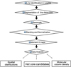 |
Fig. 1 Flowchart of the molecular spectral line stacking and hot core candidate identification. |
3.1.1 Standard spectrum of G9.62+0.19
We first constructed a template for hot core spectral lines using the two broad spectral windows, designated as SPW 7 and SPW 8 in the ATOMS survey, from the well-known source I18032-2032 (G9.62 +0.19). Since G9.62+0.19 contains four confirmed hot cores and displays a line forest of COMs at each core, it serves as a good template for hot cores (Watt et al. 1999; Testi et al. 2000; Liu 2000; Stecklum et al. 2002; Gibb et al. 2004; Linz et al. 2005; Liu et al. 2020b; Peng et al. 2022). Figure B.1 (on Zenodo) presents the full-band spectral lines of three hot cores (C1, C2, and C3) in G9.62+0.19. They exhibit spatially identical peaks of continuum and COM emission. Their peak spectra were extracted using CASA (McMullin et al. 2007; CASA Team 2022) and fit using XCLASS1 (Möller et al. 2017) following Peng et al. (2022), assuming local thermodynamic equilibrium (LTE). The critical density of the relevant transitions is typically 106 cm−3 (Goldsmith 2001). The size of a hot core is very compact, with number densities generally above this threshold; therefore, the LTE assumption is valid (Liu et al. 2021). For CH3OH, CH3OCHO, C2H5OH, CH3OCH3, and CH3CHO, the fit parameters from C1 were adopted as the standard parameters. CH3COCH3 and C2H5OH molecules were not detected in C1 (Peng et al. 2022). We adopted the parameters of CH3COCH3 and C2H5OH from the fits of C2 and C3, respectively. For each species, the XCLASS fitting parameters, including the source size, rotational temperature, column density, line width, and the core from which the spectrum was extracted, are listed in Table A.1.
A noise-free standard spectrum was then modeled using XCLASS, adopting the fit parameters (Table A.1), with the velocity offsets set to zero. The standard spectrum, after stacking (Sect. 3.1.4), was adopted to calibrate the column density of the stacked spectra for the entire sample (Sect. 3.2.3). All the transitions adopted for stacking (Sect. 3.1.2) are optically thin in the standard spectrum, and it is therefore natural to assume the same for other hot cores, especially ones with weak COM emission, which are the focus of our study. We note that, in the optically thin limit, both the column density and spectral intensity will be modified by the same beam dilution factor, and their ratio will remain unchanged.
3.1.2 Transitions and weights for stacking
For each of the seven COM species (Sect. 2), by carefully checking the observed spectra and the standard spectrum, we identified the transitions that are: (1) detected in the hot cores of G9.62+0.19 (see upper panels in Figure 3), and (2) unblended with transitions of any other molecular lines. We note that the CH3OH 2(1)-2(1) transition at a rest frequency of frest = 97582.898 MHz (Table B.1) is not included in the stacking. It has a low Eu of 20 K, which makes its emission typically optically thick and extensively distributed in high-mass star-forming regions. All necessary molecular line information from the Jet Propulsion Laboratory (JPL2) molecular databases (Pickett et al. 1998) are accessed through XCLASS. The rest frequencies of these unblended transitions are listed in Table A.1.
In XCLASS, the conversion between the brightness temperature (in K) and the flux intensity of a line was conducted using the following equation:
![Mathematical equation: $\[T=1.222 \times 10^3 \frac{I}{\nu^2 \theta_{\mathrm{maj}} \theta_{\mathrm{min}}},\]$](/articles/aa/full_html/2025/05/aa52762-24/aa52762-24-eq1.png) (1)
(1)
where I [mJy/beam] denotes the peak flux density, ν [GHz] is the rest frequency of the line (obtained from JPL), and θmaj and θmin [arcsec] represent the major and minor axis lengths of the ALMA synthesized beam at the observed frequency, respectively. The peak brightness temperatures of these transitions on the XCLASS-fit noise-free spectra of G9.62+0.19 are adopted as the weights for line stacking in the following analysis. The weights are also listed in Table A.1.
3.1.3 Resampling
The second and third steps were to cut out and resample the data cube. For each ATOMS source, we cut out a spectral cube with a bandwidth of ~60 km s−1 for each transition selected above. The central frequency of the spectral cube is
![Mathematical equation: $\[\nu_c=\nu_0\left(1-\frac{V_{\mathrm{LSR}}}{c}\right),\]$](/articles/aa/full_html/2025/05/aa52762-24/aa52762-24-eq2.png) (2)
(2)
where VLSR is the systematic velocity of the source, ν0 is the rest frequency of the transition, and c represents the speed of light. Next, we converted the frequency axis (ν) into the velocity axis (V) using the relation
![Mathematical equation: $\[V=\frac{\nu_c-\nu}{\nu_c} c.\]$](/articles/aa/full_html/2025/05/aa52762-24/aa52762-24-eq3.png) (3)
(3)
It should be noted that, for a given species, the velocity resolutions of its different transitions may vary. To align the velocity channels, we further resampled the cut cube of each transition to a velocity resolution of 1.25 km s−1.
3.1.4 Spectral stacking and normalization
In the fourth step outlined in Figure 1, the stacked cube ![Mathematical equation: $\[\left(D_{j}^{i}\right)\]$](/articles/aa/full_html/2025/05/aa52762-24/aa52762-24-eq4.png) for each species (j) of each source (i) was obtained by averaging the resampled cubes (
for each species (j) of each source (i) was obtained by averaging the resampled cubes (![Mathematical equation: $\[D_{j ; k}^{i}\]$](/articles/aa/full_html/2025/05/aa52762-24/aa52762-24-eq5.png) ) of different transitions (denoted as k; see Sect. 3.1.2), weighted according to the values (denoted as Wk) in Table A.1, as is shown below
) of different transitions (denoted as k; see Sect. 3.1.2), weighted according to the values (denoted as Wk) in Table A.1, as is shown below
![Mathematical equation: $\[D_j^i=\frac{\sum ~W_k D_{j ; k}^i}{\sum ~W_k}.\]$](/articles/aa/full_html/2025/05/aa52762-24/aa52762-24-eq6.png) (4)
(4)
If the intensities of the different transitions of the same species are proportional to those of the template spectra (Sect. 3.1.2) and exhibit the same noise level, this set of weights could achieve the highest S/N for the stacked cube (Liu et al. 2022). The stacked spectra of the seven COM species, obtained by applying the above procedure to the standard spectrum of G9.62+0.19 (Sect. 3.1.1), are presented in Fig. 2.
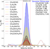 |
Fig. 2 The stacked model spectrum of the seven molecules. The solid lines represent the averaged spectra of the template hot cores in G9.62 +0.19 after spectral stacking. The dashed lines show Gaussian fits to the spectra. The integrated areas of the Gaussian fits (in units of Kelvin kilometers per second) are labeled in the upper right corner. The vertical dotted lines indicate the velocity range of ±5 km/s. |
3.1.5 Integrated intensity maps of stacked cubes
After stacking, we integrated the emission for the stacked lines within a velocity range of ± 5 km s−1. We chose this value because the typical COM line width, measured as the full width at half maximum (FWHM), for the strong sample of hot cores is approximately 5 km s−1 (Liu et al. 2020b). As is shown in Figure 2, the adopted velocity range for integration covers the majority of the emission in the stacked spectra of G9.62+0.19, while avoiding blending.
Figure 3 shows the integrated intensity maps (moment 0 maps) of the stacked cubes of the seven species for I18032-2032, I15394-5358, and I18434-0242. I18032-2032 (G9.62+0.19) contains four hot cores, labeled as C1, C2, C3, and C4, which were previously identified by Peng et al. (2022) and Qin et al. (2022). This source has the largest number of hot cores in the sample. Its gas kinetic temperature and column density serve as a reference for typical hot cores. I15394-5358 and I18434-0242 are examples of sources with newly identified hot core candidates in this work. The moment 0 maps of the seven species for the other sources that exhibit at least one compact core of CH3OH are displayed in Figure C.1 (on Zenodo).
3.2 Hot core candidates
3.2.1 Identification
We identified hot molecular core (HMC) candidates from the moment 0 maps of the stacked cubes. An HMC candidate was visually identified by the presence of strong (≳5σ), compact CH3OH emission. Here, a compact core is defined as one with a round morphology, where its central brightest part is not resolved or is only partly resolved under the current spatial resolution (Sect. 2). In total, we identified 100 HMC candidates, 60 of which are identical to the ones in the strong sample previously identified by Qin et al. (2022), and the remaining 40 of which are weak candidates newly identified in this work.
These HMC candidates are typically associated with compact emission in other COMs as well. Figure 4 shows the statistics of line detection for all 100 HMC candidates. All 40 newly identified HMC candidates exhibit compact emission of CH3OCHO or C2H5CN. Specifically, 36 show CH3OCHO emission, 29 display C2H5CN emission, 5 reveal C2H5OH emission, 25 demonstrate CH3OCH3 emission, 16 present CH3CHO emission, and only one core shows CH3COCH3 emission. All 60 hot cores previously identified by Qin et al. (2022) exhibit stronger CH3OH emission and more individual COM line transitions than the newly identified weak hot core candidates. In total, 100 hot cores show CH3OH emission, 90 show CH3OCHO emission, 80 show C2H5CN emission, 46 show C2H5OH emission, 77 show CH3OCH3 emission, 59 show CH3CHO emission, and 27 show CH3COCH3 emission.
3.2.2 Two-dimensional Gaussian fitting
Two-dimensional Gaussian fitting was applied to the 100 cores on the moment 0 maps of CH3OH using the CASA imfit procedure. The beam-deconvolved fitting parameters were adopted, including the source size (θsource), the position angle (PA), the peak flux of the integrated intensity (Ipeak; in units of K km s−1), and the total flux of the integrated intensity (Iintegrated; in units of Kelvin kilometers per second per square arcsecond). Here, ![Mathematical equation: $\[\theta_{\text {source }}=\sqrt{a b}\]$](/articles/aa/full_html/2025/05/aa52762-24/aa52762-24-eq7.png) , where a and b represent the deconvolved major and minor FWHM axes of the cores. The sizes of molecular CH3OH emission range from 1092 to 46 884 AU for sources at different distances. The fit peak positions, θsource, PA, Ipeak, and Iintegrated, of CH3OH are summarized in Table B.2.
, where a and b represent the deconvolved major and minor FWHM axes of the cores. The sizes of molecular CH3OH emission range from 1092 to 46 884 AU for sources at different distances. The fit peak positions, θsource, PA, Ipeak, and Iintegrated, of CH3OH are summarized in Table B.2.
The same fitting procedure was applied for the other six COM species (if detected). For some hot cores, the emission of CH3CHO displays extended components, making the fitting of CH3CHO less reliable. The extended emission of CH3CHO is discussed further in Sect. 4.3. The fit parameters of the six species are summarized in Tables B.3 and B.4.
3.2.3 Column density
G9.62+0.19 was adopted as the calibration source to estimate the column densities of hot core candidates from their stacked emission. For each species, we integrated the standard spectrum of G9.62+0.19 (after stacking for each species; see Sects. 3.1.1 and 3.1.4) within a velocity range of ± 5 km s−1 (Fig. 2) to obtain the standard integrated intensity (Icali) of the stacked spectrum for that species. This allowed us to quickly determine the intensity of each species by focusing on the relevant spectral features. The column density of the G9.62+0.19 hot-core value, provided in Sect. 3.1.1 and listed in Table A.1, was adopted as the standard column density (denoted as Ncali) for the corresponding species. To evaluate the column density of each species, we used the following conversion formula:
![Mathematical equation: $\[N=\frac{N_{\mathrm{cali}}}{I_{\mathrm{cali}}} I.\]$](/articles/aa/full_html/2025/05/aa52762-24/aa52762-24-eq8.png) (5)
(5)
Here, I represents the integrated intensity of the stacked spectrum, and this formula allowed us to scale the species’ column density relative to the standard value.
Applying Eq. (5) to the moment 0 map of a stacked cube results in a column density map for the corresponding species. In Sect. 3.1.5, we have already obtained the beam-deconvolved peak value (Ipeak) of the moment map using 2D Gaussian fitting, enabling us to directly calculate the beam-deconvolved peak column density using Eq. (5). The derived column densities of different species are listed in Tables B.2, B.3, and B.4.
In Figure 5, we compare the beam-deconvolved column densities (Sect. 3.2.3) calculated using the spectral stacking method with the ones derived by Qin et al. (2022) through LTE fitting for the 60 strong hot cores. The results are generally in good agreement, supporting the reliability of column densities estimated through stacking. The details of the hot cores in G9.62+0.19 remain unclear, and we cannot confirm whether different hot core candidates exhibit similar distributions of emitting regions and excitation conditions. The discrepancy in the column densities primarily arises from possible differences in excitation temperatures and spatial patterns of COM emission in G9.62+0.19. Although the transitions chosen for stacking are optically thin, unresolved optically thick regions that cannot be distinguished at the current resolution may also contribute to the discrepancy. Nonetheless, the good agreement between the XCLASS fitting and the stacking conversion suggests comparable excitation conditions for different hot core candidates.
The column densities of the seven molecules span a striking range, covering one to three orders of magnitude. CH3OH stands out with the highest column densities, ranging from 1.4 × 10¹⁸ to 4.4 × 1020 cm−2. In comparison, CH3OCHO and CH3OCH3 show column densities approximately half an order of magnitude lower, from 5.3 × 10¹⁷ to 2.8 × 1020 cm−2 and from 1.0 × 10¹⁸ to 1.4 × 1020 cm−2, respectively. C2H5OH, CH3CHO, and CH3COCH3 exhibit column densities roughly one order of magnitude lower than CH3OH, ranging from 1.3 × 10¹⁷ to 5.9 × 1019 cm−2. C2H5CN, with the lowest values, spans a range from 1.6 × 10¹⁵ to 7.1 × 1018 cm−2-roughly two orders of magnitude lower than CH3OH. This wide variability in column densities highlights the diverse physical conditions or evolution stages among the 100 hot core candidates under investigation.
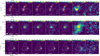 |
Fig. 3 Moment 0 maps of the stacked cubes (Sect. 3.1.5) from three example sources – I18032-2032 (G9.62+0.19), I15394-5358, and I18434-0242 – are shown. The contours represent the continuum emission, with levels of [5, 10, 30, 50, 100, 200] multiplied by the root mean square (rms). The rms value is shown in the lower right corner of the figure (in units of Jansky per beam. The white filled white ellipses in the lower right corners of the left panels represent the beam of continuum emission. The red ellipses indicate the deconvolved FWHM sizes from the twodimensional Gaussian fits to the compact cores. The images for the remaining 83 sources, which contain 94 hot cores and candidates, are presented in Fig. C.1 (on Zenodo). |
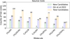 |
Fig. 4 Number of hot cores detected with different COMs. The numbers from Qin et al. (2022), the newly detected numbers from this work, and the total are presented. |
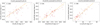 |
Fig. 5 Comparison of column densities derived through stacking (y axis; Sect. 3.2.3) and those fit by Qin et al. (2022) (x axis) for the 60 brightest hot cores. The yellow line represents y = x. C denotes the correlation coefficient. |
4 Discussion
4.1 Source-stacking spectrum of hot-cores
For each of the 100 hot core candidates, we extracted the fullband spectra of SPW 7 and SPW 8 at the peak location of CH3OH (after stacking). First, these frequency axis of these spectra were corrected through
![Mathematical equation: $\[v^{\prime}=\left(1+\frac{V_{\mathrm{LSR}}}{c}\right) v.\]$](/articles/aa/full_html/2025/05/aa52762-24/aa52762-24-eq9.png) (6)
(6)
Here, v′ is the corrected frequency axis. We then resampled the spectra to have aligned channels with a channel width of 0.49 MHz. A source-stacking template spectrum was obtained by averaging these spectra with equal weighting. The stacked spectrum is shown in Figure 6. Thanks to the improved S/N from source stacking, the rich emission lines of COMs can be identified. We fit the template spectrum with the emissions of species already identified from G9.62+0.19 (Liu et al. 2020b; Peng et al. 2022) using XCLASS. The rest frequencies, transitions, and state temperatures of these molecules are compiled in Table B.1. The source-stacking spectrum can serve as a template for HMC studies, providing a reference for the rapid identification of molecular species in the same band. In addition to the identified transitions, there are plenty of line features yet to be identified in the ATOMS sample. We do not attempt to identify them in this work, which focuses on spectral stacking of the ATOMS hot core candidates. Instead, the source-stacking spectrum offers a valuable template for hot-core research in future studies. The source-stacking technique can also enhance sensitivity for molecular identification in follow-up surveys, such as the ALMA-QUARKS survey in band 6 (Liu et al. 2024b).
4.2 Correlations of complex molecules
Figures 7 and C.2 (on Zenodo) show the correlations between the column densities of molecular pairs for the seven molecules, including both the strong hot cores and the weak candidates. One of the most significant features is that the column densities of weak hot core candidates lie at the lower end of the linear correlation trend for different COM species across the entire sample. This supports the validity of estimating column density through stacking (Sect. 3.2.3) and may suggest that the similarity in excitation conditions observed in hot cores could also be applicable to the weak hot core candidates.
We summarized the correlation coefficients of different molecular pairs in the lower-right panel of Figures 7. Among them, three molecular pairs exhibited strong correlations (with correlation coefficients close ≳ 0.9): CH3OH versus CH3OCHO, CH3OCHO versus C2H5CN, and CH3OCHO versus CH3OCH3 (Figure 7). Their correlation coefficients are 0.89, 0.88, and 0.94, respectively. CH3OH, CH3OCHO, and C2H5CN demonstrate consistently strong correlations in their column densities.
The strong correlation between CH3OCHO and CH3OCH3 has been observed in low-(Li et al. 2024), intermediate-(Ospina-Zamudio et al. 2018), and high-mass star-forming regions (e.g., Bisschop et al. 2007; Coletta et al. 2020; Li et al. 2024). This close relationship can be attributed to a common precursor, CH3O (Garrod & Herbst 2006; Garrod et al. 2008; Garrod 2013; Öberg 2016), or alternatively CH3OCH3 may act as a precursor to CH3OCHO (Balucani et al. 2015). Moreover, both species are strongly correlated with CH3OH (Fig. 7), supporting the hypothesis that their precursor, CH3O, is likely produced through the photodissociation of CH3OH in a hot-core environment. As an isomer of CH3OCH3, C2H5OH also exhibits a strong correlation (0.86) with CH3OCHO. This suggests that the chemical environments for forming the two isomers (C2H5OH and CH3OCH3) in hot cores share similarities.
The weakest correlation occurs between CH3OH and CH3COCH3. This can be attributed to the distinct formation and excitation mechanisms of these molecules. CH3OH is abundant in hot cores and may form primarily through grain-surface reactions (Herbst & van Dishoeck 2009). In contrast, CH3COCH3 (acetone) is a more complex molecule that forms through both gas-phase reactions and surface reactions on dust grains (Combes et al. 1987; Singh et al. 2022). The differences in their formation pathways could lead to varying physical conditions in hot cores, which may result in the observed weak correlation.
The strong correlation between the nitrogen-bearing molecule C2H5CN and the oxygen-bearing molecule CH3OCHO confirms that both are excellent tracers of hot cores, with the hot core environment governing their generation and/or the excitation of their emission. C2H5CN also shows a strong overall correlation with CH3OCH3, with a correlation coefficient of 0.86. However, different spatial distributions between the nitrogen-bearing C2H5CN and oxygen-bearing species are observed in some sources (e.g., IRAS 17158-3901, 17160-3707, and 18032-2032; see Figure C.3 (on Zenodo)). Therefore, whether the nitrogen and oxygen differentiation is common in our sample of high-mass star-forming regions remains uncertain due to the limited angular resolution in our observations (Qin et al. 2022). In future studies utilizing higher-resolution and more sensitive data from the ALMA-QUARKS project (Liu et al. 2024b), a more comprehensive analysis of the differentiation between nitrogen and oxygen species in hot cores will be achievable.
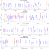 |
Fig. 6 Spectrum averaged over all 100 hot core candidates (Sect. 4.1). The transitions identified in the averaged spectrum (see Table B.1) are labeled with the corresponding species names. The transitions selected for spectral stacking (Sect. 3.1.2) in this work are marked with red labels displaying the species names. The 3σ (0.2 K) noise level is indicated by horizontal pink lines. |
4.3 Spatial distributions of complex molecular line emission
The emission lines of COMs, with the exception of CH3CHO, generally exhibit compact emission, concentrated around the average position of the peak emission of the seven molecules. In contrast, CH3CHO displays more extended emission in certain sources, such as I8032-2032 and I15394-5358, as is shown in Figure 3. The sizes of the emission regions for the seven molecules were measured in each source and are compared in Figure 8. The deconvolved sizes of the emission regions for CH3OH, CH3OCHO, C2H5CN, C2H5OH, CH3OCH3, and CH3COCH3 range from approximately 940 to 57 306 AU, while the deconvolved sizes for CH3CHO range from 4033 to 91 884 AU.
We compared the integrated intensity maps of the stacked cube of CH3CHO with the ones of SiO (2–1) and H13CO+ (1–0), both of which typically exhibit extended emission in the ATOMS sample. In 43 sources, CH3CHO shows emission that is as extended as that of SiO and H13CO+, as is demonstrated in Figure 9. To quantify this, we calculated the correlation between the integrated intensity maps of CH3CHO, SiO, and H13CO+for these 43 sources. The distribution of the correlation coefficients is shown in Figure 10. We find that CH3CHO exhibits a strong correlation with H13CO+, with correlation coefficients exceeding 0.8. This suggests that CH3CHO is likely widely distributed throughout some high-mass star-forming regions, similar to H13CO+, a common tracer of dense gas. In particular, for several sources (I13079-6218, I13134-6242, I13140-6226, I16071-5142, I16272-4837, I16318-4724, I16348-4654, and I18507+0121), CH3CHO shows a strong correlation with SiO, with correlation coefficients greater than 0.8. This finding supports the possibility that CH3CHO could be formed in shock-processed regions, a hypothesis that warrants further investigation in future studies (Chengalur & Kanekar 2003).
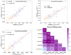 |
Fig. 7 Comparison of the column density correlations among the seven molecules. The first three panels show the correlations of molecular column densities, with the red lines representing the linear fit in log scale. The correlation coefficients (labeled as ‘C’ in the upper left corner) are displayed in each panel. Blue and yellow points represent the column densities obtained through stacking of the 60 strong hot cores and 40 weak candidates, respectively. Gray points indicate the column densities of strong hot cores fit by Qin et al. (2022). The bottom right panel displays the correlation coefficients between all species. Each cell is colored, with a deeper color representing a higher correlation coefficient. The p value, which is also displayed in each panel, quantifies the statistical significance of the observed correlation. A smaller p value (typically <0.05) indicates a stronger, more statistically significant correlation, while larger p value suggest weaker or less significant relationships between the variables. |
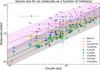 |
Fig. 8 Relation between the beam-deconvolved sizes (in log scale) of hot core candidates for different species, with the x and y axes values representing the core sizes of CH3OH and the other six species, respectively. The dashed red line represents y = x. The dashed black line shows the linear fit of all data points, except those of CH3CHO. The dashed pink line shows the linear fit of the CH3CHO data. The shaded regions indicate the standard deviation range of the data. |
5 Conclusions
We conducted a systematic survey of hot molecular cores in 146 high-mass star forming regions using the ATOMS band 3 data through molecular spectral stacking technique. The complex molecules used in this study are CH3OH, CH3OCHO, C2H5CN, C2H5OH, CH3OCH3, CH3CHO, and CH3COCH3. The primary findings of this work are summarized as follows:
- (1)
Using spectral stacking techniques, we identified 100 hot core candidates that show strong and compact COMs emissions. Among them, 60 hot cores were previously identified by Qin et al. (2022). The other 40 are newly identified in this work.
- (2)
We estimated the column densities for seven molecules at the peak positions of the CH3OH emission. Among the seven molecules, CH3OH has the highest column density. The column densities of CH3OCHO and CH3OCH3 are approximately half an order of magnitude lower than that of CH3OH. C2H5OH, CH3CHO, and CH3COCH3 are an order of magnitude lower, while C2H5CN is about two orders of magnitude lower than CH3OH.
(3) A tight correlation between the column densities of CH3OCHO and CH3OCH3 (correlation coefficient of 0.94) is found in our hot core sample. Strong correlations are also witnessed between the pairs of CH3OCHO/CH3OH, CH3OCH3/CH3OH, and C2H5OH/CH3OCHO. These chemical links suggest that CH3OH serves as a precursor for several COMs.
(4) CH3CHO exhibits significantly extended emission in 43 of the 100 hot core candidates. The extended emission features of CH3CHO in these 43 sources are similar to the ones of SiO and H13CO+. This suggests that CH3CHO is widely distributed and may be formed in shock regions within some high-mass star-forming clumps.
Overall, this study significantly expands the sample of hot core candidates through the spectral stacking method, providing a reliable approach for identifying molecular species in high-=mass star-forming regions. The method serves as a valuable tool for future investigations into molecular distributions and formation processes in these environments.
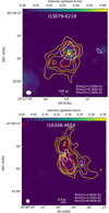 |
Fig. 9 Comparison of moment 0 maps of CH3CHO (after spectral stacking), SiO, and H13CO+. The background emission shows 3 mm continuum emission. The white, yellow and red contours are for H13CO+ emission, SiO, and CH3CHO, respectively. Their contour levels are [5, 10, 15, 30, 50, 100, 200] × Rms(1, 2, 3). Rms(1), Rms(2) and Rms(3) are shown in the lower right corners, representing the noise values for CH3CHO, SiO, and H13CO+, respectively, with units of Kelvin kilometers per second. The beam of continuum emission is placed in the lower left corner of the image. |
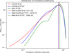 |
Fig. 10 Kernel density estimate (KDE) smoothed distribution of correlation coefficients between the moment 0 maps of CH3CHO (after stacking), SiO (2–1), and H13CO+ (1–0). The KDE curves were generated using the gaussian_kde tool from the scipy package in Python. The vertical lines indicate the peaks of the distributions. |
Data availability
The derived data underlying this article are available in thearticle and in its online supplementary material on Zenodo.
Full Tables B.1–B.4 are available at the CDS via anonymous ftp to cdsarc.cds.unistra.fr (130.79.128.5) or via https://cdsarc.cds.unistra.fr/viz-bin/cat/J/A+A/697/A190
Acknowledgements
This work has been supported by the National Key R&D Program of China (No. 2022YFA1603100). X.L. acknowledges the support of the Strategic Priority Research Program of the Chinese Academy of Sciences under Grant No. XDB0800303. T.L. acknowledges support from the National Natural Science Foundation of China (NSFC), through grants No. 12073061 and No. 12122307, the Tianchi Talent Program of Xinjiang Uygur Autonomous Region. S.-L. Qin is supported by National Natural Science Foundation of China (NSFC) through grant No.12033005. This research was carried out in part at the Jet Propulsion Laboratory, California Institute of Technology, under a contract with the National Aeronautics and Space Administration (80NM0018D0004). Y.P. Peng acknowledges support from NSFC through grant No. 12303028. L.B. and G.G. acknowledge support by the ANID BASAL project FB210003. C.W.L. acknowledges support from the Basic Science Research Program through the NRF funded by the Ministry of Education, Science and Technology (NRF-2019R1A2C1010851) and from the Korea Astronomy and Space Science Institute grant funded by the Korea government (MSIT; project No. 2024-1-841-00). PS was partially supported by a Grant-in-Aid for Scientific Research (KAKENHI Number JP22H01271 and JP23H01221) of JSPS. H.-L. Liu is supported by Yunnan Fundamental Research Project (grant No. 202301AT070118, 202401AS070121), and by Xingdian Talent Support Plan–Youth Project.
Appendix A Parameters of molecular transitions
Parameters of molecular transitions
Appendix B Additional tables
Table B.1 shows the molecular line parameters for lines marked in Figure 6. Table B.2 lists line parameters of CH3OH. Table B.3-B.4 lists the Physical parameters of CH3OCHO C2H5CN C2H5OH CH3OCH3 CH3CHO CH3COCH3.
Identified transitions from stacked spectra of 100 hot cores
Line parameters of CH3OH
Appendix C Additional figures
Figure C.1 (on Zenodo) shows the spectral lines of three cores (C1, C2, C3) in G9.62 +0.19, with the molecular spectral lines in Table A.1 annotated. Figure C.2 (on Zenodo) presents the correlations of molecular column densities. Figure C.3 (on Zenodo) illustrates the comparison of moment 0 maps of CH3CHO (after spectral stacking), SiO and H13CO+.
Appendix D Moment maps
Figure D.1 (on Zenodo) displays the moment 0 map obtained by stacking seven molecules.
Physical parameters of CH3OCHO C2H5CN C2H5OH
Physical parameters of CH3OCH3 CH3CHO CH3COCH3
References
- Agúndez, M., Loison, J. C., Hickson, K. M., et al. 2023, A&A, 673, A34 [NASA ADS] [CrossRef] [EDP Sciences] [Google Scholar]
- Balucani, N., Ceccarelli, C., & Taquet, V. 2015, MNRAS, 449, L16 [Google Scholar]
- Beuther, H., Mottram, J. C., Ahmadi, A., et al. 2018, A&A, 617, A100 [NASA ADS] [CrossRef] [EDP Sciences] [Google Scholar]
- Bigiel, F., Leroy, A. K., Jiménez-Donaire, M. J., et al. 2016, ApJ, 822, L26 [NASA ADS] [CrossRef] [Google Scholar]
- Bisschop, S. E., Jørgensen, A. A., van der Wal, L. H., de Jong, C. W. M., & Herbst, E. 2006, A&A, 445, 907 [Google Scholar]
- Bisschop, S. E., Jørgensen, J. K., van Dishoeck, E. F., & de Wachter, E. B. M. 2007, A&A, 465, 913 [NASA ADS] [CrossRef] [EDP Sciences] [Google Scholar]
- Bonfand, M., Csengeri, T., Bontemps, S., et al. 2024, A&A, 687, A163 [NASA ADS] [CrossRef] [EDP Sciences] [Google Scholar]
- Caldú-Primo, A., Schruba, A., Walter, F., et al. 2013, AJ, 146, 150 [CrossRef] [Google Scholar]
- CASA Team (Bean, B., et al.) 2022, PASP, 134, 114501 [NASA ADS] [CrossRef] [Google Scholar]
- Cesaroni, R. 2005, in Massive Star Birth: A Crossroads of Astrophysics, eds. R. Cesaroni, M. Felli, E. Churchwell, & M. Walmsley, IAU Symposium, 227, 59 [Google Scholar]
- Chen, Y., van Gelder, M. L., Nazari, P., et al. 2023, A&A, 678, A137 [NASA ADS] [CrossRef] [EDP Sciences] [Google Scholar]
- Chengalur, J. N., & Kanekar, N. 2003, MNRAS, 341, 1639 [Google Scholar]
- Coletta, A., Fontani, F., Rivilla, V. M., et al. 2020, A&A, 641, A54 [NASA ADS] [CrossRef] [EDP Sciences] [Google Scholar]
- Combes, F., Gerin, M., Wootten, A., et al. 1987, A&A, 180, L13 [Google Scholar]
- Delhaize, J., Meyer, M. J., Staveley-Smith, L., & Boyle, B. J. 2013, MNRAS, 433, 1398 [NASA ADS] [CrossRef] [Google Scholar]
- Dib, S., Shadmehri, M., Padoan, P., et al. 2010, MNRAS, 405, 401 [NASA ADS] [Google Scholar]
- Fontani, F., Pascucci, I., Caselli, P., et al. 2007, A&A, 470, 639 [NASA ADS] [CrossRef] [EDP Sciences] [Google Scholar]
- Garrod, R. T. 2013, ApJ, 765, 60 [Google Scholar]
- Garrod, R. T., & Herbst, E. 2006, A&A, 457, 927 [NASA ADS] [CrossRef] [EDP Sciences] [Google Scholar]
- Garrod, R. T., Widicus Weaver, S. L., & Herbst, E. 2008, ApJ, 682, 283 [Google Scholar]
- Gibb, A. G., Wyrowski, F., & Mundy, L. G. 2004, ApJ, 616, 301 [Google Scholar]
- Gibb, E., Nummelin, A., Irvine, W. M., Whittet, D. C. B., & Bergman, P. 2000, ApJ, 545, 309 [NASA ADS] [CrossRef] [Google Scholar]
- Ginsburg, A., McGuire, B. A., Sanhueza, P., et al. 2023, ApJ, 942, 66 [Google Scholar]
- Goldsmith, P. F. 2001, ApJ, 557, 736 [Google Scholar]
- Herbst, E., & van Dishoeck, E. F. 2009, ARA&A, 47, 427 [NASA ADS] [CrossRef] [Google Scholar]
- Hernández-Hernández, V., Zapata, L., Kurtz, S., & Garay, G. 2014, ApJ, 786, 38 [Google Scholar]
- Jørgensen, J. K., van der Wiel, M. H. D., Coutens, A., et al. 2016, A&A, 595, A117 [Google Scholar]
- Jørgensen, J. K., Belloche, A., & Garrod, R. T. 2020, ARA&A, 58, 727 [Google Scholar]
- Karim, A., Schinnerer, E., Martínez-Sansigre, A., et al. 2011, ApJ, 730, 61 [Google Scholar]
- Knudsen, K. K., van der Werf, P., Franx, M., et al. 2005, ApJ, 632, L9 [NASA ADS] [CrossRef] [Google Scholar]
- Kurtz, S., Cesaroni, R., Churchwell, E., Hofner, P., & Walmsley, C. M. 2000, in Protostars and Planets IV, eds. V. Mannings, A. P. Boss, & S. S. Russell, 299 [Google Scholar]
- Li, C., Qin, S.-L., Liu, T., et al. 2024, MNRAS, 533, 1583 [NASA ADS] [CrossRef] [Google Scholar]
- Lindroos, L., Knudsen, K. K., Fan, L., et al. 2016, MNRAS, 462, 1192 [NASA ADS] [CrossRef] [Google Scholar]
- Linz, H., Stecklum, B., Henning, T., Hofner, P., & Brandl, B. 2005, A&A, 429, 903 [NASA ADS] [CrossRef] [EDP Sciences] [Google Scholar]
- Liu, S. Y. 2000, in American Astronomical Society Meeting Abstracts, 197, 132.01 [Google Scholar]
- Liu, T., Evans, N. J., Kim, K.-T., et al. 2020a, MNRAS, 496, 2821 [Google Scholar]
- Liu, T., Evans, N. J., Kim, K.-T., et al. 2020b, MNRAS, 496, 2790 [Google Scholar]
- Liu, H.-L., Liu, T., Evans, Neal J., I., et al. 2021, MNRAS, 505, 2801 [NASA ADS] [CrossRef] [Google Scholar]
- Liu, X., Liu, T., Shen, Z., et al. 2022, ApJS, 263, 13 [NASA ADS] [CrossRef] [Google Scholar]
- Liu, X., Liu, T., Shen, Z., et al. 2023, A&A, 671, L1 [NASA ADS] [CrossRef] [EDP Sciences] [Google Scholar]
- Liu, X., Liu, T., Shen, Z., et al. 2024a, ApJS, 271, 3 [NASA ADS] [CrossRef] [Google Scholar]
- Liu, X., Liu, T., Zhu, L., et al. 2024b, Res. Astron. Astrophys., 24, 025009 [CrossRef] [Google Scholar]
- McGuire, B. A. 2022, ApJS, 259, 30 [NASA ADS] [CrossRef] [Google Scholar]
- McGuire, B. A., Pearson, J. C., Williams, T. D., & McCall, D. M. W. P. K. H. J. 2016, ApJ, 819, 47 [CrossRef] [Google Scholar]
- McMullin, J. P., Waters, B., Schiebel, D., Young, W., & Golap, K. 2007, in Astronomical Data Analysis Software and Systems XVI, eds. R. A. Shaw, F. Hill, & D. J. Bell, Astronomical Society of the Pacific Conference Series, 376, 127 [NASA ADS] [Google Scholar]
- Möller, T., Endres, C., & Schilke, P. 2017, A&A, 598, A7 [NASA ADS] [CrossRef] [EDP Sciences] [Google Scholar]
- Neumann, L., den Brok, J. S., Bigiel, F., et al. 2023, A&A, 675, A104 [NASA ADS] [CrossRef] [EDP Sciences] [Google Scholar]
- Öberg, K. I. 2016, Chem. Rev., 116, 9631 [Google Scholar]
- Offner, S. S. R., Moe, M., Kratter, K. M., et al. 2023, in Protostars and Planets VII, eds. S. Inutsuka, Y. Aikawa, T. Muto, K. Tomida, & M. Tamura, Astronomical Society of the Pacific Conference Series, 534, 275 [NASA ADS] [Google Scholar]
- Ospina-Zamudio, J., Lefloch, B., Ceccarelli, C., et al. 2018, A&A, 618, A145 [NASA ADS] [CrossRef] [EDP Sciences] [Google Scholar]
- Pabst, C. H. M., Goicoechea, J. R., Cuadrado, S., et al. 2024, A&A, 688, A7 [NASA ADS] [CrossRef] [EDP Sciences] [Google Scholar]
- Peng, Y., Liu, T., Qin, S.-L., et al. 2022, MNRAS, 512, 4419 [CrossRef] [Google Scholar]
- Pickett, H. M., Poynter, R. L., Cohen, E. A., et al. 1998, J. Quant. Spec. Radiat. Transf., 60, 883 [Google Scholar]
- Qin, S.-L., Liu, T., Liu, X., et al. 2022, MNRAS, 511, 3463 [CrossRef] [Google Scholar]
- Schilke, P., Groesbeck, T. D., Blake, G. A., Phillips, & T. G. 1997, ApJS, 108, 301 [NASA ADS] [CrossRef] [Google Scholar]
- Schilke, P., Benford, D. J., Hunter, T. R., Lis, D. C., & Phillips, T. G. 2001, ApJS, 132, 281 [Google Scholar]
- Schilke, P., Comito, C., Thorwirth, S., et al. 2006, A&A, 454, L41 [NASA ADS] [CrossRef] [EDP Sciences] [Google Scholar]
- Schruba, A., Leroy, A. K., Walter, F., et al. 2011, AJ, 142, 37 [NASA ADS] [CrossRef] [Google Scholar]
- Singh, S. K., Fabian Kleimeier, N., Eckhardt, A. K., & Kaiser, R. I. 2022, ApJ, 941, 103 [Google Scholar]
- Stecklum, B., Brandl, B., Feldt, M., et al. 2002, in The Origin of Stars and Planets: The VLT View, eds. J. F. Alves. & M. J. McCaughrean, 225 [Google Scholar]
- Taniguchi, K., Sanhueza, P., Olguin, F. A., et al. 2023, ApJ, 950, 57 [CrossRef] [Google Scholar]
- Testi, L., Hofner, P., Kurtz, S., & Rupen, M. 2000, A&A, 359, L5 [NASA ADS] [Google Scholar]
- Tychoniec, Ł., van Dishoeck, E. F., van’t Hoff, M. L. R., et al. 2021, A&A, 655, A65 [NASA ADS] [CrossRef] [EDP Sciences] [Google Scholar]
- van Dishoeck, E. F., & Blake, G. A. 1998, ARA&A, 36, 317 [Google Scholar]
- Watt, S., Mundy, L. G., & Wyrowski, F. 1999, in American Astronomical Society Meeting Abstracts, 195, 73.07 [Google Scholar]
- Zhou, J. W., Kroupa, P., & Dib, S. 2024, PASP, 136, 094301 [NASA ADS] [CrossRef] [Google Scholar]
- Zinnecker, H., & Yorke, H. W. 2007, ARA&A, 45, 481 [Google Scholar]
All Tables
All Figures
|
Fig. 1 Flowchart of the molecular spectral line stacking and hot core candidate identification. |
| In the text | |
|
Fig. 2 The stacked model spectrum of the seven molecules. The solid lines represent the averaged spectra of the template hot cores in G9.62 +0.19 after spectral stacking. The dashed lines show Gaussian fits to the spectra. The integrated areas of the Gaussian fits (in units of Kelvin kilometers per second) are labeled in the upper right corner. The vertical dotted lines indicate the velocity range of ±5 km/s. |
| In the text | |
|
Fig. 3 Moment 0 maps of the stacked cubes (Sect. 3.1.5) from three example sources – I18032-2032 (G9.62+0.19), I15394-5358, and I18434-0242 – are shown. The contours represent the continuum emission, with levels of [5, 10, 30, 50, 100, 200] multiplied by the root mean square (rms). The rms value is shown in the lower right corner of the figure (in units of Jansky per beam. The white filled white ellipses in the lower right corners of the left panels represent the beam of continuum emission. The red ellipses indicate the deconvolved FWHM sizes from the twodimensional Gaussian fits to the compact cores. The images for the remaining 83 sources, which contain 94 hot cores and candidates, are presented in Fig. C.1 (on Zenodo). |
| In the text | |
|
Fig. 4 Number of hot cores detected with different COMs. The numbers from Qin et al. (2022), the newly detected numbers from this work, and the total are presented. |
| In the text | |
|
Fig. 5 Comparison of column densities derived through stacking (y axis; Sect. 3.2.3) and those fit by Qin et al. (2022) (x axis) for the 60 brightest hot cores. The yellow line represents y = x. C denotes the correlation coefficient. |
| In the text | |
|
Fig. 6 Spectrum averaged over all 100 hot core candidates (Sect. 4.1). The transitions identified in the averaged spectrum (see Table B.1) are labeled with the corresponding species names. The transitions selected for spectral stacking (Sect. 3.1.2) in this work are marked with red labels displaying the species names. The 3σ (0.2 K) noise level is indicated by horizontal pink lines. |
| In the text | |
|
Fig. 7 Comparison of the column density correlations among the seven molecules. The first three panels show the correlations of molecular column densities, with the red lines representing the linear fit in log scale. The correlation coefficients (labeled as ‘C’ in the upper left corner) are displayed in each panel. Blue and yellow points represent the column densities obtained through stacking of the 60 strong hot cores and 40 weak candidates, respectively. Gray points indicate the column densities of strong hot cores fit by Qin et al. (2022). The bottom right panel displays the correlation coefficients between all species. Each cell is colored, with a deeper color representing a higher correlation coefficient. The p value, which is also displayed in each panel, quantifies the statistical significance of the observed correlation. A smaller p value (typically <0.05) indicates a stronger, more statistically significant correlation, while larger p value suggest weaker or less significant relationships between the variables. |
| In the text | |
|
Fig. 8 Relation between the beam-deconvolved sizes (in log scale) of hot core candidates for different species, with the x and y axes values representing the core sizes of CH3OH and the other six species, respectively. The dashed red line represents y = x. The dashed black line shows the linear fit of all data points, except those of CH3CHO. The dashed pink line shows the linear fit of the CH3CHO data. The shaded regions indicate the standard deviation range of the data. |
| In the text | |
|
Fig. 9 Comparison of moment 0 maps of CH3CHO (after spectral stacking), SiO, and H13CO+. The background emission shows 3 mm continuum emission. The white, yellow and red contours are for H13CO+ emission, SiO, and CH3CHO, respectively. Their contour levels are [5, 10, 15, 30, 50, 100, 200] × Rms(1, 2, 3). Rms(1), Rms(2) and Rms(3) are shown in the lower right corners, representing the noise values for CH3CHO, SiO, and H13CO+, respectively, with units of Kelvin kilometers per second. The beam of continuum emission is placed in the lower left corner of the image. |
| In the text | |
|
Fig. 10 Kernel density estimate (KDE) smoothed distribution of correlation coefficients between the moment 0 maps of CH3CHO (after stacking), SiO (2–1), and H13CO+ (1–0). The KDE curves were generated using the gaussian_kde tool from the scipy package in Python. The vertical lines indicate the peaks of the distributions. |
| In the text | |
Current usage metrics show cumulative count of Article Views (full-text article views including HTML views, PDF and ePub downloads, according to the available data) and Abstracts Views on Vision4Press platform.
Data correspond to usage on the plateform after 2015. The current usage metrics is available 48-96 hours after online publication and is updated daily on week days.
Initial download of the metrics may take a while.