| Issue |
A&A
Volume 697, May 2025
|
|
|---|---|---|
| Article Number | A55 | |
| Number of page(s) | 11 | |
| Section | Extragalactic astronomy | |
| DOI | https://doi.org/10.1051/0004-6361/202452629 | |
| Published online | 06 May 2025 | |
Explaining the UV to X-ray correlation in active galactic nuclei within the framework of X-ray illumination of accretion discs
1
Dipartimento di Matematica e Fisica, Università Roma Tre, Via della Vasca Navale 84, I-00146 Rome, Italy
2
INAF – Osservatorio Astrofisico di Arcetri, Largo Enrico Fermi 5, I-50125 Firenze, Italy
3
Cahill Center for Astrophysics, California Institute of Technology, 1216 East California Boulevard, Pasadena, CA 91125, USA
4
Department of Physics and Institute of Theoretical and Computational Physics, University of Crete, 71003 Heraklion, Greece
5
Institute of Astrophysics, FORTH, GR-71110 Heraklion, Greece
6
Astronomical Institute of the Czech Academy of Sciences, Boční II 1401, CZ-14100 Prague, Czech Republic
7
Dipartamento di Fisica e Astronomia, Università di Firenze, Via G. Sansone 1, I-50019 Sesto Fiorentino, FI, Italy
⋆ Corresponding author; This email address is being protected from spambots. You need JavaScript enabled to view it.
Received:
15
October
2024
Accepted:
25
March
2025
Abstract
Context. It is established that the ultraviolet (UV) and X-ray emission in active galactic nuclei (AGN) is tightly correlated. This correlation is observed both in low- and high-redshift sources. In particular, observations of large samples of quasars revealed a non-linear correlation between UV and X-rays. The physical origin of this correlation is poorly understood.
Aims. We explore this observed correlation in the framework of the X-ray illumination of the accretion disc by a central source. We showed previously that this model successfully explains the continuum UV/optical time delays, variability, and the broadband spectral energy distribution in AGN.
Methods. We used this model to produce 150 000 model spectral energy distributions, assuming a uniform distribution of the model parameters. We computed the corresponding UV (2500 Å) and X-ray (2 keV) monochromatic luminosities and selected only the model data points that agreed with the observed UV-to-X-ray correlation.
Results. Our results show that the X-ray illuminated accretion disc model can reproduce the observed correlation for a subset of model configurations with a non-uniform distribution of the black hole mass (MBH), accretion rate (ṁ/ṁEdd), and power transferred from the accretion disc to the corona (Ltransf/Ldisc). In addition, our results reveal a correlation between MBH and ṁ/ṁEdd and between ṁ/ṁEdd and Ltransf/Ldisc that explains the observed X-ray-UV correlation. We also present evidence based on observed luminosities that supports our findings. We finally discuss the implications of our results.
Key words: accretion / accretion disks / galaxies: active / galaxies: nuclei / quasars: general / quasars: supermassive black holes
© The Authors 2025
 Open Access article, published by EDP Sciences, under the terms of the Creative Commons Attribution License (https://creativecommons.org/licenses/by/4.0), which permits unrestricted use, distribution, and reproduction in any medium, provided the original work is properly cited.
This article is published in open access under the Subscribe to Open model. This email address is being protected from spambots. You need JavaScript enabled to view it. to support open access publication.
1. Introduction
The correlation between the X-ray and ultraviolet (UV) luminosities in active galactic nuclei (AGN) has been the subject of considerable interest for more than four decades. Tananbaum et al. (1979) defined the X-ray to optical luminosity ratio as αox = log[l(νX − ray)/l(νopt)]/log(νX − ray/νopt), where l(ν) is the monochromatic luminosity (in erg s−1 Hz−1) at the rest-frame frequency ν. Since then, this ratio has been extensively used to explore the X-ray–UV connection in quasars (e.g. Avni & Tananbaum 1982, 1986; Kriss & Canizares 1985; Wilkes et al. 1994; Strateva et al. 2005; Lusso et al. 2010; Young et al. 2010; Lusso & Risaliti 2016). These works studied the correlation between the monochromatic 2 keV and 2500 Å luminosities. This reduced the X-ray to optical ratio to αox = 0.3838 log(L2 keV/L2500 Å). In all cases, it was generally found that αox is anti-correlated with the UV luminosity (see e.g. Lusso et al. 2012). This anti-correlation was interpreted as the by-product of the observed non-linear correlation between L2 keV and L2500 Å of the form log L2 keV = λ log L2500 Å + β, with γ ∼ 0.5 − 0.7 (see e.g. Vignali et al. 2003; Strateva et al. 2005; Steffen et al. 2006; Young et al. 2010; Lusso & Risaliti 2016). This implies that optically bright AGN generally emit fewer X-rays (per unit UV luminosity) than optically faint sources.
It is commonly thought that AGN UV/optical photons originate from the accretion disc (Shields 1978) and that the X-ray continuum emission is the result of inverse-Compton scattering of these disc photons in a hot corona (e.g. Galeev et al. 1979; Haardt et al. 1994). Thus, understanding the origin of the relation between the UV and X-ray emission is important to test the energy generation mechanism in AGN, and to explore the influence of different physical parameters on the observed properties of AGN. We note that some works investigated alternative wavelengths as proxies of the UV to X-ray correlation (see e.g. Signorini et al. 2023; Jin et al. 2024). They reported that monochromatic luminosities at 2 keV and 2500 Å are reasonable proxies of the X-ray corona and disc emission in AGN. In addition, this relation can be used to derive bolometric corrections for AGN and to estimate the luminosity and accretion rate with the goal of studying the evolution of accretion onto supermassive black holes (SMBHs) throughout cosmic time (see e.g. Young et al. 2010).
Dovčiak et al. (2022) presented KYNSED1, a new model for estimating the broadband optical/UV/X-ray spectral energy distribution (SED) of an AGN when X-rays illuminate the disc. KYNSED assumed a Novikov & Thorne (1973) accretion disc illuminated by a point-like X-ray corona. Dovčiak et al. (2022) and Kammoun et al. (2024) demonstrated that this model can explain the time-averaged and the variable optical/UV/X-ray SED of NGC 5548 and also its timing properties during its long monitoring campaign in 2014 (De Rosa et al. 2015). In addition, the X-ray illumination model can explain the observed UV/optical continuum time lags (Kammoun et al. 2019, 2021a,b, 2023; Langis et al. 2024) and the UV/optical power spectra (Panagiotou et al. 2020, 2022; Papoutsis et al. 2024) in local AGN, together with the disc-size problem in micro-lensed quasars (Papadakis et al. 2022).
In this paper, we study the correlation between the X-ray (2 keV) and UV (2500 Å) luminosity that is observed in many samples of quasars (e.g. Lusso et al. 2020). Our goal is to investigate whether the X-ray disc illumination can explain the observed UV to X-ray correlation in AGN. In Sect. 2 we present the model and the predicted theoretical L2 keV − L2500 Å correlation when we consider a broad range of physical parameter values, all of which follow a uniform distribution. In Sects. 3 and 4, we compare the model predictions with the observed UV to X-ray correlation in AGN, and we find that the X-ray disc illumination can explain the observed correlation, but only for a smaller sub-sample of the physical parameters, with specific correlations between BH mass and accretion rate, as well as between the power of the X-ray source and accretion rate and BH mass. These correlations, which are necessary for the model to explain the observed X-ray/UV relation in AGN, imply certain links between the main physical parameters of AGN (e.g. BH mass and accretion rate) and measurable quantities such as the X-ray, optical, and bolometric luminosity. In Sect. 5 we show that the model predictions agree with what is observed in AGN. We summarise our results and discuss their implications in Sect. 6.
2. Theoretical L2 keV − L2500 Å correlation
KYNSED provides the theoretical broadband SED as emitted by the accretion disc and the X-ray corona when the corona illuminates the disc in the lamp-post geometry. It takes into account all relativistic effects as well as the feedback between the disc and the corona (Dovčiak et al. 2022). Within this framework, the disc reprocesses the incident X-rays and re-emits part of this radiation in the form of the so-called reflection spectrum in X-rays. The remaining radiation is absorbed by the disc, which increases its temperature. This results in a UV/optical light radiation in excess of the standard disc emission, which is emitted by the disc after a certain delay.
The model can provide SEDs when the X-ray corona is powered by the accretion process itself and also when it is powered externally, by an unknown source that is not directly associated with the accretion power. In the former case, the accretion power that is dissipated in the disc below a given transition radius, rtr = Rtr/Rg2, is transferred to the X-ray source (by an as yet unspecified physical mechanism). In this way, a direct link between the accretion disc and the X-ray source is set. The fraction of the accretion power that is dissipated within rtr is referred to as Ltransf/Ldisc. In the following, we assume that the X-ray corona is powered by the accretion disc. The model also allows us to use a colour-correction factor, fcol, for the disc emission. This factor (whose value is unknown for AGN) accounts for the disc photons that scatter off the free electrons in the upper layers of the accretion disc, which can lead to deviations from the blackbody emission.
The main physical parameters of KYNSED are the black hole (BH) mass, MBH, the accretion rate in units of the Eddington accretion rate, ṁ/ṁEdd, the BH spin, a*, Ltransf/Ldisc, the height of the corona, h, the inclination angle (parametrised as cos i), the X-ray spectrum photon index, Γ, a high-energy cutoff energy, Ecut, and the colour-correction factor, fcol. In order to study the theoretical relation between the X-ray and UV luminosity, we used KYNSED to simulate 150 000 model SEDs3 assuming a uniform distribution for all parameters within the ranges stated in Table 1. This is the simplest assumption we can make for the distribution of the parameters. The parameter distributions are shown as orange histograms in Fig. 1.
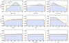 |
Fig. 1. Distribution of each of the model parameters of the full set of model SEDs (solid orange lines), the subset of SEDs for which the size of the corona is smaller than the height of the source (dotted black lines), and of the selected subset of SEDs that agree with the observed L2 keV − L2500 Å correlation (filled blue histograms). This subsample consists of 28% (42 000 SEDs) of the full set of model SEDs. The dashed green histogram in the upper left panel corresponds to the distribution of log λEdd of the selected subset of model SEDs. |
Range of model parameters we used to compute the model SEDs.
In all cases, we considered a wider range of values than what has been observed in large AGN samples to include AGN with either smaller and/or larger parameters than the observational limits that have been established so far, which might have been missed by surveys so far. Consequently, regarding the accretion rate, most AGN accrete at the ∼0.01 up to 1 of their Eddington limit (at least in the local universe; see e.g. Koss et al. 2022a), and we considered a wider range, between 0.001 and 5 times the Eddington limit. Similarly, most of the nearby AGN host BHs with a mass ∼106 − 109 M⊙ (Koss et al. 2022a), although masses up to ∼1010 M⊙ have been measured in higher-redshift objects (see e.g. Duras et al. 2020). We therefore considered a slightly larger sample of BH masses between 105 − 1011 M⊙. The chosen range of Γ (between 1.4 − 2.5) is driven by the fact that most of the sources reported by Lusso et al. (2020), who analysed a large sample of selected quasars from the Sloan Digital Sky Survey (SDSS), have Γ ≲ 2.5, while most of the sources in the Swift/BAT AGN Spectroscopic Survey (BASS) sample (Ricci et al. 2017; Gupta et al. 2024) have Γ ≳ 1.4. As for the high-energy cut-off in the X-ray spectra of AGN, observations indicate that 100 keV ≲ Ecut ≲ 300 keV (see e.g. Ricci et al. 2018). We investigated a slightly wider range between 50 and 500 keV.
The parameters BH spin, coronal height, Ltransf/Ldisc, inclination, and fcol cannot be easily constrained by observations. One of the objectives of this project is to investigate their distribution for the X-ray disc illumination model to explain the observed UV to X-ray correlation in AGN. For this reason, we considered a uniform distribution of these parameters over all of the possible values for Ltransf/Ldisc, we cannot consider values higher than unity because we assume that the X-ray corona is powered by the accretion process, while fcol cannot be much higher than 2.5 (see e.g. Ross et al. 1992).
As discussed in Sect. 2.2 of Dovčiak et al. (2022), KYNSED computes the corona radius (Rc) a posteriori for a given set of parameters, assuming conservation of energy and photon number. All the assumptions and the method of calculating Rc are detailed in Dovčiak & Done (2016) and Dovčiak et al. (2022). Consequently, a set of parameters can be considered physical only if the corona can fit outside of the event horizon of the BH. In other terms, Rc should be smaller than the difference between the coronal height and the radius of the event horizon. Thus, we selected the SEDs for which this condition is fulfilled, which constitute ∼70% of the original sample (a total of 103 000 SEDs out of 150 000). The parameter distribution of this subset is shown as the dotted histogram in Fig. 1. This figure shows that the distribution of Ltransf/Ldisc, h, and Γ deviates significantly from a uniform distribution. The spin distribution shows a slight deviation. The distribution of all of the other parameters remains consistent with being uniform. The deviations in the distributions arise because if at low heights Ltransf/Ldisc were to be high, this would imply a high luminosity, which requires a large radius. This explains the deficit in low height and high Ltransf/Ldisc. Similarly, for high values of Ltransf/Ldisc, if the corona had a soft X-ray spectrum, this would imply a large radius, which explains the deficit in the distribution at high values of Γ.
For each of the model SEDs for which the corona radius was physical, we computed the monochromatic luminosity at 2 keV and 2500 Å (L2 keV and L2500 Å, respectively), the total observed luminosity (Lbol, by integrating the SED between ∼20 μm and 1000 keV), the 2 − 10 keV luminosity (L2-10 keV), and λEdd = Lbol/LEdd, which we refer to as the Eddington ratio. We note that λEdd differs from ṁ/ṁEdd depending on the disc inclination angle. This connection is further explored in Appendix A. The grey dots in Fig. 2 show log L2 keV as a function of the corresponding log L2500 Å for the 150 000 model SEDS. Clearly, under the hypothesis of a uniform distribution of the physical parameters, the X-ray disc illumination predicts that L2 keV increases proportionally with L2500 Å, and the slope of the correlation between log L2 keV and log L2500 Å is expected to be ∼1.
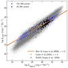 |
Fig. 2. X-ray luminosity vs. UV luminosity for the full set of model SEDs for which the corona radius is physical (grey points; see Sect. 2 for more details). The black points correspond to the data obtained from Lusso et al. (2020) for quasars at a redshift below 2. The orange line shows the best-fit straight line fitted to the black points. The blue points correspond to the model SEDs that are consistent with the best-fit line within 2σ. The white diamonds indicate the data from the BASS sample (Gupta et al. 2024). |
3. The observed L2 keV − L2500 Å correlation
We accept the results of Lusso et al. (2020) as being representative of the UV to X-ray correlation in AGN. Lusso et al. (2020) presented a sample of quasars up to z ∼ 7 where the intrinsic L2500 Å and L2 keV could both be measured. The sources were chosen to show low levels of dust reddening, host galaxy contamination, X-ray absorption, or Eddington bias effects, as discussed in their Sect. 7. In order to avoid any inaccuracy in estimating the intrinsic luminosity due to the assumed cosmology, we only considered sources a redshift below 2 from the clean sample of Lusso et al. (2020).
We used the standard ordinary least-squares method (OLS(Y|X)) from Isobe et al. (1990) to fit a straight line (ymodel = β + γx) to these sources in the log L2 keV − log L2500 Å plane. We normalised the fit at log L2500 Å = 30.5. This resulted in a slope γ = 0.631 ± 0.012 and in a normalisation of β = 26.576 ± 0.007. The scatter4 of the data points around the best-fit line is σ = 0.24 dex. The data from Lusso et al. (2020) and the best-fit line are shown in Fig. 2 as black dots and a solid orange line, respectively.
The white diamonds in the same figure show the (L2 keV, L2500 Å) data for type 1 sources from the BASS sample (Gupta et al. 2024). Clearly, the X-ray/UV data for the unobscured AGN in the nearby Universe agree with the data for the distant quasars. They also appear to be consistent with the best-fit orange line, and their scatter around this line is similar to the scatter of the Lusso et al. (2020) points. The Lusso et al. (2020) and the BASS sample data points in Fig. 2 indicate that the X-ray/UV correlation in AGN, as defined by the orange line in this figure, extends over (at least) five orders of magnitude in UV luminosity, from ∼27 to 32 in log L2500 Å.
Interestingly, the observed data points appear to be a subset of the model data points. We note that there was no reason, a priori, for this agreement between the model and the data. However, it is clear that the slope of the best-fit line to observed log L2 keV − log L2500 Å data deviates from the slope of one that is expected in the case of the X-ray disc reflection model if the parameters were uniformly distributed, as indicated by the orange histograms in Fig. 1.
In the following section, we investigate which subset of the parameter space can produce the observed L2 keV − L2500 Å correlation within the framework of our model. To do this, we selected the model data points in Fig. 2 that were consistent within 2σ with the best-fit line to the data. These model points, indicated by the blue points in the same figure, constitute 28% of the full set of simulated SEDs (42 000 SEDs out of the original 150 000 simulated ones). We considered all the points over the full range of the X-ray and UV luminosity resulting from the model SEDs. This exceeds the range of the X-ray and UV luminosity sampled by the BASS and the Lusso et al. (2020) observations, but we kept the full range in case the observations so far have not revealed the full population of AGN. We note that choosing points with any scatter smaller than 3σ around the best fit does not affect the conclusions of our results (see Sect. 6.1 for more details).
In the following section, we consider the model parameters that correspond to the X-ray and UV luminosity pairs indicated by the blue points in Fig. 2. Our objective is to investigate their distribution and potential correlations, which are necessary to explain the observed L2 keV − L2500 Å correlation.
4. The model parameters that can explain the observed UV to X-ray correlation
The filled blue histograms in Fig. 1 show the distribution of the parameters for the selected subset of model SEDs that are consistent with the observed L2 keV − L2500 Å correlation. The parameter distributions of this subset agree with the original distributions (dotted histograms in Fig. 1), except for log MBH, log ṁ/ṁEdd, and Ltransf/Ldisc. The new distribution of log MBH/M⊙ shows a broad peak at ∼8.5 − 10. The abrupt cuts at 5 and 11 are due to the limits we assumed for the original set of model SEDs. The distribution of Ltransf/Ldisc deviates from the original distribution at low values (below ∼0.4), where a peak can be seen at 0.2. The distribution of log ṁ/ṁEdd deviates most from the original uniform distribution. It shows a clear peak at accretion rates log ṁ/ṁEdd between ∼ − 1 and −0.5 (as before with the BH mass distribution, the abrupt cuts at −3 and 0.7 are the limits we originally set for the model SEDs). The dashed green line in the top left panel in Fig. 1 shows the resulting distribution for log λEdd. It is very similar to the log ṁ/ṁEdd distribution, but it declines more gradually towards very high and low values (i.e. beyond log λEdd of 0.5 and −3, respectively).
Figure 3 shows the 2D histogram of the accretion rate versus BH mass and of Ltransf/Ldisc versus accretion rate and BH mass (left, middle, and right panel, respectively). The colour scheme was chosen so that the intensity of the bins increases with the number of model points in each bin. In order to better illustrate the correlation between the various parameters, we considered the distribution of log ṁ/ṁEdd (left panel) and Ltransf/Ldisc (middle and right panels) in narrow bins along the x-axis. The filled circles indicate the median value in each bin. The open diamonds show the same but considering log λEdd instead of log ṁ/ṁEdd. Because the distributions in each bins may not be symmetric, we also show the mode of the distributions as solid white lines. Clear correlations can be seen between all three parameters. The left panel shows that ṁ/ṁEdd decreases with increasing BH mass. As for Ltransf/Ldisc, the middle panel shows that it remains relatively constant at ∼0.4 − 0.5 on average for log ṁ/ṁEdd ≲ −1, and then it decreases with increasing accretion rates. On the other hand, Ltransf/Ldisc does not appear to be correlated with BH mass up to log MBH ∼ 9. At higher BH masses, Ltransf/Ldisc decreases with increasing BH mass. The mode of the distribution agrees perfectly with the median in the left panel. In the middle and right panel, the trends seen in the mode and median are similar in shape, but with a difference in the amplitude, which is due to the asymmetry of the distributions.
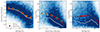 |
Fig. 3. Correlation between log ṁ/ṁEdd and log MBH, Ltransf/Ldisc and log ṁ/ṁEdd, and between Ltransf/Ldisc and log MBH (left, middle, and right panels, respectively) for the subset of model SEDs that are consistent with the observed L2 keV − L2500 Å correlation. The blue squares correspond to the 2D histograms. The red circles correspond to the median parameters in narrow bins along the x-axis. The empty diamonds show the median log λEdd, computed in the same bins. The solid white lines show the mode of the distribution in each of the bins along the x-axis. |
Our main result so far is that the observed correlation between the X-ray and UV luminosity is a generic feature of the X-ray illumination of the accretion disc model. When we assume that this correlation extends over the full luminosity range, as indicated by the blue points in Fig. 2, then it can be reproduced as long as (a) the distributions of MBH, ṁ/ṁEdd, and Ltransf/Ldisc follow the blue histograms in Fig. 1, and (b) ṁ/ṁEdd correlates with MBH and Ltransf/Ldisc correlates with ṁ/ṁEdd and MBH as shown in Fig. 3.
5. Observational validity tests of the predictions from the X-ray disc illumination model
The agreement between the model and the observed L2 keV − L2500 Å correlation does not prove that the X-ray disc illumination model is indeed correct for AGN. However, our results imply that the X-ray disc illumination model can explain the observed correlation only if certain correlations exist between the accretion rate, BH mass, and Ltransf/Ldisc. These correlations are specific to the X-ray illumination model. We do not expect AGN to necessarily follow these correlations if other models can reproduce the observed L2 keV − L2500 Å correlation in these objects.
For this reason, we present below the results from the comparison between the model specific predictions (shown in Fig. 3) with observations. In particular, we considered the physical parameters for the model SEDs for which L2 keV and L2500 Å agree with the observed correlation in AGN. As we already mentioned, there is no reason, a priori, why the correlation that the model predicts between physical parameters such as ṁ/ṁEdd and MBH agree with the corresponding observed correlations if a different physical mechanism can reproduce the UV/X-ray correlation in AGN. Thus, the observational tests we present in the following are independent ways to investigate the validity of the X-ray disc illumination model.
5.1. Observational evidence for the λEdd versus MBH relation in AGN
The Eddington ratio is one of the key AGN properties because it helps us to understand the accretion process, and it is a crucial parameter for AGN feedback. In Fig. 4 we show the distribution of λEdd as a function of MBH in the selected subset of model SEDs that agree with the observed L2 keV − L2500 Å correlation. Instead of showing the data points themselves, we show in this figure contours that encompass 68%, 95%, and 99% of our model data.
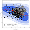 |
Fig. 4. Eddington ratio vs. black hole mass for the subset of model SEDs that agree with the L2 keV − L2500 Å correlation. The shaded darker to lighter blue contours correspond to 68%, 95%, and 99% of the model data points. We also show the observed data from Lusso et al. (2020, grey stars) and from the BASS sample (only type 1 sources; black diamonds). The connected red and white diamonds indicate the median data from the subsample of SEDs that agree with the observed L2 keV − L2500 Å correlation and those from the BASS sample, respectively. |
The grey stars in this figure show the (log MBH, log λEdd) data points for the quasars in Lusso et al. (2020) with z < 2. For these sources, we considered the corresponding MBH and λEdd from Wu & Shen (2022), who provided measurements of various quasar properties from the SDSS data release 16. Clearly, the Lusso et al. (2020) quasars fully agree with the model predictions because the majority of the sources lies within the 68% contour of the model data.
We also compared our results with data from other recent AGN surveys. For example, the black diamonds in Fig. 4 show the (log MBH, log λEdd) data for type 1 AGN from the Swift/BAT AGN Spectroscopic Survey (BASS; Koss et al. 2017, 2022a,b). This is a hard X-ray selected sample that may not be affected by strong selection effects, and it is representative of the AGN population in the local Universe. We only show data for the type 1 objects to be able to compare them with results from other samples that mainly consist of type 1 AGN. In any case, type 1 sources are preferable, as our modelling does not account for absorption. Figure 4 shows that the majority of the BASS data are consistent with the 68% contour of our model prediction. Furthermore, the white diamonds in this figure indicate the mean log λEdd versus log MBH relation in the BASS data, which shows the same shape as the relation predicted by our model (red diamonds in the same figure). The difference in amplitude between the white and red diamonds arises from the selection effects that might be present in the BASS sample, especially because BASS is less sensitive to sources with high Eddington ratios, as they tend to have softer X-ray spectra.
The results in this section indicate that a relation between the accretion rate and the BH mass exists for the quasars in the Lusso et al. (2020) sample that we used to define the L2 keV − L2500 Å relation, and for other samples as well. In all cases, this relation is entirely consistent with the predictions of the disc X-ray illuminated model. We investigate below additional observational evidence that shows that AGN are also consistent with the other model requirements to explain the observed L2 keV − L2500 Å relation, that is, the Ltransf/Ldisc versus ṁ/ṁEdd and MBH correlations shown in the middle and right panels in Fig. 3.
5.2. Observational evidence for the Ltransf/Ldisc–ṁ/ṁEdd and Ltransf/Ldisc–MBH relations in AGN
As we already mentioned, it is difficult to measure Ltransf/Ldisc in AGN from observations. However, it is rather trivial to determine the 2 − 10 keV luminosity in these objects, and consequently, the X-ray bolometric correction (k2 − 10 = Lbol/L2-10 keV). These two quantities are expected to be negatively correlated because Ltransf/Ldisc represents the ratio of the X-ray luminosity to the accretion luminosity. Figure 5 shows that this negative correlation is indeed seen in the model SEDs that agree with the observed L2 keV–L2500 Å correlation. We fit this correlation in the log-space and found a slope of −0.9. We note that the same correlation was found when we considered the full set of model SEDs. Thus, we use k2−10 in this section as a proxy for Ltransf/Ldisc to test the dependence on mass and accretion rate.
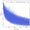 |
Fig. 5. X-ray bolometric correction as a function of Ltransf/Ldisc for the subset of model SEDs that agree with the observed L2 keV–L2500 Å correlation. The red line shows the best-fit line to this correlation. |
In Fig. 6 we show k2−10 as a function of MBH and λEdd for the type 1 AGN observed in the BASS sample (Gupta et al. 2024). As mentioned earlier, we expect the dependence of k2−10 on λEdd and MBH to be consistent with the dependences shown in the middle and right panel of Fig. 3. Thus, for the MBH range probed by BASS (log MBH ∼ 6 − 9), we do not expect to see any change in k2−10. However, we expect k2−10 to increase with λEdd (k2−10 being inversely proportional to Ltransf/Ldisc). The black circles in this figure correspond to the binned BASS data along the x-axes, and they show similar trends to the expected trend, but with relatively large scatter. The red diamonds in this figure show the same quantities from the model SEDs that agree with the observed L2−10 keV–L2500 Å correlation, considering a similar binning. These points were obtained by selecting the model SEDs that match the observed MBH and λEdd distributions from the BASS sample. Our model values and those observed in the BASS sample clearly agree in this figure. In Appendix B we show the dependence of the 2 − 10 keV luminosity on the BH mass, accretion rate, and Ltransf/Ldisc. This is another way of quantifying the effects discussed in this section.
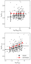 |
Fig. 6. X-ray bolometric correction as a function of MBH (top) and λEdd (bottom). The grey circles correspond to the data points from BASS (Gupta et al. 2024). The black circles show the same data, but binned along the x-axis. We also show k2−10 as a function of MBH and λEdd for the model SEDs that agree with the observed L2−10 keV–L2500 Å correlation obtained by matching the distributions of MBH and λEdd to those of the BASS sample (red diamonds). |
6. Discussion and conclusions
In summary, we used the KYNSED model, which assumes an X-ray illumination of accretion disc, to estimate 150 000 pairs of AGN X-ray and UV luminosity data points for a wide range of physical parameters, assuming a uniform distribution of a reasonable range of values. We found that only a sub-sample of the model parameters can predict an X-ray and UV luminosity, in agreement with the observed L2 keV − L2500 Å correlation presented by Lusso et al. (2020). Our results indicate that the observed L2 keV − L2500 Å correlation is a generic feature of the X-ray disc illumination as long as two conditions are fulfilled: (a) MBH, ṁ/ṁEdd, and Ltransf/Ldisc follow the distributions shown in Fig. 1 as blue histograms, and (b) ṁ/ṁEdd is correlated with MBH and Ltransf/Ldisc is correlated with ṁ/ṁEdd and MBH as shown in Fig. 3. In addition, we found evidence that the correlations predicted by our model fully agree with the AGN observations. This further supports the X-ray illuminated disc scenario in AGN. We note that our findings depend on the coronal geometry, which is assumed to be a lamp post in KYNSED. Dovčiak et al. (2022) showed that considering a 3D spherical corona would have a minimum effect compared to a point-source corona. A different coronal geometry (e.g. a radially extended corona) would alter the illumination pattern of the disc, which would modify the disc response and the thermally reprocessed radiation. An investigation of different coronal geometries is beyond the scope of this work. However, we stress that any geometry must be able to explain all of the observed features in AGN, that is, the time lag behaviour as a function of wavelength, the observed variability and correlations between various wavelengths, and the spectral properties.
6.1. Predicted model correlations
The correlations between MBH, ṁ/ṁEdd, and Ltransf/Ldisc presented in Fig. 3 are one of the main predictions of this work. These correlations as well as the distributions of the model parameters (blue histograms in Fig. 1) depend on (a) the choice of the range of each of the parameters in Table 1, and (b) the choice of the 2σ scatter around the best fit (blue points in Fig. 2). While the true range of each of the model parameter values cannot be known a priori, our choice is a good representation of the range of parameters observed in AGN. Regarding the choice of the 2σ scatter around the best-fit L2 keV − L2500 Å correlation, we tested how different values of the scatter might affect the predicted correlations.
In the left panel of Fig. 7, we show that the average correlation between the three parameters is not affected by the choice of the scatter. We considered a scatter between 0.5σ and 3σ around the best-fit L2 keV − L2500 Å correlation shown in Fig. 2. The correlations clearly become less important as the scatter increases. However, Fig. 7 shows that the predicted correlations do not change much for a scatter below 3σ. This figure shows that our choice of the 2σ scatter does not affect the conclusions of this work. Furthermore, it also shows that our conclusions still hold even when the intrinsic scatter around the L2 keV − L2500 Å correlation is very small. Some works have argued that the dispersion in the log L2 keV − log L2500 Å correlation might be much smaller than the value of ∼0.24 dex found by Lusso et al. (2020) (see e.g. Sacchi et al. 2022; Signorini et al. 2024). In the right panel of Fig. 7, we show the 1D distribution of MBH, ṁ/ṁEdd, and Ltransf/Ldisc for the model SEDs that agree with the observed L2 keV − L2500 Å correlation assuming a scatter around of the best fit below 3σ. This shows that the distributions of the parameters are not highly affected by the choice of the scatter as long as it is below 3σ.
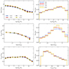 |
Fig. 7. Left: Average correlations between log ṁ/ṁEdd, log MBH, and Ltransf/Ldisc, similar to Fig. 3 considering different values of the scatter around the best-fit L2 keV–L2500 Å correlation ranging between 0.5σ and 3σ. Right: Distribution of log MBH, log ṁ/ṁEdd, and Ltransf/Ldisc (top to bottom) for the selected subset of SEDs that agree with the observed L2 keV − L2500 Å correlation assuming a scatter around the best fit between 0.5σ and 3σ. |
6.2. Independent additional tests
The quasars from the Lusso et al. (2020) sample that we used to define the observed L2 keV − L2500 Å correlation follow the λEdd − MBH correlation (and consequently, the ṁ/ṁEdd − MBH correlation) predicted by our model, as shown in Fig. 4. The agreement between our model predictions and observed data also applies to all of the samples we considered in Sect. 5. In particular, the agreement between our model predictions and the BASS sample is a strong validation of our model because this sample is assumed to be representative of the total population of AGN in the local Universe. Furthermore, we showed in Sect. 5.2 that our model predicts a specific dependence of k2−10 on MBH and λEdd that agrees with the trends observed in the BASS sample. As we mentioned in this section, the correlation is a proxy for the Ltransf/Ldisc–MBH and Ltransf/Ldisc–ṁ/ṁEdd correlations. Observations of AGN samples result in correlations that completely agree with the correlation predicted by our model. This further supports the X-ray illuminated disc scenario in AGN.
6.3. Implications of the MBH, ṁ/ṁEdd, and Ltransf/Ldisc correlations
The correlation between MBH and ṁ/ṁEdd can be explained in the context of BH growth via accretion. Various works showed that the accretion episode of an SMBH starts with a high accretion rate (in units of Eddington) that decreases as the BH grows in mass and consumes its reservoir (see e.g. Granato et al. 2001, 2004; Merloni 2004; Lapi et al. 2006). These models have been proposed to explain the observational properties of different types of quasars and the co-evolution of SMBHs and their host galaxies (e.g. Kawakatu et al. 2003, 2007). It is worth noting that Lusso et al. (2020) showed that the L2 keV − L2500 Å correlation is valid in all of the redshift ranges probed in their study (see their Fig. 8 and Appendix B). This means that the correlations we predict between MBH, ṁ/ṁEdd, and Ltransf/Ldisc are probably valid in all redshift ranges as well, and consequently, in all evolutionary stages of the sources (if quasars were to grow just via accretion). We note that our model does not consider AGN feedback, which might also affect the SMBH evolution and the observed properties of AGN.
The correlation between Ltransf/Ldisc and ṁ/ṁEdd must be indicative of the unknown physical mechanism that powers the X-ray corona. Our model predicts that the fraction of power transferred to the X-ray corona compared to the disc power decreases at high accretion rates. This behavior is consistent with what is expected in the case of a magnetic reconnection-heated corona scenario (see for example Fig. 3 in Liu et al. 2016). This is also supported by results from studying X-ray bolometeric corrections in sample of AGN, which showed that the X-ray to bolometric luminosity fraction decreases at high luminosity (see e.g. Lusso et al. 2012; Duras et al. 2020).
In conclusion, we showed that the X-ray illumination of accretion discs explains the observed correlation between the X-rays and UV in AGN. Our results also shed light on the physical properties and the evolution of AGN, as we predicted very specific correlations between the BH mass, accretion rate, and Ltransf/Ldisc that are needed to produce the observed L2 keV − L2500 Å correlation in AGN. All of these model predictions agree with the observations of a large sample of AGN.
Data availability
The data that support the findings of this study are available from the corresponding author, EK, upon reasonable request.
Rg = GMBH/c2 is the gravitational radius of a BH with a mass of MBH.
We produce the model SEDs using PyXSPEC, the Python interface of XSPEC Arnaud (1996).
We calculate the scatter as  .
.
Acknowledgments
We thank the anonymous referee for their constructive feedback. EK and IEP acknowledge support from the European Union’s Horizon 2020 Programme under the AHEAD2020 project (grant agreement n. 871158). Software packages used in this study include XSPEC/PyXSPEC (Arnaud 1996), NumPy (Harris et al. 2020), SciPy (Virtanen et al. 2020), Pandas (McKinney 2010), Matplotlib (Hunter 2007), and GetDist (Lewis 2019).
References
- Arnaud, K. A. 1996, ASP Conf. Ser., 101, 17 [Google Scholar]
- Avni, Y., & Tananbaum, H. 1982, ApJ, 262, L17 [NASA ADS] [CrossRef] [Google Scholar]
- Avni, Y., & Tananbaum, H. 1986, ApJ, 305, 83 [Google Scholar]
- De Rosa, G., Peterson, B. M., Ely, J., et al. 2015, ApJ, 806, 128 [NASA ADS] [CrossRef] [Google Scholar]
- Dovčiak, M., & Done, C. 2016, Astron. Nachr., 337, 441 [CrossRef] [Google Scholar]
- Dovčiak, M., Papadakis, I. E., Kammoun, E. S., & Zhang, W. 2022, A&A, 661, A135 [NASA ADS] [CrossRef] [EDP Sciences] [Google Scholar]
- Duras, F., Bongiorno, A., Ricci, F., et al. 2020, A&A, 636, A73 [NASA ADS] [CrossRef] [EDP Sciences] [Google Scholar]
- Galeev, A. A., Rosner, R., & Vaiana, G. S. 1979, ApJ, 229, 318 [NASA ADS] [CrossRef] [Google Scholar]
- Granato, G. L., Silva, L., Monaco, P., et al. 2001, MNRAS, 324, 757 [Google Scholar]
- Granato, G. L., De Zotti, G., Silva, L., Bressan, A., & Danese, L. 2004, ApJ, 600, 580 [Google Scholar]
- Gupta, K. K., Ricci, C., Temple, M. J., et al. 2024, A&A, 691, A203 [NASA ADS] [CrossRef] [EDP Sciences] [Google Scholar]
- Haardt, F., Maraschi, L., & Ghisellini, G. 1994, ApJ, 432, L95 [NASA ADS] [CrossRef] [Google Scholar]
- Harris, C. R., Millman, K. J., van der Walt, S. J., et al. 2020, Nature, 585, 357 [NASA ADS] [CrossRef] [Google Scholar]
- Hunter, J. D. 2007, Comput. Sci. Eng., 9, 90 [NASA ADS] [CrossRef] [Google Scholar]
- Isobe, T., Feigelson, E. D., Akritas, M. G., & Babu, G. J. 1990, ApJ, 364, 104 [Google Scholar]
- Jin, C., Lusso, E., Ward, M., Done, C., & Middei, R. 2024, MNRAS, 527, 356 [Google Scholar]
- Kammoun, E. S., Papadakis, I. E., & Dovčiak, M. 2019, ApJ, 879, L24 [NASA ADS] [CrossRef] [Google Scholar]
- Kammoun, E. S., Dovčiak, M., Papadakis, I. E., Caballero-García, M. D., & Karas, V. 2021a, ApJ, 907, 20 [NASA ADS] [CrossRef] [Google Scholar]
- Kammoun, E. S., Papadakis, I. E., & Dovčiak, M. 2021b, MNRAS, 503, 4163 [CrossRef] [Google Scholar]
- Kammoun, E. S., Robin, L., Papadakis, I. E., Dovčiak, M., & Panagiotou, C. 2023, MNRAS, 526, 138 [NASA ADS] [CrossRef] [Google Scholar]
- Kammoun, E., Papadakis, I. E., Dovčiak, M., & Panagiotou, C. 2024, A&A, 686, A69 [NASA ADS] [CrossRef] [EDP Sciences] [Google Scholar]
- Kawakatu, N., Umemura, M., & Mori, M. 2003, ApJ, 583, 85 [NASA ADS] [CrossRef] [Google Scholar]
- Kawakatu, N., Imanishi, M., & Nagao, T. 2007, ApJ, 661, 660 [Google Scholar]
- Koss, M., Trakhtenbrot, B., Ricci, C., et al. 2017, ApJ, 850, 74 [Google Scholar]
- Koss, M. J., Ricci, C., Trakhtenbrot, B., et al. 2022a, ApJS, 261, 2 [NASA ADS] [CrossRef] [Google Scholar]
- Koss, M. J., Trakhtenbrot, B., Ricci, C., et al. 2022b, ApJS, 261, 1 [NASA ADS] [CrossRef] [Google Scholar]
- Kriss, G. A., & Canizares, C. R. 1985, ApJ, 297, 177 [Google Scholar]
- Langis, D. A., Papadakis, I. E., Kammoun, E., Panagiotou, C., & Dovčiak, M. 2024, A&A, 691, A252 [NASA ADS] [CrossRef] [EDP Sciences] [Google Scholar]
- Lapi, A., Shankar, F., Mao, J., et al. 2006, ApJ, 650, 42 [Google Scholar]
- Lewis, A. 2019, ArXiv e-prints [arXiv:1910.13970] [Google Scholar]
- Liu, J. Y., Qiao, E. L., & Liu, B. F. 2016, ApJ, 833, 35 [NASA ADS] [CrossRef] [Google Scholar]
- Lusso, E., & Risaliti, G. 2016, ApJ, 819, 154 [Google Scholar]
- Lusso, E., Comastri, A., Vignali, C., et al. 2010, A&A, 512, A34 [NASA ADS] [CrossRef] [EDP Sciences] [Google Scholar]
- Lusso, E., Comastri, A., Simmons, B. D., et al. 2012, MNRAS, 425, 623 [Google Scholar]
- Lusso, E., Risaliti, G., Nardini, E., et al. 2020, A&A, 642, A150 [NASA ADS] [CrossRef] [EDP Sciences] [Google Scholar]
- McKinney, W. 2010, in Proceedings of the 9th Python in Science Conference, eds. S. van der Walt, & J. Millman, 56 [Google Scholar]
- Merloni, A. 2004, MNRAS, 353, 1035 [NASA ADS] [CrossRef] [Google Scholar]
- Novikov, I. D., & Thorne, K. S. 1973, in Black Holes (Les Astres Occlus), eds. C. Dewitt, & B. S. Dewitt, 343 [Google Scholar]
- Panagiotou, C., Papadakis, I. E., Kammoun, E. S., & Dovčiak, M. 2020, MNRAS, 499, 1998 [CrossRef] [Google Scholar]
- Panagiotou, C., Papadakis, I., Kara, E., Kammoun, E., & Dovčiak, M. 2022, ApJ, 935, 93 [NASA ADS] [CrossRef] [Google Scholar]
- Papadakis, I. E., Dovčiak, M., & Kammoun, E. S. 2022, A&A, 666, A11 [Google Scholar]
- Papoutsis, M., Papadakis, I. E., Panagiotou, C., Dovčiak, M., & Kammoun, E. 2024, A&A, 691, A60 [NASA ADS] [CrossRef] [EDP Sciences] [Google Scholar]
- Ricci, C., Trakhtenbrot, B., Koss, M. J., et al. 2017, ApJS, 233, 17 [Google Scholar]
- Ricci, C., Ho, L. C., Fabian, A. C., et al. 2018, MNRAS, 480, 1819 [NASA ADS] [CrossRef] [Google Scholar]
- Ross, R. R., Fabian, A. C., & Mineshige, S. 1992, MNRAS, 258, 189 [NASA ADS] [CrossRef] [Google Scholar]
- Sacchi, A., Risaliti, G., Signorini, M., et al. 2022, A&A, 663, L7 [NASA ADS] [CrossRef] [EDP Sciences] [Google Scholar]
- Shields, G. A. 1978, Nature, 272, 706 [NASA ADS] [CrossRef] [Google Scholar]
- Signorini, M., Risaliti, G., Lusso, E., et al. 2023, A&A, 676, A143 [NASA ADS] [CrossRef] [EDP Sciences] [Google Scholar]
- Signorini, M., Risaliti, G., Lusso, E., et al. 2024, A&A, 687, A32 [NASA ADS] [CrossRef] [EDP Sciences] [Google Scholar]
- Steffen, A. T., Strateva, I., Brandt, W. N., et al. 2006, AJ, 131, 2826 [Google Scholar]
- Strateva, I. V., Brandt, W. N., Schneider, D. P., Vanden Berk, D. G., & Vignali, C. 2005, AJ, 130, 387 [Google Scholar]
- Tananbaum, H., Avni, Y., Branduardi, G., et al. 1979, ApJ, 234, L9 [Google Scholar]
- Vignali, C., Brandt, W. N., & Schneider, D. P. 2003, AJ, 125, 433 [Google Scholar]
- Virtanen, P., Gommers, R., Oliphant, T. E., et al. 2020, Nat. Meth., 17, 261 [Google Scholar]
- Wilkes, B. J., Tananbaum, H., Worrall, D. M., et al. 1994, ApJS, 92, 53 [NASA ADS] [CrossRef] [Google Scholar]
- Wu, Q., & Shen, Y. 2022, ApJS, 263, 42 [NASA ADS] [CrossRef] [Google Scholar]
- Young, M., Elvis, M., & Risaliti, G. 2010, ApJ, 708, 1388 [Google Scholar]
Appendix A: The connection between the Eddington ratio and the accretion rate
In this section we explore the connection between ṁ/ṁEdd and λEdd. Within KYNSED, ṁ/ṁEdd is accretion rate normalized to the Eddington accretion rate. The accretion power is computed self-consistently within the code by considering the radiative efficiency (η), which is a function of the BH spin ( ). If the emission were to be isotropic, ṁ/ṁEdd should be equal to λEdd. However, since we see a dependence on the inclination angle as shown in the left panel Fig. A.1. We see a non-symmetric and relatively large scatter compared to the 1:1 correlation. To quantify the dependence on inclination, we divided the points into bins of cos i with a width of 0.01. Then we fitted log ṁ/ṁEdd vs log λEdd in each bin with a straight line. As expected, the best-fit slopes are consistent with 1 for all the bins, with an average value of 0.997. However, the normalizations vary as a function of inclination. We fitted the normalization as a function of cos i with a phenomenological polynomial of degree three:
 (A.1)
(A.1)
where μ = cos i. When we add the effect of inclination, the scatter becomes symmetric and reduces to 0.03 dex. Thus, based on our model, for a given inclination angle, the relation between ṁ/ṁEdd and λEdd can be described as
 (A.2)
(A.2)
Thus, for a given source, knowing the value of λEdd based on observations, the above equations could be used to estimate the accretion rate assuming a certain inclination angle.
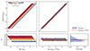 |
Fig. A.1. Left: Accretion rate (log ṁ/ṁEdd) as a function of the Eddington ratio (log λEdd). The solid line show the identity line. The bottom panel shows the difference between log ṁ/ṁEdd and the identity line. Middle: Same but replacing the x-axis with the sum of log λEdd and a polynomial function of the inclination angle to account for the anisotropy in the emission (see text for more details). The colour maps corresponds to μ = cos i. Bottom right: Distribution of the differences between the y-axis and the x-axis in the left and middle panels (blue and red histograms, respectively) |
Appendix B: Observational evidence for the L2−10 keV-MBH-ṁ/ṁEddelations in AGN
In this section we investigate whether there is a correlation between L2−10 keV and ṁ/ṁEdd/MBH in the model SEDs which are consistent with the observed L2 keV − L2500 Å correlation in AGN. To this end, we fitted log L2-10 keV as a linear combination of log MBH and log λEdd using the Scipy function curve_fit5. The best-fit correlation obtained can be written as follows:
 (B.1)
(B.1)
Figure B.1 shows log L2-10 keV plotted as a function of the best-fit linear relation defined by this correlation. Clearly, the X-ray illuminated disc model predicts a very strong correlation between L2−10 keV and MBH/λEdd in AGN, with a 1σ scatter of 0.26 dex around the best fit. The colour map in this figure shows the distribution of Ltransf/Ldisc. Roughly speaking, AGN with larger Ltransf/Ldisc should be above the dashed line in this plot, while AGN with smaller Ltransf/Ldisc should be below.
 |
Fig. B.1. X-ray luminosity as a function of the BH mass and Eddington ratio for the subset of model SEDs that agree with the observed L2 keV-L2500 Å correlation. Colour maps show the distribution in Ltransf/Ldisc. Each of the panels show the data points from the observed samples we consider in this work. |
We also show in Fig. B.1 the correlation between the observed X-ray luminosity versus the correlation with MBH and λEdd we found in Eq.(B.1) using available data from the different samples we considered in the previous section. Clearly, the observed correlation agrees extremely well with the model predictions. The top right panel shows the data from the Type 1 sources of the BASS sample by Ricci et al. (2017) and revised by Gupta et al. (2024). Interestingly, the majority of these sources fall above the blue line, in agreement with high Ltransf/Ldisc values. This is also the case for the data from Lusso et al. (2010) and Duras et al. (2020), shown in the bottom right panel. As these three samples are X-ray selected, it is thus most likely that they are biased towards high values of Ltransf/Ldisc, where the X-ray power is larger. In fact, X-ray selected samples tend to show an X-ray bolometric correction of the order of ∼10 − 30, which indeed corresponds to high values of Ltransf/Ldisc from Fig. 5. The bottom left panel of this figure shows the data points obtained by Lusso et al. (2020). These data points fill a larger scatter around the best fit compared to the other samples.
We note that, in general, a correlation between between the X-ray luminosity and MBH as well as ṁ/ṁEdd should be expected for any model that predicts the observed L2 keV − L2500 Å correlation in AGN. After all, the 2 keV luminosity is tightly correlated with L2−10 keV, while L2500 Å depends on MBH and ṁ/ṁEdd. However, in the X-ray illuminated disc model, the source of heating for the inner accretion disc is the absorbed X-rays, which are not exactly equal to the accretion power that is transferred to the corona. Therefore, according to the model, L2500 Å should also depend on Ltransf/Ldisc itself. Consequently, the model correlation plotted in Fig. B.1 is very specific to our model, and is representative of the X-ray illuminated disc but only for the model parameters which can explain the UV to X-ray correlation in AGN.
All Tables
All Figures
|
Fig. 1. Distribution of each of the model parameters of the full set of model SEDs (solid orange lines), the subset of SEDs for which the size of the corona is smaller than the height of the source (dotted black lines), and of the selected subset of SEDs that agree with the observed L2 keV − L2500 Å correlation (filled blue histograms). This subsample consists of 28% (42 000 SEDs) of the full set of model SEDs. The dashed green histogram in the upper left panel corresponds to the distribution of log λEdd of the selected subset of model SEDs. |
| In the text | |
|
Fig. 2. X-ray luminosity vs. UV luminosity for the full set of model SEDs for which the corona radius is physical (grey points; see Sect. 2 for more details). The black points correspond to the data obtained from Lusso et al. (2020) for quasars at a redshift below 2. The orange line shows the best-fit straight line fitted to the black points. The blue points correspond to the model SEDs that are consistent with the best-fit line within 2σ. The white diamonds indicate the data from the BASS sample (Gupta et al. 2024). |
| In the text | |
|
Fig. 3. Correlation between log ṁ/ṁEdd and log MBH, Ltransf/Ldisc and log ṁ/ṁEdd, and between Ltransf/Ldisc and log MBH (left, middle, and right panels, respectively) for the subset of model SEDs that are consistent with the observed L2 keV − L2500 Å correlation. The blue squares correspond to the 2D histograms. The red circles correspond to the median parameters in narrow bins along the x-axis. The empty diamonds show the median log λEdd, computed in the same bins. The solid white lines show the mode of the distribution in each of the bins along the x-axis. |
| In the text | |
|
Fig. 4. Eddington ratio vs. black hole mass for the subset of model SEDs that agree with the L2 keV − L2500 Å correlation. The shaded darker to lighter blue contours correspond to 68%, 95%, and 99% of the model data points. We also show the observed data from Lusso et al. (2020, grey stars) and from the BASS sample (only type 1 sources; black diamonds). The connected red and white diamonds indicate the median data from the subsample of SEDs that agree with the observed L2 keV − L2500 Å correlation and those from the BASS sample, respectively. |
| In the text | |
|
Fig. 5. X-ray bolometric correction as a function of Ltransf/Ldisc for the subset of model SEDs that agree with the observed L2 keV–L2500 Å correlation. The red line shows the best-fit line to this correlation. |
| In the text | |
|
Fig. 6. X-ray bolometric correction as a function of MBH (top) and λEdd (bottom). The grey circles correspond to the data points from BASS (Gupta et al. 2024). The black circles show the same data, but binned along the x-axis. We also show k2−10 as a function of MBH and λEdd for the model SEDs that agree with the observed L2−10 keV–L2500 Å correlation obtained by matching the distributions of MBH and λEdd to those of the BASS sample (red diamonds). |
| In the text | |
|
Fig. 7. Left: Average correlations between log ṁ/ṁEdd, log MBH, and Ltransf/Ldisc, similar to Fig. 3 considering different values of the scatter around the best-fit L2 keV–L2500 Å correlation ranging between 0.5σ and 3σ. Right: Distribution of log MBH, log ṁ/ṁEdd, and Ltransf/Ldisc (top to bottom) for the selected subset of SEDs that agree with the observed L2 keV − L2500 Å correlation assuming a scatter around the best fit between 0.5σ and 3σ. |
| In the text | |
|
Fig. A.1. Left: Accretion rate (log ṁ/ṁEdd) as a function of the Eddington ratio (log λEdd). The solid line show the identity line. The bottom panel shows the difference between log ṁ/ṁEdd and the identity line. Middle: Same but replacing the x-axis with the sum of log λEdd and a polynomial function of the inclination angle to account for the anisotropy in the emission (see text for more details). The colour maps corresponds to μ = cos i. Bottom right: Distribution of the differences between the y-axis and the x-axis in the left and middle panels (blue and red histograms, respectively) |
| In the text | |
|
Fig. B.1. X-ray luminosity as a function of the BH mass and Eddington ratio for the subset of model SEDs that agree with the observed L2 keV-L2500 Å correlation. Colour maps show the distribution in Ltransf/Ldisc. Each of the panels show the data points from the observed samples we consider in this work. |
| In the text | |
Current usage metrics show cumulative count of Article Views (full-text article views including HTML views, PDF and ePub downloads, according to the available data) and Abstracts Views on Vision4Press platform.
Data correspond to usage on the plateform after 2015. The current usage metrics is available 48-96 hours after online publication and is updated daily on week days.
Initial download of the metrics may take a while.