| Issue |
A&A
Volume 697, May 2025
Euclid on Sky
|
|
|---|---|---|
| Article Number | A8 | |
| Number of page(s) | 15 | |
| Section | Galactic structure, stellar clusters and populations | |
| DOI | https://doi.org/10.1051/0004-6361/202449696 | |
| Published online | 30 April 2025 | |
Euclid: Early Release Observations – Unveiling the morphology of two Milky Way globular clusters out to their periphery⋆
1
INAF-Osservatorio di Astrofisica e Scienza dello Spazio di Bologna, Via Piero Gobetti 93/3, 40129 Bologna, Italy
2
School of Mathematics and Physics, University of Surrey, Guildford, Surrey, GU2 7XH
UK
3
Leiden Observatory, Leiden University, Einsteinweg 55, 2333 CC Leiden, The Netherlands
4
Kapteyn Astronomical Institute, University of Groningen, PO Box 800 9700 AV Groningen, The Netherlands
5
David A. Dunlap Department of Astronomy & Astrophysics, University of Toronto, 50 St George Street, Toronto, Ontario, M5S 3H4
Canada
6
Jodrell Bank Centre for Astrophysics, Department of Physics and Astronomy, University of Manchester, Oxford Road, Manchester, M13 9PL
UK
7
Institute for Astronomy, University of Edinburgh, Royal Observatory, Blackford Hill, Edinburgh, EH9 3HJ
UK
8
Department of Astrophysics/IMAPP, Radboud University, PO Box 9010 6500 GL Nijmegen, The Netherlands
9
International Space University, 1 Rue Jean-Dominique Cassini, 67400 Illkirch-Graffenstaden, France
10
National Astronomical Observatory of Japan, 2-21-1 Osawa, Mitaka, Tokyo, 181-8588
Japan
11
Université de Strasbourg, CNRS, Observatoire astronomique de Strasbourg, UMR 7550, 67000 Strasbourg, France
12
Université Paris-Saclay, Université Paris Cité, CEA, CNRS, AIM, 91191 Gif-sur-Yvette, France
13
Max-Planck-Institut für Astronomie, Königstuhl 17, 69117 Heidelberg, Germany
14
Max Planck Institute for Extraterrestrial Physics, Giessenbachstr. 1, 85748 Garching, Germany
15
ESAC/ESA, Camino Bajo del Castillo, s/n, Urb. Villafranca del Castillo, 28692 Villanueva de la Cañada, Madrid, Spain
16
INAF-Osservatorio Astronomico di Brera, Via Brera 28, 20122 Milano, Italy
17
Dipartimento di Fisica e Astronomia, Università di Bologna, Via Gobetti 93/2, 40129 Bologna, Italy
18
INFN-Sezione di Bologna, Viale Berti Pichat 6/2, 40127 Bologna, Italy
19
INAF-Osservatorio Astronomico di Padova, Via dell’Osservatorio 5, 35122 Padova, Italy
20
Centre National d’Etudes Spatiales – Centre Spatial de Toulouse, 18 Avenue Edouard Belin, 31401 Toulouse Cedex 9, France
21
Universitäts-Sternwarte München, Fakultät für Physik, Ludwig-Maximilians-Universität München, Scheinerstrasse 1, 81679 München, Germany
22
INAF-Osservatorio Astrofisico di Torino, Via Osservatorio 20, 10025 Pino Torinese, TO, Italy
23
Dipartimento di Fisica, Università di Genova, Via Dodecaneso 33, 16146 Genova, Italy
24
INFN-Sezione di Genova, Via Dodecaneso 33, 16146 Genova, Italy
25
Department of Physics “E. Pancini”, University Federico II, Via Cinthia 6, 80126 Napoli, Italy
26
INAF-Osservatorio Astronomico di Capodimonte, Via Moiariello 16, 80131 Napoli, Italy
27
INFN Section of Naples, Via Cinthia 6, 80126 Napoli, Italy
28
Instituto de Astrofísica e Ciências do Espaço, Universidade do Porto, CAUP, Rua das Estrelas, 4150-762 Porto, Portugal
29
Dipartimento di Fisica, Università degli Studi di Torino, Via P. Giuria 1, 10125 Torino, Italy
30
INFN-Sezione di Torino, Via P. Giuria 1, 10125 Torino, Italy
31
Mullard Space Science Laboratory, University College London, Holmbury St Mary, Dorking, Surrey, RH5 6NT
UK
32
INAF-IASF Milano, Via Alfonso Corti 12, 20133 Milano, Italy
33
Institut de Física d’Altes Energies (IFAE), The Barcelona Institute of Science and Technology, Campus UAB, 08193 Bellaterra, Barcelona, Spain
34
Port d’Informació Científica, Campus UAB, C. Albareda s/n, 08193 Bellaterra, Barcelona, Spain
35
Institute for Theoretical Particle Physics and Cosmology (TTK), RWTH Aachen University, 52056 Aachen, Germany
36
INAF-Osservatorio Astronomico di Roma, Via Frascati 33, 00078 Monteporzio Catone, Italy
37
Dipartimento di Fisica e Astronomia “Augusto Righi” – Alma Mater Studiorum Università di Bologna, Viale Berti Pichat 6/2, 40127 Bologna, Italy
38
European Space Agency/ESRIN, Largo Galileo Galilei 1, 00044 Frascati, Roma, Italy
39
Université Claude Bernard Lyon 1, CNRS/IN2P3, IP2I Lyon, UMR 5822, Villeurbanne, 69100
France
40
Institute of Physics, Laboratory of Astrophysics, Ecole Polytechnique Fédérale de Lausanne (EPFL), Observatoire de Sauverny, 1290 Versoix, Switzerland
41
UCB Lyon 1, CNRS/IN2P3, IUF, IP2I Lyon, 4 Rue Enrico Fermi, 69622 Villeurbanne, France
42
Department of Astronomy, University of Geneva, ch. d’Ecogia 16, 1290 Versoix, Switzerland
43
Departamento de Física, Faculdade de Ciências, Universidade de Lisboa, Edifício C8, Campo Grande, 1749-016 Lisboa, Portugal
44
Instituto de Astrofísica e Ciências do Espaço, Faculdade de Ciências, Universidade de Lisboa, Campo Grande, 1749-016 Lisboa, Portugal
45
INFN-Padova, Via Marzolo 8, 35131 Padova, Italy
46
INAF-Istituto di Astrofisica e Planetologia Spaziali, Via del Fosso del Cavaliere, 100, 00100 Roma, Italy
47
INAF-Osservatorio Astronomico di Trieste, Via G. B. Tiepolo 11, 34143 Trieste, Italy
48
Istituto Nazionale di Fisica Nucleare, Sezione di Bologna, Via Irnerio 46, 40126 Bologna, Italy
49
Dipartimento di Fisica “Aldo Pontremoli”, Università degli Studi di Milano, Via Celoria 16, 20133 Milano, Italy
50
INFN-Sezione di Milano, Via Celoria 16, 20133 Milano, Italy
51
Higgs Centre for Theoretical Physics, School of Physics and Astronomy, The University of Edinburgh, Edinburgh, EH9 3FD
UK
52
Jet Propulsion Laboratory, California Institute of Technology, 4800 Oak Grove Drive, Pasadena, CA, 91109
USA
53
Department of Physics, Lancaster University, Lancaster, LA1 4YB
UK
54
von Hoerner & Sulger GmbH, Schlossplatz 8, 68723 Schwetzingen, Germany
55
Technical University of Denmark, Elektrovej 327, 2800 Kgs. Lyngby, Denmark
56
Cosmic Dawn Center (DAWN), Denmark
57
Institut d’Astrophysique de Paris, UMR 7095, CNRS, and Sorbonne Université, 98 Bis boulevard Arago, 75014 Paris, France
58
Department of Physics and Helsinki Institute of Physics, Gustaf Hällströmin katu 2, 00014 University of Helsinki, Finland
59
Aix-Marseille Université, CNRS/IN2P3, CPPM, Marseille, France
60
Université de Genève, Département de Physique Théorique and Centre for Astroparticle Physics, 24 Quai Ernest-Ansermet, 1211 Genève 4, Switzerland
61
Department of Physics, PO Box 64 00014 University of Helsinki, Finland
62
Helsinki Institute of Physics, Gustaf Hällströmin katu 2, University of Helsinki, Helsinki, Finland
63
Institute of Theoretical Astrophysics, University of Oslo, PO Box 1029 Blindern, 0315 Oslo, Norway
64
NOVA optical infrared instrumentation group at ASTRON, Oude Hoogeveensedijk 4, 7991 PD Dwingeloo, The Netherlands
65
Universität Bonn, Argelander-Institut für Astronomie, Auf dem Hügel 71, 53121 Bonn, Germany
66
Aix-Marseille Université, CNRS, CNES, LAM, Marseille, France
67
Dipartimento di Fisica e Astronomia “Augusto Righi” – Alma Mater Studiorum Università di Bologna, Via Piero Gobetti 93/2, 40129 Bologna, Italy
68
Department of Physics, Institute for Computational Cosmology, Durham University, South Road, Durham, DH1 3LE
UK
69
Université Côte d’Azur, Observatoire de la Côte d’Azur, CNRS, Laboratoire Lagrange, Bd de l’Observatoire, CS 34229, 06304 Nice Cedex 4, France
70
Université Paris Cité, CNRS, Astroparticule et Cosmologie, 75013 Paris, France
71
Institut d’Astrophysique de Paris, 98bis Boulevard Arago, 75014 Paris, France
72
European Space Agency/ESTEC, Keplerlaan 1, 2201 AZ Noordwijk, The Netherlands
73
Department of Physics and Astronomy, University of Aarhus, Ny Munkegade 120, 8000 Aarhus C, Denmark
74
Waterloo Centre for Astrophysics, University of Waterloo, Waterloo, Ontario, N2L 3G1
Canada
75
Department of Physics and Astronomy, University of Waterloo, Waterloo, Ontario, N2L 3G1
Canada
76
Perimeter Institute for Theoretical Physics, Waterloo, Ontario, N2L 2Y5
Canada
77
Space Science Data Center, Italian Space Agency, Via del Politecnico snc, 00133 Roma, Italy
78
Institute of Space Science, Str. Atomistilor, nr. 409 Măgurele, Ilfov, 077125
Romania
79
Instituto de Astrofísica de Canarias, Calle Vía Láctea s/n, 38204 San Cristóbal de La Laguna, Tenerife, Spain
80
Departamento de Astrofísica, Universidad de La Laguna, 38206 La Laguna, Tenerife, Spain
81
Dipartimento di Fisica e Astronomia “G. Galilei”, Università di Padova, Via Marzolo 8, 35131 Padova, Italy
82
Departamento de Física, FCFM, Universidad de Chile, Blanco Encalada 2008, Santiago, Chile
83
Universität Innsbruck, Institut für Astro- und Teilchenphysik, Technikerstr. 25/8, 6020 Innsbruck, Austria
84
Institut d’Estudis Espacials de Catalunya (IEEC), Edifici RDIT, Campus UPC, 08860 Castelldefels, Barcelona, Spain
85
Institute of Space Sciences (ICE, CSIC), Campus UAB, Carrer de Can Magrans, s/n, 08193 Barcelona, Spain
86
Satlantis, University Science Park, Sede Bld, 48940 Leioa-Bilbao, Spain
87
Centre for Electronic Imaging, Open University, Walton Hall, Milton Keynes, MK7 6AA
UK
88
Centro de Investigaciones Energéticas, Medioambientales y Tecnológicas (CIEMAT), Avenida Complutense 40, 28040 Madrid, Spain
89
Infrared Processing and Analysis Center, California Institute of Technology, Pasadena, CA, 91125
USA
90
Instituto de Astrofísica e Ciências do Espaço, Faculdade de Ciências, Universidade de Lisboa, Tapada da Ajuda, 1349-018 Lisboa, Portugal
91
Universidad Politécnica de Cartagena, Departamento de Electrónica y Tecnología de Computadoras, Plaza del Hospital 1, 30202 Cartagena, Spain
92
Institut de Recherche en Astrophysique et Planétologie (IRAP), Université de Toulouse, CNRS, UPS, CNES, 14 Av. Edouard Belin, 31400 Toulouse, France
93
INFN-Bologna, Via Irnerio 46, 40126 Bologna, Italy
94
IFPU, Institute for Fundamental Physics of the Universe, Via Beirut 2, 34151 Trieste, Italy
95
INAF, Istituto di Radioastronomia, Via Piero Gobetti 101, 40129 Bologna, Italy
96
California institute of Technology, 1200 E California Blvd, Pasadena, CA, 91125
USA
97
Junia, EPA department, 41 Bd Vauban, 59800 Lille, France
98
Aurora Technology for European Space Agency (ESA), Camino Bajo del Castillo, s/n, Urbanizacion Villafranca del Castillo, Villanueva de la Cañada, 28692 Madrid, Spain
99
Department of Physics and Astronomy, University of British Columbia, Vancouver, BC, V6T 1Z1
Canada
⋆⋆ Corresponding author; davide.massari@inaf.it
Received:
22
February
2024
Accepted:
14
May
2024
As part of the Euclid Early Release Observations (ERO) programme, we analysed deep, wide-field imaging from the VIS and NISP instruments of two Milky Way globular clusters (GCs), namely NGC 6254 (M10) and NGC 6397, to look for observational evidence of their dynamical interaction with the Milky Way. We searched for such an interaction in the form of structural and morphological features in the clusters’ outermost regions, which would be suggestive of the development of tidal tails on scales larger than those sampled by the ERO data. From our multi-band photometric analysis, we obtained deep and well-behaved colour–magnitude diagrams that, in turn, enabled an accurate membership selection. The surface brightness profiles built from these samples of member stars are the deepest ever obtained for these two Milky Way GCs, reaching down to ∼30.0 mag/arcsec2, which is ∼1.5 mag/arcsec2 lower than before. The investigation of the two-dimensional density map of NGC 6254 reveals an elongated morphology of the cluster peripheries in the direction and with the amplitude predicted by N-body simulations of the cluster’s dynamical evolution, at high statistical significance. We interpret this as strong evidence for the first detection of tidally induced morphological distortion around this cluster. The density map of NGC 6397 reveals a slightly elliptical morphology, in agreement with previous studies, which requires further investigation on larger scales to be properly interpreted. This ERO project thus demonstrates the power of Euclid in studying the outer regions of GCs at an unprecedented level of detail, thanks to the combination of the large field of view, high spatial resolution, and depth enabled by the telescope. Our results highlight the future Euclid survey as the ideal dataset for investigating GC tidal tails and stellar streams.
Key words: stars: imaging / Galaxy: evolution / globular clusters: general / Galaxy: structure / globular clusters: individual: NGC 6254 / globular clusters: individual: NGC 6397
© The Authors 2025
 Open Access article, published by EDP Sciences, under the terms of the Creative Commons Attribution License (https://creativecommons.org/licenses/by/4.0), which permits unrestricted use, distribution, and reproduction in any medium, provided the original work is properly cited.
This article is published in open access under the Subscribe to Open model. Subscribe to A&A to support open access publication.
1. Introduction
Globular clusters (GCs) have long played an important role as cosmic laboratories for a wealth of open astronomical questions. As the closest example in nature of simple stellar populations, they are exceptionally well suited for investigations of stellar evolution (Salaris et al. 1993; Cassisi & Castellani 1999). Due to their short dynamical timescales, GCs are ideal for studying dynamical processes and their interplay with stellar evolution itself (Hut et al. 1992; Meylan & Heggie 1997). Moreover, being some of the oldest objects in the Universe, they are witnesses to and powerful tracers of the early formation and evolution of galaxies such as the Milky Way (Searle & Zinn 1978; Forbes & Bridges 2010; Massari et al. 2019, 2023; Kruijssen et al. 2020).
A major challenge when studying GCs arises from their richness in stars. Especially in the inner regions, their high stellar density causes crowding to be severe, so much so that these objects have mostly been observed with high-resolution, limited field-of-view (FoV) cameras, which have sufficient depth to sample their stellar component down to the faintest, lowest-mass stars. A clear example of this is provided by the success that the Hubble Space Telescope (HST) has demonstrated in the investigation of GCs (e.g. Sarajedini et al. 2007; Piotto et al. 2015), and in particular their central regions. However, the information provided by low-mass stars in GC outskirts is crucial for understanding how these systems evolve both internally and in the presence of the Milky Way.
For example, it is well known that any stellar system embedded in a gravitational potential is subject to tidal forces (Binney & Tremaine 1987). This effect is more pronounced where the tidal forces are comparable to, or start to dominate over, the system’s self-gravity, that is, in the outer peripheries. Stars in the outskirts of GCs are thus more prone to having their orbits distorted by tidal forces, which contributes to the development of a cluster tidal tail. Since the internal dynamical evolution of GCs drives faint, low-mass stars to preferentially populate the cluster’s outer regions, GC tidal tails appear as morphological features with very low surface brightnesses (Grillmair et al. 1995; Leon et al. 2000).
The detection of tidal tails around GCs has proven challenging so far. On the one hand, dense GCs experience low evaporation rates during their evolution such that stars in their tidal tails typically constitute less than 0.1% of the surrounding stellar field (Dinescu et al. 1999; Balbinot & Gieles 2018; Sollima 2020). On the other hand, tidal tails emerge over scales that can be several to tens of degrees wide (Odenkirchen et al. 2001; Grillmair & Dionatos 2006; Erkal et al. 2017), making them difficult to sample with existing high-resolution imagers. The advent of photometric surveys, such as the Sloan Digital Sky Survet (York et al. 2000), Gaia (Gaia Collaboration 2016), and the Dark Energy Survey (Dark Energy Survey Collaboration 2016), has at least partially solved the latter issue and led to the detection of tidal tails around several GCs (e.g. Odenkirchen et al. 2001; Belokurov et al. 2006; Niederste-Ostholt et al. 2010; Sollima et al. 2011; Balbinot et al. 2011; Myeong et al. 2017; Navarrete et al. 2017; Ibata et al. 2019; Grillmair 2019; Kaderali et al. 2019; Carballo-Bello 2019; Bianchini et al. 2019; Shipp et al. 2020; Piatti et al. 2021). Yet, the number of systems displaying tidal tails remains small (Kuzma et al. 2018; Sollima 2020). The absence of tails might be explained by the presence of dark matter halos surrounding GCs, which would prevent stars from escaping (Moore 1996) and would favour the development of diffuse stellar envelopes (Peñarrubia et al. 2017; Kuzma et al. 2018). Alternatively, the reason why tails remain such an elusive feature could be an observational bias, related to the fact that existing imagers are not able to observe very faint stars on large scales in the sky (Balbinot & Gieles 2018).
Thanks to its wide-field imaging capabilities, the Euclid mission (Laureijs et al. 2011; Euclid Collaboration: Mellier et al. 2025) will provide a definitive answer to this fundamental open question concerning the nature of GCs. The Euclid Wide Survey will observe an area of ∼14 000 deg2 with exceptionally deep AB limiting magnitudes (5σ point-like sources) of 26.2 mag in the visual imager (VIS) band (IE) and 24.5 mag in the Near-Infrared Spectrometer and Photometer (NISP) bands (YE, JE, and HE; see Euclid Collaboration: Scaramella et al. 2022). This means that all of the GCs covered by the survey footprint will be observed with an unprecedented combination of depth, spatial coverage, and resolution, in four different photometric bands.
In this paper we showcase the power of Euclid for the investigation of Milky Way GC peripheries by analysing Early Release Observations (ERO, Euclid Early Release Observations 2024) data of two GCs, namely NGC 6254 (M10) and NGC 6397. NGC 6254 has already been the subject of wide-field photometric studies. In the first of these, Leon et al. (2000) analysed photometric plates taken with the ESO Schmidt telescope, covering a 5.5 × 5.5 deg2 area around the cluster and with a limiting magnitude of R ≃ 19, thus barely reaching the cluster main-sequence turn-off (MSTO). The authors found tidal tails extending in the north–south direction, but they highlighted a possible bias in the detection induced by the strong gradient in the dust extinction across the field. In a later study, Dalessandro et al. (2013a) investigated the density profile of the cluster using deeper photometry (V ≃ 20) obtained from observations taken with the Wide-Field Imager mounted at the 2.2m MPG/ESO telescope over a 33 × 34 arcmin2 FoV. In this case, the authors found a density profile that was well fitted by a simple King model (King 1962), thus possibly indicating a lack of asymmetric morphological features such as tidal tails. According to the predictive algorithm by Balbinot & Gieles (2018), which takes the mass loss experienced by a GC and its orbital phase into account, NGC 6254 has a high chance of having tidal tails as the cluster is very close to its apocentre (orbital phase Φ = 0.91), and it should have already lost 61% of its initial mass.
The detection of tidal tails around NGC 6397 is debated too. The first to look for extra-tidal features were Leon et al. (2000), who found overdensities that were classified as unreliable due to the uncertainty in the distribution of dust around the cluster. More recently Ibata et al. (2021, 2023) found a possible tail extending more than 18 degrees on the sky from Gaia data, but Boldrini & Vitral (2021) did not detect any tail. According to the metric by Balbinot & Gieles (2018), NGC 6397 is a strong candidate for having developed tidal tails, as it has lost 72% of its initial mass and its orbital phase is Φ = 0.95.
As part of the Euclid ERO programme, the available imaging covers an almost square region of about 0.8 × 0.8 deg2 centred on the GCs. At a distance of 5.07 kpc (Baumgardt & Vasiliev 2021), the tidal radius of NGC 6254 is about rt ∼ 0.3 deg (Dalessandro et al. 2013a) and thus will be entirely covered by the observations. The spatial coverage is more limited for NGC 6397, whose tidal radius is larger, rt ∼ 0.6 deg (Moreno et al. 2014), at a distance of 2.48 kpc (Baumgardt & Vasiliev 2021). This means that it is likely this ERO data will not enable the detection of tidal tails, which start to develop well outside the tidal radius, at the location of the Jacobi radius (0.6 deg for NGC 6254 and 1.15 deg for NGC 6397; see Webb et al. 2013). Nonetheless, they will give us an unprecedented chance to detect the morphological distortions in the clusters’ outer regions, which may ultimately hint at the presence of tidal tails on larger scales.
This paper is structured as follows. In Sect. 2 the observations of the two GCs are described. In Sect. 3 we present the results of the photometric analysis by showing the first Euclid colour–magnitude diagrams (CMDs; the magnitudes are in the AB photometric system) of Milky Way GCs. The morphology of the GCs’ outer regions is discussed in Sect. 4, and it is further interpreted in light of N-body simulations in Sect. 5. Finally, the conclusions of our work are summarised in Sect. 6.
2. Early Release Observations of NGC 6254 and NGC 6397
The observations of NGC 6254 and NGC 6397 have been performed on the 9th and the 22nd of September 2023, respectively, as part of the Euclid ERO Programme. This programme (which is described in detail in Cuillandre et al. 2025a, C24 hereafter) further includes observations of the σ Orionis cluster (Martín et al. 2025), of nearby galaxies (Hunt et al. 2025), of the Fornax galaxy cluster (Saifollahi et al. 2025), of the Perseus cluster of galaxies (Cuillandre et al. 2025b; Kluge et al. 2025; Marleau et al. 2025) and of a giant gravitational lens (Atek et al. 2025; Weaver et al. 2025). Each observation analysed here consists of a single reference observation sequence (ROS; see Euclid Collaboration: Scaramella et al. 2022) centred on the cluster. One ROS includes four different dithered pointings, each resulting in one 560 seconds-long exposure in the IE band (Euclid Collaboration: Cropper et al. 2025), and in 87.21 seconds-long exposures in the YE, JE, and HE bands, plus one spectral exposure that is neglected for this study. All of the exposures were reduced by means of the data reduction pipeline described by C24. In the following, we briefly describe the main outputs of the pipeline.
2.1. VIS and NISP imaging
Figure 1 shows the distribution on the plane of the sky of the four deep photometric exposures of NGC 6254 ROS in the IE and NISP bands. The VIS exposures were stacked following the prescriptions in C24, achieving an internal 1σ astrometric precision of ∼4 mas. The same stacking procedures of C24 were applied to the NISP (Euclid Collaboration: Schirmer et al. 2022; Euclid Collaboration: Jahnke et al. 2025) exposures as well. In this case the astrometric referencing onto Gaia DR3 positions achieved a 1σ precision of 15 mas, which is still less than one-tenth of the pixel scale (0.3 arcsec pixel−1; see Euclid Collaboration: Schirmer et al. 2022). The measured full width at half maximum (FWHM) in the stacked images is typically 0.16 arcsec in the VIS band and ∼0.4 arcsec in the NISP ones, and is stable across the FoV within a few percent.
 |
Fig. 1. Sky coverage and dither pattern of the four VIS (left-hand panel) and NISP (right-hand panel) exposures of the ERO ROS for NGC 6254. Red symbols indicate Gaia reference stars. Green symbols represent Euclid detections. |
The dither pattern allowed for a continuous coverage of the field around the clusters. The large FoV coverage and high spatial resolution are exceptionally represented by, respectively, the left- and the right-hand panels of Fig. 2, which show a red-green-blue (RGB) image of the field around NGC 6397.
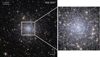 |
Fig. 2. RGB image of NGC 6397. The left-hand panel shows the entire FoV covered by the ERO data. The right-hand panel shows a 10 × 10 arcmin2 zoomed-in view of the GC core. Credits: ESA/Euclid/Euclid Consortium/NASA, image processing by J.-C. Cuillandre (CEA Paris-Saclay), G. Anselmi, CC BY-SA 3.0 IGO. |
The FoV coverage of NGC 6254 resulted in a slightly imperfect gap filling due to the dither pattern. This does not impact our scientific objective.
3. Photometric analysis
The stacked images described above were analysed using the Astromatic software suite, including Sextractor and PSFEx (Bertin 2011). Briefly, the PSFEx code models the point spread function (PSF) of an instrument as a combination of basis functions and works directly on the image. In particular, PSFEx selects point-like sources detected by Sextractor, and uses them to compute the PSF model. For both GCs investigated in this work, we selected stars for the PSF model that are bright, non-saturated, and relatively isolated in each band; specifically, we only selected point-like sources (with a maximum ellipticity of 0.3 and a FWHM within 30% of the nominal one) having at least 5 pixels above a detection threshold of 10σ above the background. A further filtering through a Moffat function has been imposed to reject spurious detections. The PSF model has been determined over a 6 × 6 equally spaced grid covering the whole FOV, allowing for a linear spatial variation. In this way, for both the GCs, the number of sources used to model the PSF exceeded a few thousand. The final PSF models have an average ellipticity of 0.02 and a FWHM spatial variation of only 3%.
These models have then been used by Sextractor to perform PSF photometry on a much larger sample of sources, defined by relaxing the source-detection threshold to having even a single pixel 1.5σ above the background. In this way, we PSF-fitted more than 400 000 sources in the VIS image of NGC 6254, and more than one million sources in the VIS image of NGC 6397. The number of detections in the NISP images is obviously lower because of reduced depth and resolution, about 190 000 for NGC 6254 and about 350 000 for NGC 6397. By combining the VIS and NISP catalogues, most of the artefacts and spurious detections (e.g. PSF spikes around very bright stars) are rejected, and the final multi-band catalogues for NGC 6254 and NGC 6397 contain positions, magnitudes, related uncertainties, and shape/quality parameters for 133 090 and 296 646 sources, respectively. Aperture corrections of a few percent (consistent with other works on ERO data; see e.g. Saifollahi et al. 2025), estimated using bright and isolated stars, are applied to the measured magnitudes. Because of the very high crowding, only a modest number of stars were fitted in the core of the clusters, where incompleteness is therefore very high. We remark, though, that throughout this paper we do not focus on the clusters’ central regions, and thus our conclusions are not affected by this. A quantitative assessment of the local completeness achieved by the ERO data of NGC 6254 in the VIS band is provided in the next section.
3.1. Completeness: Local estimate for NGC 6254
Directly estimating the completeness of the photometry would require artificial-star tests that are computationally very expensive for images this large in size, and that are not yet available in the adopted data-reduction pipeline. Nonetheless, we can take advantage of the particularly well suited, publicly available photometric catalogue by Dalessandro et al. (2011). These authors analysed HST Wide Field Planetary Camera 2 (WFPC2) observations in the F606W and F814W bands of a stellar field located between 1 and 2 rh of the cluster centre (rh = 2.02 arcmin according to Baumgardt & Vasiliev 2021). By means of artificial-star tests performed in Beccari et al. (2010), the authors computed the completeness of their WFPC2 photometric catalogue, which we can therefore use for a relative comparison.
We cross-matched our VIS catalogue with the public photometry of Dalessandro et al. (2011) by means of a linear transformation, requiring matching sources to (a) be located within a distance of 0.5 arcsec and (b) have a difference between the Euclid IE and the WFPC2 mF814W magnitudes smaller than a conservative value of 2 mag. The residuals from the resulting linear transformation solution are only 0.03 arcsec in both right ascension (RA) and declination (Dec), thus ensuring an optimally performed cross-match.
Figure 3 shows the results of the comparison. We remark that, in order to perform a meaningful analysis, we decided to exclude regions around very bright, saturated stars, which are populated by artefacts and PSF structures in both the Euclid and HST images. The red open symbols in Fig. 3 show the absolute completeness as a function of magnitude for the WFPC2 sample, as estimated by Dalessandro et al. (2011). The mF814W magnitudes were converted to IE magnitudes by means of a linear transformation depending on mF555W − mF814W colour, determined by using the stars in common between the two catalogues. On the other hand, the black filled symbols indicate the relative completeness of the VIS catalogue with respect to the WFPC2 one. As shown in the figure, the trend remains near-constant around a value of 94% down to IE = 24, and then drops to lower percentages.
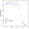 |
Fig. 3. Completeness of the Euclid ERO data in the IE band, at a distance of 1.5 rh from the core of NGC 6254. Red empty circles indicate the completeness of the reference HST/WFPC2 catalogue. Black circles represent the relative completeness of Euclid with respect to HST. Finally, the filled blue squares show the absolute completeness of the ERO VIS data. |
The product of these two curves, shown as blue filled squares in Fig. 3, provides an estimate for the absolute completeness of the VIS catalogue, at an average distance from the GC centre of 1.5 rh. This is significantly closer to the most crowded regions of the GC than the peripheries we are interested in. Moreover, this estimate does not take into account possible VIS detections that are missing in the WFPC2 catalogue. For these reasons, it is safe to consider this estimate of the catalogue completeness as a lower limit. Completeness is certainly better at larger distances in our data. As can be seen, the completeness remains about constant at ∼82% down to IE = 24, dropping to 50% completeness by IE ≃ 25.0.
The analysis of the VIS catalogue completeness has been performed to understand the ERO data better and to quantify the performance achieved, but it is not used for the study presented in this paper. These findings are of fundamental importance for future analysis of these ERO data, though, as a wealth of science cases, such as the investigation of the cluster mass functions, or of their binary populations, requires the knowledge of the photometric completeness and its correction.
3.2. Colour–magnitude diagrams
A fundamental quality check on the photometric analysis of GC fields comes from the cluster CMD. In the following, we describe the most important features we found in the CMDs of NGC 6254 and NGC 6397, which are the first Euclid CMD of Milky Way stellar systems ever presented.
3.2.1. NGC 6254
Figure 4 shows the (IE − HE, IE) CMD for an annulus between 5 and 10 arcmin from the cluster centre, as determined by Dalessandro et al. (2013a). This region has been selected as it is close enough to the cluster for the CMD to be dominated by GC stars, but far enough (well beyond 2 rh) to avoid severe incompleteness and crowding effects. The photometry has been corrected for differential reddening by using the colour excess E(B − V) map from Schlegel et al. (1998) evaluated using mwdust (Bovy et al. 2016) with the corrections from Schlafly & Finkbeiner (2011) and the extinction law by Cardelli et al. (1989). We corrected all magnitudes to a fiducial value of E(B − V) = 0.28, the mean absolute colour excess of the cluster (Harris 1996, see Fig. 5). To improve upon the correction provided by the quoted map, we further applied the differential reddening correction procedure described by Milone et al. (2012). By design, such an additional step effectively corrects also for local residuals in the photometric calibration, which can manifest as slight systematic differences in colour. Indeed, we find additional corrections of the order of a few hundredths of a magnitude, which we have applied to the observed magnitudes in Fig. 4. Overall, the CMD shows a well-defined main sequence (MS), which extends from the MSTO at IE ≈ 18.5 mag (where the deep exposures start to saturate) to a couple of magnitudes below the MS knee (see e.g. Bono et al. 2010; Massari et al. 2016; Saracino et al. 2018), located at about IE = 21.5 mag.
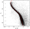 |
Fig. 4. Differential reddening-corrected (IE − HE, HE) CMD for an annulus between 300 arcsec and 600 arcsec from the centre of NGC 6254. Error bars are in grey. A 13 Gyr old, [Fe/H] = −1.5 dex and α-enhanced theoretical isochrone from the BaSTI archive is shown in red for the sake of comparison. |
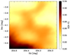 |
Fig. 5. Extinction map around NGC 6254 as obtained from the Schlafly & Finkbeiner (2011) corrections to the extinction map by Schlegel et al. (1998). |
A direct comparison with a theoretical isochrone is also shown. The isochrone has been taken from the BaSTI archive (Pietrinferni et al. 2021) and describes a 13 Gyr old population having [Fe/H] = −1.5 dex and α-enhanced ([α/Fe] = 0.4) chemical composition (Haynes et al. 2008). To take into account possible uncertainties on the absolute photometric calibration, as well as on the adopted reddening estimates (Harris 1996), the isochrone has been shifted in colour by a small arbitrary amount (δ[IE − HE] = 0.02) to provide a satisfactory fit. Once the shift is applied, the model describes the observed MS very well and shows that the observed CMD samples masses down to 0.16 M⊙ (at IE ≃ 24.9 mag). This is the deepest CMD of a GC over such a large size scale.
Another interesting feature that can be appreciated from this CMD is the possible widening of the faint MS below the MS knee. From a statistical point of view, the observed colour dispersion of upper-MS stars in the bright, non-saturated magnitude range 18.75 < IE < 19.25 mag is  mag. The typical nominal colour error at those magnitudes, as estimated by Sextractor, is of only 0.01 mag. Given that NGC 6254 is not a peculiar type-2 GC (Milone et al. 2019), and therefore should not present photometric features related to large iron or helium dispersion, which could significantly widen the observed sequences, such a nominal error seems to underestimate the actual one. We thus took the observed standard deviation
  of GC members at these bright magnitudes as a more robust (even though conservative) estimate of the photometric colour uncertainty. Possible terms that could inflate this value, making it an overestimate of the actual error, are the presence of photometric binaries, small helium variations among cluster stars, and residuals in the differential reddening correction. The observed binary fraction of NGC 6254 at the distance sampled by the CMD shown in Fig. 4 is of only 1.5% (Dalessandro et al. 2011), and therefore should not contribute significantly to
  . According to Milone et al. (2018), NGC 6254 might have a small helium spread, ΔY < 0.029, which could contribute to a photometric spread of 0.01−0.02 mag.
This colour dispersion should also increase for fainter stars due to the decrease in the signal-to-noise ratio according to  . Assuming a systematic colour uncertainty floor of
  mag at IE = 19 mag, we thus expect
  mag below the MS knee, in the range 23 < IE < 23.5 mag (see the grey error bars in Fig. 4, where the error in magnitude has been computed by assuming an equal contribution to σobs from the two bands). However, the observed colour dispersion at the same magnitudes is somewhat larger, reaching σobs = 0.12 mag. Given our conservative colour error estimate, we tentatively interpret this widening as an intrinsic feature, and cautiously attribute it to the GC’s multiple stellar populations (see e.g. Gratton et al. 2004; Milone et al. 2017), which manifest in near-IR CMDs as a widening and/or splitting of the MS below the MS-knee due to the opacity effect of collision-induced absorption by water on the surface of M-dwarfs (Milone et al. 2012, 2019). The presence of multiple-populations in NGC 6254 is widely known, both from photometric (Monelli et al. 2013; Milone et al. 2017) and spectroscopic (Carretta et al. 2009) studies. Yet, future more detailed analysis of this CMD will test the significance of this feature on more solid statistical ground, thus assessing the effectiveness of Euclid in investigating this peculiar property of GCs.
3.2.2. NGC 6397
Figure 6 shows the (IE − HE, IE) CMD for an annulus at distances r ∈ [300, 600] arcsec from the centre of NGC 6397. The CMD is corrected for differential reddening and residuals on the photometric calibration as described for NGC 6254.
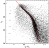 |
Fig. 6. Differential reddening-corrected (IE − HE, IE) CMD for an annulus between 300 arcsec and 600 arcsec from the centre of NGC 6397. Error bars are in grey. A 13 Gyr old, [Fe/H] = −2.0 dex, and α-enhanced theoretical isochrone from the BaSTI archive is shown in red for the sake of comparison. The effect of saturation becomes evident at IE ≲ 18.5. |
Also for NGC 6397, the cluster MS stands out very clearly as a well-defined and populated sequence, even though the contamination by field stars and background galaxies appears stronger than in the case of NGC 6254. The higher density of sources is likely the cause for the shallower depth reached by the CMD. The faintest end of the cluster MS seems to reach a magnitude of IE ∼ 24.0 mag, about 1 mag brighter than in the case of NGC 6254. Such a shallower cutoff is imposed by the limiting magnitudes in the HE band detections, which suffer from the low spatial resolution in such a crowded field and from persistence effects.
Because of the closer distance of NGC 6397 to us, saturation prevents photometric measurement of the MSTO, but we are able to sample even lower stellar masses than in the case of NGC 6254. According to the BaSTI isochrone overplotted in Fig. 6, which represents a 13 Gyr old population with [Fe/H] = −2.0 dex and α-enhanced chemical composition, the MS sampled lower limit corresponds to ∼0.12 M⊙.
The colour dispersion around the non-saturated upper MS (at IE ≲ 18.5 mag) gives once again a reasonable upper limit to the achieved photometric error of  mag, very similar to that found for NGC 6254. Following the same argument as in that cluster, the colour error below the MS knee, at 22 < IE < 22.5 mag should increase to 0.06 mag for NGC 6397 (see the error bars in Fig. 6). Again, we detect a marginal widening of the faint MS (σobs = 0.08 mag), possibly ascribable to the already known phenomenon of multiple populations in this cluster (see e.g. di Criscienzo et al. 2010; Milone et al. 2018; Carretta et al. 2009).
3.3. Star-galaxy and cluster-field separation
In order to study the morphology of the outer regions of the two GCs, it is fundamental to separate likely member GC stars from contaminating background galaxies and Milky Way disc stars. In the absence of kinematic information for all the individual sources, the best way to isolate cluster stars is to take advantage of the multi-band, high-resolution capabilities of Euclid and to combine colour information with photometric parameters that are sensitive to the point-like or extended shape of each source. Figure 7 shows the (IE − HE, IE) CMD of all sources falling in the ERO FoV around NGC 6254. When compared to the CMD shown in Fig. 4, the much higher complexity of the sampled stellar population becomes evident. In order to unravel such a complexity, we made use of two of the fit parameters provided by Sextractor, called SPREAD_MODEL and CLASS_STAR. The former parameter is designed2 such that it equals zero for stars, and deviates from zero for more extended (or more compact) sources. The latter parameter, instead, equals 1 for sources that are well fit by the adopted PSF model, and is < 1 for sources with a less satisfactory fit. Figure 8 shows the behaviour of these parameters as a function of IE magnitude. It is immediately evident that stars (yellow symbols with CLASS_STAR ∼ 1) can be rather well distinguished from other sources by imposing a selection on |SPREAD_MODEL| < 0.01. What is left out of this selection corresponds either to background galaxies (if CLASS_STAR is ≪1; see the red symbols in Fig. 7) or to saturated stars (if CLASS_STAR ∼ 1; see the blue symbols in Fig. 7).
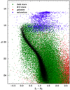 |
Fig. 7. CMD showing likely members of NGC 6254 (black), field stars (green), and background galaxies (red). |
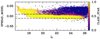 |
Fig. 8. SPREAD_MODEL as a function of IE colour-coded by CLASS_STAR. The dashed lines indicate a selection of |SPREAD_MODEL|< 0.01. |
Among what is selected as point-like sources, the stars located closer to the GC centre, and shown as black symbols in Fig. 7, describe the location of cluster members, whereas the remaining stars, shown as green symbols, represent the numerous Milky Way field stars, composed by a mix of distant halo MS stars and nearby M-dwarfs. In this case, the colour information plays the crucial role, and in particular we find that the longest colour baseline (IE − HE) is the combination of filters that best separates field stars, galaxies, and the GC stellar populations.
In summary, the CMD analysis performed in this section on NGC 6254 provides the ingredients to select likely member GC stars in the best way possible, in the absence of kinematical information. The use of the same SPREAD_MODEL and CLASS_STAR parameters, together with a colour–magnitude selection has been effective in the case of NGC 6397 as well, and is adopted hereafter, unless specifically indicated.
4. Results
4.1. Surface-brightness profiles
To build a GC surface-brightness profile that is sensitive even to very low stellar surface density, we selected a sample of likely cluster member stars by using the photometric parameters described above and by targeting completeness over purity. In this sense, we applied only conservative cuts of CLASS_STARIE > 0.03, |SPREAD_MODEL|IE < 0.01, |SPREAD_MODEL|HE < 0.01, and FLUX_RADIUSIE < 1.53, to exclude obvious artefacts and extended sources. Then, we selected our sample of GC stars along a region in the reddening-corrected CMD centred around the theoretical isochrone shown in Fig. 4, down to IE = 24 mag, and in a band ∼0.3 mag wide in IE − HE colour. As described by Fig. 7, this selection should include the vast majority of GC members.
By using these samples of selected stars, we obtain the surface-density profiles from resolved star counts for both clusters. For NGC 6254, we sub-divided the total FoV into 25 concentric annuli centred on the cluster’s centre of gravity from Dalessandro et al. (2013a), reaching a maximum cluster-centric distance r = 1400″, while we split the area sampled for NGC 6397 into 28 annuli centred on the centre reported by Goldsbury et al. (2010), thus reaching a maximum radial coverage of r = 1800″. Each annulus was then split in an adequate number of angular sub-sectors (two or four depending on the number of stars). In each sub-sector, the density has been estimated as the ratio between the selected number of stars counted and the covered area. The density assigned to a given annulus is the average of the densities of each sub-sector of that annulus. The error assigned to each density measure is defined as the dispersion around the mean of the individual sub-sector densities. We estimated the background density by using the most external data points, which attained almost constant density values. For NGC 6254 we used the six most external density values located at r > 1100″, while for NGC 6397 we could only use two data points at r > 1600″. It is worth noticing that, especially in the latter case, a few GC members are still present at these extreme radii; hence, the background density might be slightly overestimated. We then subtracted the mean background values from all the other annuli. Since the Euclid data are strongly incomplete in the inner cluster regions, we combined our resolved star count profiles with the integrated light surface brightness profiles used by Baumgardt & Hilker (2018). To this aim, we first reported our density profiles to the same scale and photometric reference systems of the literature profiles, by using values in common in the radial range 250″ < r < 400″ for NGC 6254 and 400″ < r < 650″ for NGC 6397. The resulting combined surface density profiles are shown in Figs. 9 and 10 for NGC 6254 and NGC 6397, respectively.
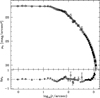 |
Fig. 9. Surface brightness profile for NGC 6254. Euclid data are shown as filled black symbols and literature values as open symbols. The solid black line marks the best-fit King model, and the grey-shaded area indicates the associated uncertainty. The bottom panel shows the residuals of the fit. |
The first key result coming from this analysis is that, while sampling almost the same radial range as previous studies, we reach surface brightness values μV ∼ 30.0 mag arcsec−2 for NGC 6254 and μV ∼ 28 mag arcsec−2 for NGC 6397, which is more than one magnitude fainter than previously obtained (e.g. Baumgardt & Hilker 2018). This performance already demonstrates the advancement that Euclid will guarantee for this kind of study in the future.
We performed a fit of the azimuthally averaged density profiles by using single-mass King models (King 1962) for both clusters, and show the results of the fit in Figs. 9 and 10. The general approach follows the one described in Dalessandro et al. (2013b). For NGC 6254 the best fit is obtained with a core radius  arcsec and a concentration parameter
  , which yields a value for the tidal radius
  arcsec. These results are in good agreement within the errors with previous estimates in the literature (e.g. Harris 1996; Dalessandro et al. 2013a). We note that rt is ∼20% larger (but still compatible within the errors) than in previous derivations. Such a large value can be naturally explained by our use of faint, low-mass MS stars, which tend to preferentially populate the cluster outer regions, while results in the literature are driven by the distribution of heavier red giant branch stars, which are generally more concentrated towards the cluster centre.
For NGC 6397, we excluded from the fit the eight innermost points (r < 12″) of the observed profile, since they appear to deviate from a flat core behavior, as expected for a post-core collapse cluster. In this way, the best-fit model is obtained for a core radius  arcsec, concentration
  and
and  arcsec. The innermost part of the profile is nicely fit with by a power law with a slope α ∼ 0.5 as typically expected for post-core collapse clusters. Because of the double fit performed in this work, results cannot be directly compared with the literature, where fits have only been performed by using a single King model.
4.2. Outer region morphology
Given the outstanding performance shown by our ERO data in terms of surface-brightness depth, we used the same sample of member stars described above to look for possible evidence of tidal tails in the two-dimensional morphology of NGC 6254 and NGC 6397. To do so, we started from NGC 6254 and computed the stellar-density map shown in Fig. 11 with over-plotted density contours at regular density intervals.
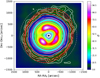 |
Fig. 11. Two-dimensional morphology of likely NGC 6254 member stars. The map is colour-coded based on the stellar density, in units of σ above the background. Iso-density contours are shown in white. The best-fitting ellipses are overplotted in red. The tidal radius as determined in this work is marked as a dashed grey circle. |
As is evident from the figure, the contours are rather circular in the inner regions but, moving outwards, they clearly develop an elongation in the north-west direction. To provide a quantitative statistical significance of the density contours plotted, we selected members stars in a region more distant than 20 arcmin from the cluster centre and computed the mean stellar density and the dispersion around the mean (σρ) in the cells of a 40 × 40 grid. The lowest-density contour shown in Fig. 11 corresponds to a density value of 5.0 σρ.
We fitted the iso-density contours with ellipses to get a quantitative idea of the morphological elongation in the cluster’s outer regions. We fixed the centres of the ellipses on (0, 0), and left the angle and the axis ratio as free parameters of the fit. The solutions of the fit are shown in Fig. 11 as red ellipses. The associated uncertainties were estimated by means of a bootstrapping algorithm, repeated 1000 times. For each iso-density contour, we discarded 50% of the sample of points used to estimate the ellipticity4, and performed the fit again. The 16th and 84th percentiles of the resulting distributions of ϵ were taken as asymmetric error estimates. The ellipticity of the iso-density contours is about zero in the inner regions and then progressively increases towards the GC peripheries, as expected in cases of tidally induced distortions, reaching a maximum of ϵ = 0.15. This trend is further described in Fig. 12, where the major-axis angles5Θ of the ellipses for the contours deviating most from circularity are represented by the tilt shown by the solid red lines, namely Θ = 60.52 deg, Θ = 61.40 deg and Θ = 51.61 deg, for a mean angle of ⟨Θ⟩ = 57.84 deg.
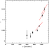 |
Fig. 12. Ellipticity of the iso-density contours as a function of distance from the centre of NGC 6254. The red lines indicate the position angle, Θ, of the best-fitting ellipse. |
When performing the same analysis on NGC 6397, we obtain the results shown in Fig. 13. The first obvious feature is that the contours appear less elongated compared to the case of NGC 6254. Also in this case they appear circular in the inner regions, and then develop a somewhat higher ellipticity towards the cluster periphery, in the north–south direction.
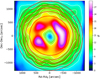 |
Fig. 13. Two-dimensional morphology of likely NGC 6397 member stars. The map is colour-coded based on the stellar density, in units of σ above the background. Iso-density contours are shown in white. The best-fitting ellipses are overplotted in red. Note that the tidal radius of NGC 6397 is outside the limits of the figure. |
The solution of the ellipsoidal fitting shown in Fig. 14 confirms the milder morphological elongation. A maximum ellipticity of ϵ = 0.07 is found in the two most external contours. The fact that we detect a weaker morphological distortion than in NGC 6254 is not surprising. The observed area for NGC 6397 covers a smaller portion of the cluster extent, as NGC 6397 is closer to the Sun and therefore appears more extended on the sky. Our observations can sample only out to about half of the cluster tidal radius of rt ∼ 0.8 deg (see Sect. 4.1). This is not likely far enough to detect distortions related to tidally induced effects. It is nonetheless reassuring that the ellipticity we find matches the one quoted by Harris (1996) and Chen & Chen (2010). The latter work also quotes a direction of the elongation (11 ± 2 deg oriented anti-clockwise from the north) that is very similar to ours. In fact, we find that the angle of the best-fit ellipses of the three most elongated density contours of our NGC 6397 map is rather stable, varying between Θ = 109.5 deg and Θ = 114.2 deg, with a mean value of Θ = 111.0 deg, corresponding to 21.0 deg in the reference system of Chen & Chen (2010).
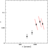 |
Fig. 14. Ellipticity of the iso-density contours as a function of distance from the centre of NGC 6397. The red lines indicate the angle of the best-fitting ellipse. |
5. Predictions from N-body simulations of NGC 6254
To understand how the morphological features observed in NGC 6254 and NGC 6397 compare with expectations, we performed an N-body simulation of each GC in the Milky Way potential. This was done using GADGET-3, which is an updated version of GADGET-2 (Springel 2005). For the Milky Way potential, we used the MWPotential2014 model from Bovy (2015), which consists of a Navarro–Frenk–White dark matter halo (Navarro et al. 1997), a Miyamoto–Nagai disc (Miyamoto & Nagai 1975) and a broken-power-law bulge. We used the present-day phase-space coordinates for NGC 6254 and NGC 6397 from Vasiliev & Baumgardt (2021). Starting from their present-day coordinates, we rewound a tracer particle for 2 Gyr to generate the initial phase-space coordinates for our models. For NGC 6254, we injected a King profile with a concentration parameter W = 7.06, a tidal radius of rt = 38.47 pc, and a mass of 1.5 × 10⁵ M⊙ (de Boer et al. 2019; McLaughlin & van der Marel 2005). We modelled this with 5 × 10⁵ equal mass particles and a particle softening of 0.0063 pc. For NGC 6397, we injected a King profile with W = 8.65, a tidal radius of rt = 32.16 pc, and a mass of 1.13 × 10⁵ M⊙ (de Boer et al. 2019; Vitral et al. 2022). We modelled this with 105 equal mass particles with a particle softening of 0.0063 pc. Both GC models were then evolved for 2 Gyr to the present day. We stress that this is an initial N-body model of both systems to study their expected tidal debris (i.e. orientation and ellipticity). As such, these models are initialised with the present-day density profiles for each GC and are disrupted for a short amount of time compared to their age (∼13 Gyr). These models are not designed to faithfully capture important effects such as two-body scattering and mass segregation. Accounting for these effects would require starting with a realistic initial mass function, using a collisional N-body code like NBODY6 (Aarseth 1999), and evolving the system for the age of the cluster, as was done in, for example, Baumgardt & Hilker (2018).
In Fig. 15 we show mock observations of our model of NGC 6254. We note that the simulated cluster is offset from the correct present-day location by 0.08 kpc in position, 3.0 km s−1 in velocity, and 0.67° in the plane of the sky from the real NGC 6254. As a result, Fig. 15 shows the coordinates relative to the centre of our simulated cluster. The star counts from the N-body simulation of NGC 6254 display a clear elongation in the north-west direction, which coincides with that found in the observations. When comparing this simulation with the iso-density contours shown in Fig. 11, their similarity is remarkable. This is highlighted even more clearly in Fig. 16, where the predicted (red triangles) and the observed (black circles) variation of NGC 6254 ellipticity as a function of the cluster radius are compared directly. In both cases, the cluster morphology remains about circular in the inner regions and then starts deviating significantly at about 13.5 arcmin. The ellipticity increases rather sharply in both the observations and the simulation by moving farther out and reaches its maximum of ϵ = 0.15 at r ∼ 18.5 arcmin. We note that in the N-body simulation, the ellipticity is estimated using the eigenvalues of the reduced moment of inertia tensor formed out of the on-sky positions of the particles in circular annuli.
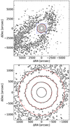 |
Fig. 15. Contour maps of an N-body simulation of NGC 6254. The top panel shows NGC 6254 over a large FOV (4 × 4 deg2). The dashed blue square shows the Euclid FOV. A dashed red circle with a radius of 1044 arcsec is included to show that the simulated cluster is tidally distorted at this radius. The contours are spaced in multiples of 10. The lower panel shows the simulation over the Euclid FoV (0.7 × 0.7 deg2). The dashed red circles are chosen to roughly match the contours to show where the cluster is expected to be tidally stretched. The circles are at radii of 225 arcsec, 468 arcsec, 738 arcsec, and 1044 arcsec. The contours are again separated by factors of 10. Note that the largest circle in the bottom panel matches the circle in the top panel. |
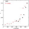 |
Fig. 16. Comparison between the radial variation in the ellipticity observed for NGC 6254 (black symbols) and the prediction from N-body simulations (red triangles). |
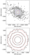 |
Fig. 17. Contour maps of an N-body simulation of NGC 6397. The top panel shows NGC 6397 over a large FoV (4 × 4 deg2). The dashed blue square shows the Euclid FOV. A dashed red circle with a radius of 1080 arcsec is included to show that the simulated cluster is not significantly tidally distorted at this radius. The contours are spaced in multiples of 10. The lower panel shows the simulation over the Euclid FOV. The dashed red circles are chosen to roughly match the contours to show where the cluster is expected to be tidally stretched. The circles are at radii of 342 arcsec, 540 arcsec, 828 arcsec, and 1080 arcsec. The contours are separated by half a dex. Note that the largest circle in the bottom panel matches the circle in the top panel. |
The consistency between the predictions from the N-body simulations strengthens significantly the interpretation of the morphological distortion we detect in the outer regions of NGC 6254 as an actual feature. This clearly indicates that NGC 6254 has experienced tidal forces due to its interaction with the Milky Way, and that these forces have distorted the cluster morphology, likely leading to the development of tidal tails on larger scales (outside the GC Jacobi radius).
In Fig. 17 we show mock observations of our model of NGC 6397. As with NGC 6254, our N-body simulation does not exactly match the present-day location and differs by 0.19 kpc, 12 km s−1, and 1.1° on the sky with observations of NGC 6397. As a result, the on-sky angles shown in Fig. 17 are relative to the centre of the simulated cluster. Our N-body simulation of NGC 6397 shows no significant tidal deformation within the Euclid FoV, but indicates that tidal deformations should be visible on larger scales. This is consistent with the fact that the Jacobi radius of NGC 6397 is larger than the FoV of Euclid.
6. Discussion and conclusions
In this paper we have analysed Euclid ERO data of two Milky Way GCs, namely NGC 6254 and NGC 6397, to investigate the presence of tidally induced morphological distortions caused by the clusters’ interaction with the Milky Way.
We have shown the first-ever Euclid CMDs of Galactic GCs. The precision in colour, ≲0.04 mag, seems to indicate the presence of a marginal colour spread in the low-mass regime, which could be associated with multiple GC populations (e.g. Milone et al. 2019), but more detailed studies are needed to confirm this. The unprecedented combination of the wide-field capability and depth further enables the detection of faint, low-mass stars down to 0.15 M⊙ and out to the GC tidal radius, at least in the case of NGC 6254. Improved understanding of the data and of the photometric analysis in the future will enable sampling of even lower stellar masses.
The surface brightness profiles built from accurately selected samples of cluster members reach more than one magnitude fainter than the surface brightness profiles presented in the literature so far for these two GCs (see e.g. Baumgardt & Hilker 2018), down to a value of μV ∼ 30.0 mag arcsec−2. Such a faint limit places them amongst the deepest ever determined, and the first to be constructed using star counts at the bottom of the MS. The tidal radius estimated from the best-fit King model of NGC 6254 is ∼20% larger than previous estimates, and such an increase can be explained by the fact that Euclid enables, for the first time, the use of low-mass MS stars, rather than giants, as morphological tracers.
Most importantly, the findings of this work provide the first robust evidence for tidally induced morphological distortions in the outer regions of NGC 6254, which implies a high chance of finding tidal tails around the cluster on the larger scales that will be covered by the Euclid survey. This evidence comes from the analysis of the two-dimensional morphology of the cluster. In fact, iso-density contours built from a sample of likely member stars reveal an elongated morphology of NGC 6254’s outer regions at more than a 5σ significance. Such an elongation is oriented along the north-west direction with a mean angle of about 58 deg, which coincides remarkably well with the direction of the cluster tidal distortions predicted by N-body simulations, and disappears towards the cluster’s inner regions. It should be noted that the direction of the elongation is somewhat reminiscent of the direction in which the extinction varies across the FoV (see Fig. 5). However, our selection of likely cluster members was performed on a differential reddening-corrected CMD, where the limiting magnitude is the one in the HE band. The colour-excess variation δE(B − V) across the field amounts to 0.15 mag corner to corner, which, based on the Cardelli et al. (1989) extinction law, corresponds to a difference in depth of only 0.08 mag in HE. We can thus safely conclude that the detected morphological distortion is not induced by differential extinction-related effects. Moreover, we have presented a remarkable similarity between the ellipticity gradient observed from the data and the one predicted by the N-body simulations. Both start from an almost circular morphology in the inner ∼10 arcmin and then rapidly increase to the maximum value of ϵ = 0.15 at a distance of ∼18.5 arcmin. This further supports the notion that the morphological elongations are indeed due to tidal features.
Finally, the two-dimensional morphology of NGC 6397 could only be sampled out to half of the GC tidal radius. It reveals a milder elongation (ϵmax = 0.07) in approximately the north–south direction, in agreement with previous studies. Further investigation on larger scales, sampling regions farther out than the cluster tidal radius (rt ≃ 0.8 deg as found in Sect. 4.1), is required to more robustly interpret this feature in terms of tidally induced morphological distortion.
To conclude, the findings of this work on Euclid ERO project demonstrate the potential that the Euclid survey has for advancing the study of star clusters in our Galaxy. To determine which GCs fall within the nominal Euclid survey coverage, we matched the 6 year Euclid wide survey region of interest (Euclid Collaboration: Scaramella et al. 2022) and planned footprint6, shown in Fig. 18, with a table of the known Milky Way GCs from Baumgardt & Hilker (2018). In total, we find that more than ∼20 Milky Way GCs will fall in the planned Euclid survey footprint. For all of these, the search for tidal tails, as well as the investigation of many other GC-related science cases, can be carried out successfully with Euclid.
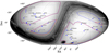 |
Fig. 18. Planned region of interest (blue polygons) and footprint (red polygons) of the full 6 year Euclid wide survey shown in a McBryde-Thomas flat polar quartic projection within blue boxes. The background represents Gaia DR3 number counts in logarithmic scale. The position and names of the GCs covered by the survey or located in its proximity are highlighted in blue. |
Data availability
Tables of the extracted photometry and positions are available at the CDS via anonymous ftp to cdsarc.cds.unistra.fr (130.79.128.5) or via https://cdsarc.cds.unistra.fr/viz-bin/cat/J/A+A/697/A8
The quoted numbers refer to the effective exposure times, whereas the total duration indicated in Euclid Collaboration: Scaramella et al. (2022) includes overheads.
We remark that the footprint currently shown in Fig. 18 could be subject to minor changes.
Acknowledgments
We are grateful to the anonymous referee for the invaluable feedback that improved the quality of the paper. DM thanks the Fundactión Jesús Serra visiting programme and the Instituto de Astrofísica de Canarias for hospitality. DM acknowledges financial support from the European Union – NextGenerationEU RRF M4C2 1.1 n: 2022HY2NSX. “CHRONOS: adjusting the clock(s) to unveil the CHRONO-chemo-dynamical Structure of the Galaxy” (PI: S. Cassisi). ED aknowledges financial support from the Fulbright Visiting Scholar program 2023. ED is also grateful for the warm hospitality of the Indiana University where part of this work was performed. AMNF acknowledges support from the UK STFC via grant ST/Y001281/1. IM acknowledges funding from UKRI/STFC through grants ST/T000414/1 and ST/X001229/1, and has received funding from the European Union’s Horizon 2020 research and innovation programme under grant agreement No. 101004214. AL acknowledges funding from Agence Nationale de la Recherche (France) under grant ANR-19-CE31-0022 This work has made use of the Early Release Observations (ERO) data from the Euclid mission of the European Space Agency (ESA), 2024, https://doi.org/10.57780/esa-qmocze3. The Euclid Consortium acknowledges the European Space Agency and a number of agencies and institutes that have supported the development of Euclid, in particular the Agenzia Spaziale Italiana, the Austrian Forschungsförderungsgesellschaft funded through BMK, the Belgian Science Policy, the Canadian Euclid Consortium, the Deutsches Zentrum für Luft-und Raumfahrt, the DTU Space and the Niels Bohr Institute in Denmark, the French Centre National d’Etudes Spatiales, the Fundação para a Ciência e a Tecnologia, the Hungarian Academy of Sciences, the Ministerio de Ciencia, Innovación y Universidades, the National Aeronautics and Space Administration, the National Astronomical Observatory of Japan, the Netherlandse Onderzoekschool Voor Astronomie, the Norwegian Space Agency, the Research Council of Finland, the Romanian Space Agency, the State Secretariat for Education, Research, and Innovation (SERI) at the Swiss Space Office (SSO), and the United Kingdom Space Agency. A complete and detailed list is available on the Euclid web site (http://www.euclid-ec.org).
References
- Aarseth, S. J. 1999, PASP, 111, 1333 [NASA ADS] [CrossRef] [Google Scholar]
- Atek, H., Gavazzi, R., Weaver, J. R., et al. 2025, A&A, 697, A15 (Euclid on Sky SI) [NASA ADS] [CrossRef] [EDP Sciences] [Google Scholar]
- Balbinot, E., & Gieles, M. 2018, MNRAS, 474, 2479 [NASA ADS] [CrossRef] [Google Scholar]
- Balbinot, E., Santiago, B. X., da Costa, L. N., Makler, M., & Maia, M. A. G. 2011, MNRAS, 416, 393 [NASA ADS] [Google Scholar]
- Baumgardt, H., & Hilker, M. 2018, MNRAS, 478, 1520 [Google Scholar]
- Baumgardt, H., & Vasiliev, E. 2021, MNRAS, 505, 5957 [NASA ADS] [CrossRef] [Google Scholar]
- Beccari, G., Pasquato, M., De Marchi, G., et al. 2010, ApJ, 713, 194 [Google Scholar]
- Belokurov, V., Evans, N. W., Irwin, M. J., Hewett, P. C., & Wilkinson, M. I. 2006, ApJ, 637, L29 [NASA ADS] [CrossRef] [Google Scholar]
- Bertin, E. 2011, ASP Conf. Ser., 442, 435 [Google Scholar]
- Bianchini, P., Ibata, R., & Famaey, B. 2019, ApJ, 887, L12 [NASA ADS] [CrossRef] [Google Scholar]
- Binney, J., & Tremaine, S. 1987, Galactic Dynamics (Princeton: Princeton University Press) [Google Scholar]
- Boldrini, P., & Vitral, E. 2021, MNRAS, 507, 1814 [NASA ADS] [CrossRef] [Google Scholar]
- Bono, G., Stetson, P. B., VandenBerg, D. A., et al. 2010, ApJ, 708, L74 [CrossRef] [Google Scholar]
- Bovy, J. 2015, ApJS, 216, 29 [NASA ADS] [CrossRef] [Google Scholar]
- Bovy, J., Rix, H.-W., Green, G. M., Schlafly, E. F., & Finkbeiner, D. P. 2016, ApJ, 818, 130 [Google Scholar]
- Carballo-Bello, J. A. 2019, MNRAS, 486, 1667 [Google Scholar]
- Cardelli, J. A., Clayton, G. C., & Mathis, J. S. 1989, ApJ, 345, 245 [Google Scholar]
- Carretta, E., Bragaglia, A., Gratton, R. G., et al. 2009, A&A, 505, 117 [NASA ADS] [CrossRef] [EDP Sciences] [Google Scholar]
- Cassisi, S., Castellani, V., degl’Innocenti, S., Salaris, M., & Weiss, A., 1999, A&AS, 134, 103 [NASA ADS] [CrossRef] [EDP Sciences] [Google Scholar]
- Chen, C. W., & Chen, W. P. 2010, ApJ, 721, 1790 [Google Scholar]
- Cuillandre, J.-C., Bertin, E., Bolzonella, M., et al. 2025a, A&A, 697, A6 (Euclid on Sky SI) [Google Scholar]
- Cuillandre, J.-C., Bolzonella, M., Boselli, A., et al. 2025b, A&A, 697, A11 (Euclid on Sky SI) [Google Scholar]
- Dalessandro, E., Lanzoni, B., Beccari, G., et al. 2011, ApJ, 743, 11 [Google Scholar]
- Dalessandro, E., Ferraro, F. R., Lanzoni, B., et al. 2013a, ApJ, 770, 45 [Google Scholar]
- Dalessandro, E., Ferraro, F. R., Massari, D., et al. 2013b, ApJ, 778, 135 [NASA ADS] [CrossRef] [Google Scholar]
- Dark Energy Survey Collaboration (Abbott, T., et al.) 2016, MNRAS, 460, 1270 [Google Scholar]
- de Boer, T. J. L., Gieles, M., Balbinot, E., et al. 2019, MNRAS, 485, 4906 [Google Scholar]
- di Criscienzo, M., D’Antona, F., & Ventura, P. 2010, A&A, 511, A70 [Google Scholar]
- Dinescu, D. I., Girard, T. M., & van Altena, W. F. 1999, AJ, 117, 1792 [Google Scholar]
- Erkal, D., Koposov, S. E., & Belokurov, V. 2017, MNRAS, 470, 60 [NASA ADS] [CrossRef] [Google Scholar]
- Euclid Collaboration (Scaramella, R., et al.) 2022, A&A, 662, A112 [NASA ADS] [CrossRef] [EDP Sciences] [Google Scholar]
- Euclid Collaboration (Schirmer, M., et al.) 2022, A&A, 662, A92 [NASA ADS] [CrossRef] [EDP Sciences] [Google Scholar]
- Euclid Collaboration (Mellier, Y., et al.) 2025, A&A, 697, A1 (Euclid on Sky SI) [Google Scholar]
- Euclid Collaboration (Cropper, M. S., et al.) 2025, A&A, 697, A2 (Euclid on Sky SI) [Google Scholar]
- Euclid Collaboration (Jahnke, K., et al.) 2025, A&A, 697, A3 (Euclid on Sky SI) [Google Scholar]
- Euclid Early Release Observations 2024, https://doi.org/10.57780/esa-qmocze3 [Google Scholar]
- Forbes, D. A., & Bridges, T. 2010, MNRAS, 404, 1203 [NASA ADS] [Google Scholar]
- Gaia Collaboration (Prusti, T., et al.) 2016, A&A, 595, A1 [NASA ADS] [CrossRef] [EDP Sciences] [Google Scholar]
- Goldsbury, R., Richer, H. B., Anderson, J., et al. 2010, AJ, 140, 1830 [NASA ADS] [CrossRef] [Google Scholar]
- Gratton, R., Sneden, C., & Carretta, E. 2004, ARA&A, 42, 385 [Google Scholar]
- Grillmair, C. J. 2019, ApJ, 884, 174 [Google Scholar]
- Grillmair, C. J., & Dionatos, O. 2006, ApJ, 643, L17 [Google Scholar]
- Grillmair, C. J., Freeman, K. C., Irwin, M., & Quinn, P. J. 1995, AJ, 109, 2553 [Google Scholar]
- Harris, W. E. 1996, AJ, 112, 1487 [Google Scholar]
- Haynes, S., Burks, G., Johnson, C. I., & Pilachowski, C. A. 2008, PASP, 120, 1097 [Google Scholar]
- Hunt, L. K., Annibali, F., Cuillandre, J.-C., et al. 2025, A&A, 697, A9 (Euclid on Sky SI) [NASA ADS] [CrossRef] [EDP Sciences] [Google Scholar]
- Hut, P., McMillan, S., Goodman, J., et al. 1992, PASP, 104, 981 [NASA ADS] [CrossRef] [Google Scholar]
- Ibata, R. A., Bellazzini, M., Malhan, K., Martin, N., & Bianchini, P. 2019, Nat. Astron., 3, 667 [Google Scholar]
- Ibata, R., Malhan, K., Martin, N., et al. 2021, ApJ, 914, 123 [NASA ADS] [CrossRef] [Google Scholar]
- Ibata, R., Malhan, K., Tenachi, W., et al. 2023, ArXiv e-prints [arXiv:2311.17202] [Google Scholar]
- Kaderali, S., Hunt, J. A. S., Webb, J. J., Price-Jones, N., & Carlberg, R. 2019, MNRAS, 484, L114 [NASA ADS] [CrossRef] [Google Scholar]
- King, I. 1962, AJ, 67, 471 [Google Scholar]
- Kluge, M., Hatch, N. A., Montes, M., et al. 2025, A&A, 697, A13 (Euclid on Sky SI) [NASA ADS] [CrossRef] [EDP Sciences] [Google Scholar]
- Kruijssen, J. M. D., Pfeffer, J. L., Chevance, M., et al. 2020, MNRAS, 498, 2472 [NASA ADS] [CrossRef] [Google Scholar]
- Kuzma, P. B., Da Costa, G. S., & Mackey, A. D. 2018, MNRAS, 473, 2881 [Google Scholar]
- Laureijs, R., Amiaux, J., Arduini, S., et al. 2011, ArXiv e-prints [arXiv:1110.3193] [Google Scholar]
- Leon, S., Meylan, G., & Combes, F. 2000, A&A, 359, 907 [NASA ADS] [Google Scholar]
- Marleau, F. R., Cuillandre, J.-C., Cantiello, M., et al. 2025, A&A, 697, A12 (Euclid on Sky SI) [NASA ADS] [CrossRef] [EDP Sciences] [Google Scholar]
- Martín, E. L., Žerjal, M., Bouy, H., et al. 2025, A&A, 697, A7 (Euclid on Sky SI) [NASA ADS] [CrossRef] [EDP Sciences] [Google Scholar]
- Massari, D., Fiorentino, G., McConnachie, A., et al. 2016, A&A, 586, A51 [NASA ADS] [CrossRef] [EDP Sciences] [Google Scholar]
- Massari, D., Koppelman, H. H., & Helmi, A. 2019, A&A, 630, L4 [NASA ADS] [CrossRef] [EDP Sciences] [Google Scholar]
- Massari, D., Aguado-Agelet, F., Monelli, M., et al. 2023, A&A, 680, A20 [NASA ADS] [CrossRef] [EDP Sciences] [Google Scholar]
- McLaughlin, D. E., & van der Marel, R. P. 2005, ApJS, 161, 304 [NASA ADS] [CrossRef] [Google Scholar]
- Meylan, G., & Heggie, D. C. 1997, A&ARv, 8, 1 [NASA ADS] [CrossRef] [Google Scholar]
- Milone, A. P., Marino, A. F., Cassisi, S., et al. 2012, ApJ, 754, L34 [NASA ADS] [CrossRef] [Google Scholar]
- Milone, A. P., Piotto, G., Renzini, A., et al. 2017, MNRAS, 464, 3636 [Google Scholar]
- Milone, A. P., Marino, A. F., Renzini, A., et al. 2018, MNRAS, 481, 5098 [NASA ADS] [CrossRef] [Google Scholar]
- Milone, A. P., Marino, A. F., Bedin, L. R., et al. 2019, MNRAS, 484, 4046 [NASA ADS] [CrossRef] [Google Scholar]
- Miyamoto, M., & Nagai, R. 1975, PASJ, 27, 533 [NASA ADS] [Google Scholar]
- Monelli, M., Milone, A. P., Stetson, P. B., et al. 2013, MNRAS, 431, 2126 [NASA ADS] [CrossRef] [Google Scholar]
- Moore, B. 1996, ApJ, 461, L13 [NASA ADS] [CrossRef] [Google Scholar]
- Moreno, E., Pichardo, B., & Velázquez, H. 2014, ApJ, 793, 110 [Google Scholar]
- Myeong, G. C., Jerjen, H., Mackey, D., & Da Costa, G. S. 2017, ApJ, 840, L25 [Google Scholar]
- Navarrete, C., Belokurov, V., & Koposov, S. E. 2017, ApJ, 841, L23 [NASA ADS] [CrossRef] [Google Scholar]
- Navarro, J. F., Frenk, C. S., & White, S. D. M. 1997, ApJ, 490, 493 [Google Scholar]
- Niederste-Ostholt, M., Belokurov, V., Evans, N. W., et al. 2010, MNRAS, 408, L66 [NASA ADS] [Google Scholar]
- Odenkirchen, M., Grebel, E. K., Rockosi, C. M., et al. 2001, ApJ, 548, L165 [Google Scholar]
- Peñarrubia, J., Varri, A. L., Breen, P. G., Ferguson, A. M. N., & Sánchez-Janssen, R. 2017, MNRAS, 471, L31 [CrossRef] [Google Scholar]
- Piatti, A. E., Mestre, M. F., Carballo-Bello, J. A., et al. 2021, A&A, 646, A176 [NASA ADS] [CrossRef] [EDP Sciences] [Google Scholar]
- Pietrinferni, A., Hidalgo, S., Cassisi, S., et al. 2021, ApJ, 908, 102 [NASA ADS] [CrossRef] [Google Scholar]
- Piotto, G., Milone, A. P., Bedin, L. R., et al. 2015, AJ, 149, 91 [Google Scholar]
- Saifollahi, T., Voggel, K., Lançon, A., et al. 2025, A&A, 697, A10 (Euclid on Sky SI) [NASA ADS] [CrossRef] [EDP Sciences] [Google Scholar]
- Salaris, M., Chieffi, A., & Straniero, O. 1993, ApJ, 414, 580 [NASA ADS] [CrossRef] [Google Scholar]
- Saracino, S., Dalessandro, E., Ferraro, F. R., et al. 2018, ApJ, 860, 95 [NASA ADS] [CrossRef] [Google Scholar]
- Sarajedini, A., Bedin, L. R., Chaboyer, B., et al. 2007, AJ, 133, 1658 [Google Scholar]
- Schlafly, E. F., & Finkbeiner, D. P. 2011, ApJ, 737, 103 [Google Scholar]
- Schlegel, D. J., Finkbeiner, D. P., & Davis, M. 1998, ApJ, 500, 525 [Google Scholar]
- Searle, L., & Zinn, R. 1978, ApJ, 225, 357 [Google Scholar]
- Shipp, N., Price-Whelan, A. M., Tavangar, K., Mateu, C., & Drlica-Wagner, A. 2020, AJ, 160, 244 [NASA ADS] [CrossRef] [Google Scholar]
- Sollima, A. 2020, MNRAS, 495, 2222 [Google Scholar]
- Sollima, A., Martínez-Delgado, D., Valls-Gabaud, D., & Peñarrubia, J. 2011, ApJ, 726, 47 [NASA ADS] [CrossRef] [Google Scholar]
- Springel, V. 2005, MNRAS, 364, 1105 [Google Scholar]
- Vasiliev, E., & Baumgardt, H. 2021, MNRAS, 505, 5978 [NASA ADS] [CrossRef] [Google Scholar]
- Vitral, E., Kremer, K., Libralato, M., Mamon, G. A., & Bellini, A. 2022, MNRAS, 514, 806 [NASA ADS] [CrossRef] [Google Scholar]
- Weaver, J. R., Taamoli, S., McPartland, C. J. R., et al. 2025, A&A, 697, A16 (Euclid on Sky SI) [NASA ADS] [CrossRef] [EDP Sciences] [Google Scholar]
- Webb, J. J., Harris, W. E., Sills, A., & Hurley, J. R. 2013, ApJ, 764, 124 [Google Scholar]
- York, D. G., Adelman, J., Anderson, J. E., et al. 2000, AJ, 120, 1579 [Google Scholar]
All Figures
|
Fig. 1. Sky coverage and dither pattern of the four VIS (left-hand panel) and NISP (right-hand panel) exposures of the ERO ROS for NGC 6254. Red symbols indicate Gaia reference stars. Green symbols represent Euclid detections. |
| In the text | |
|
Fig. 2. RGB image of NGC 6397. The left-hand panel shows the entire FoV covered by the ERO data. The right-hand panel shows a 10 × 10 arcmin2 zoomed-in view of the GC core. Credits: ESA/Euclid/Euclid Consortium/NASA, image processing by J.-C. Cuillandre (CEA Paris-Saclay), G. Anselmi, CC BY-SA 3.0 IGO. |
| In the text | |
|
Fig. 3. Completeness of the Euclid ERO data in the IE band, at a distance of 1.5 rh from the core of NGC 6254. Red empty circles indicate the completeness of the reference HST/WFPC2 catalogue. Black circles represent the relative completeness of Euclid with respect to HST. Finally, the filled blue squares show the absolute completeness of the ERO VIS data. |
| In the text | |
|
Fig. 4. Differential reddening-corrected (IE − HE, HE) CMD for an annulus between 300 arcsec and 600 arcsec from the centre of NGC 6254. Error bars are in grey. A 13 Gyr old, [Fe/H] = −1.5 dex and α-enhanced theoretical isochrone from the BaSTI archive is shown in red for the sake of comparison. |
| In the text | |
|
Fig. 5. Extinction map around NGC 6254 as obtained from the Schlafly & Finkbeiner (2011) corrections to the extinction map by Schlegel et al. (1998). |
| In the text | |
|
Fig. 6. Differential reddening-corrected (IE − HE, IE) CMD for an annulus between 300 arcsec and 600 arcsec from the centre of NGC 6397. Error bars are in grey. A 13 Gyr old, [Fe/H] = −2.0 dex, and α-enhanced theoretical isochrone from the BaSTI archive is shown in red for the sake of comparison. The effect of saturation becomes evident at IE ≲ 18.5. |
| In the text | |
|
Fig. 7. CMD showing likely members of NGC 6254 (black), field stars (green), and background galaxies (red). |
| In the text | |
|
Fig. 8. SPREAD_MODEL as a function of IE colour-coded by CLASS_STAR. The dashed lines indicate a selection of |SPREAD_MODEL|< 0.01. |
| In the text | |
|
Fig. 9. Surface brightness profile for NGC 6254. Euclid data are shown as filled black symbols and literature values as open symbols. The solid black line marks the best-fit King model, and the grey-shaded area indicates the associated uncertainty. The bottom panel shows the residuals of the fit. |
| In the text | |
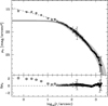 |
Fig. 10. Same as Fig. 9 but for NGC 6397. |
| In the text | |
|
Fig. 11. Two-dimensional morphology of likely NGC 6254 member stars. The map is colour-coded based on the stellar density, in units of σ above the background. Iso-density contours are shown in white. The best-fitting ellipses are overplotted in red. The tidal radius as determined in this work is marked as a dashed grey circle. |
| In the text | |
|
Fig. 12. Ellipticity of the iso-density contours as a function of distance from the centre of NGC 6254. The red lines indicate the position angle, Θ, of the best-fitting ellipse. |
| In the text | |
|
Fig. 13. Two-dimensional morphology of likely NGC 6397 member stars. The map is colour-coded based on the stellar density, in units of σ above the background. Iso-density contours are shown in white. The best-fitting ellipses are overplotted in red. Note that the tidal radius of NGC 6397 is outside the limits of the figure. |
| In the text | |
|
Fig. 14. Ellipticity of the iso-density contours as a function of distance from the centre of NGC 6397. The red lines indicate the angle of the best-fitting ellipse. |
| In the text | |
|
Fig. 15. Contour maps of an N-body simulation of NGC 6254. The top panel shows NGC 6254 over a large FOV (4 × 4 deg2). The dashed blue square shows the Euclid FOV. A dashed red circle with a radius of 1044 arcsec is included to show that the simulated cluster is tidally distorted at this radius. The contours are spaced in multiples of 10. The lower panel shows the simulation over the Euclid FoV (0.7 × 0.7 deg2). The dashed red circles are chosen to roughly match the contours to show where the cluster is expected to be tidally stretched. The circles are at radii of 225 arcsec, 468 arcsec, 738 arcsec, and 1044 arcsec. The contours are again separated by factors of 10. Note that the largest circle in the bottom panel matches the circle in the top panel. |
| In the text | |
|
Fig. 16. Comparison between the radial variation in the ellipticity observed for NGC 6254 (black symbols) and the prediction from N-body simulations (red triangles). |
| In the text | |
|
Fig. 17. Contour maps of an N-body simulation of NGC 6397. The top panel shows NGC 6397 over a large FoV (4 × 4 deg2). The dashed blue square shows the Euclid FOV. A dashed red circle with a radius of 1080 arcsec is included to show that the simulated cluster is not significantly tidally distorted at this radius. The contours are spaced in multiples of 10. The lower panel shows the simulation over the Euclid FOV. The dashed red circles are chosen to roughly match the contours to show where the cluster is expected to be tidally stretched. The circles are at radii of 342 arcsec, 540 arcsec, 828 arcsec, and 1080 arcsec. The contours are separated by half a dex. Note that the largest circle in the bottom panel matches the circle in the top panel. |
| In the text | |
|
Fig. 18. Planned region of interest (blue polygons) and footprint (red polygons) of the full 6 year Euclid wide survey shown in a McBryde-Thomas flat polar quartic projection within blue boxes. The background represents Gaia DR3 number counts in logarithmic scale. The position and names of the GCs covered by the survey or located in its proximity are highlighted in blue. |
| In the text | |
Current usage metrics show cumulative count of Article Views (full-text article views including HTML views, PDF and ePub downloads, according to the available data) and Abstracts Views on Vision4Press platform.
Data correspond to usage on the plateform after 2015. The current usage metrics is available 48-96 hours after online publication and is updated daily on week days.
Initial download of the metrics may take a while.