| Issue |
A&A
Volume 696, April 2025
|
|
|---|---|---|
| Article Number | A84 | |
| Number of page(s) | 11 | |
| Section | Stellar structure and evolution | |
| DOI | https://doi.org/10.1051/0004-6361/202453493 | |
| Published online | 07 April 2025 | |
Another one (BH+OB pair) bites the dust
Groupe d’Astrophysique des Hautes Energies, STAR, Université de Liège, Quartier Agora (B5c, Institut d’Astrophysique et de Géophysique), Allée du 6 Août 19c, B-4000 Sart Tilman, Liège, Belgium
⋆ Corresponding author; This email address is being protected from spambots. You need JavaScript enabled to view it.
Received:
18
December
2024
Accepted:
25
February
2025
Abstract
Aims. Most (or possibly all) massive stars reside in multiple systems. From stellar evolution models, numerous systems with an OB star coupled to a black hole would be expected to exist. There have been several claimed detections of such pairs in recent years and this is notably the case of HD 96670.
Methods. Using high-quality photometry and spectroscopy in the optical range, we revisited the HD 96670 system. We also examined complementary X-ray observations to provide a broader view of the system properties.
Results. The TESS light curves of HD 96670 clearly show eclipses, ruling out the black hole companion scenario. This does not mean that the system is not of interest. Indeed, the combined analysis of photometric and spectroscopic data indicates that the system most likely consists of a O8.5 giant star paired with a stripped-star companion with a mass of ∼4.5 M⊙, a radius of ∼1 R⊙, and a surface temperature of ∼50 kK. While several B+sdOB systems have been reported in the literature, this would be the first case of a Galactic system composed of an O star and a faint stripped star. In addition, the system appears brighter and harder than normal OB stars in the X-ray range, albeit less so than for X-ray binaries. The high-energy observations provide hints of phase-locked variations, as typically seen in colliding wind systems. As a post-interaction system, HD 96670 actually represents a key case for probing binary evolution, even if it is not ultimately found to host a black hole.
Key words: binaries: close / binaries: eclipsing / binaries: spectroscopic / stars: black holes / stars: massive / subdwarfs
F.R.S.-FNRS Senior Research Associate.
© The Authors 2025
 Open Access article, published by EDP Sciences, under the terms of the Creative Commons Attribution License (https://creativecommons.org/licenses/by/4.0), which permits unrestricted use, distribution, and reproduction in any medium, provided the original work is properly cited.
This article is published in open access under the Subscribe to Open model. This email address is being protected from spambots. You need JavaScript enabled to view it. to support open access publication.
1. Introduction
At the end of their eventful lives, it is commonly believed that the most massive objects of the stellar population (∼20 − 150 M⊙) give rise to stellar-mass black holes (BHs). Following population synthesis models, the Milky Way alone would be expected to harbour thousands, if not millions, of BHs (e.g. Lamberts et al. 2018; Olejak et al. 2020). Furthermore, since most (if not all) massive stars lie in multiple systems, it should not be surprising to find many cases of BHs paired with an OB star or double BH systems. In fact, such detections would prove invaluable for constraining stellar evolution models, especially with respect to binary interactions. However, while double compact systems are now regularly detected during mergers, based on their gravitational wave emissions, identifying BH+OB systems has proven to be elusive despite intense observational efforts.
In binary systems composed of a compact object and a massive star, the former object can accrete material either from the wind of the massive star or following a Roche lobe overflow of that star, leading to copious X-ray emissions. Over a hundred such systems, called high-mass X-ray binaries, are currently known in our Galaxy (Fortin et al. 2023). However, amongst them, only Cyg X-1 appears to be a secure and undisputed case involving a BH (Miller-Jones et al. 2021). In parallel, since some BH+OB pairs might be X-ray quiet, several recent searches have instead used optical spectroscopy to perform in-depth investigations of massive SB1 systems (e.g. Mahy et al. 2022). Several proposals for BH+OB candidates followed, but most detection claims were soon disproved; for instance, LB-1 (El-Badry & Quataert 2020), HR 6819 (Gies & Wang 2020; Bodensteiner et al. 2020), MWC 656 (Rivinius et al. 2024), NGC 1850 BH1 (El-Badry & Burdge 2022a), or NGC 2004 #115 (El-Badry et al. 2022b). In this paper, we propose to take a new look at such a BH+OB candidate, HD 96670.
HD 96670 is a hot star of the Carina OB2 association, classified by Sota et al. (2014) as O8.5(n)fp var (the ‘var’ suffix added because of varying He IIλ4686 Å). In fact, HD 96670 was already noted as variable by Conti et al. (1977) and reported to be a short-period (5 d) binary by Garcia (1994), who proposed the first orbital solution. Since only one component was seen in the spectra, only an SB1 solution could be derived. Adding two velocity points from IUE, but discarding low-resolution data from Thackeray et al. (1973), Stickland & Lloyd (2001) refined the orbital solution. Using interferometry, Sana et al. (2014) found a third star in the system, with ΔH ∼ 1.26 mag and d ∼ 30 mas. Lastly, Gomez & Grindlay (2021) reported photometric variations in addition to the velocity modulation. They interpreted them as ellipsoidal variations (plus a flare). They also found asymmetries in He I and O lines (photospheric He II lines appearing unaffected) as well as a shift between their velocities and those used by Stickland & Lloyd (2001), both of which they consider as the signature of the third star (the first one being a direct signature, while the second is an indirect signature as it would be the reflex motion due to that third star). They calculated orbital solutions using photometric and spectroscopic variations separately, but they also combined both pieces of information to get a global solution. In both cases, they found that the companion should have a mass of about 6 M⊙, although no trace of it was detected in the optical spectra. This absence of optical signature, combined with the detection of hard X-rays with NuSTAR, led them to conclude that HD 96670 most probably contains a BH companion.
To revisit the properties of HD 96670, we use optical and X-ray data, first presented in Sect. 2 and then analysed in Sect. 3. These observational constraints lead to a re-assessment of the system’s nature, which is discussed in Sect. 4.
2. Data
2.1. Stellar properties
In the Gaia-DR3 catalog (Bailer-Jones et al. 2021), HD 96670 displays a distance of  pc. The Gaia parallax appears secure (small error as Rplx = π/σπ = 11.1 and good quality as RUWE = 1.2). This is in line with other determinations (Garcia 1994), but Gomez & Grindlay (2021) nevertheless preferred to use the distance from a set of neighbouring Carina stars (2.83 kpc). In Simbad, HD 96670 appears with magnitudes B = 7.60 and V = 7.43. Its reddening has been evaluated to E(B − V) = 0.39 mag by Bowen et al. (2008) and 0.43 mag by Savage et al. (2001) or from the B − V and the calibration of Martins & Plez (2006) for O8.5 stars. This leads to absolute magnitudes of MV = −6.04 for the lowest extinction and distance and MV = −6.48 for the largest ones. Martins et al. (2005) listed MV values of −4.19, −5.32, and −6.29 for O8.5 V, III, I stars, respectively. On this basis alone, HD 96670 would thus be classified as a supergiant and this luminosity class sometimes appears in the literature (Savage et al. 2001; Sana et al. 2014). Using the bolometric correction for supergiants, we would then derive a bolometric luminosity of log(LBOL/L⊙) = 5.47 − 5.65 for HD 96670; it would be 5.51–5.69 when adopting the bolometric correction for giants.
2.2. TESS
HD 96670 was observed over five months by the TESS satellite (Ricker et al. 2015), in Sectors 10, 11, 37, 63, and 64. Sky images were taken with a cadence of 30 min in the first two Sectors, 10 min for Sectors 37, and 200 s for the last two Sectors. The sector duration leads to a natural peak width in frequency space of 1/25 d; namely, 0.04 d−1. The TESS data were reduced and calibrated using a pipeline inspired by that of the Kepler mission. Individual light curves were then derived from image cutouts of 51 × 51 pixels using aperture photometry performed with the Python package Lightkurve1. The source mask was defined from pixels with fluxes above 30 times the Median Absolute Deviation over the median flux, while the background mask was defined by pixels with fluxes below the median flux (i.e. below the null threshold). To estimate the background, two methods were used: (1) a principal component analysis (PCA), with five components; (2) a simple median calculation. In each case, the two background-subtracted light curves were compared. The PCA-corrected light curves were similar or better (less long-term trends) and they were thus retained. The TESS fluxes were converted into magnitudes and the average magnitude was subtracted from each individual light curve.
Since TESS has a rather coarse PSF, we examined the environment of HD 96670 in Gaia-DR3. Within a one arcmin radius (about 3 TESS pixels, typical of the chosen apertures), all other objects display magnitude differences of Δ(G) > 4 mag. The ten brightest neighbours have Δ(G) = 4 − 8 mag, with separations of 0.5–1′. Thus, only scarce contamination is expected from these stars.
2.3. FEROS
The high-resolution echelle spectrograph FEROS, installed on the 2.2 m telescope at La Silla observatory (European Southern Observatory, ESO), was used to observe HD 96670 nine times. Eight spectra, taken between 2004 and 2009 (Obs ID 074.D-0300, 076C-0431, 076D-0294, and 083.D-0589), are publicly available and were downloaded from the ESO archives2. Their signal-to-noise ratios (S/Ns) lie between 170 and 350. We note that the heliocentric correction was directly applied to these spectra. The spectra were normalized in several regions harbouring the main photospheric lines (4000–4600, 4600–5100, 5350–5950, and 6400–6700 Å).
2.4. X-ray data
The Chandra X-ray telescope observed HD 96670 slightly off-axis in October 2020 (ObsID 23643). Its spectrum was built using CIAO v4.16. The X-ray data were extracted around the Simbad coordinates of HD 96670 in a circle of 10 pixels radius and the background was taken in the surrounding annulus with an outer radius of 30 pixels. A minimum number of counts of 10 was used to bin the spectrum and weighted spectral matrices were built during data extraction using the SPECEXTRACT task.
The Swift X-ray telescope observed HD 96670 in PC mode nine times. The light curve was built using the on-line tool3 in the 0.5–10. keV band. The number of collected counts is low so no individual spectroscopic analysis can be performed and only a combined spectrum was built using the same tool, then the same grouping as for Chandra was applied. These Swift data must be taken with caution. Indeed, the X-ray measurements suffer from optical contamination if the targets are optically bright: the limit for hot stars is around V = 8.4, while HD 96670 has V = 7.4. One may note that the photometric changes (of a few mmag) are too small to significantly affect this contamination. This being said, we stress that the combined Swift spectrum shows no strong excess at very low energies, as is typically recorded in case of optical loading. Therefore, we decided to (cautiously) examine the Swift data. Extraction was however performed considering all grades but also keeping only grade = 0, since this yields more reliable data and guarantees the absence of optical contamination (although it lowers the S/N).
3. The HD 96670 system
3.1. Constraints from velocities
In the FEROS spectra (Fig. 1), the profiles of some spectral lines show no morphological changes but display changing Doppler shifts, such as He II absorption lines, which were known to be unaffected by contamination (Gomez & Grindlay 2021). In contrast, these authors found Balmer and He I lines to be contaminated by the third star and we confirm here their asymmetric appearance, at some phases. Finally, some lines display a complex behaviour. This is notably the case of Hα or He IIλ4686 Å (Fig. 1). The profile of these lines is a combination of emission and absorption. In the spectra of Gomez & Grindlay (2021, see their Figure 8), the He II emission always appeared at ∼200 km s−1, on the red-shifted side. These authors interpreted it as ‘a complex accretion wind’. In some of our profiles as well as in those shown by Sota et al. (2014, see their Figure 7), emission appears on both the red-shifted and the blue-shifted sides. Thus, the line profile is far from constant, with complex variations.
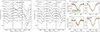 |
Fig. 1. Left and middle panels: various lines recorded in the eight FEROS spectra, with arbitrary vertical shifts to make differences clearer (oldest spectrum on top, earliest at bottom). Right: lines corrected for the average He II velocity (Table 1): He II and C IV display no profile change, while H and He I do. |
The radial velocities (RVs) were measured by fitting Gaussians to the bottom part of the photospheric He II lines at 4199.83, 4541.59, and 5411.53 Å. For completeness, we also measured the velocities of two Balmer lines in the same way (Hγλ4340.468 Å and Hβλ4861.33Å), three He I lines (at 4026.072, 4471.512, 5875.62 Å), and several metallic lines (Si IVλ4088.863 Å, N IIIλ4379.09,4634.25 Å, O IIIλ5592.252 Å, and C IVλ5801.34,5811.97 Å, which are all in absorption, except N IIIλ4634). The velocities from photospheric lines of He II and metals are in excellent agreement, but differences are sometimes detected with the other lines (Fig. 2). Table 1 provides average velocities from lines of H, He I, He II, and metals (only absorptions). As they appear the most secure, RVs from photospheric He II lines will be considered as our reference velocities, as done by Gomez & Grindlay (2021). A period search algorithm (Heck et al. 1985; Gosset et al. 2001) was applied to the full RVs set, namely, by complementing data from Conti et al. (1977), Garcia (1993), Stickland & Lloyd (2001), and Gomez & Grindlay (2021) with our own. The best frequency was found at 0.189255 ± 0.000005 d−1, corresponding to a period of 5.28388 ± 0.00018 d in line with that of Gomez & Grindlay (P = 5.28388 ± 0.00046 d).
RVs of HD 96670.
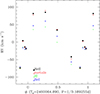 |
Fig. 2. RVs measured on FEROS data from different sets of lines. |
In each study, different sets of lines are used, so that shifts between them may occur. In addition, the presence of a third body could also lead to velocity shifts from epoch to epoch. Gomez & Grindlay (2021) reported a shift of 16.7 km s−1 between their data (spread over a year) and those of previous studies (spread over 4000 d). Our FEROS velocities (spread over 1600 d) also display such shifts, as can be seen in the left panel of Figure 3. In this figure, phase zero corresponds to the deeper eclipse (see Sect. 3.2), namely, to a conjunction. The orbital solution of Stickland & Lloyd (2001), also shown on the figure, has a T0 corresponding to periastron and, from the orbital solution, we can calculate that the conjunction occurs at ϕc = 0.097. Thus, we shifted the Stickland & Lloyd solution RV curve by −0.097 to display it on Fig. 3.
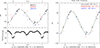 |
Fig. 3. Left: RVs of HD 96670 used by Stickland & Lloyd (2001: black dots), averages of the RVs derived by Gomez & Grindlay (2021: blue triangles), and RVs measured on FEROS data (red stars). The Stickland & Lloyd solution is also shown – beware that the period used by these authors was different. The bottom panel displays the average TESS LC, phased with the same ephemeris. Right: shifted RVs along with the solutions of Stickland & Lloyd (black line, with γ set to zero) and ours (dotted green line). Here, ϕ = 0 corresponds to conjunction with the O star in front and only the FEROS points from 2006 (marked with an asterisk in Table 1) are shown. |
We further used the Stickland & Lloyd solution to calculate the expected RVs for the phase of each spectroscopic observation, calculated from our period and T0, plus considering the above phase shift. The observed minus predicted RV residuals do not show any coherent trend with time, as would be expected for reflex motion due to the presence of a third body (Fig. 4). However, we should not exclude the possibility that the noise is hiding small orbital variations. Clearly, a long-term, high quality monitoring of HD 96670 is needed to assess whether reflex motion is present and (if it is) to constrain the orbit around the third body.
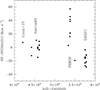 |
Fig. 4. Difference between RVs of HD 96670 and the solution of Stickland & Lloyd (2001). |
We then considered observing sets taken within a year (see * in Table 1); namely, we discarded isolated data points and calculated the average differences in each yearly set. We found average shifts RV − RVS & L of −1.1, 36.6, and −17.4 km s−1 for neighbouring velocities of Garcia (1993), from FEROS data of 2006, and for RVs of Gomez & Grindlay (2021), respectively. These RVs were corrected for these shifts and also for the γ = −9 km s−1 of the Stickland & Lloyd solution. The Liège orbital solution package (LOSP4) was then used to derive the best orbital solution. It is provided in Table 2 and shown on the right panel of Fig. 3. The rms is 10 km s−1, and the agreement with the Stickland & Lloyd solution is excellent. The mass function implies that for a primary of 33.9 M⊙, the typical mass of an O8.5I star (Martins et al. 2005), the secondary would have 5.4–5.8 M⊙ for inclinations of 90–70°. This corresponds to mass ratios of q = M2/M1 = 0.16 − 0.17.
Orbital solution for HD 96670.
Gomez & Grindlay (2021) do not list T0 (whether periastron or conjunction), K, nor f(m), prohibiting comparison. They do provide eccentricity and periastron argument but the parameters strongly depend on the chosen model. In their Model 1, these authors fitted the photometry and spectroscopy together, leading to e = 0.28 ± 0.01 and ω = 0.79 ± 0.03 rad (i.e. 45.3 ± 1.7°). In their Model 2, they fitted periastron argument separately for photometry and spectroscopy and derived e = 0.12 ± 0.01 with ωRV = 1.10 ± 0.06 rad (i.e. 63.0 ± 3.4°) and ωphot = 5.91 ± 0.06 rad (i.e. 338.6 ± 3.4°). The large eccentricity variation is not discussed but these authors attributed the large difference in the periastron argument to tidal effects. However, their photometric and spectroscopic datasets were taken in June 2015–April 2016 and April 2016–February 2017, respectively. The average difference between datasets thus is one year, but their individual duration is also of about one year. If apsidal motion was that large, namely, 1.5 rad (or 85°) over a year, the spectroscopic and photometric datasets should not be combined; at the same time, neither the photometric dataset nor the spectroscopic one should be analysed as a single entity. Indeed, between the start and the end of each dataset, ω would have changed so much that the analysis should include the ω variations, which was not done. However, (1) apsidal motion in massive binaries usually appears much less extreme (examples of large values are 7.5° yr−1 in Y Cyg, Harmanec et al. 2014, and 15° yr−1 in CPD–41°7742, Rosu et al. 2022) and (2) high-quality light curves do not confirm the photometric interpretation of Gomez & Grindlay (2021). More details are given in the next subsection.
Finally, a last note ought to be made on the FEROS spectra. While the relative strength of the He I and He II lines confirms the O8.5 type, the spectra also display a Si IVλ4088 Å line similar in intensity to the nearby He Iλ4143 Å. For late O-type stars, this suggests a main sequence classification, a luminosity class also adopted by Garcia (1993). A more general comparison with the atlas of Sota et al. (2011) also favour a main sequence class. However, the absolute magnitude MV (derived in previous subsection) is 2 mag too bright for a main sequence classification and the presence of faint companions (see Sana et al. 2014 and the next subsection) are not sufficient to explain such a large difference.
To search for spectral signatures of the secondary star, we used our implementation of the shift-and-add spectral disentangling method described by González & Levato (2006). Spectral disentangling takes advantage of the Doppler shifts at different orbital phases to iteratively reconstruct the individual mean spectra of the components of a binary system. The González & Levato (2006) method allows us (in principle) to simultaneously determine the individual RVs for each epoch of observation (see e.g. Rauw & Nazé 2016). However, in the present case, we fixed the RVs of the primary star to those determined for He II (see Table 1). The RVs of the secondary were computed from our best estimate of the mass ratio q = 0.18 (see next subsection), considering the zero point of −27.6 km s−1 mentioned above, and were also kept fixed in the disentangling process, as done in Nazé et al. (2023). This method was applied to data over the spectral ranges from 4000–5080 Å and 6430–6730 Å. We used 200 iterations, allowing to remove any residuals from the initial approximation of flat, featureless spectra. To avoid any shift in the systemic velocity that could arise on longer timescales because of the presence of a third component, we restricted ourselves to the six FEROS spectra that were taken within two months in 2006. The results are displayed in Fig. 5.
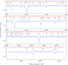 |
Fig. 5. Results of the disentangling applied to the six FEROS spectra from 2006, keeping the RVs fixed and assuming q = 0.18. The reconstructed spectra of the primary (blue) and secondary (red) are normalized against the combined continuum of the system. For clarity, the normalized secondary spectrum is shifted vertically by 0.2. |
We stress that the disentangled spectra, especially that of the primary, could suffer from contamination of the tertiary spectrum. We attempted to disentangle the spectra accounting for three components, but these attempts were not successful. Indeed, the RV amplitude of the primary is rather low, leading to severe cross-contamination of the primary and tertiary spectral components. We thus restricted ourselves to the disentangling of two spectral signatures (i.e. the primary and the secondary spectra). With those caveats in mind, we find that the reconstructed primary spectrum appears very much as we would expect for a late O-type star. Some remarkable features are the N IIIλ4634-4640 emissions, along with a double-peaked He IIλ 4686 emission. These features qualify the primary as an Of star and the double-peaked morphology of He IIλ 4686 even suggests an Onfp/Oef classification. However, the objects of the latter category are usually of earlier spectral types and are faster rotators (Rauw & Nazé 2021) than the primary of HD 96670. Indeed, we used the Fourier method to establish the projected rotational velocity v sin i of the primary (Simón-Díaz & Herrero 2007). For this purpose, we used the C IIλ 4268, the O IIλ 4276 and the Si IIIλ 4568 lines on the primary disentangled spectrum. We obtained a value of v sin(i) = (175 ± 3) km s−1, which falls in between published values (135 km s−1 in Stickland & Lloyd 2001 and ∼200 km s−1 in Gomez & Grindlay 2021).
The reconstructed secondary spectra unveil only a limited number of lines. All H I Balmer lines display relatively broad and shallow absorptions. Broad absorptions, possibly with an emission reversal in the core, are also seen in the strongest He I lines (at 4026, 4471, 4921 Å), whereas, with the exception of He IIλ 4686, He II lines are absent from the secondary spectrum. Hα exhibits a similar profile to the He I lines possibly flanked by two broad emission features. Whilst these results must be considered as preliminary, we note that the spectral reconstructions are quite insensitive to q. Indeed, we tested mass-ratios between 0.16 and 0.20 and the reconstructed spectra were essentially identical.
We may, however, note some limitations of this disentangling trial. First, only six spectra could be used, which of course limits the quality of the result: disentangling should be re-tried with a much more intense monitoring (with also an increased S/N and redundancy). Second, there is an intrinsic limitation to the reconstruction. Indeed, the lines dominating the spectrum come from the primary spectrum and they are broader than its orbital motion (i.e. v sin(i) > K). The contribution of the secondary and tertiary stars most probably ends up partially confused with the primary contribution. This impairs the disentangling, which works best on well-separated signatures.
Finally, we took a second look at the two IUE spectra5 used by Stickland & Lloyd (2001). After normalization, the IUE spectra were cross-correlated, considering wavelength ranges avoiding strong wind lines (e.g. C IV near 1550 Å), against a TLUSTY OSTAR2002 spectrum (Lanz & Hubeny 2003) with high temperature and high log(g), as in Wang et al. (2021). While we could retrieve the peak in the cross-correlation function corresponding to the primary star, no specific feature was detected at the expected velocity of the secondary star. This non-detection is not totally surprising as the S/N of these IUE spectra was low and the temperature contrast between both components is lower than for Be+subdwarf systems, which makes detection more complex (Jones et al. 2022).
3.2. Constraints from the light curves
The TESS light curves are shown on the left side of Fig. 6. Regular deeper dips of about 20 mmag are readily detected, with a separation of about 5 days (i.e. similar to the orbital period). There are, however, additional oscillations (notably, additional dips in between the main ones). The deeper dips and the intermediate ones clearly represent primary and secondary eclipses. In other words, this behaviour does not resemble the ellipsoidal variations (45 mmag peak-to-peak) along with a flare of a similar amplitude described by Gomez & Grindlay (2021). In fact, their ground-based data can be retrieved from the paper publisher website as well as at CDS6: it appears that they clearly suffered from a huge scatter, which explains the difficulty to interpret them (see more details below).
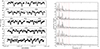 |
Fig. 6. TESS light curves of HD 96670, and their associated periodograms. Dotted red lines in the right panels indicate the orbital frequency and its harmonics. |
Frequency spectra were calculated for each Sector data using the same modified Fourier algorithm as in previous subsection (Heck et al. 1985; Gosset et al. 2001). The frequency spectra clearly show peaks at the orbital frequency and its harmonics (see right panels of Fig. 6). The strongest peak corresponds to the first harmonics at 0.376 ± 0.004 d−1. There is no strong peak in addition to these harmonics. Therefore, no evidence for additional rotational modulation or pulsational activity has been found, but there clearly is red noise, as is common in massive stars (Bowman et al. 2020; Nazé et al. 2021).
The light curves of Sectors 10+11, 37, and 63+64 were folded using T0 = 2460064.890 and an orbital frequency of 0.18925 d−1 which provides the best phasing of the deepest eclipses. This frequency is only slightly lower than that derived from spectroscopy (0.189255 d−1) and compatible with it, within the errors. These folded curves were then binned to get average phased light curves with 100 phase bins (left panel of Fig. 7). In the binned light curves, the stochastic ‘noise’ is much lower; hence, the second eclipse is much more obvious. The main eclipses are well centered on ϕ = 0, but the phasing may seem less good for the second eclipses (see insets of left panel of Fig. 7). When the orbital frequency derived from the spectroscopy (0.189255 d−1) is used instead, the results appear very similar, although the second eclipses agree well, while slight shifts are seen for main eclipses (see right panel of Fig. 7 and its insets). These shifts are very small, Δ(ϕ) = 0.01, but might be due to slow apsidal motion. However, they may also have a more mundane explanation. Indeed, the depth of the eclipses changes by about 2 mmag in these average curves and additional dips also appear in between the eclipses. Furthermore, the typical dispersions around the average amount to ∼5 mmag (Fig. 7). The orbital signal is thus nearly of the same order of magnitude as the additional variations (Fig. 6), which may blur the eclipse profiles, giving an appearance of shifts. We therefore decided to use the spectroscopic orbital period for the light curve analysis.
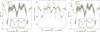 |
Fig. 7. Binned light curves for the three TESS observing campaigns (left) and for the Gomez & Grindlay photometry (middle, a zero point of 7.62 was subtracted) using forb = 0.189250 d−1. Error bars correspond to a 1σ dispersion in each bin. Right: Same as left panel but using forb = 0.189255 d−1 (the spectroscopic one). |
We also binned the Gomez & Grindlay BVR data. Due to the coarser coverage of the orbital cycle, only 20 bins were used here. No distinction was made between the different filters as the filter information is missing in the available data. In addition, in Gomez & Grindlay (2021), all BVR data were considered together so the same approach was followed here. The middle panel of Fig. 7 compares these binned curves to the average TESS curves. Whatever the chosen orbital frequency, they appear fully compatible with each other. In particular, the eclipses are also present in the ground-based data, although the data display a huge dispersion: it is most likely that the low precision is what led to the previous erroneous interpretation.
In Figure 3, the folding is done using the photometric T0 and the spectroscopic P. It may be noted that the main eclipse occurs when the RV of the primary star increases, namely, at the conjunction with the O star primary in front of its companion. Furthermore, the flat bottom of the eclipses suggest that the companion is fully eclipsed. Therefore, the fact that this deepest eclipse occurs when the O star occults its companion implies that this companion is hotter than the primary star. As we show below, this conclusion is confirmed by fitting the light curves with a binary model.
To analyse the photometry, we built an overall mean light curve to help to get rid (as much as possible) of the stochastic variations and better isolate the orbital signal. To this aim, we did not consider the full set of data points. Indeed, because of the different cadences, the last two sectors have ten times more points than the first two sectors; hence, a simple average would actually be heavily biased towards the last observations. We therefore averaged datasets in each group of sectors (i.e. those of Sectors 10+11, 37, and 63+64) and then took the mean of these individual curves. We analysed the result with Nightfall v1.92 (Wichmann 2011), assuming I band for the data (the closest to TESS bandpass) and a quadratic limb darkening. We took into account the presence of a third light (ΔH = 1.26 mag, Sana et al. 2014, which gives FH3rd*/FHbinary = 0.31 or a luminosity ratio of FH3rd*/FHtotal ∼ 0.24, which we applied to the I band). We also fixed the eccentricity to the value of 0.103 derived from spectroscopy and the primary temperature and mass to values typical for O8.5I stars (30.5 kK and 33.9 M⊙, Martins et al. 2005).
We performed several fitting trials using the range of mass ratios mentioned in the previous subsection. A good fit was found for a mass ratio q = 0.164, but the residuals clearly present a wavy appearance, which can already be spotted in the original light curve (Fig. 8). They correspond to one of the harmonics detected in the frequency spectra, the unusually strong signal at f = 4 × forb. These variations could reflect tidally excited oscillations which are not totally uncommon in binary systems, as, for instance, shown in Kołaczek-Szymański et al. (2021). We decided to fit a sine wave with that harmonic frequency into the residuals, then we subtracted the best-fit sine wave from the data, and we repeated the two-step averaging procedure.
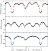 |
Fig. 8. Top: average light curve with the first best-fit photometric solution. Middle: residuals and their best-fit sine wave. Bottom: average light curve after removal of this sine wave, and best-fit photometric solution (solid blue line = supergiant solution, dashed cyan line = giant solution). |
The fitting was restarted on the cleaned light curve, using detailed reflection and performing a large exploration of the parameter space. The parameters of the best-fit photometric solutions are provided in the middle column of Table 2 and shown in the bottom panel of Fig. 8. The errors were calculated assuming the best-fit reduced χ2 corresponds to 1: the range of value for each parameter was then evaluated in all solutions corresponding to reduced χ2 = 1 + 5.89/(N − 5) (1-σ for 5 fitted parameters) or χ2 = 1 + 18.2/(N − 5) (3-σ range), where N = 100, the number of bins in the average light curve. The best-fit periastron argument is in agreement (within the errors) with the spectroscopically derived value and the predicted amplitude of the primary RV curve is 57.1 km s−1, also in excellent agreement with the observed value. The primary radius is however nearly twice too small compared to usual radii of O8.5I supergiants (Martins et al. 2005). It better agrees with a giant classification. The primary bolometric luminosity, derived from its temperature and radius, amounts to log(L/L⊙) = 5.12: it is close to that expected for giant stars, but nearly three times lower than for supergiants (Martins et al. 2005).
Therefore, if we instead consider typical parameters of giant O8.5 stars (temperature of 31.7 kK and mass of 24.84 M⊙, Martins et al. 2005), the mass function from the spectroscopic solution implies secondary masses of 4.5–4.8 M⊙ for inclinations of 90–70° (i.e. q = M2/M1 = 0.18 − 0.19). The fitting was thus restarted considering these values and the best-fit parameters are provided in the last column of Table 2. The predicted amplitude of the primary RV curve now is 57.5 km s−1, and the bolometric luminosities are log(L/L⊙) = 5.07 and 3.71 for the primary and secondary, respectively.
In both cases, if we add the primary luminosity, the companion luminosity (about 4% of the primary luminosity), and the contribution of the third light (about a quarter of the total luminosity, see above), we get a total luminosity of log(L/L⊙)∼5.2. This luminosity still is ∼50% of that derived from the V magnitude, using the bolometric correction of O8.5 giant and supergiant stars and the smallest extinction and distance values.
Finally, we performed a fitting trial fixing the secondary temperature to 15 kK, typical of B5–6V stars with masses similar to that derived for the companion. While the fitting converges towards similar filling factors, inclination, and periastron argument, the deepest eclipse cannot be reproduced hence such a fitting remains unacceptable.
3.3. Constraints from the X-ray analysis
HD 96670 was detected as an X-ray source (XMMSL2 J110714.5–595226) in the XMM slew survey with just four counts, yielding an EPIC-pn count rate of 0.82 ± 0.41 cts s−1 in the 0.2–12. keV energy band (i.e. it is a 2σ detection). It was subsequently re-observed by NuSTAR. Three exposures were taken (ObsID = 30001050002, 4, and 6), with durations between 1 and 2 days, that is, sampling a large part of the orbit. The dates at mid-exposures (HJD = 2 457 086.469, 111.663, and 123.226) correspond to phases of 0.32, 0.09, and 0.28, using our adopted ephemeris (forb = 0.189255 d−1 and T0(conj) = 2 460 064.890). Gomez & Grindlay (2021) reported the fitting of the combined data with a thermal model (kT = 5.2 keV) as well as with a power law (Γ = 2.6), deriving luminosities of ∼2 × 1032 erg s−1 in the 2.–10. keV range. It is not known whether this value corresponds to the observed luminosity or has been corrected for any intervening absorption, but absorption correction is always small for such energies. Considering their distance (2.83 kpc), this corresponds to an (average) flux of ∼2 × 10⁻¹³ erg cm−2 s−1.
Chandra observed HD 96670 in October 2020 (HJD = 2 459 146.154, or ϕ = 0.12). The reddening, E(B − V), of 0.39–0.49 mag corresponds to an absorbing column of 0.24–0.30 × 1022 cm−2 using the formula of Gudennavar et al. (2012). A thermal model (phabsISM × phabs × ∑apec) requires two temperatures, but no additional absorption, to achieve a good fit: NH, ISM = 0.24 × 1022 cm−2, NH = 0 (fixed), kT1 = 0.70 ± 0.17 keV, norm1 = (1.97 ± 0.62)×10−4 cm−5, kT2 = 2.88 ± 0.56 keV, norm2 = (2.95 ± 0.37)×10−4 cm−5, χ2 = 38.51 for 45 degrees of freedom. The observed fluxes are (5.87 ± 0.46) and (2.04 ± 0.26)×10−13 erg cm−2 s−1 in the 0.5–10. keV and 2.–10. keV bands, respectively. For a power law fitting (phabsISM × phabs × pow), we would instead get: NH, ISM = 0.24 × 1022 cm−2, NH = 0 (fixed), Γ = 2.98 ± 0.14, norm = (2.82 ± 0.24)×10−4 cm−5, and χ2 = 61.89 for 49 degrees of freedom. Observed fluxes are (5.43 ± 0.24) and (1.80 ± 0.20)×10−13 erg cm−2 s−1 in 0.5–10. keV and 2.–10. keV, respectively. Those values agree well with the NuSTAR results obtained from the hard band only. It is difficult to distinguish between the thermal and non-thermal scenarios using the available data. Indeed, the iron lines near 6.7 keV (a tell-tale sign of the presence of hot plasma) can only be spotted if there are enough counts at high energies. Unfortunately, this is not the case here.
The thermal fitting provides a better χ2 and its two temperatures appear rather similar to those found for ‘normal’ OB stars, although the hot component here is very strong. In addition, the fluxes corrected for interstellar absorption amount to 8.4 − 8.6 × 10⁻¹³ erg cm−2 s−1 in the 0.5–10. keV band, depending on the chosen model. With the bolometric luminosity of log(L/L⊙) = 5.07 and the smallest distance, this would yield a log(LX/LBOL) of −5.8, about one dex above the usual value of −7 for ‘normal’ massive stars, but much lower than recorded for high-mass X-ray binaries (in outburst). Certainly, the X-rays cannot be due to the sole intrinsic embedded wind-shocks of the primary O star.
The Swift data of HD 96670 were taken at several epochs. It was notably the main target of the exposures taken around the time of the NuSTAR observations. The most secure data correspond to grade = 0, but this additional filtering further reduces the number of counts: there are only 50 counts in the Swift spectrum, making the determination of spectral parameters quite uncertain. A trial was nevertheless attempted. A fitting using a single thermal model yields: NH, ISM = 0.24 × 1022 cm−2 and NH = 0 (both fixed), kT = 0.82 ± 0.13 keV, norm = (1.10 ± 0.18)×10−4 cm−5, χ2 = 5.13 for 3 degrees of freedom, observed fluxes of (1.50 ± 0.27), and (0.12 ± 0.04)×10−13 erg cm−2 s−1 in the 0.5–10. keV and 2.–10. keV bands, respectively. A power law fitting yields: NH, ISM = 0.24 × 1022 cm−2, NH = 0 (fixed), Γ = 2.62 ± 0.38, norm = (1.03 ± 0.17)×10−4 cm−5, χ2 = 6.59 for 3 degrees of freedom, observed fluxes of (2.42 ± 0.90), and (1.07 ± 0.63)×10−13 erg cm−2 s−1 in 0.5–10. keV and 2.–10. keV, respectively. This latter fitting formally is less good than the thermal fitting, but it allows us to catch flux at higher energies (the thermal model fits only the coolest component detected by Chandra, as the sensitivity severely drops at high energies).
While uncertain, it may be noted that those parameters are of the same order of magnitude as those found from Chandra data. As these are broad-band measurements, the count rates should provide more secure information than spectra, at the expense of the spectral resolution. The individual Swift count rates are provided in Table 3 and shown in Fig. 9. Despite uncertainties, HD 96670 seems to display a coherent, phase-locked behaviour, with a larger X-ray flux around ϕ = 0.5 than around ϕ = 0. This conclusion is backed up by the comparison with the XMM slew survey and Chandra results. Indeed, the best-fit power-law fitting of the Chandra spectrum converts7 to an EPIC-pn count rate of ∼0.3 cts s−1 in the 0.2–12. keV band, while the slew catalog provides a value more than twice larger. Considering our ephemeris, the Chandra observations were taken at a phase of 0.12, while the slew exposure is dated from 23 July 2010 (HJD = 2 455 401.392); hence, it has a phase of 0.41. Figure 9 further demonstrates this difference graphically as it displays the equivalent Swift count rates of both the Chandra flux and the XMM slew count rate (using the same Chandra model). All of these results must certainly be confirmed with higher-quality follow-up observations, but it provides a good hint that the X-ray flux of HD 96670 might be variable by a factor of a few over its orbit.
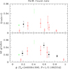 |
Fig. 9. Evolution with orbital phase of the Swift count rates in the 0.5–10. keV band, with the more uncertain values in red (top: for grade = 0 only, bottom: for all grades). Blue tick marks at the bottom indicate the phases of the NuSTAR observations. The green star and the green line indicate the Chandra and XMM slew points, respectively, converted to Swift values. |
Swift count rates in the 0.5–10. keV band.
4. Discussion
It is evident that HD 96670 harbours no black hole, as its light curve displays two eclipses. Instead, the companion is found to be a small, intermediate-mass, and hot object. While its mass may be compatible with a mid B-star, the high temperature and small radius cannot be reconciled with such an object. Such characteristics are much more typical of post-binary interaction systems. For example, the radius and temperature are similar to those observed in known (fully) stripped stars (Wang et al. 2021). We refer, in particular, to the case of ϕ Per, a system containing a Be star and a sdO companion (although the latter object has a smaller mass and a longer period than the secondary of HD 96670 – R2 = 0.9 R⊙, T2 = 53 kK, M2 = 1.2 M⊙, P = 127 d, Mourard et al. 2015).
Figure 10 shows the position of the two components of HD 96670 in the Hertzsprung–Russell diagram (HRD). The position of the primary star in the HRD is compatible with models for slightly evolved 25 M⊙ objects. The primary appears close to the isochrone at 5 Myr, in line with the age of Car OB2 from Garcia (1994). In contrast, the secondary star is located well below the zero age main-sequence hence it is incompatible with single-star evolutionary tracks. However, it appears within the group of known fully stripped stars (see Fig. 10)8. Two different populations form this group in this figure. On the one hand, there are Galactic Be+sdOB systems for which the stripped star is much fainter than its Be companion and has ∼1 M⊙ and Teff = 17 − 53 kK. Their properties were (mostly) constrained through UV spectroscopy, but also via interferometric campaigns and optical spectroscopy (Mourard et al. 2015; Wang et al. 2021; see a summary in Nazé et al. 2022, and references therein). Orbital solutions have been derived for about half of them. On the other hand, there are LMC systems where the stripped star dominates the output flux and has 1–8 M⊙ and Teff = 33 − 90 kK. These stripped stars were detected thanks to a UV photometric excess and their properties were derived from fitting optical spectra with atmosphere models (Götberg et al. 2023). There is no UV spectroscopy or orbital solution available yet for these systems. Considering its mass and temperature, HD 96670 appears to be an intermediate case between these two groups.
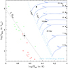 |
Fig. 10. HRD showing the position of the two stars (black dots, Table 2) along with evolutionary tracks of Brott et al. (2011) for the Milky Way and no rotation. Stripped stars properties from Nazé et al. (2022, and references therein) are shown with red triangles and those from Götberg et al. (2023) with green crosses. |
Turning to binary evolutionary models, Götberg et al. (2018) presented a range of stripped star cases. The position of our secondary in the HRD is compatible with those found by these authors, for instance, in the core helium-burning phase of a stripped star with an initial mass of 9 M⊙. This specific model ends up with a stripped star of lower mass, however, Götberg et al. (2018) presented only a limited set of cases (e.g. single mass ratio and single orbital period). A more extensive set can be found in the Binary Population and Spectral Synthesis (BPASS) v2.2.1 database (Eldridge et al. 2017; Stevance et al. 2020). This database was searched for systems with properties similar to ours: solar metallicity (Z = 0.02), period between 3 and 7 d, primary mass between 3 and 7 M⊙, secondary mass between 20 and 30 M⊙, and primary radius between 0.3 and 3 R⊙. We note that the definition of primary and secondary in BPASS is inverted compared to ours since ‘their’ primary corresponds to the initially massive star which has now become the least massive, post-interacting object (i.e. ‘our’ secondary). One BPASS model fulfilled the criteria, namely, a system that started with a 17 + 12 M⊙ pair in a 2.7 d orbit. After 11 Myr, the period becomes 6.9 d. The mass donor now is a stripped star with a temperature of 56–71 kK, a radius of 1.7–2.9 R⊙, and a mass of ∼6 M⊙ while its companion has a temperature of ∼22.4 kK, a radius of ∼8.2 R⊙, and a mass of ∼20.8 M⊙. Of course, this is not a perfect match to the HD 96670 system, but the database remains generic; thus, already finding a relatively close case is a very encouraging start. In this context, we may note that the secondary of HD 96670 also falls amongst the stripped helium stars of the simulations by Yungelson et al. (2024), see in particular their Fig. 4. Although it is beyond the scope of this paper, a more detailed modelling that is specifically tuned to the case of HD 96670 will certainly lead to a better match.
Götberg et al. (2018) calculated typical spectra for stripped stars with a range of temperatures and masses. For 4–5 M⊙ cases, the spectra display a strong and broad emission in He IIλ 4686 Å, small emission components in Balmer lines, and no line at He IIλ 4542 Å. While the secondary of HD 96670 appears cooler than Goetberg’s stars, this may explain why the He IIλ 4542 Å remains uncontaminated, while the profile of He IIλ 4686 Å is complex. Clearly, a denser monitoring of the orbital cycle is needed to understand the behaviour of He IIλ 4686 Å.
While the nature of the system now seems quite clear, a question remains regarding the origin of the X-ray emission. Both massive OB stars and hot subdwarf stars are high-energy sources, but their X-rays are soft and faint, following log(LX/LBOL)∼ − 7 (Nazé et al. 2011; Mereghetti & La Palombara 2016). This is clearly not the case of HD 96670. Regarding stripped stars paired with massive stars, only Be+sdO systems have been examined up to now and no particularly hard or bright X-rays were detected for them9 (Nazé et al. 2022). However, O stars have much stronger winds than the Be stars examined in that paper, while the stripped companion here is more massive. The bright and hard character of the X-rays, coupled to the phase-locked variations hinted by current data, are reminiscent of colliding wind phenomena (for a review, see Rauw 2022). In particular, the X-ray bright part of the colliding winds may be occulted by a large stellar body in high-inclination systems: this could explain the flux decrease seen at ϕ = 0 in HD 96670. Of course, whether and exactly how a colliding wind phenomenon applies to HD 96670 remains to be demonstrated with a sensitive monitoring over the orbital cycle. In addition, a sensitive X-ray exposure would be able to clarify the nature of the high-energy emission; in particular, the presence of a non-thermal component versus a hot thermal component, which would also strongly constrain its origin.
The hypothesis of a wind-wind collision is reinforced by the analysis of the equivalent widths (EW) of the two lines presenting emission components, Hα and He IIλ4686 Å. While the equivalent widths of He I and other He II lines appear rather stable with phase in the FEROS spectra, both contaminated lines show a decrease in their EWs during eclipses (right panel of Fig. 11; the effect appears smaller in Hβ). After an examination of the line profiles (left panels of Figures 1 and 11), it appears that this EW change clearly comes from an increased emission, not from a decreased absorption. This can be understood in the context of colliding winds. Indeed, the shocked plasma is not at the same temperature everywhere in the collision zone, with the highest temperatures (typical of X-ray emitting plasma) usually reached in a small zone near the line-of-centers, while optical lines arise in a very large zone further away from the stars. Such a configuration can explain both a smaller X-ray emission when the large O star hides the small region with the hottest plasma and larger emission components in the optical lines (as the associated emission is diluted by a smaller continuum). These conclusions are encouraging for the colliding wind model, but they remain preliminary, owing to the small number of spectra and the sparse phase coverage.
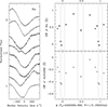 |
Fig. 11. Left: same as Fig. 1 for Hα. Time runs downwards (see Table 1 for exact dates); associated phases are, from top to bottom, 0.97 (2004 data), 0.95, 0.72, 0.92, 0.09, 0.29, 0.49 (2006 data), 0.87 (2009 data). Right: Equivalent widths of Hα (top, black dots) and He IIλ4686 Å (bottom, stars) as a function of phase. These EWs correspond to integration of the profiles in 6545.0–6575.0 Å and 4676.0–4693.5 Å, respectively. The vertical dotted lines correspond to the eclipse limits. |
In conclusion, more studies on HD 96670 are required, but at least the basic parameters of the system have been established. Clearly, additional optical and X-ray monitoring should be performed to improve our understanding of this system and better pinpoint the past and/or current interactions between its components.
Downloaded from the INES database, see http://sdc.cab.inta-csic.es/cgi-ines/IUEdbsMY
The intermediate evolutionary stages such as, e.g., the partially stripped cases reported in Ramachandran et al. (2024, see their Fig. 16) are not shown here.
Except for the subgroup of γ Cas analogs, which do not display phase-locked changes.
Acknowledgments
The authors thank the referee for helpful comments, the Swift helpdesk for their help, and Queen’s music for inspiration (hence the title as hommage). They also acknowledge support from the Fonds National de la Recherche Scientifique (Belgium), the European Space Agency (ESA) and the Belgian Federal Science Policy Office (BELSPO) in the framework of the PRODEX Programme (contracts linked to XMM-Newton and Gaia). This paper includes data collected by the TESS mission, which are publicly available from the Mikulski Archive for Space Telescopes (MAST). Funding for the TESS mission is provided by NASA’s Science Mission directorate. ADS and CDS were used for preparing this document.
References
- Bailer-Jones, C. A. L., Rybizki, J., Fouesneau, M., et al. 2021, AJ, 161, 147 [NASA ADS] [CrossRef] [Google Scholar]
- Bodensteiner, J., Shenar, T., Mahy, L., et al. 2020, A&A, 641, A43 [NASA ADS] [CrossRef] [EDP Sciences] [Google Scholar]
- Bowen, D. V., Jenkins, E. B., Tripp, T. M., et al. 2008, ApJS, 176, 59 [NASA ADS] [CrossRef] [Google Scholar]
- Bowman, D. M., Burssens, S., Simón-Díaz, S., et al. 2020, A&A, 640, A36 [NASA ADS] [CrossRef] [EDP Sciences] [Google Scholar]
- Brott, I., de Mink, S. E., Cantiello, M., et al. 2011, A&A, 530, A115 [NASA ADS] [CrossRef] [EDP Sciences] [Google Scholar]
- Conti, P. S., Leep, E. M., & Lorre, J. J. 1977, ApJ, 214, 759 [Google Scholar]
- El-Badry, K., & Quataert, E. 2020, MNRAS, 493, L22 [NASA ADS] [CrossRef] [Google Scholar]
- El-Badry, K., & Burdge, K. B. 2022a, MNRAS, 511, 24 [NASA ADS] [CrossRef] [Google Scholar]
- El-Badry, K., Burdge, K. B., & Mróz, P. 2022b, MNRAS, 511, 3089 [NASA ADS] [CrossRef] [Google Scholar]
- Eldridge, J. J., Stanway, E. R., Xiao, L., et al. 2017, PASA, 34, e058 [Google Scholar]
- Fortin, F., García, F., Simaz Bunzel, A., et al. 2023, A&A, 671, A149 [NASA ADS] [CrossRef] [EDP Sciences] [Google Scholar]
- Garcia, B. 1993, ApJS, 87, 197 [NASA ADS] [CrossRef] [Google Scholar]
- Garcia, B. 1994, ApJ, 436, 705 [NASA ADS] [CrossRef] [Google Scholar]
- Gies, D. R., & Wang, L. 2020, ApJ, 898, L44 [NASA ADS] [CrossRef] [Google Scholar]
- Gomez, S., & Grindlay, J. E. 2021, ApJ, 913, 48 [NASA ADS] [CrossRef] [Google Scholar]
- González, J. F., & Levato, H. 2006, A&A, 448, 283 [NASA ADS] [CrossRef] [EDP Sciences] [Google Scholar]
- Gosset, E., Royer, P., Rauw, G., et al. 2001, MNRAS, 327, 435 [NASA ADS] [CrossRef] [Google Scholar]
- Götberg, Y., de Mink, S. E., Groh, J. H., et al. 2018, A&A, 615, A78 [NASA ADS] [CrossRef] [EDP Sciences] [Google Scholar]
- Götberg, Y., Drout, M. R., Ji, A. P., et al. 2023, ApJ, 959, 125 [CrossRef] [Google Scholar]
- Gudennavar, S. B., Bubbly, S. G., Preethi, K., et al. 2012, ApJS, 199, 8 [NASA ADS] [CrossRef] [Google Scholar]
- Harmanec, P., Holmgren, D. E., Wolf, M., et al. 2014, A&A, 563, A120 [NASA ADS] [CrossRef] [EDP Sciences] [Google Scholar]
- Heck, A., Manfroid, J., & Mersch, G. 1985, A&AS, 59, 63 [NASA ADS] [Google Scholar]
- Jones, C. E., Labadie-Bartz, J., Cotton, D. V., et al. 2022, Ap&SS, 367, 124 [NASA ADS] [CrossRef] [Google Scholar]
- Kołaczek-Szymański, P. A., Pigulski, A., Michalska, G., et al. 2021, A&A, 647, A12 [NASA ADS] [CrossRef] [EDP Sciences] [Google Scholar]
- Lamberts, A., Garrison-Kimmel, S., Hopkins, P. F., et al. 2018, MNRAS, 480, 2704 [NASA ADS] [CrossRef] [Google Scholar]
- Lanz, T., & Hubeny, I. 2003, ApJS, 146, 417 [NASA ADS] [CrossRef] [Google Scholar]
- Mahy, L., Sana, H., Shenar, T., et al. 2022, A&A, 664, A159 [NASA ADS] [CrossRef] [EDP Sciences] [Google Scholar]
- Martins, F., & Plez, B. 2006, A&A, 457, 637 [NASA ADS] [CrossRef] [EDP Sciences] [Google Scholar]
- Martins, F., Schaerer, D., & Hillier, D. J. 2005, A&A, 436, 1049 [NASA ADS] [CrossRef] [EDP Sciences] [Google Scholar]
- Mereghetti, S., & La Palombara, N. 2016, Advances in Space Research, 58, 809 [Google Scholar]
- Miller-Jones, J. C. A., Bahramian, A., Orosz, J. A., et al. 2021, Science, 371, 1046 [Google Scholar]
- Mourard, D., Monnier, J. D., Meilland, A., et al. 2015, A&A, 577, A51 [NASA ADS] [CrossRef] [EDP Sciences] [Google Scholar]
- Nazé, Y., Broos, P. S., Oskinova, L., et al. 2011, ApJS, 194, 7 [CrossRef] [Google Scholar]
- Nazé, Y., Rauw, G., & Gosset, E. 2021, MNRAS, 502, 5038 [CrossRef] [Google Scholar]
- Nazé, Y., Rauw, G., Smith, M. A., et al. 2022, MNRAS, 516, 3366 [CrossRef] [Google Scholar]
- Nazé, Y., Britavskiy, N., Rauw, G., et al. 2023, MNRAS, 525, 1641 [CrossRef] [Google Scholar]
- Olejak, A., Belczynski, K., Bulik, T., et al. 2020, A&A, 638, A94 [NASA ADS] [CrossRef] [EDP Sciences] [Google Scholar]
- Ramachandran, V., Sander, A. A. C., Pauli, D., et al. 2024, A&A, 692, A90 [NASA ADS] [CrossRef] [EDP Sciences] [Google Scholar]
- Rauw, G. 2022, Handbook of X-ray and Gamma-ray Astrophysics, 108 [Google Scholar]
- Rauw, G., & Nazé, Y. 2016, A&A, 594, A82 [NASA ADS] [CrossRef] [EDP Sciences] [Google Scholar]
- Rauw, G., & Nazé, Y. 2021, MNRAS, 500, 2096 [Google Scholar]
- Ricker, G. R., Winn, J. N., Vanderspek, R., et al. 2015, Journal of Astronomical Telescopes Instruments, and Systems, 1, 014003 [Google Scholar]
- Rivinius, T., Klement, R., Chojnowski, S. D., et al. 2024, IAU Symposium, 361, 332 [Google Scholar]
- Rosu, S., Rauw, G., Nazé, Y., et al. 2022, A&A, 664, A98 [NASA ADS] [CrossRef] [EDP Sciences] [Google Scholar]
- Sana, H., Le Bouquin, J.-B., Lacour, S., et al. 2014, ApJS, 215, 15 [Google Scholar]
- Savage, B. D., Meade, M. R., & Sembach, K. R. 2001, ApJS, 136, 631 [NASA ADS] [CrossRef] [Google Scholar]
- Saxton, R. D., Read, A. M., Esquej, P., et al. 2008, A&A, 480, 611 [NASA ADS] [CrossRef] [EDP Sciences] [Google Scholar]
- Simón-Díaz, S., & Herrero, A. 2007, A&A, 468, 1063 [NASA ADS] [CrossRef] [EDP Sciences] [Google Scholar]
- Sota, A., Maíz Apellániz, J., Walborn, N. R., et al. 2011, ApJS, 193, 24 [Google Scholar]
- Sota, A., Maíz Apellániz, J., Morrell, N. I., et al. 2014, ApJS, 211, 10 [Google Scholar]
- Stevance, H., Eldridge, J., & Stanway, E. 2020, The Journal of Open Source Software, 5, 1987 [Google Scholar]
- Stickland, D. J., & Lloyd, C. 2001, The Observatory, 121, 1 [NASA ADS] [Google Scholar]
- Thackeray, A. D., Tritton, S. B., & Walker, E. N. 1973, MmRAS, 77, 199 [NASA ADS] [Google Scholar]
- Wang, L., Gies, D. R., Peters, G. J., et al. 2021, AJ, 161, 248 [Google Scholar]
- Wichmann, R. 2011, Astrophysics Source Code Library [record ascl:1106.016] [Google Scholar]
- Yungelson, L., Kuranov, A., Postnov, K., et al. 2024, A&A, 683, A37 [NASA ADS] [CrossRef] [EDP Sciences] [Google Scholar]
All Tables
All Figures
|
Fig. 1. Left and middle panels: various lines recorded in the eight FEROS spectra, with arbitrary vertical shifts to make differences clearer (oldest spectrum on top, earliest at bottom). Right: lines corrected for the average He II velocity (Table 1): He II and C IV display no profile change, while H and He I do. |
| In the text | |
|
Fig. 2. RVs measured on FEROS data from different sets of lines. |
| In the text | |
|
Fig. 3. Left: RVs of HD 96670 used by Stickland & Lloyd (2001: black dots), averages of the RVs derived by Gomez & Grindlay (2021: blue triangles), and RVs measured on FEROS data (red stars). The Stickland & Lloyd solution is also shown – beware that the period used by these authors was different. The bottom panel displays the average TESS LC, phased with the same ephemeris. Right: shifted RVs along with the solutions of Stickland & Lloyd (black line, with γ set to zero) and ours (dotted green line). Here, ϕ = 0 corresponds to conjunction with the O star in front and only the FEROS points from 2006 (marked with an asterisk in Table 1) are shown. |
| In the text | |
|
Fig. 4. Difference between RVs of HD 96670 and the solution of Stickland & Lloyd (2001). |
| In the text | |
|
Fig. 5. Results of the disentangling applied to the six FEROS spectra from 2006, keeping the RVs fixed and assuming q = 0.18. The reconstructed spectra of the primary (blue) and secondary (red) are normalized against the combined continuum of the system. For clarity, the normalized secondary spectrum is shifted vertically by 0.2. |
| In the text | |
|
Fig. 6. TESS light curves of HD 96670, and their associated periodograms. Dotted red lines in the right panels indicate the orbital frequency and its harmonics. |
| In the text | |
|
Fig. 7. Binned light curves for the three TESS observing campaigns (left) and for the Gomez & Grindlay photometry (middle, a zero point of 7.62 was subtracted) using forb = 0.189250 d−1. Error bars correspond to a 1σ dispersion in each bin. Right: Same as left panel but using forb = 0.189255 d−1 (the spectroscopic one). |
| In the text | |
|
Fig. 8. Top: average light curve with the first best-fit photometric solution. Middle: residuals and their best-fit sine wave. Bottom: average light curve after removal of this sine wave, and best-fit photometric solution (solid blue line = supergiant solution, dashed cyan line = giant solution). |
| In the text | |
|
Fig. 9. Evolution with orbital phase of the Swift count rates in the 0.5–10. keV band, with the more uncertain values in red (top: for grade = 0 only, bottom: for all grades). Blue tick marks at the bottom indicate the phases of the NuSTAR observations. The green star and the green line indicate the Chandra and XMM slew points, respectively, converted to Swift values. |
| In the text | |
|
Fig. 10. HRD showing the position of the two stars (black dots, Table 2) along with evolutionary tracks of Brott et al. (2011) for the Milky Way and no rotation. Stripped stars properties from Nazé et al. (2022, and references therein) are shown with red triangles and those from Götberg et al. (2023) with green crosses. |
| In the text | |
|
Fig. 11. Left: same as Fig. 1 for Hα. Time runs downwards (see Table 1 for exact dates); associated phases are, from top to bottom, 0.97 (2004 data), 0.95, 0.72, 0.92, 0.09, 0.29, 0.49 (2006 data), 0.87 (2009 data). Right: Equivalent widths of Hα (top, black dots) and He IIλ4686 Å (bottom, stars) as a function of phase. These EWs correspond to integration of the profiles in 6545.0–6575.0 Å and 4676.0–4693.5 Å, respectively. The vertical dotted lines correspond to the eclipse limits. |
| In the text | |
Current usage metrics show cumulative count of Article Views (full-text article views including HTML views, PDF and ePub downloads, according to the available data) and Abstracts Views on Vision4Press platform.
Data correspond to usage on the plateform after 2015. The current usage metrics is available 48-96 hours after online publication and is updated daily on week days.
Initial download of the metrics may take a while.