| Issue |
A&A
Volume 696, April 2025
|
|
|---|---|---|
| Article Number | A9 | |
| Number of page(s) | 11 | |
| Section | Astrophysical processes | |
| DOI | https://doi.org/10.1051/0004-6361/202453158 | |
| Published online | 28 March 2025 | |
Probing the interstellar medium toward GRB 221009A through X-ray dust scattering
1
Scuola Universitaria Superiore IUSS Pavia, Piazza della Vittoria 15, 27100 Pavia, Italy
2
Department of Physics, University of Trento, Via Sommarive 14, 38123 Povo, (TN), Italy
3
INAF – Istituto di Astrofisica Spaziale e Fisica Cosmica di Milano, Via A. Corti 12, 20133 Milano, Italy
4
Ruder Bošković Institute, Bijenič ka cesta 54, 10000 Zagreb, Croatia
5
University of Zagreb Faculty of Electrical Engineering and Computing, Unska ul. 3, 10000 Zagreb, Croatia
6
INAF – Osservatorio Astrofisico di Arcetri, Largo E. Fermi 5, 50125 Firenze, Italy
7
Laboratoire de Physique de l’Ecole Normale Supérieure, ENS, Université PSL, CNRS, Sorbonne Université, Université de Paris, F-75005 Paris, France
8
INAF – Osservatorio Astronomico di Brera, Via Bianchi 46, 23807 Merate, (LC), Italy
9
Center for Astrophysics | Harvard & Smithsonian, 60 Garden Street, Cambridge, MA 02138, USA
⋆ Corresponding author; This email address is being protected from spambots. You need JavaScript enabled to view it.
Received:
25
November
2024
Accepted:
28
February
2025
Abstract
The observation of 21 X-ray dust-scattering rings around the extraordinarily bright gamma-ray burst (GRB) 221009A provides a unique opportunity to study the interstellar medium (ISM) through which the X-ray radiation traveled in our Galaxy and, by extension, in the host galaxy as well. In particular, since the ring intensity and radius at a given time depend on the amount of dust and on its distance, respectively, XMM-Newton and Swift images allowed us to map the ISM around the direction of the GRB with better resolution than in the existing optical- and infrared-based 3D dust maps, both in the plane of the sky (a few arcminutes) and along the line of sight (from ≃1 pc for dust clouds within 1 kpc to ≃100 pc for structures at distances larger than 10 kpc). As a consequence, we could revise prior estimates of the GRB soft X-ray fluence, obtaining a ∼35% lower value, which, however, still indicates a substantial excess with respect to the extrapolation of the spectral models constrained by hard X-ray observations. Additionally, we detect significant spectral variability in two azimuthal sectors of the X-ray rings, which can be fully attributed to different Galactic absorption in these two directions. The comparison of the total hydrogen column density inferred from spectral fitting, with the Galactic contribution derived from the intensity of the X-ray rings, in the same sectors allowed us to more robustly constrain the absorption in the host galaxy to NH, z = 0.151 = (3.7 ± 0.3)×1021 cm−2. This result is relevant not only for characterizing the ISM of the host galaxy and understanding how the GRB radiation might have affected it, but also for modeling the broadband spectrum of the GRB afterglow and constraining the properties of a possible underlying supernova.
Key words: dust / extinction / X-rays: ISM / gamma-ray burst: individual: GRB 221009A
© The Authors 2025
 Open Access article, published by EDP Sciences, under the terms of the Creative Commons Attribution License (https://creativecommons.org/licenses/by/4.0), which permits unrestricted use, distribution, and reproduction in any medium, provided the original work is properly cited.
This article is published in open access under the Subscribe to Open model. This email address is being protected from spambots. You need JavaScript enabled to view it. to support open access publication.
1. Introduction
Gamma-ray burst (GRB) 221009A is the brightest GRB ever recorded (Burns et al. 2023). It occurred in a direction close to the Galactic plane (b = 4° .32, l = 52° .96), resulting in the formation of 21 X-ray rings due to scattering by interstellar dust in our Galaxy (Tiengo et al. 2023, hereafter T23; Vasilopoulos et al. 2023; Williams et al. 2023; Zhao & Shen 2024).
In the Milky Way, dust comprises only about 1% of the total mass of the interstellar medium (ISM) (Bohlin et al. 1978); the majority of the ISM mass is gas, found in both atomic and molecular forms. Despite its small mass fraction, dust has a significant impact on astrophysical processes in all galaxies. Dust grains contribute to cooling effects that influence star and planet formation (see, e.g., Schneider et al. 2002; Johansen & Lambrechts 2017) and provide surfaces for chemical reactions, facilitating the formation of complex molecules. Dust also has a strong impact on many astronomical observations. First, it causes the extinction of radiation, mainly in the optical and UV wavebands, which, for extragalactic objects, requires a correction that accounts for dust both in our Galaxy and in the host galaxy. Second, the thermal emission of interstellar dust contaminates astronomical observations at long wavelengths, significantly affecting, in particular, the study of the cosmic microwave background.
In X-ray astronomy, dust impacts observations by absorbing and scattering X-ray photons. Although X-ray absorption is dominated by the contribution of gas metals in the ISM, high-resolution spectroscopy makes it possible to isolate the contribution of some dust constituents or to infer their presence from the abundances of specific elements, such as iron or oxygen (see, e.g., Psaradaki et al. 2023). When only low-resolution X-ray spectra are available, the quantity of dust along the line of sight can be estimated by modeling the photoelectric X-ray absorption and making assumptions on the dust-to-gas ratio.
Dust scattering of X-rays from bright point sources is a well-known and thoroughly studied phenomenon. For steady sources, this scattering produces a diffuse halo around the source at soft X-ray energies (Predehl & Schmitt 1995; Smith 2008). However, if the source undergoes a distinct flare followed by a period of quiescence, the scattering instead appears as discrete rings (Vaughan et al. 2004; Tiengo et al. 2010; Heinz et al. 2016; Pintore et al. 2017) that expand over time. The angular size of the formed expanding ring, θ, is given by the relation
 (1)
(1)
where c is the speed of light, Δt is the time delay between the direct and scattered X-rays, Ds is the distance to the X-ray source, and Dd is the distance to the dust cloud (Miralda-Escudé 1999). In the case of GRBs scattered by Galactic dust, the distance to the X-ray source, Ds, is much greater than the distance to the dust layer, Dd. Under these circumstances, Dd/Ds becomes very small, and the expression for the angle θ simplifies to
![Mathematical equation: $$ \begin{aligned} \theta [\mathrm{arcmin}]= 4.455\sqrt{\frac{\Delta t[\mathrm{days}]}{D_{\rm s}[\mathrm{kpc}]}}. \end{aligned} $$](/articles/aa/full_html/2025/04/aa53158-24/aa53158-24-eq2.gif) (2)
(2)
The flux of the ring, as a function of energy (E), due to the single scattering of GRB photons in a thin dust cloud within our Galaxy, and observed to expand from θ1 to θ2, can be described as
 (3)
(3)
where F(E) is the GRB specific fluence, Texp is the observation duration, ΔNH is the equivalent hydrogen column density of dust in the cloud averaged over the entire ring, and σθ1, 2(E) is the scattering cross section integrated between θ1 and θ2. Therefore, observing X-ray rings allows us to study both the properties of the source and the intervening dust. T23 derived the fluence and spectrum of the soft X-ray emission of GRB 221009A from observations of its dust-scattering rings performed a few days after the GRB with the European Photon Imaging Camera (EPIC; Strüder et al. 2001; Turner et al. 2001) on board the X-ray Multi Mirror (XMM) Newton satellite. Here we used the same dataset, supplemented with observations by the X-Ray Telescope (XRT; Burrows et al. 2005) on board the Neil Gehrels Swift Observatory (Gehrels et al. 2004), to study the distribution of interstellar dust responsible for scattering, both along the line of sight and in the plane of the sky. GRB 221009A presents a unique opportunity to investigate the Galactic ISM through X-ray scattering and absorption thanks to the combination of its exceptional fluence and its ideal position in Galactic coordinates. A GRB with this luminosity occurring at such a close distance is estimated to be a once-in-10 000-year event (Burns et al. 2023), and its line of sight intercepts all the Milky Way spiral arms up to a distance of nearly 20 kpc from us (Vasilopoulos et al. 2023; Williams et al. 2023; T23). The paper is organized as follows: Section 2 details the reduction of the observations, Sect. 3 outlines the analysis, Sect. 4 discusses the results, and Sect. 5 presents our conclusions.
2. Observations and data reduction
In this study we examined Swift/XRT and XMM-Newton observations of GRB 221009A, performed between October 10 and October 14. The associated observation IDs are presented in Table 1. In later time observations, only the rings produced by the most distant clouds were fully covered (see Eq. (2)), while here we mostly focus on clouds within 800 pc, which can also be identified through optical extinction. On the other side, Swift exposures taken within 1 day from the GRB discovery were not considered because the windowed-timing mode was used and no 2D images were produced.
2.1. XMM-Newton
XMM-Newton observed GRB 221009A for 50 ks on October 11, 2022 (Obs1) and for 62 ks on October 14, 2022 (Obs2). For minimizing pileup in Obs1 the EPIC pn (Strüder et al. 2001) and the two EPIC metal oxide semiconductors (MOSs; Turner et al. 2001) cameras were operated in timing mode, with the thick optical-blocking filter. In timing mode, only the peripheral CCDs of the MOS cameras offer full imaging capabilities from ∼5′ to ∼15′, from the target position. In Obs2 all the EPIC cameras were in full-frame mode and the thin optical filter was used. The second part of this observation was affected by strong and variable particle background. Therefore, we limited the analysis to the longest uninterrupted time interval with quiescent background, resulting in a net exposure time of 33.5 ks for the MOS2 and 29.7 ks for the pn. We do not report the analysis of the MOS1 data for either observation due to the permanent damage sustained by two external CCDs during the early stages of the mission.
XMM-Newton observed the GRB three additional times on October 30, November 1, and November 11, 2022 (Observation IDs: 0913991701, 0913991801, and 0913991901). In these observations, only the rings produced by the most distant clouds (Dd > 3 kpc) are visible, and therefore we used them only for subtracting the background in the analysis reported in Appendix A.
To subtract the contribution from the X-ray background as well as from the GRB afterglow and its possible dust-scattering halo in Obs2, without any contamination from X-ray rings, we searched for archival observations of extragalactic point sources with similar flux and spectrum, and behind a significant amount of Galactic dust. As our best choice, we selected an observation of the bright high-redshift quasar RBS 315 (Observation ID: 0690900201) performed in January 2013, at a similar phase of the Solar Cycle, in order to have a similar contamination from the unfocused particle background (Gastaldello et al. 2022). This quasar is located in a relatively dusty region (Av = 0.7; Schlafly & Finkbeiner 2011) and was observed by XMM-Newton in full-frame mode with the thin filter, as in Obs2 (see Appendix B for further details).
The data were processed using Science Analysis Software (SAS) 20.0.0 (Gabriel et al. 2004) and the latest calibration files. The EPIC events were cleaned with standard filtering expressions1. To maximize the signal-to-noise ratio of the rings, the analysis was confined to the 0.7–4 keV energy band, as in T23. Point-like sources were removed by excluding circular regions after running the SAS source detection task emldetect. For the spectral analysis response matrices were generated using the SAS tasks rmfgen and arfgen.
2.2. Swift-XRT
We analyzed Swift observations of GRB 221009A made with XRT from October 10 to October 13, all taken in photon-counting mode. The corresponding observation IDs are listed in Table 1. Additionally, we used late-time observations of the GRB performed in March and April 2023 (observation IDs from 01126853076 to 01126853084) to create a single sky background event file. We also employed observations from October 25–29, 2022 (Observation IDs 01126853023 to 01126853027), where the GRB afterglow was still present but the rings were sufficiently large and faint, to isolate the afterglow contribution (see Appendix B for details). The data were processed with standard procedures using the FTOOLS task xrtpipeline. Point-like sources were removed by excluding circular regions after source detection (we chose to exclude point-like sources with a signal-to-noise ratio > 3). For the spectral analysis the redistribution matrix file (RMF) was obtained from the calibration database released on 01-01-2013 and the ancillary response files (ARFs) were created using the task xrtmkarf (imposing psfcorr=no).
Log of the Swift/XRT and XMM-Newton observations of GRB 221009A.
3. Data analysis and results
Since Swift/XRT began observing GRB 221009A in photon-counting mode one day after the burst, it could observe rings formed by dust clouds at heliocentric distances smaller than 300 pc, which were already outside the EPIC field of view (FOV) during the XMM-Newton observations (see Eq. (2)). Unfortunately, due to the telescope’s off-axis pointing, we were not able to observe these rings across the entire Swift/XRT FOV, only within a 105° wide sector (290° −395°, measured counterclockwise from west), which extended up to 14′ from the GRB. This sector, which we call Sector 1 (see Fig. 1), represents therefore the only region in which we can map the dust distribution throughout the whole Galaxy (from ∼0.1 to ∼20 kpc). As noted in T23, there are significant variations in the azimuthal distribution of the surface brightness of the brightest X-ray rings, which can be explained by the nonuniform distribution of dust in the intervening clouds. To exploit this azimuthal variation, we selected another sector with the same size as Sector 1 (Sector 2; see Fig. 1). The selection of this sector was driven by the analysis of X-ray absorption in Obs2 (see Appendix A), which showed that Sector 2 (75° −180°) is the only region with a significant NH excess. This result is confirmed also by the total NH map of the GRB 221009A region estimated from Planck submillimeter data of thermal dust emission (see Fig. 4 in T23).
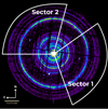 |
Fig. 1. Combined XMM-Newton X-ray observations of GRB 221009A, with the two sectors used for our analysis highlighted. |
3.1. Galactic dust distribution
In Sectors 1 and 2, we analyzed the expanding dust-scattering rings using the pseudo-distance distribution (Tiengo & Mereghetti 2006), which we briefly summarize in the following. For each detected event, we computed the time delay of the photons respect to the GRB time (ti) and the angle between the scattered photon and the source direction (θi):
 (4)
(4)
 (5)
(5)
where xi, yi, and Ti are the detector coordinates and the time of arrival of the i-th event, and T0, XGRB, and YGRB are the GRB time (59861.55568 MJD) and detector coordinates, respectively. Using these new coordinates, we computed the pseudo-distance defined as
![Mathematical equation: $$ \begin{aligned} D_{{i}} = 2ct_{{i}} / \theta _{{i}}^2 = 827\,t_{{i}}\, [s] \,\theta _{{i}}^{-2}\,[\mathrm{arcsec}]\, \mathrm{\,pc} .\end{aligned} $$](/articles/aa/full_html/2025/04/aa53158-24/aa53158-24-eq6.gif) (6)
(6)
For events that are not related to dust-scattered photons, this quantity does not represent a true physical distance. However, for photons from a ring that expands according to Eq. (2), the pseudo-distance, Di, corresponds to the distance of the dust grains that scattered them. Consequently, all the X-rays scattered by a given dust cloud are detected at times and positions corresponding to approximately the same values of Di, resulting in a peak in the pseudo-distance distribution at the cloud’s distance.
After constructing the histogram of the pseudo-distances for each sector (already presented in T23 for the whole FOV) and subtracting the background (see Appendix B), we transformed this count distribution C(D) into the equivalent hydrogen column density of the dust ΔNH(D). This parameter can be obtained from our spectral model because the dust model is normalized to the number of hydrogen atoms (Zubko et al. 2004). For this transformation we used a conversion factor f(θ, t) that must be computed separately for every angular distance from the GRB position (θ) and for each observation, accounting for the time elapsed since the GRB (t), the exposure duration and the detector efficiency. The procedure we used to compute such conversion factors is described in Appendix C.
Applying these conversion factors, we obtained the differential hydrogen column density distribution shown in Fig. 2 for the two sectors in the two MOS2 datasets and only for Sector 1 in the combined XRT observations (see Table 1), which allow us to sample nearby dust. The NH distributions obtained across the entire FOV for both MOS and pn cameras were compared and found to be consistent. However, in this work, we report the ΔNH maps only for the MOS2 camera, as it provides better coverage of Sector 1. Figure 2 demonstrates that the various datasets within the same sector are compatible with each other.
Due to the short duration of the GRB prompt emission, the brightness of the X-ray rings in different observations does not depend on the time variability of the source, but only on the spatial distribution of dust and on the angular dependence of the scattering cross section, according to the selected dust model. To evaluate the azimuthal uniformity of the dust clouds at different angular distances (θ), we generated the diagrams in Fig. 3, which display the integrated NH for the four main peaks in Fig. 2 observed by both the Swift and XMM-Newton satellites. In these charts, data for Sector 1 are represented as positive values of θ, while the data for the other sector are shown as negative values. To reduce uncertainties, Swift observations from multiple orbits were merged. From these figures, it is evident that the clouds at 406 pc, 550 pc, and the cloud complex at 700 pc contain more dust in Sector 2 than in Sector 1. On the contrary, for the cloud at 475 pc, we do not detect any significant variability. The inset of the last panel in Fig. 3 illustrates the contributions of the two clouds within the cloud complex at ∼700 pc in Sector 1: the cloud at 729 pc dominates up to 10′, but at larger angular distances, covered by the second XMM-Newton observation, the corresponding X-ray rings fade away and the contribution from the cloud at 695 pc becomes predominant.
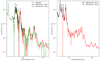 |
Fig. 2. Left: differential hydrogen column density in Sector 1. The Swift-XRT data are in green, the data obtained with the first XMM-Newton observation in black, and the data obtained with the second XMM-Newton observation in red. Right: Differential hydrogen column density in Sector 2. The data obtained with the first XMM-Newton observation are in black, and the data obtained with the second XMM-Newton observation in red. The blue arrows highlight the four main peaks observed by both XMM-Newton and Swift. |
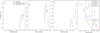 |
Fig. 3. Hydrogen column density obtained by integrating the pseudo-distance distribution at the four main peaks in Fig. 2 (highlighted with blue arrows), centered at 406.3 pc (leftmost panel), 475.2 pc (center-left panel), 553.6 pc (center-right panel), and ∼700 pc (rightmost panel). The inset of the last panel shows the two clouds around 700 pc as separate values: the circles refer to the peak at 695.4 pc (Swift-XRT in blue, XMM-Newton in brown for Obs1, and pink for Obs2), and the squares to the peak centered at 728.6 pc (Swift-XRT in green, XMM-Newton in black for Obs1, and red for Obs2). In all the other panels the values from Swift-XRT observations are shown in green, and from XMM-Newton observations in black (Obs1) and red (Obs2). |
3.2. Absorption in the host galaxy
In addition to the variation in ring intensity across the two different sectors (discussed in Sect. 3.1), we also detect spectral differences, which, as already shown in Appendix A, can be explained by a different amount of Galactic absorption. The combined analysis of the spatially resolved intensity and absorption of the dust-scattered X-ray emission of GRB 221009A enables us to distinguish between Galactic absorption and the contribution from the host galaxy. Specifically, the intensity of the X-ray rings enables the quantification of dust along the line of sight within our Galaxy, while the X-ray absorption in the ring spectra is produced by the combined effect of the ISM both in our Galaxy and in the host galaxy. By assuming a dust-to-gas ratio and subtracting these values, we can determine the amount of dust (and gas) present in the host galaxy.
To calculate the total X-ray absorption for each sector, we selected the annular regions with the largest signal-to-noise ratio. We extracted the ring spectra from the first XMM-Newton observation within the angular ranges from 8′ to 9′ (covering the two rings produced by dust at distances of 695 and 728 pc) and from 9′ to 12′ (including three rings formed by dust at 406, 439, and 475 pc). For the second XMM-Newton observation, we extracted the spectra in the angular range from 11′ to 12′ (containing the two rings generated by dust at 695 and 728 pc), utilizing data from both the MOS2 and pn cameras. For each spectrum, the background was extracted from the same detector region in the RBS 315 observation. We fit simultaneously the spectra of each ring with the XSPEC model CONSTANT × TBABS × RINGSCAT × PEGPWRLW, where, at odds with the model described in Appendix A, TBABS includes the cumulative absorption from the ISM in our Galaxy and in the host galaxy. The angles in the RINGSCAT spectral component were fixed to the limits of each ring and all the other spectral parameters, except for NH in TBABS and the value of the CONSTANT2, were linked to the same values for the spectra of the two sectors. With this model, we obtained a good fit: χ2/d.o.f. = 140.4/150, corresponding to a null-hypothesis probability (nhp) of 96.5% (for a more detailed description of the model and an example of the best-fit spectrum refer to T23). The best-fit photon index of the power-law component (Γ = 1.38 ± 0.05) is perfectly consistent with the one derived, making similar assumptions, in T23 for the full rings and, as anticipated by the preparatory work in Appendix A, the absorption in the two sectors is significantly different: NH, abs 1 = (9.6 ± 0.2)×1021 cm−2 and NH, abs 2 = (12.0 ± 0.2)×1021 cm−2 for sector 1 and 2, respectively. This confirms that the spectral differences between the two sectors can be fully attributed to Galactic X-ray absorption, and we do not find any evidence of a different scattering cross section in the two sectors. Significant spectral differences would be expected in the case of strong spatial variability of the dust population (see, e.g., the spectral parameters obtained in T23 for different dust models) or for nonspherical grains (Draine & Allaf-Akbari 2006).
For both sectors, we produced the cumulative NH in our Galaxy from ring emission (left panel of Fig. 4) by integrating the corresponding pseudo-distance distributions, starting from the largest distances. To complete the cumulative distribution for Sector 2, we assumed the same dust concentration as in Sector 1 for distances smaller than 300 pc. We utilized Swift data up to 300 pc, Obs1 data up to 900 pc, and, beyond 900 pc, we used data derived from Obs2. The total integrated values for sector 1 and 2 are NH, sca 1 = (4.34 ± 0.04)×1021 cm−2 and NH, sca 2 = (5.54 ± 0.04) × 1021cm−2, respectively.
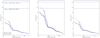 |
Fig. 4. Cumulative hydrogen column density in our Galaxy for Sector 1 (solid black lines) and Sector 2 (solid blue lines) derived from ring emission under different assumptions: GRB fluence from T23 (left panel); 1.9 times lower fluence than in T23 (middle panel); GRB fluence from T23 and 2.6 times more dust in Sector 2 than in Sector 1 within 300 pc (right panel). In the first two panels, the same dust concentration is assumed for both sectors at distances < 300 pc. The dashed lines (black for Sector 1, blue for Sector 2) indicate the total hydrogen column density, including contributions from both our Galaxy and the host galaxy, measured from the absorption inferred from X-ray spectral fitting. |
Although the difference between the final value of the cumulative dust distribution (ΔNH, sca = NH, sca 2 − NH, sca 1) and the total X-ray absorption (ΔNH, abs = NH, abs 2 − NH, abs 1) in the two sectors should be consistent, since it does not depend on the absorption in the host galaxy, we found significantly different values: ΔNH, sca = (1.20 ± 0.06)×1021 cm−2 and ΔNH, abs = (2.4 ± 0.3)×1021 cm−2.
This discrepancy is likely due to some of the assumptions made during the computation of the cumulative dust map (NH, sca). For instance, as described in Appendix C, we adopted a GRB fluence based on the values reported in T23. However, this measurement is affected by the systematic uncertainties discussed in Sect. 4.4. Since NH, sca is inversely proportional to the GRB fluence (see Eq. (3)), to reconcile the observed values, we could assume a 1.9 times lower GRB fluence. This adjustment results in the cumulative distributions shown in the central panel of Fig. 4 and an absorption in the host galaxy of NH, z = 0.151(1.8 ± 0.3)×1021 cm−2. The second assumption involves the extrapolation to small distances for the cumulative distribution of Sector 2, which is assumed to be the same as that of Sector 1. By instead assuming an excess of dust by a factor of 2.6 in the dust clouds at distances smaller than 300 pc in Sector 2, we obtain the cumulative dust distributions shown in the right panel of Fig. 4, and the resulting absorption in the host galaxy is NH, z = 0.151 = (7.0 ± 0.3) × 1021 cm−2. A more robust estimate of NH, z = 0.151 can be derived from the detailed comparison of our dust distance distributions with 3D optical extinction maps, which will be discussed in the next section.
4. Discussion
We can compare the dust map derived from X-ray scattering with other maps generated in the direction of GRB 221009A using data at various wavelengths. Here we focus on the 3D extinction maps from Lallement et al. (2022), Edenhofer et al. (2024), and Green et al. (2019).
4.1. Comparison with the Lallement map
The extinction map constructed by Lallement et al. (2022) integrates Gaia Early Data Release 3 (EDR3) and 2MASS photometric data with Gaia EDR3 parallaxes. This map has a distance resolution of 25 pc and an angular resolution greater than 1° in the plane of the sky3.
This angular resolution is not sufficient to separately probe the directions of the two sectors sampled by the X-ray data. However, most extinction increases in the Lallement et al. (2022) map extracted in the direction of GRB 221009A occur at the same distances as the peaks of the pseudo-distance distributions of the two sectors (left panel of Fig. 5). This confirms the results reported by Šiljeg et al. (2023) for the dust distribution averaged over the full FOV.
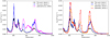 |
Fig. 5. Differential hydrogen column density derived from X-ray dust scattering for Sector 1 (black) and Sector 2 (blue), compared to 3D optical extinction maps. Left: Values derived by Lallement et al. (2022), displayed in pink. Right: Differential hydrogen column density from Edenhofer et al. (2024) for Sector 1 (in orange) and Sector 2 (in red). A conversion factor of 1.9 × 1021 cm−2 mag−1 between NH and Av was used. |
Thanks to the conversion factors described in Appendix A and adopting the Av to NH relation derived in T23 (NH/Av = 1.9 × 1021 cm−2 mag−1), we can compare the peak heights as well. Taking into account the lower angular resolution of the Lallement et al. (2022) map, the peak values are in good agreement. In fact, the extinction features that display the largest discrepancies correspond to peaks in the pseudo-distance distributions with the most prominent differences in the two sectors, which indicate a significant gradient in the dust spatial distribution of the associated cloud. Moreover, features present in the Lallement et al. (2022) map but not detected through X-ray dust-scattering, such as the one at 650 pc, are likely due to dust clouds located at angular distances from the GRB position exceeding the radius of the largest X-ray ring (∼12′, corresponding to 2.3 pc at this distance) or to spurious structures generated by the interpolation procedure required by the scarcity of suitable stars in the sampled volume (Lallement et al. 2022).
4.2. Comparison with the Edenhofer map
The 3D dust differential extinction map presented by Edenhofer et al. (2024) is based on distance and extinction estimates for 54 million nearby stars, derived from Gaia BP/RP spectra. This map offers improved angular resolution compared to the Lallement et al. (2022) map (up to 14′), with distance resolution varying from 0.4 pc at 69 pc to 7 pc at 1.25 kpc. It is publicly accessible through the DUSTMAPS Python package (Green 2018). The map provides unitless extinction values as defined in Zhang et al. (2023). To convert it to Johnson’s V band, we applied a factor of 2.8 (Zhang et al. 2023) and then converted it to NH using the Av/NH conversion factor from T23.
Thanks to the better resolution of the Edenhofer et al. (2024) map, in this case we could extract the differential extinction map for Sector 1 (RA = 288.10°, Dec = 19.71°) and Sector 2 (RA = 288.38°, Dec = 19.90°) and compare them with the corresponding pseudo-distance distributions (right panel of Fig. 5). The three main peaks emerging in the Edenhofer et al. (2024) map are not only at compatible distances, but they also have similar relative heights, with systematically higher values in sector 2. The corresponding peak values, instead, are always larger in the Edenhofer et al. (2024) map, which suggests a lower fluence for the GRB prompt emission. The pseudo-distance distribution peaks at ∼440 pc and ∼480 pc are not resolved in the Edenhofer et al. (2024) map, which however confirms the spatial uniformity of dust at these distances. Moreover, the Edenhofer et al. (2024) map does not detect the features around ∼600 pc and ∼800 pc, which are present in the Lallement et al. (2022) map but not in our pseudo-distance distributions. The images shown in Fig. 6 allow us to confirm one of the hypothesis formulated above to interpret this discrepancy: the broad bump above 600 pc is very likely caused by the dust cloud visible in the northeast direction in the 567–639 pc distance bin (central right panel of Fig. 6), which vanishes at ∼1° from the GRB, well beyond the region explored by X-ray observations (highlighted in white). Similarly, in the 740–812 pc bin (bottom-right panel of Fig. 6), another dust cloud outside the FOV of the X-ray instruments is probably responsible for the small bump detected by Lallement et al. (2022) above 800 pc (left panel of Fig. 5). Figure 6 also presents the extinction maps in the distance bins where dust clouds are observed though X-ray scattering. These figures clearly show the morphology of such clouds in the sky plane and confirm that for most clouds Sector 2 contains more dust compared to Sector 1.
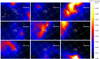 |
Fig. 6. Extinction maps at λ = 541.7 nm from Edenhofer et al. (2024) in the direction of GRB 221009A, integrated in the following distance intervals: 157–225 pc (top-left panel), 243–311 pc (top-central panel), 357–425 pc (top-right panel), 421–493 pc (center-left panel), 503–574 pc (central panel), 357-425 pc (center-right panel), 652–717 pc (bottom-left panel), 683–754 pc (bottom-central panel), and 740–812 pc (bottom-right panel). The regions covered by the two sectors studied in this work are highlighted in white in each panel. The green grid indicates the Galactic coordinates in degrees. |
4.3. Comparison with the Green map
The Green et al. (2019) map combines stellar photometry from Gaia Data Release 2 (DR2), Pan-STARRS 1, and 2MASS to provide extinction estimates with Gaia DR2 parallaxes. The map provides cumulative extinction across sight lines in 120 logarithmically spaced distance bins ranging from 63 pc to 63 kpc. In the direction of GRB 221009A, extinction can be measured for stars at distances from ∼0.3 to ∼5 kpc, extending well beyond the volume covered by the Lallement et al. (2022) and Edenhofer et al. (2024) maps. The angular resolution varies between 3.4′ and 13.7′, depending on the region of the sky. This map is also publicly available via the Python package DUSTMAPS. It provides extinction values in arbitrary units, which we converted to Av using the conversion formula outlined in Green et al. (2019, see their Table 1 and Eq. (30)).
We compared our pseudo-distance distributions in the two sectors with those from Green et al. (2019), using the Av − NH conversion factor from T23. The comparison was carried out by extracting the Green et al. (2019) maps of Sector 1 (brown in Fig. 7) and Sector 2 (green in Fig. 7) from the same directions chosen for the Edenhofer et al. (2024) maps in Sect. 4.2. As shown in the left panel of Fig. 7, the pseudo-distance distributions (Sector 1 in black and Sector 2 in blue) yield a total NH along the line of sight within our Galaxy that is lower than the values found by Green et al. (2019) in the same sector. As already discussed in Sect. 4.2, this discrepancy could result from our choice of the GRB fluence, which, as explained in T23, is affected by large systematic uncertainties. For example, by decreasing the GRB fluence by a factor of 1.35, the cumulative NH obtained from X-ray dust scattering in Sector 1 matches that of the Green map in the same sector at ∼700 pc and at 5 kpc and the one of Edenhofer et al. (2024, reported in orange in Fig. 7) from 700 pc to 1 kpc. The total value of NH, sca 1 = (6.07 ± 0.05)×1021 cm−2 is consistent with the average value provided by the Planck Collaboration XI (2014) 2D map in Sector 1: NH = (6.3 ± 0.4)×1021 cm−2. The absorption value in the host galaxy found with this revised fluence is NH, z = 0.151 = (3.7 ± 0.3)×1021 cm−2. The difference ΔNH = 2.48 × 1021 cm−2 between the values derived by Green et al. (2019) for the two sectors at 5 kpc (the farthest distance at which Green et al. 2019 can estimate stellar extinction) is consistent with the difference in X-ray absorption in the two sectors derived from the spectral analysis described in Sect. 3.2 (ΔNH, abs = 2.4 ± 0.3 × 1021 cm−2). On the contrary, even assuming the reduced fluence, the excess of dust in Sector 2 derived from X-ray scattering is significantly smaller: ΔNH, sca = (1.63 ± 0.07)×1021 cm−2. To achieve a compatible value, the dust content within 300 pc in Sector 2 should be ∼1.6 times greater than that in Sector 1 at the same distance. Finally, we note that, as the X-ray absorption is primarily due to gas along the line of sight, these values could also be reconciled by assuming a different dust-to-gas ratio (see, e.g., Zhu et al. 2017).
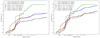 |
Fig. 7. Cumulative hydrogen column densities obtained from X-ray dust scattering for Sector 1 (black) and Sector 2 (blue), calculated using either the best-fit fluence from T23 (left panel) or a factor of 1.35 smaller fluence (right panel). In both cases, the same dust distribution for distances < 300 pc were assumed for the two sectors. Both panels also show a comparison with the cumulative hydrogen column density derived from Green et al. (2019, brown for Sector 1 and green for Sector 2) and from Edenhofer et al. (2024, orange for Sector 1 and red for Sector 2). A conversion factor between NH and Av equal to 1.9 × 1021 cm−2 mag−1 was used. |
4.4. Impact on GRB 221009A properties
Our last estimate of the X-ray absorption in the host galaxy, NH, z = 0.151 = (3.7 ± 0.3)×1021 cm−2, is significantly smaller than the value obtained by Williams et al. (2023) from the analysis of the afterglow X-ray spectrum, NH, z = 0.151 = (1.4 ± 0.4)×1022 cm−2. This difference can be explained by the smaller value assumed by Williams et al. (2023) for the Galactic absorption (NH, Gal = 5.38 × 1021 cm−2), derived from a NH map with poor angular resolution (Willingale et al. 2013). As already noted in T23, the NH inferred from Planck data (NH, Gal ≃ 9 × 1021 cm−2; Planck Collaboration XI 2014) indicates a significantly greater absorption in our Galaxy at the afterglow position.
In the analysis of the multiwavelength afterglow reported by Kann et al. (2023), the impact of multiple values for the Galactic extinction, ranging from 0 to Av = 5.2 mag (corresponding to no additional extinction in the host galaxy), was explored. Fulton et al. (2023) determined that in order to align the optical and X-ray fluxes observed 1–2 days after the burst, an additional extinction of Av = 1.5 mag (NH = 2.85 × 1021 cm−2 using a conversion factor NH/Av = 1.9 × 1021 cm−2 mag−1; T23) is required. This excess is likely due to the contribution of the ISM in the host galaxy and it is only slightly smaller than our estimate, which corresponds to NH = (3.5 ± 0.3)×1021 cm−2, if the correction due to the host galaxy redshift is not applied. Actually, Fulton et al. (2023) observed that this additional extinction decreased to 1.0 mag and 0.8 mag 2–3 days and 4–5 days after the GRB, respectively. The slightly larger X-ray absorption that we derive from the spectral analysis of the dust-scattered prompt GRB emission might therefore be part of this decreasing trend. A similar variability with time has been observed in other GRBs, such as GRB 190114C, and attributed to the photo-ionization of the surrounding ISM (Campana et al. 2021).
The best estimate of the X-ray fluence of GRB 221009A in the soft X-ray range given in T23 (2.6 × 10⁻³ erg cm−2) is approximately an order of magnitude larger than the value obtained by extrapolating to the same energy range the GRB spectrum observed at higher energies (Frederiks et al. 2023; An et al. 2023; Burns et al. 2023). This estimate was derived assuming the amount of dust in the cloud at 0.73 kpc as determined by Lallement et al. (2022), which, as discussed in Sect. 4.1, lacks adequate angular resolution. Decreasing the fluence by a factor or 1.9 or 1.35, as suggested by the spatially resolved analysis reported in Sects. 3.2 and 4.3, respectively, would only partially reduce the magnitude of the soft excess found in T23, which would still be a few times brighter than the extrapolation of the prompt GRB emission estimated from hard X-ray data.
The sector analysis reported here and the adoption of different extinction maps allow us to better control systematic effects, but our results are still based on a single dust model (BARE-GR-B) and a specific relation between hydrogen column density and optical extinction (NH = 1.9 × 10²¹ Av cm−2 mag−1; T23). Even if the BARE-GR-B model is the best one describing the dust responsible for the X-ray rings observed around GRB 221009A, T23 have shown that other dust models provide similarly good fits to the ring spectra (e.g., COMP-GR-B from Zubko et al. 2004 or the Draine 2003 model). In these cases, we obtain a GRB fluence that can be different by up to a factor of 1.5. Additionally, the NH/Av relationship is also subject to systematic uncertainties, as demonstrated by the scatter in previous measurements across various sky regions and astrophysical objects, which range from 1.0 × 10²¹ to 2.8 × 1021 cm−2 mag−1 (Zhu et al. 2017). Finally, although the spatially resolved spectral analysis of the X-ray rings reported in Appendix A suggests that all the dust clouds are formed by dust grains with the same properties, we cannot exclude the existence of different dust populations depending on the local environment.
5. Conclusion
We have presented a detailed analysis of the dust-scattered X-ray emission from GRB 221009A observed by XMM-Newton and Swift/XRT. The main aim of this analysis, supported by a comparison with recently published 3D extinction maps, was to constrain the properties of the ISM in the GRB direction, both in our Galaxy and in the host galaxy. In particular, we generated a 3D map of the Galactic dust distribution in a ∼0.5° wide region centered at the position of the GRB with a better resolution than previous studies, both in the plane of the sky (a few arcminutes) and along the radial direction (approximately 1 pc for distances D < 1 kpc and 100 pc for D > 10 kpc). Although this map covers a very small sky region, the dust cloud distances are directly measured throughout the whole Galaxy using a geometrical method, in analogy with parallaxes for stars, and can therefore be used to calibrate other maps based on indirect or model-dependent distance measurements.
In addition, the spectral analysis of the brightest X-ray rings revealed considerable variability in the hydrogen column density of the total absorbing matter across the FOV, which, coupled to the correlated intensity variability of the dust-scattered radiation, allowed us to separate Galactic absorption from the host galaxy contribution. Such a measurement is crucial not only for characterizing the GRB local environment and its time evolution induced by the burst radiation, but also for constraining the intrinsic luminosity of a possibly associated supernova (see, e.g., Shrestha et al. 2023).
Finally, this work refined the soft X-ray fluence estimate from T23 (2.6 × 10⁻³ erg cm−2), reducing it by a factor of at least 1.35. However, the revised values, based on the comparison of our modeling of the dust-scattering rings with three different 3D extinction maps, are not small enough to rule out the soft excess in the prompt X-ray emission found in the previous work.
For pn data: #XMMEA_EP& & (FLAG==0)& & (PATTERN< =4) and for MOS: #XMMEA_EM& & (PATTERN< =12).
Since we are interested only in the spectral shape to constrain the absorption, we can ignore the brightness of the X-ray rings.
The map is publicly available on the EXPLORE website: https://explore-platform.eu.
The EPIC CCD cameras on board XMM-Newton are equipped with a filter wheel system and 6 different filter setups, including a closed position, in which the sky is blocked by a ∼ 1 mm thick layer of aluminum. The FWC exposures, which are dominated by the instrumental background, are typically used to model and subtract the internal instrumental background of the XMM-Newton EPIC CCD cameras.
Acknowledgments
This publication was produced while B.V. attending the PhD program in Space Science and Technology at the University of Trento, Cycle XXXVIII, with the support of a scholarship financed by the Ministerial Decree no. 351 of 9th April 2022, based on the NRRP – funded by the European Union – NextGenerationEU – Mission 4 “Education and Research”, Component 1 “Enhancement of the offer of educational services: from nurseries to universities” – Investment 4.1 “Extension of the number of research doctorates and innovative doctorates for public administration and cultural heritage”. AB acknowledges the financial support of INAF through the initiative “IAF Astronomy Fellowships in Italy” (grant name MEGASKAT). SC acknowledge support from ASI under contract ASI/INAF I/004/11/6.
References
- An, Z.-H., Antier, S., Bi, X.-Z., et al. 2023, arXiv e-prints [arXiv:2303.01203] [Google Scholar]
- Arnaud, K. A. 1996, in Astronomical Data Analysis Software and Systems V, eds. G. H. Jacoby, & J. Barnes, ASP Conf. Ser., 101, 17 [NASA ADS] [Google Scholar]
- Bohlin, R. C., Savage, B. D., & Drake, J. F. 1978, ApJ, 224, 132 [Google Scholar]
- Burns, E., Svinkin, D., Fenimore, E., et al. 2023, ApJ, 946, L31 [NASA ADS] [CrossRef] [Google Scholar]
- Burrows, D. N., Hill, J. E., Nousek, J. A., et al. 2005, Space Sci. Rev., 120, 165 [Google Scholar]
- Campana, S., Lazzati, D., Perna, R., Grazia Bernardini, M., & Nava, L. 2021, A&A, 649, A135 [NASA ADS] [CrossRef] [EDP Sciences] [Google Scholar]
- Draine, B. T. 2003, ApJ, 598, 1026 [Google Scholar]
- Draine, B. T., & Allaf-Akbari, K. 2006, ApJ, 652, 1318 [Google Scholar]
- Edenhofer, G., Zucker, C., Frank, P., et al. 2024, A&A, 685, A82 [NASA ADS] [CrossRef] [EDP Sciences] [Google Scholar]
- Frederiks, D., Svinkin, D., Lysenko, A. L., et al. 2023, ApJ, 949, L7 [NASA ADS] [CrossRef] [Google Scholar]
- Fulton, M. D., Smartt, S. J., Rhodes, L., et al. 2023, ApJ, 946, L22 [NASA ADS] [CrossRef] [Google Scholar]
- Gabriel, C., Denby, M., Fyfe, D. J., et al. 2004, in Astronomical Data Analysis Software and Systems (ADASS) XIII, eds. F. Ochsenbein, M. G. Allen, & D. Egret, ASP Conf. Ser., 314, 759 [NASA ADS] [Google Scholar]
- Gastaldello, F., Marelli, M., Molendi, S., et al. 2022, ApJ, 928, 168 [NASA ADS] [CrossRef] [Google Scholar]
- Gehrels, N., Chincarini, G., Giommi, P., et al. 2004, ApJ, 611, 1005 [Google Scholar]
- Green, G. 2018, The Journal of Open Source Software, 3, 695 [Google Scholar]
- Green, G. M., Schlafly, E., Zucker, C., Speagle, J. S., & Finkbeiner, D. 2019, ApJ, 887, 93 [NASA ADS] [CrossRef] [Google Scholar]
- Heinz, S., Corrales, L., Smith, R., et al. 2016, ApJ, 825, 15 [NASA ADS] [CrossRef] [Google Scholar]
- Johansen, A., & Lambrechts, M. 2017, Annual Review of Earth and Planetary Sciences, 45, 359 [CrossRef] [Google Scholar]
- Kann, D. A., Agayeva, S., Aivazyan, V., et al. 2023, ApJ, 948, L12 [NASA ADS] [CrossRef] [Google Scholar]
- Lallement, R., Vergely, J. L., Babusiaux, C., & Cox, N. L. J. 2022, A&A, 661, A147 [NASA ADS] [CrossRef] [EDP Sciences] [Google Scholar]
- Mie, G. 1908, Annalen der Physik, 330, 377 [CrossRef] [Google Scholar]
- Miralda-Escudé, J. 1999, ApJ, 512, 21 [Google Scholar]
- Pintore, F., Tiengo, A., Mereghetti, S., et al. 2017, MNRAS, 472, 1465 [NASA ADS] [CrossRef] [Google Scholar]
- Planck Collaboration XI. 2014, A&A, 571, A11 [NASA ADS] [CrossRef] [EDP Sciences] [Google Scholar]
- Predehl, P., & Schmitt, J. H. M. M. 1995, A&A, 293, 889 [NASA ADS] [Google Scholar]
- Psaradaki, I., Costantini, E., Rogantini, D., et al. 2023, A&A, 670, A30 [NASA ADS] [CrossRef] [EDP Sciences] [Google Scholar]
- Schlafly, E. F., & Finkbeiner, D. P. 2011, ApJ, 737, 103 [Google Scholar]
- Schneider, R., Ferrara, A., Natarajan, P., & Omukai, K. 2002, ApJ, 571, 30 [CrossRef] [Google Scholar]
- Shrestha, M., Sand, D. J., Alexander, K. D., et al. 2023, ApJ, 946, L25 [NASA ADS] [CrossRef] [Google Scholar]
- Šiljeg, B., Bošnjak, Ž., Jelić, V., et al. 2023, MNRAS, 526, 2605 [Google Scholar]
- Smith, R. K. 2008, ApJ, 681, 343 [Google Scholar]
- Strüder, L., Briel, U., Dennerl, K., et al. 2001, A&A, 365, L18 [Google Scholar]
- Tiengo, A., & Mereghetti, S. 2006, A&A, 449, 203 [NASA ADS] [CrossRef] [EDP Sciences] [Google Scholar]
- Tiengo, A., Vianello, G., Esposito, P., et al. 2010, ApJ, 710, 227 [Google Scholar]
- Tiengo, A., Pintore, F., Vaia, B., et al. 2023, ApJ, 946, L30 [NASA ADS] [CrossRef] [Google Scholar]
- Turner, M. J. L., Abbey, A., Arnaud, M., et al. 2001, A&A, 365, L27 [CrossRef] [EDP Sciences] [Google Scholar]
- Vasilopoulos, G., Karavola, D., Stathopoulos, S. I., & Petropoulou, M. 2023, MNRAS, 521, 1590 [NASA ADS] [Google Scholar]
- Vaughan, S., Willingale, R., O’Brien, P. T., et al. 2004, ApJ, 603, L5 [Google Scholar]
- Williams, M. A., Kennea, J. A., Dichiara, S., et al. 2023, ApJL, 946, L24 [CrossRef] [Google Scholar]
- Willingale, R., Starling, R. L. C., Beardmore, A. P., Tanvir, N. R., & O’Brien, P. T. 2013, MNRAS, 431, 394 [Google Scholar]
- Zhang, X., Green, G. M., & Rix, H.-W. 2023, MNRAS, 524, 1855 [NASA ADS] [CrossRef] [Google Scholar]
- Zhao, G., & Shen, R.-F. 2024, ApJ, 970, 124 [NASA ADS] [Google Scholar]
- Zhu, H., Tian, W., Li, A., & Zhang, M. 2017, MNRAS, 471, 3494 [NASA ADS] [CrossRef] [Google Scholar]
- Zubko, V., Dwek, E., & Arendt, R. G. 2004, ApJS, 152, 211 [NASA ADS] [CrossRef] [Google Scholar]
Appendix A: Azimuthal variability of X-ray absorption
To optimize the selection of azimuthal sectors for mapping the Galactic dust in the directions around the GRB 221009A position, a spectral analysis of annular sectors with similar numbers of counts was performed to evaluate the possible variation of X-ray absorption. The MOS2 FOV in Obs2 was divided into seven concentric annuli (labeled rings A through G) with adjacent scattering rings grouped together to form regions containing at least 8000 counts (Fig.A.1). Each ring was then further subdivided into eight sectors, ensuring that all sectors within the same ring had about the same number of counts (>1000, to maintain sufficient statistics). The background spectra were obtained from the same region but extracted from the late time observation made with XMM-Newton on November 11. The spectra of each annular sector were simultaneously fit using the XSPEC model already adopted in T23: CONSTANT × zTBabs × TBabs × RINGSCAT × EGPWRLW. In this model, RINGSCAT takes into consideration the product ΔNH σθ1, 2(E) in Eq. 3 and the prompt GRB spectrum is modeled as a power law (PEGPWRLW) modified by absorption in both our Galaxy (TBABS) and the host galaxy (ZTBABS). The model RINGSCAT is based on the exact Mie calculation of the scattering cross section on spherical grains (Mie 1908), with composition and size distribution according to the BARE-GR-B model (Zubko et al. 2004). In this dust model, which provides the best-fit to the spectra of the 19 X-ray rings analyzed in T23, the grains are bare (uncoated), composed of graphite, silicate and polycyclic aromatic hydrocarbons, and B star abundances are assumed (Zubko et al. 2004). All the parameters were fixed to the best-fit values found in T23, except for the Galactic absorption and the overall normalization (CONSTANT). An acceptable fit (χ2/dof = 2207/2177; nhp = 32%) was obtained, which means that the angular dependence of the scattering cross section (modeled by the RINGSCAT spectral component) and a spatially variable Galactic absorption can fully explain the spectral variability detected across the MOS2 FOV. The best-fit Galactic absorption hydrogen column densities derived for each spectrum are shown in Fig. A.2. Ring F, which contains the X-ray radiation scattered by dust at ∼700 pc, displays significant azimuthal variability, with a prominent absorption excess in sectors F3 and F4, which range from 94° to 180°. The level of X-ray absorption in the other sectors of this ring, NH = 0.726 ± 0.018, is compatible with the constant values derived for the other rings with radii larger than ∼3′. For Ring A, we instead found a lower column density, but, at such small angles, both the subtraction of the X-ray afterglow and the calculation of the scattering cross section are affected by larger systematic uncertainties.
 |
Fig. A.1. Annular sectors in which we performed the spectral analysis to evaluate the variation in X-ray absorption. The inner and outer radii for each ring are: Ring A (2′-3.37′), Ring B (3.37′-4.88′), Ring C (4.88′-5.62′), Ring D (5.62′-7.27′), Ring E (7.27′-10.85′), Ring F (10.85′-12.1′), and Ring G (12.1′-14.2′). Each ring is divided into eight sectors containing the same number of counts. |
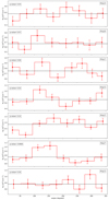 |
Fig. A.2. X-ray absorption for the seven rings derived from the spectral analysis using the model CONSTANT × zTBabs × TBabs × RINGSCAT × PEGPWRLW. Each sector within the same region is fit with a constant, yielding acceptable fits (p-value displayed in the upper left of each plot) for all rings except for Ring F. |
Appendix B: Background subtraction in pseudo-distance distributions
The subtraction of the contribution of events not produced by X-ray dust scattering to the pseudo-distance distribution is crucial to avoid overestimating the quantity of dust in our Galaxy. To analyze the Swift/XRT observations, we implemented a double background-subtraction technique to isolate the emission from the rings by removing contributions from both the sky and instrumental background and the GRB afterglow. First, we constructed a pseudo-distance distribution for each sector from late-time observations (Obs IDs from 01126853076 to 01126853084). These background distributions were generated by randomizing the time within the range of the Swift/XRT observations of the GRB during which the rings were visible and by measuring the angular distance from the GRB in sky coordinates.
To further remove the afterglow, we used a second set of observations taken about 15 days after the burst (Obs IDs from 01126853023 to 01126853027). By this time, the afterglow was still bright, but the flux of the X-ray rings was below the detection threshold. The pseudo-distance distribution for the afterglow in each sector was produced as for the late time observations, which, in turn, were used to obtain a background-subtracted afterglow distribution. Such distributions were then enhanced by a factor corresponding to the ratio of the average afterglow flux in the 0.3 - 5 keV energy band measured during the observations from October 10 to 13 (when the rings were detected) and from October 25 to 29 (from which we extracted the pseudo-distance distribution of the afterglow). To obtain the net contribution from the X-ray dust scattering halo, we therefore subtracted from the original pseudo-distance distributions of the two sectors both these afterglow distributions and those obtained for the background at late times.
In the two XMM-Newton observations, we did not utilize late-time observations as background, due to the residual contamination by X-ray dust scattering. Instead, we subtracted both the sky background and the afterglow contribution using a single observation of a different target (RBS 315; see Sect. 2 for details).
For the first XMM-Newton observation (Obs1), the subtraction was straightforward, involving a direct subtraction between the two pseudo-distance distributions, where angular distances were calculated in detector coordinates and the arrival times of the events in the background observation were randomly attributed in the time interval covered by Obs1. On the contrary, the subtraction in the second XMM-Newton observation (Obs2) was complicated by the presence of an anomalous electronic noise in some MOS2 CCDs. Specifically, the ratio between the counts in individual CCDs and the total counts in the 5-10 keV band (where the X-ray rings are not detectable) showed an excess with respect to filter wheel closed (FWC) exposures4. For Obs1 and the background observation, instead, the count ratios of every CCD were consistent with those observed in the FWC exposures.
To account for this anomalous background in Obs2, we rescaled the background pseudo-distance distribution of each CCD before performing the subtraction. The rescaling factor was the ratio between the 5-10 keV counts in Obs2 and those in the background observation for each CCD.
Appendix C: Calculation of the conversion factors for pseudo-distance distributions
To compute the conversion factors f(θ, t), which allow us to transform the pseudo-distance distributions C(D) into the equivalent hydrogen column density of the dust ΔNH(D), we divided the two sectors into annular regions, with a width of 30″, ranging from 2′ to 12′ and extracted the corresponding spectra. For each spectrum, a specific response matrix was generated. Using XSPEC (Arnaud 1996), we calculated the expected number of detected counts in each spectrum C(D) for a fixed amount of dust, calculating the distance D from Eq. 6, where t is the time elapsed between the GRB and the middle of the observation and θ is the average radius of the spectral extraction region. For the scattered emission, we adopted the model reported in T23 and briefly described in Appendix A: CONSTANT × zTBabs × TBabs × ringscat × pegpwrlw. In this case, the CONSTANT is the inverse of the exposure time, adjusted by the ratio of the sector’s angular dimension to the full circle (105° /360°) and the amount of dust in RINGSCAT is fixed to ΔNH = 1021cm−2. All the other spectral parameters, including the GRB fluence of FGRB = 2.6 × 10⁻³ erg cm−2, are fixed to the best-fit values reported in T23. The conversion factor f(θ, t) for each dataset, in units of 1021cm−2, is therefore the inverse of the number of expected counts in the 0.7–4 keV energy band, from which the pseudo-distance distributions were extracted.
All Tables
All Figures
|
Fig. 1. Combined XMM-Newton X-ray observations of GRB 221009A, with the two sectors used for our analysis highlighted. |
| In the text | |
|
Fig. 2. Left: differential hydrogen column density in Sector 1. The Swift-XRT data are in green, the data obtained with the first XMM-Newton observation in black, and the data obtained with the second XMM-Newton observation in red. Right: Differential hydrogen column density in Sector 2. The data obtained with the first XMM-Newton observation are in black, and the data obtained with the second XMM-Newton observation in red. The blue arrows highlight the four main peaks observed by both XMM-Newton and Swift. |
| In the text | |
|
Fig. 3. Hydrogen column density obtained by integrating the pseudo-distance distribution at the four main peaks in Fig. 2 (highlighted with blue arrows), centered at 406.3 pc (leftmost panel), 475.2 pc (center-left panel), 553.6 pc (center-right panel), and ∼700 pc (rightmost panel). The inset of the last panel shows the two clouds around 700 pc as separate values: the circles refer to the peak at 695.4 pc (Swift-XRT in blue, XMM-Newton in brown for Obs1, and pink for Obs2), and the squares to the peak centered at 728.6 pc (Swift-XRT in green, XMM-Newton in black for Obs1, and red for Obs2). In all the other panels the values from Swift-XRT observations are shown in green, and from XMM-Newton observations in black (Obs1) and red (Obs2). |
| In the text | |
|
Fig. 4. Cumulative hydrogen column density in our Galaxy for Sector 1 (solid black lines) and Sector 2 (solid blue lines) derived from ring emission under different assumptions: GRB fluence from T23 (left panel); 1.9 times lower fluence than in T23 (middle panel); GRB fluence from T23 and 2.6 times more dust in Sector 2 than in Sector 1 within 300 pc (right panel). In the first two panels, the same dust concentration is assumed for both sectors at distances < 300 pc. The dashed lines (black for Sector 1, blue for Sector 2) indicate the total hydrogen column density, including contributions from both our Galaxy and the host galaxy, measured from the absorption inferred from X-ray spectral fitting. |
| In the text | |
|
Fig. 5. Differential hydrogen column density derived from X-ray dust scattering for Sector 1 (black) and Sector 2 (blue), compared to 3D optical extinction maps. Left: Values derived by Lallement et al. (2022), displayed in pink. Right: Differential hydrogen column density from Edenhofer et al. (2024) for Sector 1 (in orange) and Sector 2 (in red). A conversion factor of 1.9 × 1021 cm−2 mag−1 between NH and Av was used. |
| In the text | |
|
Fig. 6. Extinction maps at λ = 541.7 nm from Edenhofer et al. (2024) in the direction of GRB 221009A, integrated in the following distance intervals: 157–225 pc (top-left panel), 243–311 pc (top-central panel), 357–425 pc (top-right panel), 421–493 pc (center-left panel), 503–574 pc (central panel), 357-425 pc (center-right panel), 652–717 pc (bottom-left panel), 683–754 pc (bottom-central panel), and 740–812 pc (bottom-right panel). The regions covered by the two sectors studied in this work are highlighted in white in each panel. The green grid indicates the Galactic coordinates in degrees. |
| In the text | |
|
Fig. 7. Cumulative hydrogen column densities obtained from X-ray dust scattering for Sector 1 (black) and Sector 2 (blue), calculated using either the best-fit fluence from T23 (left panel) or a factor of 1.35 smaller fluence (right panel). In both cases, the same dust distribution for distances < 300 pc were assumed for the two sectors. Both panels also show a comparison with the cumulative hydrogen column density derived from Green et al. (2019, brown for Sector 1 and green for Sector 2) and from Edenhofer et al. (2024, orange for Sector 1 and red for Sector 2). A conversion factor between NH and Av equal to 1.9 × 1021 cm−2 mag−1 was used. |
| In the text | |
|
Fig. A.1. Annular sectors in which we performed the spectral analysis to evaluate the variation in X-ray absorption. The inner and outer radii for each ring are: Ring A (2′-3.37′), Ring B (3.37′-4.88′), Ring C (4.88′-5.62′), Ring D (5.62′-7.27′), Ring E (7.27′-10.85′), Ring F (10.85′-12.1′), and Ring G (12.1′-14.2′). Each ring is divided into eight sectors containing the same number of counts. |
| In the text | |
|
Fig. A.2. X-ray absorption for the seven rings derived from the spectral analysis using the model CONSTANT × zTBabs × TBabs × RINGSCAT × PEGPWRLW. Each sector within the same region is fit with a constant, yielding acceptable fits (p-value displayed in the upper left of each plot) for all rings except for Ring F. |
| In the text | |
Current usage metrics show cumulative count of Article Views (full-text article views including HTML views, PDF and ePub downloads, according to the available data) and Abstracts Views on Vision4Press platform.
Data correspond to usage on the plateform after 2015. The current usage metrics is available 48-96 hours after online publication and is updated daily on week days.
Initial download of the metrics may take a while.