| Issue |
A&A
Volume 696, April 2025
|
|
|---|---|---|
| Article Number | A171 | |
| Number of page(s) | 13 | |
| Section | Interstellar and circumstellar matter | |
| DOI | https://doi.org/10.1051/0004-6361/202452579 | |
| Published online | 21 April 2025 | |
Hunting pre-stellar cores with APEX: Corona Australis 151, the densest pre-stellar core or the youngest protostar?
1
European Southern Observatory,
Karl-Schwarzschild-Strasse 2,
85748
Garching,
Germany
2
Max-Planck-Institut für Extraterrestrische Physik,
Giessenbachstrasse 1,
85748
Garching,
Germany
3
Department of Physics, University of Helsinki,
PO Box 64,
00014
Helsinki,
Finland
4
National Astronomical Observatory of Japan,
Osawa 2-21-1,
Mitaka, Tokyo
181-8588,
Japan
5
Max-Planck-Institut für Radioastronomie,
Auf dem Hügel, 69,
53121
Bonn,
Germany
★ Corresponding author; This email address is being protected from spambots. You need JavaScript enabled to view it.
Received:
11
October
2024
Accepted:
19
February
2025
Abstract
Context. Pre-stellar cores are the birthplaces of Sun-like stars and represent the initial conditions for the assembly of protoplanetary systems. Due to their short lifespans, they are rare. As part of recent efforts to increase the number of such sources identified in the solar neighbourhood, we have selected a sample of 40 starless cores from the publicly available core catalogues of the Herschel Gould Belt survey. In this work, we focus on a source that stands out for its high central density: Corona Australis 151.
Aims. We used molecular lines that trace dense gas (n ≳ 106 cm−3) to confirm the exceptionally high density of this object, study its physical structure, and understand its evolutionary stage.
Methods. We detected the N2H+ 3 − 2 and 5 − 4 transitions and the N2D+ 3 − 2, 4 − 3, and 6 – 5 lines with the Atacama Pathfinder EXperiment (APEX) telescope. We used the Herschel continuum data to infer a spherically symmetric model of the core’s density and temperature. This was used as input to perform a non-local-thermodynamic-equilibrium radiative transfer to fit the five observed lines.
Results. Our analysis confirms that this core is characterised by very high densities (a few × 107 cm−3 at the centre) and cold temperatures (8 − 12 K). We inferred a high deuteration level of N2D+/N2H+ = 0.50, indicative of an advanced evolutionary stage. In the large bandwidth covered by the APEX data, we detected several other deuterated species, including CHD2OH, D2CO, and ND3. We also detected multiple sulphurated species that present broader lines with signs of high-velocity wings.
Conclusions. High-angular resolution observations will be necessary to unveil the evolutionary stage of Cra 151. The detection of a compact emission at 70 μm does not exclude that the source is a first hydrostatic core or in a very early stage of the protostellar phase. The observation of high-velocity wings and the fact that the linewidths of N2H+ and N2D+ become larger with increasing frequency can be interpreted as either an indication of supersonic infall motions developing in the central parts of a very evolved pre-stellar core or the signature of outflows from a very low luminosity object.
Key words: stars: formation / ISM: clouds / ISM: molecules / radio lines: ISM / ISM: individual objects: Corona Australis 151
© The Authors 2025
 Open Access article, published by EDP Sciences, under the terms of the Creative Commons Attribution License (https://creativecommons.org/licenses/by/4.0), which permits unrestricted use, distribution, and reproduction in any medium, provided the original work is properly cited.
This article is published in open access under the Subscribe to Open model. This email address is being protected from spambots. You need JavaScript enabled to view it. to support open access publication.
1 Introduction
Pre-stellar cores are the preferred location for star formation. These dense and cold fragments of molecular clouds represent the initial conditions for the assembly of stellar systems, and their study is therefore crucial to understanding the subsequent planetary formation. These objects, however, are rare due to their short lifetimes before the gravitational collapse. Embedded in the Taurus molecular cloud, L1544 represents a prototypical example of a pre-stellar core. Recent observations with the Atacama Large Millimeter and sub-millimeter Array (ALMA; Caselli et al. 2019, 2022) have shown the existence of a high-density “kernel” at its centre (size: ≲ 2000 au, temperature 6 K, density n < 107 cm−3), which is in agreement with the predictions of theoretical works focusing on the dynamical evolution of contracting magnetised clouds (e.g. Galli & Shu 1993).
In recent observational efforts, we have sought to expand the catalogue of known pre-stellar cores in order to increase our understanding of their physical and chemical properties statistically. We have identified a sample based on data from the Herschel Gould Belt Survey Archive (HGBS1; André et al. 2010), and we have targeted the sample with single-dish observations of high frequency (230 − 460 GHz) lines of N2H+ and N2D+. The whole sample, which comprises the densest starless cores identified in the HGBS within 200 pc from the Solar System, is presented and described in Caselli et al. (in prep.). The high-J transitions of N2H+ and N2D+ can be used to confirm the high central density due to their high critical densities (ncrit ≳ 106 cm−3). Furthermore, the deuteration level of diazenylium RD = N(N2D+)/N(N2H+) is a well-known evolutionary indicator for the pre-stellar phase (see Crapsi et al. 2005). These species are formed from molecular nitrogen, which chemically is a late-type molecule (see e.g. Hily-Blant et al. 2010). Furthermore, the deuteration process is efficient at advanced evolutionary stages, as it is enhanced by low temperatures and high CO depletion factors (Dalgarno & Lepp 1984; see also the review from Ceccarelli et al. 2014). Using the low- J transitions of N2H+ and N2D+, Crapsi et al. (2005) found that a high deuteration level (RD > 0.1) is a sign of a centrally concentrated core with a high degree of CO depletion.
From the sample, we identified the objects where the high rotational transitions (in particular N2D+ 6 − 5 and N2H+ 5 − 4) have been successfully detected in order to study them in detail. The present work focuses on the core found in the CrA-E region identified as Corona Australis 151 (hereafter, CrA 151) in the HGBS core catalogue of Bresnahan et al. (2018). A companion work analyses the core Ophiuchus 464, also known as IRAS 16293E (Spezzano et al. 2025).
The Corona Australis molecular cloud is a well-studied low-mass star-forming region in the Southern Hemisphere. Its morphology has been studied in detail using Herschel data as part of the HGBS survey (Bresnahan et al. 2018). Its shape resembles a cometary head in the western part, and there are two filamentary structures stretching towards the east. Star formation is particularly active in the western end, which hosts the so-called Coronet cluster. This region is known to host several young stellar objects (YSOs) at distinct evolutionary stages (see Chini et al. 2003; Sicilia-Aguilar et al. 2013). Star formation appears less active in the rest of the cloud. The most recent distance estimate for Corona Australis is d = 150 pc, based on Gaia data (Galli et al. 2020). We adopt this value throughout this work.
The core CrA 151 sits in the northern filament of Bresnahan et al. (2018, region CrA-E) at about 5 pc east of the Coronet cluster. It corresponds to Cloud 42 of Sandqvist & Lindroos (1976). The region contains ≈20 M⊙ of total mass and one robust prestellar core candidate (CrA 151 itself). No young star, disc, or YSO is known within the core boundaries, according to the census reported in Esplin & Luhman (2022), which is based on proper motions measured from multi-epoch IR imaging from the Spitzer Space Telescope and Magellan Observatory and positions in the colour-magnitude diagram measured with Gaia, 2MASS, VISTA VHS, WISE, Spitzer, and Magellan. However, Bresnahan et al. (2018) detected a point source at 70 μm towards Cra 151 with Herschel/PACS. Whilst emission at 70 μm is not conclusive proof of the presence of a central heating source and the detection is at the 4σ level, it might indicate the presence of a very low luminosity object (VeLLO; di Francesco et al. 2007; Tomida et al. 2010), which could be a very young low-mass protostar or a first hydrostatic core (FHSC; Larson 1969). Hardegree-Ullman et al. (2013) studied the region using C18O and N2H+ 1 − 0 observations from the Swedish ESO Submillimeter Telescope (SEST). The authors modelled the density profile of the core with a Plummer-like solution and the available continuum data, and they found a central density higher than 106 cm−3. They ran chemical modelling to investigate the core’s chemistry and discovered evidence of strong CO depletion. N2H+, instead, appears to have a rather constant abundance of a few multiples of 10−10. However, their line observations had limited angular resolution (∼ 50′′), and as the observations were targeting the low-J transitions of two abundant species, they were more sensitive to more extended regions within the core than our observations (see below).
This work is organised as follows. Section 2 describes the observational data. The obtained spectra and subsequent analysis are presented in Sect. 3, where first we develop the physical model of the source (Sect. 3.2) and then we present the radiative transfer modelling of the spectroscopic lines (Sect. 3.3). Section 3.4 describes other species detected in the frequency coverage of the observations. We discuss the results of the analysis in Sect. 4. Section 5 contains a summary and final remarks of this work.
2 Observations
The data of the diazenylium lines analysed in this work were collected with the Atacama Pathfinder EXperiment (APEX; Güsten et al. 2006) telescope as part of the large core sample described in Caselli et al. (in prep.). We refer to that paper for an exhaustive description of the observational details. Here, we offer a summary for the particular case of CrA 151.
The data consist of single-pointing observations towards the core’s centre at coordinates RA(J2000) = 19h 10m 20s.17 and Dec(J2000) = −37∘08m 27s.0. Two tunings of the receiver SEPIA345 were used to cover the N2H+ 3 − 2 and N2D+ 4 − 3 transitions at 279.5 GHz and 308.4 GHz, respectively. These observations were performed in July and October 2022 (Proposal ID: O-0110.F-9310A-2022). The N2D+ 3 − 2 line was covered with the nFLASH230 receiver, whilst the N2D+ 6 − 5 and N2H+ 5 − 4 transitions were covered simultaneously with one tuning of nFLASH460 (we exploited the dual-channel capability of the nFLASH frontend; Klein et al. 2014). These observations were collected under project M-0110.F-9501C-2022 in September and November 2022.
In all cases, the observations were performed in ON-OFF position switching, with OFF coordinates △RA, ΔDec = (−300′′, 0) with respect to the core central coordinates. We used the FFTS backend, which allows for a spectral resolution of 64 kHz. This translates into a velocity resolution from ΔVch ∼ 0.08 km s−1 at 230 GHz to ∼ 0.04 km s−1 at 460 GHz.
We reduced the data using the CLASS package of the GILDAS software2. In particular, we subtracted baselines (usually a firstorder polynomial) in every scan and then averaged them. The intensity scale was converted into a main beam temperature TMB, assuming the forward efficiency Feff = 0.95 and computing the main-beam efficiency at each frequency according to ηMB = 1.00797 − 0.000857 * v(GHz). We obtained this relation fitting the tabulated data3. Relevant information on the targeted transitions and their observational parameters is given in Table 1, including the angular resolution (θMB) of the observations, which spans the range 13 − 26′′. At the distance of CrA 151, the linear resolution is 2000 − 4000 au.
3 Results and analysis
This section contains a description of the observed spectra of N2H+ and N2D+ and the analysis we performed to model them. It concludes with a discussion of the other lines that were covered by the APEX data.
3.1 Observed spectra
The plots of the observed N2H+ and N2D+ transitions are shown in Fig. 1. All the lines are robustly detected based on the sensitivities reached (rms reported in Table 1). The peak signal-to-noise ratios (S/Ns) span from S/N = 5(N2D+ 6 − 5) to S/N = 160 (N2D+ 3 − 2). We computed the critical densities of these transitions based on our own calculation from the collisional and Einstein rates of the pure rotational transitions (see Table 1). The values range from 7.4 × 10⁵ to 5.5 × 106 cm−3. Their detection with a single-dish facility at a resolution of 4000 au (at the lowest frequency) is indicative that high densities characterise a significant portion of the core. This point is discussed further in Sect. 3.2.
We fit the data assuming a constant excitation temperature for all the hyperfine components within each rotational transition using the HFS routine implemented in CLASS to obtain the kinematic parameters of the lines, namely, the local-standard-of-rest velocity (Vlsr) and the line full width half maximum (FWHM). The latter is the intrinsic linewidth and is not biased by opacity broadening. The obtained best-fit parameters are listed in the last two columns of Table 1, and the corresponding plots are shown in Appendix A. The Vlsr values obtained for N2H+ 5 − 4 and all the N2D+ transitions agree within 3σ around a weighted average of ⟨Vlsr⟩ = (5.6543 ± 0.0002) km s−1. The value for N2H+ 3 − 2 is lower: (5.612 ± 0.005) km s−1. The difference of ∼ 0.04 km s−1 is significant above the 5σ level. However, we highlight that this difference is smaller than the channel width at 1 mm. Furthermore, the N2H+ 3 − 2 transition shows a clear profile feature (the double peak seen in the central hyperfine group) that is not due to the hyperfine structure and cannot be reproduced by the HFS fitting routine (see Fig. A.1). This likely arises from gas motions within the core, possibly due to gravitational contraction, which results in double-peaked profiles with blue asymmetry in optically thick lines (Evans 1999). The total optical depth of this transition, estimated by CLASS, is τtot = 4.2 ± 0.3. The presence of this feature affects the determination of Vlsr for this line.
Concerning the linewidths, the transitions at ∼ 1 mm present narrow lines (FWHM ≈ 0.4 km s−1). The N2D+ 6 − 5 line appears broader even though its FWHM has large uncertainties due to the low S/N of the spectrum. On the other hand, the N2H+ 5 − 4 line is significantly broader (FWHM = 0.747 ± 0.011 km s−1).
Parameters of the targeted lines.
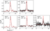 |
Fig. 1 Observations of the N2H+ and N2D+ transitions towards CrA 151 (black histograms) and synthetic spectra obtained with the MCMC approach applied to the non-LTE radiative transfer analysis (red histograms; see Sect. 3.3). |
3.2 Physical model of the source
To perform the non-LTE radiative transfer, we computed a spherically symmetric model of the source based on the available dust thermal emission data from Herschel. Figure 2 shows the three-colour RGB image obtained from the SPIRE and PACS wavelengths in the left panel, and the derived column density and dust temperature maps are shown in the remaining panels. The detailed procedure is described in Roy et al. (2014). Briefly, according to their Eq. (3), the product ρ(r) Bλ(Td) κλ, where Bλ is the Planck function at wavelength λ and κλ is the dust opacity at this wavelength, can be obtained from the inverse Abel transformation of the surface brightness gradient dIλ/dr as a function of the impact parameter. The density and temperature profiles were fit by determining the surface brightness gradient at four wavelengths. For the dust opacity, we assumed κ250 μm = 0.1 cm2 g−1 and a dust opacity index of β = 2.0 (Hildebrand 1983). We used the Herschel/SPIRE images at λ = 250 μm, 350 μm, and 500 μm as well as the Herschel/PACS image of the region at 160 μm. The maps at 160, 250, and 350 μm were convolved to the resolution of the Herschel beam at 500 μm, 37′′. The surface brightness profiles were determined by fitting Plummer-type functions to the concentric circular averages. The purpose of the fitting was to provide a smooth intensity gradient dIλ/dr. We first tested a single Plummer profile, but it could not fit the intensity bump seen in the SPIRE 250 μm and PACS 160 μm profiles (see Appendix B). A better fit to all wavelengths was found using two Plummer-like profiles. The resulting volume density and dust temperature profiles are shown in Fig. 3. Figure 4 shows the radial profiles of the column density N(H2) and temperature, or colour temperature (TC), derived from the maps shown in Fig. 2b (solid lines) as well as from the 1D volume density and temperature profiles (dashed lines) for comparison.
The resulting temperature and density profiles, derived using maps smoothed to 37′′, show smooth radial gradients. The dust temperature range is 8 − 12 K, increasing outwards, which is indicative of cold pre-stellar gas at the angular resolution of the Herschel observations. The volume density values range from 104 cm−3 at the core’s boundary (0.15 pc) to a few × 107 cm−3 towards the centre. These high densities explain the detection of high critical-density transitions, such as N2H+ 5 − 4 and N2D+ 6 – 5, as discussed in Sect. 3.1. In particular, within the central 2000 au (corresponding to the APEX angular resolution at 460 GHz), the volume density is n > 105 cm−3.
The model built so far is static. However, evolved pre-stellar cores have likely started to contract under the gravitational pull of the central overdensity. The double-peak asymmetry seen in N2H+ 3 − 2 suggests this scenario. Since this line has a low critical density and a large beam size compared to the other transitions and the N2H+ distribution is expected to be more extended than N2D+ due to chemical reasons, this transition likely traces the outer parts of the core more compared to the other lines in the sample. We thus decided to simulate the core contraction using a step-like velocity V profile, with V = −0.2 km s−1 for radii larger than 1000 au and V = 0 elsewhere. Section 4 contains a detailed discussion on the core’s physical model and dynamical state.
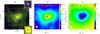 |
Fig. 2 Panel a: three-colour RGB image of CrA 151 obtained using the Herschel data at 500 (red), 250 (green), and 70 μm (blue). The contours show the distribution of the 350 μm SPIRE flux. The two square subpanels show zoom-ins of the core’s centre (bottom-right subpanel) and of the area around the YSO in the north-west of the core (top-right subpanel), with the 70 μm Herschel emission in magenta contours (levels: [25, 50, 150] MJy/sr; 1σ = 15 MJy/sr). The orange rectangle shows the region presented in the next two panels. Panels b and c: zoom-in of the map of the N(H2) distribution and of the dust temperature (or colour temperature, TC) from the HGBS survey. The beam size is shown in the bottom-left corners. In all panels, the coordinates of the core’s centre are shown with the ‘+’ symbol. |
3.3 Radiative transfer analysis
To model the observed spectra, we used the non-local-thermodynamic-equilibrium (non-LTE) radiative transfer code LOC (Juvela 2020). We used the hyperfine-splitted collisional rates taken from the EMAA catalogue4. The N2H+ rates were computed by Lique et al. (2015) and the N2D+ ones by Lin et al. (2020). To take into account additional line broadening due to turbulence, which is not considered in the physical model built so far, we manually added a constant contribution of σturb = 0.225 km s−1, chosen after a few tests in the range 0.075−0.3 km s−1. Since we do not have information on the gas kinetic temperature profile, we assumed Tgas = Tdust, where Tdust is derived from the modelling of the Herschel data shown in Fig. 3, which is a reasonable assumption because the dust and gas coupling is expected to be efficient at high densities (n ≳ 104 − 5 cm−3, Goldsmith 2001).
To estimate the N2H+ and N2D+ abundances, we performed a Markov chain Monte Carlo (MCMC) optimisation using the code EMCEE (Foreman-Mackey et al. 2013), following the approach of Jensen et al. (2024) and Ferrer Asensio et al. (2024). The free parameters are the constant abundance X(N2H+) of N2H+ and the constant deuteration fraction RD = X(N2D+)/X(N2H+). In addition, to take into account the uncertainties in the physical model computation, we allowed the entire density and temperature profiles to be multiplied by factors kn and kTK, respectively. We simultaneously fit the five available transitions, comparing the synthetic spectra produced by LOC to the observed one channel-by-channel and computing the χ2 for the minimisation. At each step, LOC was run with 50 iterations separately for the two isotopologues. The synthetic spectra were convolved to the angular resolutions listed in Table 1 and interpolated onto the spectral axes of the observations before computing the residuals. We first ran an initial simulation using 40 walkers for each free parameter and 500 steps. Then, we used the posterior distributions (in terms of medians and range) to select the initial set of parameters and their range for a second MCMC run (see Table 2). The first run was then discarded as burn-in. Figure C.1 shows the resulting corner plot, whilst Table 2 summarises the best parameter results. The code uses a logarithmic scale for the molecular abundance.
The synthetic spectra obtained with the median values of the free parameters are plotted in Fig. 1, and they generally agree with the observations, and the intensities of the N2H+ lines are reproduced well. The model fails to reproduce the double-peak asymmetry seen in the 3 – 2 line profile. This feature can be indicative of self-absorption combined with inward contraction motions. The fact that LOC cannot reproduce it could indicate that the physical model underestimates the contraction speed of the outskirts of the core or that we underestimated the N2H+ abundance in these regions, which is where most of the 3 – 2 flux likely arises. The observed linewidth of the N2H+ 5 − 4 line (the broadest in the sample; see Table 1) is underestimated by the model, a possible indication of increasing infall motions in the core’s centre, as discussed in Sect. 4. The profiles of the N2D+ lines are well reproduced. The peak intensities are slightly off, with the flux of the 3 − 2 line underpredicted, whilst the 4 − 3 and 6 – 5 synthetic spectra are brighter than the observations. However, for the highest J transition, the difference is comparable to the rms of the observed data.
The best-fit solution prefers a factor of about two denser physical structure than the model derived from the Herschel continuum data and a higher (by ∼40%) gas temperature. The temperature at the core centre is hence closer to 11 K, which is somewhat warmer than other typical pre-stellar sources. This could hint at the influence of the surrounding environment, as discussed further in Sect. 4. The main isotopologue abundance,  , is in line with estimates in similar sources (see Hardegree-Ullman et al. 2013 for CrA 151; Crapsi et al. 2005, Redaelli et al. 2018 in other dense cores). The deuteration level is high:
  , which is expected due to the high densities and relatively low temperatures that favour CO depletion and deuteration processes.
Parameters used in the MCMC analysis coupled with the radiative transfer algorithm LOC.
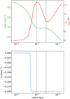 |
Fig. 3 Top panel: physical model of CrA 151 obtained from the Herschel data. The green curve (left y-axis) shows the total volume density n(H2), whilst the red curve (right y-axis) shows the dust temperature. The bumps in both profiles are due to a double Plummer-like structure. Bottom panel: velocity profile used for the MCMC modelling. In both panels, the vertical dashed and solid lines show the minimum and maximum resolution of the observations, from 13′′(N2H+ 5 − 4) to 37′′ (Herschel data). |
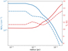 |
Fig. 4 Radial N(H2) and TC profiles of Cra 151 calculated from the Herschel maps shown in Fig. 2 (solid lines) and from the 1D (n, Tdust) model shown in Fig. 3 (dashed lines). |
3.4 Other lines identified
The large bandwidth of the APEX backend ensured that the collected observations have a broad frequency coverage, and they therefore cover the ranges 224.4−232.3, 240.6−248.5, 271.8−279.7, 287.3−295.9, 303.6−311.5, 462.2−466.2, and 474.6−478.6 GHz. We searched the whole frequency coverage to identify other lines. The complete list of detected transitions above S/N = 3 is given in Table D.1, and they are shown in Fig. 5. In total, we detected 35 transitions5 from 20 different species (including isotopologues).
All the nitrile transitions that fall in the covered frequency range were detected: CN 2 – 1, HNC 3 – 2, DCN 4 – 3, DNC 3 – 2, and 4 – 3. In addition, DCO+ 4 – 3 was also detected, with bright intensity (Tpeak ∼ 1.1 K).
Several transitions of methanol and the JKa Kc = 112−101(e0−o0) of doubly deuterated methanol were detected as well as two transitions for each deuterated isotopologue of formaldehyde. This confirms the high level of deuteration of the targeted core. We also detected triply deuterated ammonia ND3 and singly deuterated water HDO. Concerning S-bearing species, we detected CS (and the rarer C34S), SO, SO2, and HDS. Finally, we detected cyclic C3H2, protonated formaldehyde (H3CO+), and C17O.
Using the CLASS software, we performed Gaussian fits to the lines. In the case of CN and ND3, we fit only one hyperfine component; for C17O 2 − 1, which presents three unresolved components, we did not perform the fit. The best-fit parameters are also summarised in Table D.1.
The detected transitions present different line shapes, which can be divided into two groups. The deuterated species are usually well fit by the single Gaussian component assumption. The main exceptions are the HDS line (which fits better among the sulphurated species; see the discussion below) and possibly the HDCO 414−313 transition, where hints of a red shoulder can be seen. Species containing sulphur usually present a broad shoulder towards the higher velocities, up to ∼1 km s−1 above the core Vlsr. This shoulder is also identified in several other non-deuterated and non-sulphurated species, such as methanol, the main isotopologue of formaldehyde, CN and HCN. In some cases (e.g. HCN 3 − 2, SO 22 − 12), this feature resembles a second velocity component located at 6.0 – 6.2 km s−1.
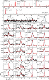 |
Fig. 5 Observed spectra of the species identified in the frequency coverage of the N2H+−N2D+ data (black histograms). The transitions are labelled in the top-left corner of each panel. The red histograms show the spectral fit performed with CLASS, which is a Gaussian fit for all transitions except for the ND3 and CN ones, for which we fit the hyperfine structure using the HFS routine. The vertical dotted line in each panel shows the source Vlsr = 5.65 km s−1, corresponding to the weighted average measured in the N2H+ and N2D+ lines. |
4 Discussion
Corona Australis 151 is a core well known for its high central density. Bresnahan et al. (2018) estimated an average density ⟨n⟩=107 cm−3 in the central 1000 au. This is confirmed by the detection of the high J transitions of N2H+ and N2D+ that we analysed in this work and by the fact that with our non-LTE models, we cannot reproduce both the low- and high-J transitions of N2H+ and N2D+ with volume densities lower than a few 107 cm−3, as shown in Appendix E. In particular, the N2H+ 5 − 4 and N2D+ 6 − 5 lines, observed with a linear resolution of ≈2000 au, have critical densities of 4 − 5 × 106 cm−3.
Our core model derived from Herschel maps at 160, 250, 350, and 500 μm is in agreement with this picture, with densities higher than 106 cm−3 within the central 5 × 10⁻³ pc = 1000 au, reaching a maximum of 3.2 × 107 cm−3 at ∼150 au. The average density within the central 1000 au is ∼6 × 106 cm−3. At the same time, the derived dust temperatures are low (Tdust < 12 K), which is consistent with pre-stellar gas in a quiescent environment. However, based on the available continuum data, we estimated a bolometric temperature for the core of Tbol = 18.7 K, which excludes significant internal heating from a protostellar source (Caselli et al., in prep.). The MCMC radiative transfer modelling of the lines is consistent with the high central density of the core (n ≈ 6 × 107 cm−3).
The comparison between the observational properties of dense cores and numerical simulations suggests that the dynamical evolution of an isolated prestellar core can be approximated by a sequence of hydrostatic cores in unstable equilibria, the so-called thermally supercritical Bonnor-Ebert spheres (BES; Foster & Chevalier 1993; Keto & Caselli 2010; Keto et al. 2015). The density profile of a supercritical BES approaches the power law n ∝ r−2 at large distances from the core centre, extending inwards to a point called the ‘flat radius’, which marks the radius where the sound crossing time equals the free-fall time. The flattened density region shrinks with time, whilst the central density increases, as also shown in ALMA observations of pre-stellar cores (Tokuda et al. 2020). In the marginally stable model, called the quasi-equilibrium (QE) BES model by Keto et al. (2015), the infall velocity reaches its maximum just outside the flat radius and goes to zero at the centre of the core and in the outer envelope. This feature clearly distinguishes the QE BES model from other collapse models, which often predict similar ∼r−2 density profiles but have very different infall velocity profiles. The QE BES model has been successfully used to interpret molecular line observations towards the prestellar core L1544 (Keto et al. 2015; Redaelli et al. 2019; Redaelli et al. 2021; Chacón-Tanarro et al. 2019; Rawlings et al. 2024). Keto et al. (2015) also discussed a non-equilibrium (NE) BES model that was constructed by increasing the density everywhere in an unstable BES, causing the sphere collapse on all scales. The infall velocity profile adopted here in the modelling of the observed spectra (Sect. 3.3) represents a crude approximation of the velocity distribution predicted by the NE BES model of Keto et al. (2015, see their Fig. 3). The fact that the N2H+ 5 – 4 and N2D+ 6 − 5 lines are detected in CrA 151 but not in L1544 (Caselli et al., in prep.) strongly suggests that CrA 151 has reached a higher central density than L1544. Whilst it is possible to reproduce the high-J transitions of both N2H+ and N2D+ with lower volume densities (3 – 6 × 106 cm−3) and higher N2H+ and N2D+ abundances, it is not possible to reproduce both lowand high-J transitions simultaneously without volume densities as high as 107 cm−3 (see also Appendix E). The density profile of CrA 151 shown in Fig. 3 agrees with the r−2 power law, except for the depression around r = 0.01 pc, which is accompanied by a bump in the dust temperature profile. These features are invoked by corresponding bumps in the intensity profiles at 160 and 250 μm. The irregularities may be understood as deviations from the idealised models described above, where particles are always accelerated towards the centre, and no shocks occur when the infall speed exceeds the sound speed (Foster & Chevalier 1993).
Thus, CrA 151 probably represents a more advanced stage of prestellar core evolution than L1544. We have three pieces of evidence in support of this hypothesis. Firstly, there is the detection of compact 70 μm emission at the centre of the core, with a flux density of 0.15 ± 0.03 Jy (Bresnahan et al. 2018). Secondly, the increasing linewidth of the N2H+ and N2D+ lines with increasing frequency points towards faster motions in the central denser regions of the core. Thirdly, several lines present high-velocity wings (up to ∼1 km s−1 above the source Vlsr; see Sect. 3.4). With the present data from a single pointing, we cannot rule out the possibility that the high-velocity wings are caused by external influence, for example, by an outflow from the nearby protostar lying approximately 0.4 pc to the northwest of the core (Esplin & Luhman 2022, see also Panel a of Fig. 2). To our knowledge, no search for protostellar outflows has been conducted in this region, and we cannot exclude that this source is launching an outflow that is affecting the properties of CrA 151. Another possibility, however, is the presence of supersonic infall motions. In regard to these possibilities, we tested a velocity profile that includes them, and the results are compatible with the observed lines of N2H+ and N2D+. However, observations at a higher resolution, as well as a dedicated model, are needed to confirm the presence of a supersonic infall. Although our MCMC analysis does not suggest a need for higher central temperatures to reproduce the observed lines of N2H+ and N2D+ and the very large deuterium fractionation measured also supports the pre-stellar core option, it is possible that all three pieces of evidence listed above are manifestations of a very young protostar.
A greybody fit to the flux densities from 70 to 850 μm (combining the data from the HGBS archive with the 850 μm aperture flux from SCUBA, 1.6 ± 0.1 Jy) gives a bolometric temperature of 18.7 K and a bolometric luminosity of 0.1 L⊙ for the core. The latter value is an upper limit for the luminosity of the possible central source, which should therefore be classified as a VeLLO. The 70 μm map was excluded in the derivation of the core model because the compact low-intensity source is smoothed out when convolved with the Herschel 500 μm beam. We tested how the model should be modified in order to reproduce the observed 70 μm map. Adopting the density structure of our model but assuming a uniform temperature throughout the core, the best fit to the observed map was obtained with T = 14 K. This suggests that the temperature is indeed elevated in the very centre, although lower resolution data give 8 K (3D model) or 10 K (TC from Herschel). In view of severe obscuration from the interstellar radiation field, a central temperature of 14 K would imply internal heating, either by shocks in the accreting material or outflows. In case the core contains an FHSC, the central density should exceed 10−12 g cm−3, corresponding to n(H2) ∼ 1011 cm3 (e.g. Young et al. 2019). The spectral wings observed for the sulphurated molecules may trace a low-velocity outflow, which is expected from an FHSC (Machida et al. 2008; Fujishiro et al. 2020).
The high central densities cause CO depletion, as investigated by Hardegree-Ullman et al. (2013). In turn, the depletion of CO molecules onto dust grains, combined with the low temperature, increases the efficiency of deuteration processes, as the production of H2D+ is favoured. The high level of deuteration of CrA 151 is confirmed by analysis of the diazenylium lines. The radiative transfer analysis implies a deuteration level of 50%. For comparison, the N2D+/N2H+ ratio in L1544 is 26% (Redaelli et al. 2019); Friesen et al. (2013) found RD ≲ 0.20 in a sample of starless cores in Perseus; in the L1688 region in Ophiuchus, Punanova et al. (2018) reported a deuteration fraction in the range of 2 − 40%. In a twin work dedicated to another of the densest cores in the sample (Oph 464, or IRAS16293E), Spezzano et al. (2025) found values as high as 44%. The high deuteration level of CrA 151 is corroborated by the number of deuterated species detected (see Sect. 3.4), including doubly (CHD2OH, D2CO) and triply (ND3) deuterated isotopologues. We also report the first detection of deuterated water in a pre-stellar environment.
The modelling we performed bears several limitations. The first is the usage of a spherically symmetric model. The dust continuum maps shown in Fig. 2 clearly deviate from spherical symmetry around the core’s centre. Nevertheless, this approximation seems reasonable within the central ∼2′, which is comparable to the simulated core radius (0.14 pc or 190′′). Furthermore, the development of a fully three-dimensional core structure goes beyond the scope of the present paper, which intends to investigate the physical conditions at the core’s centre. The MCMC analysis could also be expanded by introducing more free parameters, such as the velocity profile or the turbulence contribution. However, increasing the number of free parameters whilst maintaining the same number of observational constraints (the five N2H+ and N2D+ lines) does not guarantee better convergence of the method, as also discussed by Jensen et al. (2024). Therefore, we preferred to focus on the parameters that are more relevant to our analysis: density, temperature, and the abundance of the two species.
It is worth commenting on the choice of constant abundance for N2H+ and N2D+. As discussed in Sect. 3.3, these profiles reproduce the line profiles and the intensity ratio of the distinct J transitions reasonably well, even though there is a tendency to overestimate the fluxes of the high-frequency transitions of N2D+ (by 200 mK for N2D+ 4 − 3, and by 50 mK for N2D+ 6 – 5; the rms levels of the two lines are 9 and 29 mK, respectively). Since the high-J transitions have a higher critical density and thus are emitted closer to the core’s centre, the modelling could benefit from some level of depletion in the central parts of the core. However, the situation is different from the case of L1544, where if the N2D+ abundance profile is kept constant in the central ≈4000 au, the higher −J transitions are overestimated by a factor of two or more compared to the low-J transition (Redaelli et al. 2019)6. Instead, CrA 151 resembles the situation of IRAS16293E analysed by Spezzano et al. (2025), where the authors concluded that models with either no depletion or with a small central depletion zone of ≲ 1000 au can reproduce the observations.
These findings are in disagreement with chemical models, which in general predict some level of N2 (and thus N2H+ and N2D+) depletion at high densities (see Sipilä et al. 2019) and low temperatures. The limited angular resolution of our observations might play a role. In L1544, the depletion of NH3 is detected only with ALMA high-resolution (400 au) observations (Caselli et al. 2022). Furthermore, the core temperatures derived with the MCMC analysis in CrA 151(12 − 16 K) are higher than those detected in other quiescent cores, where Tgas ≲ 10 K (Crapsi et al. 2007; Lin et al. 2023).
5 Summary and conclusions
We have reported on the detection of the N2H+ 3 − 2 and 5 – 4 and the N2D+ 3 − 2, 4 − 3, and 6 – 5 lines towards the dense core CrA 151 using the APEX single-dish telescope. This core was selected for further investigation and modelling from the sample of dense starless sources collected from the Herschel HGBS catalogue (Caselli et al., in prep.). Analysing the Herschel continuum maps, we built a spherical model of the source characterised by high central densities (n ≳ 107 cm−3) and overall low dust temperatures (8 − 12 K).
Starting from a 1D model, we modelled the spectra using non-LTE radiative transfer coupled with MCMC analysis using the abundance of N2H+ and its deuterium fraction as free parameters. We also let the density and temperature profiles vary by constant factors. This modelling predicts that even higher densities (a factor of about two) and warmer temperatures (factor of ∼1.4) than those derived from the Herschel fluxes are needed to reproduce the observations. Constant abundance profiles of X(N2H+) ∼ 10−10 and X(N2D+) ∼ 5 × 10⁻¹¹ are in reasonable agreement with the APEX spectra even though we cannot exclude some level of depletion limited to the central ≈1000 au. The derived deuterium fraction is 50%. This deuteration, enhanced by the high densities and relatively low gas temperature, is among the highest levels seen in similar sources.
In the large frequency coverage of the APEX data, we detected 20 other species, including several deuterated isotopologues. The detection of CHD2OH, D2CO, and ND3 highlights the generally high levels of deuteration of the source. These transitions are well fit by single Gaussian components with narrow linewidths (FWHM ≲ 0.5 km s−1). This evidence supports the scenario of a dense and cold quiescent core. However, the other detected species, in particular sulphur-bearing ones, often show line profiles with extended wings at high velocities (Vlsr > 6 km s−1). There are three possible ways to interpret these profiles: (i) they show the possible influence of the surrounding environment, where at least one protostar has been identified at a projected distance of 0.4 pc; (ii) they indicate the presence of a very young embedded protostar or an FHSC; (iii) or they result from the presence of supersonic infall motions in the central parts of the core. The latter scenario is supported by the fact that for diazenylium, we observed an increase of intrinsic linewidth as the critical density and angular resolution of the transitions increase, the high level of deuterium fractionation measured for N2H+, and the physical modelling of the source, which points towards an evolved dynamical pre-stellar core.
The spectral features mentioned above and the detection of faint 70 μm emission suggest the presence of an internal heating source in CrA 151. With an upper limit of 0.1 L⊙, the hypothetical central source would fall in the category of VeLLOs and is thereby also a candidate FHSC. CrA 151 may represent the very short and elusive phase when a prestellar core is transforming itself into a protostellar core. As an isolated nearby object, CrA 151 is an ideal target for future high-resolution (tens to hundreds au) continuum and spectral line observations investigating the innermost structure of a dense core; the kinematics of the infalling gas; and, if the core already contains a protostar or an FHSC, the earliest stages of a molecular outflow.
Acknowledgements
The data was collected under the Atacama Pathfinder EXperiment (APEX) Project, led by the Max Planck Institute for Radio Astronomy at the ESO La Silla Paranal Observatory. This research has made use of data from the Herschel Gould Belt survey (HGBS) project (http://gouldbelt-herschel.cea.fr). The HGBS is a Herschel Key Programme jointly carried out by SPIRE Specialist Astronomy Group 3 (SAG 3), scientists of several institutes in the PACS Consortium (CEA Saclay, INAF-IFSI Rome and INAF-Arcetri, KU Leuven, MPIA Heidelberg), and scientists of the Herschel Science Center (HSC). This research has made use of spectroscopic and collisional data from the EMAA database (https://emaa.osug.fr and https://dx.doi.org/10.17178/EMAA). EMAA is supported by the Observatoire des Sciences de l’Univers de Grenoble (OSUG).
Appendix A CLASS HFS fit
In Fig. A.1 we show the best-fit solutions found with the CLASS HFS fitting routine, as described in Sect. 3.1.
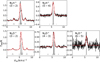 |
Fig. A.1 N2H+ and N2D+ spectra (black histograms) and the best-fit solution found by CLASS (red histograms), assuming the same excitation temperature for all the hyperfine components. The vertical black lines show the position of the hyperfine components; their length is proportional to the relative intensities. |
Appendix B Herschel maps
Figure B.1 shows the Herschel data of CrA 151 from the SPIRE and PACS instruments in the top row. The corresponding bottom panels show the intensity profiles, circularly averaged around the core’s centre.
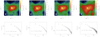 |
Fig. B.1 Top row: Herschel SPIRE and PACS maps. Bottom row: Corresponding circularly averaged intensity profiles. One can note the broader emission at large radii in the 160 and 250 μm maps that require two Plummer profiles for an optimal fit. The 160, 250, and 350 μm maps have been smoothed to the resolution of the 500 μm one. |
Appendix C MCMC results
Figure C.1 shows the corner plots of the final MCMC run performed using LOC, fitting simultaneously the five diazenylium transitions.
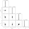 |
Fig. C.1 Corner plots of the MCMC+LOC modelling of the five N2H+ and N2D+ lines towards the target. The title of each corner reports the 50th percentile (median), together with the 16th and 84th percentiles as negative and positive uncertainties, respectively. |
Appendix D Parameters of identified lines
Table D.1 shows the complete list of lines detected in the frequency range covered by the APEX data, together with the best-fit parameters obtained from spectral fit.
Lines robustly detected (S/N > 3) in the spectral ranges covered by the observations.
Appendix E LOC tests
Figure E.1 shows the output of LOC for N2H+ using the input profiles of the best model shown in the paper (see Fig. 1). Here, we have reduced the volume density by a factor of 10 (upper panel) and 5 (lower panel), and increased the N2H+ abundance accordingly to find a good match with the observations. The results show that if the volume density is not high enough, the column densities necessary to reproduce the high- J transition are too high for the low- J transitions.
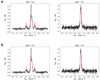 |
Fig. E.1 LOC tests with lower volume density. Panel (a): we scaled down the volume density profile used for the results shown in Fig. 1 by a factor of 10 and scaled up the abundance profile of N2H+ by a factor of 45 in the effort of reproducing the observed lines. Panel (b): we reduced the volume density profile used in Fig. 1 by a factor of 5 and scaled up the abundance profile of N2H+ by a factor of 15. In both cases, we show that it is not possible to reproduce both transitions with a lower volume density by only increasing the abundance of N2H+. |
References
- André, P., Men’shchikov, A., Bontemps, S., et al. 2010, A&A, 518, L102 [NASA ADS] [CrossRef] [EDP Sciences] [Google Scholar]
- Bechtel, H. A., Steeves, A. H., & Field, R. W. 2006, ApJ, 649, L53 [CrossRef] [Google Scholar]
- Bocquet, R., Demaison, J., Cosléou, J., et al. 1999, J. Mol. Spectr., 195, 345 [Google Scholar]
- Bogey, M., Demuynck, C., & Destombes, J. L. 1986, Chem. Phys. Lett., 125, 383 [NASA ADS] [CrossRef] [Google Scholar]
- Bresnahan, D., Ward-Thompson, D., Kirk, J. M., et al. 2018, A&A, 615, A125 [NASA ADS] [CrossRef] [EDP Sciences] [Google Scholar]
- Brünken, S., Müller, H. S. P., Thorwirth, S., et al. 2006, J. Mol. Struc., 780, 3 [Google Scholar]
- Caselli, P., & Dore, L. 2005, A&A, 433, 1145 [NASA ADS] [CrossRef] [EDP Sciences] [Google Scholar]
- Caselli, P., Pineda, J. E., Zhao, B., et al. 2019, ApJ, 874, 89 [NASA ADS] [CrossRef] [Google Scholar]
- Caselli, P., Pineda, J. E., Sipilä, O., et al. 2022, [arXiv:2202.13374] [Google Scholar]
- Cazzoli, G., Dore, L., Puzzarini, C., et al. 2002, Phys. Chem. Chem. Phys., 4, 3575 [Google Scholar]
- Ceccarelli, C., Caselli, P., Bockelée-Morvan, D., et al. 2014, in Protostars and Planets VI, eds. H. Beuther, R. S. Klessen, C. P. Dullemond, & T. Henning (Tucson: University of Arizona Press), 859 [Google Scholar]
- Chacón-Tanarro, A., Caselli, P., Bizzocchi, L., et al. 2019, A&A, 622, A141 [Google Scholar]
- Chini, R., Kämpgen, K., Reipurth, B., et al. 2003, A&A, 409, 235 [NASA ADS] [CrossRef] [EDP Sciences] [Google Scholar]
- Clark, W. W., & De Lucia, F. C. 1976, J. Mol. Spectr., 60, 332 [Google Scholar]
- Commerçon, B., Launhardt, R., Dullemond, C., et al. 2012, A&A, 545, A98 [NASA ADS] [CrossRef] [EDP Sciences] [Google Scholar]
- Crapsi, A., Caselli, P., Walmsley, C. M., et al. 2005, ApJ, 619, 379 [Google Scholar]
- Crapsi, A., Caselli, P., Walmsley, M. C., & Tafalla, M. 2007, A&A, 470, 221 [NASA ADS] [CrossRef] [EDP Sciences] [Google Scholar]
- Dalgarno, A., & Lepp, S. 1984, ApJ, 287, L47 [NASA ADS] [CrossRef] [Google Scholar]
- di Francesco, J., Evans, N. J., Caselli, P., et al. 2007, Protostars and Planets V (Tucson: University of Arizona Press), 17 [Google Scholar]
- Esplin, T. L., & Luhman, K. L. 2022, AJ, 163, 64 [NASA ADS] [CrossRef] [Google Scholar]
- Evans, N. J. 1999, ARA&A, 37, 311 [NASA ADS] [CrossRef] [Google Scholar]
- Ferrer Asensio, J., Jensen, S. S., Spezzano, S., et al., 2024, ApJ, submitted [Google Scholar]
- Foreman-Mackey, D., Hogg, D. W., Lang, D., & Goodman, J. 2013, PASP, 125, 306 [Google Scholar]
- Foster, P. N., & Chevalier, R. A. 1993, ApJ, 416, 303 [NASA ADS] [CrossRef] [Google Scholar]
- Friesen, R. K., Kirk, H. M., & Shirley, Y. L. 2013, ApJ, 765, 59 [NASA ADS] [CrossRef] [Google Scholar]
- Fujishiro, K., Tokuda, K., Tachihara, K., et al. 2020, ApJ, 899, L10 [Google Scholar]
- Galli, D., & Shu, F. H. 1993, ApJ, 417, 243 [NASA ADS] [CrossRef] [Google Scholar]
- Galli, P. A. B., Bouy, H., Olivares, J., et al. 2020, A&A, 634, A98 [NASA ADS] [CrossRef] [EDP Sciences] [Google Scholar]
- Goldsmith, P. F. 2001, ApJ, 557, 736 [Google Scholar]
- Güsten, R., Nyman, L. Å., Schilke, P., et al. 2006, A&A, 454, L13 [NASA ADS] [CrossRef] [EDP Sciences] [Google Scholar]
- Hardegree-Ullman, E., Harju, J., Juvela, M., et al. 2013, ApJ, 763, 45 [Google Scholar]
- Helminger, P., & Gordy, W. 1969, Phys. Rev., 188, 100 [NASA ADS] [CrossRef] [Google Scholar]
- Helminger, P., Cook, R. L., & De Lucia, F. C. 1971, J. Mol. Spectr., 40, 125 [Google Scholar]
- Hildebrand, R. H. 1983, QJRAS, 24, 267 [NASA ADS] [Google Scholar]
- Hily-Blant, P., Walmsley, M., Pineau Des Forêts, G., & Flower, D. 2010, A&A, 513, A41 [NASA ADS] [CrossRef] [EDP Sciences] [Google Scholar]
- Jensen, S. S., Spezzano, S., Caselli, P., et al. 2024, A&A, 685, A149 [NASA ADS] [CrossRef] [EDP Sciences] [Google Scholar]
- Juvela, M. 2020, A&A, 644, A151 [NASA ADS] [CrossRef] [EDP Sciences] [Google Scholar]
- Keto, E., & Caselli, P. 2010, MNRAS, 402, 1625 [Google Scholar]
- Keto, E., Caselli, P., & Rawlings, J. 2015, MNRAS, 446, 3731 [NASA ADS] [CrossRef] [Google Scholar]
- Klapper, G., Surin, L., Lewen, F., et al. 2003, ApJ, 582, 262 [NASA ADS] [CrossRef] [Google Scholar]
- Dixon, T. A., & Woods, R. C. 1977, J. Chem. Phys., 67, 3956 [CrossRef] [Google Scholar]
- Klein, T., Ciechanowicz, M., Leinz, C., et al. 2014, IEEE Trans. Terahertz Sci. Technol., 4, 588 [CrossRef] [Google Scholar]
- Larson, R. B. 1969, MNRAS, 145, 271 [Google Scholar]
- Lin, S.-J., Pagani, L., Lai, S.-P., Lefèvre, C., & Lique, F. 2020, A&A, 635, A188 [EDP Sciences] [Google Scholar]
- Lin, Y., Spezzano, S., Pineda, J. E., et al. 2023, A&A, 680, A43 [NASA ADS] [CrossRef] [EDP Sciences] [Google Scholar]
- Lique, F., Daniel, F., Pagani, L., & Feautrier, N. 2015, MNRAS, 446, 1245 [NASA ADS] [CrossRef] [Google Scholar]
- Machida, M. N., Inutsuka, S.-. ichiro., & Matsumoto, T. 2008, ApJ, 676, 1088 [CrossRef] [Google Scholar]
- Melosso, M., Bizzocchi, L., Dore, L., et al. 2021, J. Mol. Spectr., 377, 111431 [Google Scholar]
- Messer, J. K., De Lucia, F. C., & Helminger, P. 1984, J. Mol. Spectr., 105, 139 [Google Scholar]
- Müller, H. S. P., & Lewen, F. 2017, J. Mol. Spectr., 331, 28 [CrossRef] [Google Scholar]
- Müller, H. S. P., Schlöder, F., Stutzki, J., et al. 2005, J. Mol. Struc., 742, 215 [CrossRef] [Google Scholar]
- Pickett, H. M., Poynter, R. L., Cohen, E. A., et al. 1998, J. Quant. Spec. Radiat. Transf., 60, 883 [Google Scholar]
- Punanova, A., Caselli, P., Pineda, J. E., et al. 2018, A&A, 617, A27 [NASA ADS] [CrossRef] [EDP Sciences] [Google Scholar]
- Rawlings, J. M. C., Keto, E., & Caselli, P. 2024, MNRAS, 530, 3986 [Google Scholar]
- Redaelli, E., Bizzocchi, L., Caselli, P., et al. 2018, A&A, 617, A7 [NASA ADS] [CrossRef] [EDP Sciences] [Google Scholar]
- Redaelli, E., Bizzocchi, L., Caselli, P., et al. 2019, A&A, 629, A15 [NASA ADS] [CrossRef] [EDP Sciences] [Google Scholar]
- Redaelli, E., Sipilä, O., Padovani, M., et al. 2021, A&A, 656, A109 [NASA ADS] [CrossRef] [EDP Sciences] [Google Scholar]
- Roy, A., André, P., Palmeirim, P., et al. 2014, A&A, 562, A138 [NASA ADS] [CrossRef] [EDP Sciences] [Google Scholar]
- Sandqvist, A., & Lindroos, K. P. 1976, A&A, 53, 179 [NASA ADS] [Google Scholar]
- Saykally, R. J., Szanto, P. G., Anderson, T. G., et al. 1976, ApJ, 204, L143 [NASA ADS] [CrossRef] [Google Scholar]
- Shirley, Y. L. 2015, PASP, 127, 299 [Google Scholar]
- Sicilia-Aguilar, A., Henning, T., Linz, H., et al. 2013, A&A, 551, A34 [NASA ADS] [CrossRef] [EDP Sciences] [Google Scholar]
- Sipilä, O., Caselli, P., Redaelli, E., Juvela, M., & Bizzocchi, L. 2019, MNRAS, 487, 1269 [Google Scholar]
- Spezzano, S., Redaelli, E., Caselli, P., et al. 2025, A&A, 694, A27 [NASA ADS] [CrossRef] [EDP Sciences] [Google Scholar]
- Tokuda, K., Fujishiro, K., Tachihara, K., et al. 2020, ApJ, 899, 10 [NASA ADS] [CrossRef] [Google Scholar]
- Tomida, K., Machida, M. N., Saigo, K., et al. 2010, ApJ, 725, L239 [NASA ADS] [CrossRef] [Google Scholar]
- Xu, L.-H., Fisher, J., Lees, R. M., et al. 2008, J. Mol. Spectr., 251, 305 [NASA ADS] [CrossRef] [Google Scholar]
- Young, A. K., Bate, M. R., Harries, T. J., et al. 2019, MNRAS, 487, 2853 [NASA ADS] [CrossRef] [Google Scholar]
- Zakharenko, O., Motiyenko, R. A., Margulès, L., et al. 2015, J. Mol. Spectr., 317, 41 [Google Scholar]
All data available at http://gouldbelt-herschel.cea.fr/archives
Available at http://www.iram.fr/IRAMFR/GILDAS/
Available at https://emaa.osug.fr/species-list
We consider here a single value for the CN J = 2 − 1 line, even though the whole fine structure pattern was observed, and for the hyperfine structure of ND3 101 − 000 and C17 O 2 − 1.
In that paper, the authors analysed N2D+ 1 − 0, 2 − 1, and 3 – 2. The 4 – 3 and 6 − 5 transitions are not detected in L1544 (Caselli et al., in prep.).
All Tables
Parameters used in the MCMC analysis coupled with the radiative transfer algorithm LOC.
Lines robustly detected (S/N > 3) in the spectral ranges covered by the observations.
All Figures
|
Fig. 1 Observations of the N2H+ and N2D+ transitions towards CrA 151 (black histograms) and synthetic spectra obtained with the MCMC approach applied to the non-LTE radiative transfer analysis (red histograms; see Sect. 3.3). |
| In the text | |
|
Fig. 2 Panel a: three-colour RGB image of CrA 151 obtained using the Herschel data at 500 (red), 250 (green), and 70 μm (blue). The contours show the distribution of the 350 μm SPIRE flux. The two square subpanels show zoom-ins of the core’s centre (bottom-right subpanel) and of the area around the YSO in the north-west of the core (top-right subpanel), with the 70 μm Herschel emission in magenta contours (levels: [25, 50, 150] MJy/sr; 1σ = 15 MJy/sr). The orange rectangle shows the region presented in the next two panels. Panels b and c: zoom-in of the map of the N(H2) distribution and of the dust temperature (or colour temperature, TC) from the HGBS survey. The beam size is shown in the bottom-left corners. In all panels, the coordinates of the core’s centre are shown with the ‘+’ symbol. |
| In the text | |
|
Fig. 3 Top panel: physical model of CrA 151 obtained from the Herschel data. The green curve (left y-axis) shows the total volume density n(H2), whilst the red curve (right y-axis) shows the dust temperature. The bumps in both profiles are due to a double Plummer-like structure. Bottom panel: velocity profile used for the MCMC modelling. In both panels, the vertical dashed and solid lines show the minimum and maximum resolution of the observations, from 13′′(N2H+ 5 − 4) to 37′′ (Herschel data). |
| In the text | |
|
Fig. 4 Radial N(H2) and TC profiles of Cra 151 calculated from the Herschel maps shown in Fig. 2 (solid lines) and from the 1D (n, Tdust) model shown in Fig. 3 (dashed lines). |
| In the text | |
|
Fig. 5 Observed spectra of the species identified in the frequency coverage of the N2H+−N2D+ data (black histograms). The transitions are labelled in the top-left corner of each panel. The red histograms show the spectral fit performed with CLASS, which is a Gaussian fit for all transitions except for the ND3 and CN ones, for which we fit the hyperfine structure using the HFS routine. The vertical dotted line in each panel shows the source Vlsr = 5.65 km s−1, corresponding to the weighted average measured in the N2H+ and N2D+ lines. |
| In the text | |
|
Fig. A.1 N2H+ and N2D+ spectra (black histograms) and the best-fit solution found by CLASS (red histograms), assuming the same excitation temperature for all the hyperfine components. The vertical black lines show the position of the hyperfine components; their length is proportional to the relative intensities. |
| In the text | |
|
Fig. B.1 Top row: Herschel SPIRE and PACS maps. Bottom row: Corresponding circularly averaged intensity profiles. One can note the broader emission at large radii in the 160 and 250 μm maps that require two Plummer profiles for an optimal fit. The 160, 250, and 350 μm maps have been smoothed to the resolution of the 500 μm one. |
| In the text | |
|
Fig. C.1 Corner plots of the MCMC+LOC modelling of the five N2H+ and N2D+ lines towards the target. The title of each corner reports the 50th percentile (median), together with the 16th and 84th percentiles as negative and positive uncertainties, respectively. |
| In the text | |
|
Fig. E.1 LOC tests with lower volume density. Panel (a): we scaled down the volume density profile used for the results shown in Fig. 1 by a factor of 10 and scaled up the abundance profile of N2H+ by a factor of 45 in the effort of reproducing the observed lines. Panel (b): we reduced the volume density profile used in Fig. 1 by a factor of 5 and scaled up the abundance profile of N2H+ by a factor of 15. In both cases, we show that it is not possible to reproduce both transitions with a lower volume density by only increasing the abundance of N2H+. |
| In the text | |
Current usage metrics show cumulative count of Article Views (full-text article views including HTML views, PDF and ePub downloads, according to the available data) and Abstracts Views on Vision4Press platform.
Data correspond to usage on the plateform after 2015. The current usage metrics is available 48-96 hours after online publication and is updated daily on week days.
Initial download of the metrics may take a while.