| Issue |
A&A
Volume 696, April 2025
|
|
|---|---|---|
| Article Number | A153 | |
| Number of page(s) | 20 | |
| Section | Astronomical instrumentation | |
| DOI | https://doi.org/10.1051/0004-6361/202451951 | |
| Published online | 17 April 2025 | |
ALeRCE light curve classifier: Tidal disruption event expansion pack
1
Instituto de Astrofísica, Facultad de Física, Pontificia Universidad Católica de Chile, Campus San Joaquín,
Av. Vicuña Mackenna 4860,
Macul Santiago
7820436,
Chile
2
Millennium Institute of Astrophysics (MAS),
Nuncio Monseñor Sótero Sanz 100,
Providencia, Santiago,
Chile
3
Departamento de Astronomía, Universidad de Chile,
Casilla 36D,
Santiago,
Chile
4
European Southern Observatory,
Karl-Schwarzschild-Strasse 2,
85748
Garching bei München,
Germany
5
Millennium Nucleus on Transversal Research and Technology to Explore Supermassive Black Holes (TITANS),
4030000
Concepción,
Chile
6
Instituto de Física y Astronomía, Facultad de Ciencias, Universidad de Valparaíso,
Gran Bretana 1111,
Playa Ancha, Valparaíso,
Chile
7
Centro de Astroingeniería, Facultad de Física, Pontificia Universidad Católica de Chile, Campus San Joaquín,
Av. Vicuña Mackenna 4860,
Macul Santiago
7820436,
Chile
8
Space Science Institute,
4750 Walnut Street, Suite 205, Boulder,
Colorado
80301,
USA
9
Data and Artificial Intelligence Initiative (IDIA), Faculty of Physical and Mathematical Sciences, Universidad de Chile,
Chile
10
Center for Mathematical Modeling, Universidad de Chile,
Beauchef 851,
Santiago
8370456,
Chile
11
Instituto de Estudios Astrofísicos, Facultad de Ingeniería y Ciencias, Universidad Diego Portales,
Av. Ejército Libertador 441,
Santiago,
Chile
12
Kavli Institute for Astronomy and Astrophysics, Peking University,
Beijing
100871,
China
13
Data Observatory Foundation,
Santiago,
Chile
14
Institute of Astronomy, KU Leuven,
Celestijnenlaan 200D,
3001
Leuven,
Belgium
15
Department of Computer Science, Universidad de Concepción,
Concepción,
Chile
16
Data Science Unit, Universidad de Concepción,
Edmundo Larenas 310,
Concepción,
Chile
★ Corresponding author; This email address is being protected from spambots. You need JavaScript enabled to view it.
Received:
22
August
2024
Accepted:
21
February
2025
Abstract
Context. ALeRCE (Automatic Learning for the Rapid Classification of Events) is currently processing the Zwicky Transient Facility (ZTF) alert stream, in preparation for the Vera C. Rubin Observatory, and classifying objects using a broad taxonomy. The ALeRCE light curve classifier is a balanced random forest (BRF) algorithm with a two-level scheme that uses variability features computed from the ZTF alert stream, and colors obtained from AllWISE and ZTF photometry.
Aims. This work develops an updated version of the ALeRCE broker light curve classifier that includes tidal disruption events (TDEs) as a new subclass. For this purpose we incorporated 24 new features, notably including the distance to the nearest source detected in ZTF science images and a parametric model of the power-law decay for transients. We also expanded the labeled set to include 219 792 spectroscopically classified sources, including 60 TDEs.
Methods. To effectively integrate TDEs into the ALeRCE’s taxonomy, we identified specific characteristics that set them apart from other transient classes, such as their central position in a galaxy, the typical decay pattern displayed when fully disrupted, and the lack of color variability after disruption. Based on these attributes, we developed features to distinguish TDEs from other transient events.
Results. The modified classifier can distinguish between a broad range of classes with a better performance compared to the previous version and it can integate the TDE class achieving 91% recall, also identifying a large number of potential TDE candidates in ZTF alert stream unlabeled data.
Key words: methods: data analysis / methods: numerical
© The Authors 2025
 Open Access article, published by EDP Sciences, under the terms of the Creative Commons Attribution License (https://creativecommons.org/licenses/by/4.0), which permits unrestricted use, distribution, and reproduction in any medium, provided the original work is properly cited.
This article is published in open access under the Subscribe to Open model. This email address is being protected from spambots. You need JavaScript enabled to view it. to support open access publication.
1 Introduction
Tidal disruption events (TDEs) are caused by the disruption of stars (or compact objects) around massive black holes at the center of most galaxies, and they were first theorized in the late 1970s (Hills 1975). The fate of a star near a black hole depends on the relative sizes of both the tidal disruption radius and event horizon. If a star is disrupted outside the event horizon (for solar-type stars, this occurs when 105 M⊙ ≤ MBH ≤ 108 M⊙; Rees 1988), a luminous burst of energy is expected to occur related to the fraction of tidal debris that falls back onto the black hole. The debris stream circularizes and forms an accretion disk, generating emission across the electromagnetic spectrum (Rees 1988; Phinney 1989; Evans & Kochanek 1989; Ulmer 1999). TDEs are characterized by certain features such as hydrogen and helium emission lines in their optical spectrum, non-varying blue continuum in optical filters, and a flux decay rate that theoretically scales as ∝ t−5/3 for a full disruption (as stated in van Velzen et al. 2021) which is deeply related to the mass infall rate (Evans & Kochanek 1989). Over the past decade, ~100 TDEs have been discovered. These events have a central position in a galaxy and have a timescale for the fallback and circularization of the stellar debris streams as short as a few months (van Velzen et al. 2021; Hammerstein et al. 2022; Yao et al. 2023). TDEs are relatively rare at the limits of past and current time domain surveys, with a rate 1.3 ± 0.2 × 10⁻⁷ Mpc−3 year−1 (Masterson et al. 2024). As such, understanding their nature, origin, and evolution has been difficult. The discovery of more of these events, while challenging, can greatly advance the field.
In the current era of time domain (TD) astronomy, the Zwicky Transient Facility (ZTF) at Palomar Observatory (Dekany et al. 2016; Bellm et al. 2019) has been identifying high-quality transients each year, but a low number of them can be classified spectroscopically due to limited resources; this issue will become more severe when the Legacy Survey of Space and Time (LSST) on the Vera C. Rubin Observatory commences and increases the number of transients detected by two orders of magnitude (Ivezić et al. 2019). Other examples of TD surveys are ASAS-SN (Jayasinghe et al. 2019b) or Gaia (Mowlavi et al. 2018); we refer readers to Figure 1 of Förster et al. (2021) for an idea of the number of ongoing and planned TD surveys or Catelan (2023) for a more recent review on ground-based time-domain surveys. In this context, astronomical brokers have been processing the alert streams of these astronomical surveys, and in particular ALeRCE (Automatic Learning for the Rapid Classification of Events; Förster et al. 2021) has been processing the ZTF public alert stream since 2019 and has developed machine learning (ML) tools for the classification of these alerts in real time. The goal of this current work is to update the light curve classifier from Sánchez-Sáez et al. (2021) (hereafter lc_classifier and SS21, respectively), which is comprised of a two-level balanced random forest (BRF), capable of differentiating sources between 15 subclasses that define the ALeRCE taxonomy. The goal of this kind of ML algorithm is to circumvent the bottleneck created by limited spectroscopic resources, and ultimately provide highly effective (i.e., both high purity and completeness) candidate selection using only light curve and other ancillary information. Although the previous version of this light curve classifier discussed in SS21 included numerous subclasses, it did not include the TDE class due to the very small number of confirmed TDEs available at the time of training and testing. To the best of our knowledge, three ML-based classifiers include the TDE class: Finding Luminous and Exotic Extragalactic Transients (FLEET; Gomez et al. 2023), tdescore (Stein et al. 2024), and NEural Engine for Discovering Luminous Events (NEEDLE; Sheng et al. 2024).
Since the publication of SS21, the number of sources in the labeled set of ALeRCE (Förster et al. 2021) has increased significantly. Not only have the observed examples in the classes within the lc_classifier increased in number, but a substantial number of TDEs have also been confirmed, sufficient for both training and testing purposes. From the original classifier model, we have an extensive range of features (152) and we aim to integrate TDEs into the taxonomy. To facilitate this integration and enhance performance, we developed a new set of features specifically tuned to distinguish TDEs from other transient classes. In this paper we present an update to the lc_classifier, the second version of our photometric-based ML classifier, that can now classify 16 subclasses using 176 features. The improvements of the update are mainly reflected by the recall and precision of the transient branch confusion matrix.
This paper is organized as follows. In Sect. 2, we describe the methodologies for this work, including how the reference data were obtained (Sect. 2.1), the new classification taxonomy Sect. 2.2), the construction and composition of the labeled set (Sect. 2.3), the new features included or developed (Sect. 2.4), and details about the classification algorithm (Sect. 2.5). In Sect. 3, we describe the general results of the training and testing of the classifier, the interpretation of the probability output (Sect. 3.1), the importance of the old and new features in the classification (Sect. 3.2), the analysis of the TDE recall for different times since the discovery of the sources (Sect. 3.3), and tests consisting of the predictions and analysis of the unlabeled set gathered by ALeRCE (Sect. 3.4). Finally, in Sect. 4, we summarize the results and analyze the performance of the model. This includes comparisons with other ML models (including the previous version), and an analysis of the classifier’s performance from the perspective of unlabeled set predictions.
2 Methodologies
This work represents an update of the light curve classifier in SS21. We refer the reader to this paper for a detailed description, and simply summarize the most important characteristics below.
2.1 Data
As in the previous version, the primary data-set used to construct the classifier are the light curves generated from the ZTF alert stream, as processed by ALeRCE. These include the optical light curves in the g and r bands, specifically the difference light curves (hereafter denoted lc_diff), the corrected light curves (explained in the appendix of Förster et al. 2021 and denoted lc_corr), and the 152 features used in the previous version of this classifier. There are two classes of features, the first kind needs to use the corrected light curves for variable sources, which requires us to carefully account for any changes in the sign of the difference between the reference and science images, as well as potential changes to the reference image. lc_corr is used when the object has a counterpart in the reference image at a distance of ≤ ![Mathematical equation: $\[1^{\prime \prime}_\cdot4\]$](/articles/aa/full_html/2025/04/aa51951-24/aa51951-24-eq1.png) . The second kind are parametric models, specifically the ones related to transient classification, these features are fitted using lc_diff. This criterion does not depend on knowing the source class in advance. An example of this (as stated in the appendix of SS21) is the supernova parametric model (SPM) adjusted to use lc_diff; in this case the new parametric models and color variance are obtained from the light curves as well.
. The second kind are parametric models, specifically the ones related to transient classification, these features are fitted using lc_diff. This criterion does not depend on knowing the source class in advance. An example of this (as stated in the appendix of SS21) is the supernova parametric model (SPM) adjusted to use lc_diff; in this case the new parametric models and color variance are obtained from the light curves as well.
2.2 Classification taxonomy
The first version of the classifier had three hierarchical classes (transient, stochastic and periodic) that encapsulated all 15 subclasses of the ALeRCE taxonomy shown in Figure 2 of SS21. The labels we use here are identical to the ones used in the previous version, with the addition of the TDE subclass. The hierarchical classes divide the subclasses based on the physical properties of each class and the empirical variability properties of the light curves as follows (in parentheses we indicate the class name used by the classifier):
Transient: Type Ia supernova (SNIa), Type Ib/c supernova (SNIbc), Type II supernova (SNII), Super Luminous Supernova (SLSN), and the new TDE subclass;
Stochastic: Type 1 Seyfert galaxy (AGN; i.e., host-dominated active galactic nuclei), Type 1 Quasar (QSO; i.e., core-dominated active galactic nuclei), blazar (Blazar; i.e, beamed jet-dominated active galactic nuclei), Young Stellar Object (YSO), and Cataclysmic Variable/Nova (CV/Nova);
Periodic: Long-Period Variable (LPV; includes regular, semi-regular, and irregular variable stars), RR Lyrae (RRL), Cepheid (CEP), eclipsing binary (E), δ Scuti (DSCT), and other periodic variable stars (Periodic-Other; this includes classes of variable stars that are not well represented in the labeled set, e.g., sources classified as miscellaneous, rotational or RS Canum Venaticorum-type systems in the Catalina Real-time Transient Survey; CRTS, Drake et al. 2017).
The most significant change is the inclusion of TDEs collected from various publications (references in Sect. 2.3). These TDEs are present in the ALeRCE database and have at least six detections in any of the g and r bands. The Blazar subclass also has undergone some changes, whereby we now exclude sources classified as Flat Spectrum Radio Quasars, as it was found that they produced substantial confusion for the model.
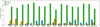 |
Fig. 1 Relative fractions of sources in each class of the labeled set with g-band only, r-band only, or both g- and r-band photometry. |
2.3 Labeled set
The labeled set consists of all the sources used to train and test the classifier, now incorporating 16 subclasses, all of them present in the ZTF stream. The labels were obtained from previous works that studied the sources via spectroscopic and/or photometric analysis. The methodologies utilized to construct labeled sets can be found in more detail in Förster et al. (2021); for this specific labeled set, we gathered labeled sources from the following catalogs: the ASAS-SN catalog of variable stars (ASASSN; Jayasinghe et al. 2018, 2019a,b); CRTS (Drake et al. 2014, 2017); LINEAR catalog of periodic light curves (LINEAR; Palaversa et al. 2013); Gaia Data Release 2 (Gaia DR2; Mowlavi et al. 2018; Rimoldini et al. 2019), the Transient Name Server database (TNS; Gal-Yam 2021), the Roma-BZCAT MultiFrequency Catalog of Blazars (ROMABZCAT; Massaro et al. 2015); the Million Quasars Catalog (MILLIQUAS, version 6.4c, December 2019; Flesch 2019), the New Catalog of Type 1 AGNs (Oh2015; Oh et al. 2015); and the SIMBAD database (Wenger et al. 2000). Additional CV labels were acquired from various catalogs, such as the one by Ritter & Kolb (2003), and were put together by Abril et al. (2020). As for the TDEs, they are the latest to be included in this version and we gathered a sample of 60 of them from TNS Classification reports, The Astronomer’s Telegram (ATel) Classification reports (van Velzen et al. 2021; Hammerstein et al. 2022; Yao et al. 2023). Other sources, such as Ambiguous Nuclear Transients (ANTs) and Extreme Nuclear Transients (ENTs), are too rare to be considered separately, even though their physical origins are believed to be similar to TDEs (Hinkle et al. 2024). Additionally, some of these transients have fainter host galaxies, making host-related features less useful for classification. Including these sources would create a separate category of hostless TDEs within the class. For these reasons, we do not include these sources in the labeled set.
Table 1 displays the number of sources per class in the labeled set, along with their total quantity and corresponding references, while Figure 1 shows the relative fractions of sources with usable light curves in only g, only r, or both g and r. We stress here that the numbers of periodic, stochastic and transient sources have increased by 72%, 89% and 144%, respectively, compared to SS21 for both training and testing. Moreover, the number of sources with only one or two bands available has increased since the last time the model was trained. As a result, we anticipate variations in the model’s performance across certain classes, particularly those with very low numbers in the previous version, such as the SLSNe. As in SS21, we require that sources have ≥6 detections in the g band or ≥6 detections in the r band to compute the 152 previously adopted features as well as the new features of parametric models and color variability features. As in the previous version, we had to deal with a high imbalance, as can be noticed in Table 1; the class with the fewest sources available is now the TDEs.
2.4 Features used by the classifier
We adopt the 152 features included in the previous version (see Tables 2 and 3 of SS21 for a full list). Additionally, we include 24 new features that help to differentiate TDEs from other transients and AGN. In total, the new version of the light curve classifier includes 176 features. As in the previous model, we avoid including features that require a long time to compute. The new features consist of a decay model adjusted to the lc_diff, two features (one per band) decay_1 and decay_2 as parameters of the model, and the chi-squared of this model (preserving the notation _1 or _2 for the g and r band, respectively). Four other features consist of data products that come with the ZTF alert stream. The first is mean_distnr, the mean distance to the nearest source in the reference image PSF-catalog within 30 arcsec (distance measured in pixels). The second is sigma_distnr, the variance of the previous distance. The third and fourth are the parameters chinr and sharpnr that consist of the DAOPHOT (Stetson 1987) chi and sharp parameters of the nearest source in reference image PSF-catalog within 30 arcseconds. Six of the new features are analogous to the Mexican Hat Power Spectrum (MHPS; Arévalo et al. 2012) features calculated in the previous version but adopt a different timescale of 30 to 365 days (more information about this feature is provided in Sect. 3.1 of SS21). The other three new features consist of colors calculated using PanSTARRS1 magnitudes of the nearest reference to the event; these feature colors are sg1-sr1 (g − r band), sr1-si1 (r − i band), si1-sz1(i − z band). From Gomez et al. (2023), we include four new parametric features (two per band), as well as the chi-squared of the model. Finally, the last feature consists of the color variance of the source. We describe the new features below.
Labeled set, displaying the overall hierarchical classes and their subclasses.
2.4.1 Decay model for TDEs
From theoretical arguments and at least some observations, the typical value of the power-law index of the bolometric luminosity in the TDEs decay is thought to scale as D = −5/3 for a full disruption (van Velzen et al. 2021). Having this characteristic decay, a simple model is fitted to the difference magnitude light curve as
![Mathematical equation: $\[m=2.5 ~D ~\log \left[\frac{t-\left(t_d-40\right)}{N}\right],\]$](/articles/aa/full_html/2025/04/aa51951-24/aa51951-24-eq2.png) (1)
(1)
where m is the value of the difference magnitude, N a scale constant to leave the values of the logarithm dimensionless, td the time in which the peak of the light curve occurred and D the decay value of the model that we used as a feature. The model is fitted to ZTF18acnbpmd in Figure 2 and a distribution of the values obtained for transients can be found in Figure 3. The expression t − (td − 40) rescales the time t, originally given as the Modified Julian Date (MJD), to ensure that the peak of the transient light curve is fixed at day 40. This adjustment situates the disruption time, corresponding to day 0, within the rising phase of the light curve. This alignment is particularly useful when the rising part of the transient light curve is not observable.
2.4.2 FLEET features
FLEET is a machine learning algorithm (Gomez et al. 2023) recently optimized to select transient events that are most likely TDEs. Among the features in this classifier, we make use of the computationally efficient parametric model:
![Mathematical equation: $\[m=e^{W~(t-\phi)}-A ~W(t-\phi)+m_0,\]$](/articles/aa/full_html/2025/04/aa51951-24/aa51951-24-eq3.png) (2)
(2)
where m is the difference magnitude, A modifies the decline time relative to the rise time, W is the effective width of the light curve, ϕ is a phase offset relative to the time of the first observation and m0 is the peak magnitude. The model is able to adapt better to the curvature seen in the early phases of TDE light curves, thus complementing the shortcomings of the decay model. The model is applied to ZTF20acitpfz, as shown in Figure 2, and the distribution of the W parameter for the r band within the transient branch is illustrated in Figure 3.
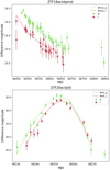 |
Fig. 2 Two example light curves in the g and r band with the following models fitted: the top represents the decay parametric model, and the bottom represents the FLEET parametric model. The fitted models are represented in dashed lines in both plots. |
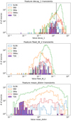 |
Fig. 3 Histograms of the following features for classes in the transient branch in log. The top represents the calculated decays for the g band of all the transients in the labeled set, a black line is plotted to represent the 5/3 usual decay for the TDEs. The middle represents the r band set of data for the W parameter of the FLEET parametric model. The bottom represents the values taken by mean_distnr, showcasing the different distribution of the TDEs compared to the rest of the transients of the labeled set. |
2.4.3 The nr features
Given that TDEs are nuclear events while SN could reside anywhere (predominantly off-nuclear, but occasionally nuclear, dependent on host size and survey spatial resolution), we expect the average TDE position to be consistent with the center of their host galaxy, while SN not necessarily. To use this characteristic, we made use of distnr (nr meaning nearest source in reference image), a ZTF-computed feature available in the alert avro package that corresponds to the pixel distance to the closest in the reference image. For each source, we calculated the mean and the sigma of these values from all previous and current detections. This plays a fundamental role in the early classification of TDEs. The sharpnr and chinr parameters are additional useful features that are present since the first detection, representing the sharp and chi parameters of the DAOPhot best-fit to the nearest source in reference image PSF-catalog within 30”. sharpnr is a goodness-of-fit statistic describing how much broader the actual profile of the object appears than the profile of the PSF; a complete definition of this parameter can be found in the DAOPhot manual. chinr is the estimated goodness-of-fit statistic for the PSF, defined as the ratio of the observed pixel-to-pixel mean absolute deviation from the profile fit to the value expected. Their use was studied by Carrasco-Davis et al. (2021) together with distnr as extra features for the ALeRCE Stamp Classifier.
2.4.4 PanSTARRS1 colors
The alert avro package includes information about PanSTARRS1 cataloged sources. One of the data products provided by the alert is details about the closest PanSTARRS object to every ZTF source. We use the magnitudes in the g, r, i, and z bands from the closest object in the PS1 catalog to the labeled source within 30 arcsec to compute colors.
These colors have proven particularly helpful in classifying stochastic sources, as shown in SS21 to distinguish between AGN, QSO and Blazars. The colors are named sg1-sr1_0 (g − r band), sr1-si1_0 (g − i band) and si1-sz1_0 (i − z band).
2.4.5 Mexican hat power spectra features
Arévalo et al. (2012) proposed a method to compute low-resolution power spectra from data with gaps. Utilized in SS21, this method involves convolving the light curves with a Mexican hat filter: ![Mathematical equation: $\[F(x) \propto\left[1-\frac{x^{2}}{\sigma^{2}}\right] e^{x^{2} / 2 \sigma^{2}}\]$](/articles/aa/full_html/2025/04/aa51951-24/aa51951-24-eq4.png) . Uneven sampling is corrected by convolving a unit-valued mask with the same sampling as the light curve and dividing the convolved light curve by it. In SS21, this method was used to assess the variability amplitude on a characteristic timescale (
. Uneven sampling is corrected by convolving a unit-valued mask with the same sampling as the light curve and dividing the convolved light curve by it. In SS21, this method was used to assess the variability amplitude on a characteristic timescale (![Mathematical equation: $\[t \propto \sigma / \sqrt{2 \pi^{2}}\]$](/articles/aa/full_html/2025/04/aa51951-24/aa51951-24-eq5.png) ) in a given light curve, in order to estimate the light curve variance associated with that timescale; only timescales of 10 and 100 days were assessed in the previous version. Here we compute the light curve variance on timescales of 10, 30, 100, and 365 days for each band, denoted as MHPS_10, MHPS_30, MHPS_100, and MHPS_365, respectively. We also compute ratio features between high and low-frequency variances: MHPS_10_100 and MHPS_30_365.
) in a given light curve, in order to estimate the light curve variance associated with that timescale; only timescales of 10 and 100 days were assessed in the previous version. Here we compute the light curve variance on timescales of 10, 30, 100, and 365 days for each band, denoted as MHPS_10, MHPS_30, MHPS_100, and MHPS_365, respectively. We also compute ratio features between high and low-frequency variances: MHPS_10_100 and MHPS_30_365.
2.4.6 Color variance
Another considered feature is the variance of the color between the g and r bands. TDEs have almost no variation in their color evolution (van Velzen et al. 2011), which distinguishes them from SNe. In particular, TDEs have bluer colors than SNe at similar epochs after the peak. The average variance is calculated using bins of 10-days in width, and is denoted as g-r_var_12.
2.5 Classification algorithm
Table 1 highlights the high imbalance in the labeled set, whereby the QSO class has the largest number of sources and the TDEs the lowest. To account for this imbalance, as in SS21, we use the Imbalanced-learn library, specifically the modified random forest proposed by Chen et al. (2004) that can deal with the imbalanced data classification. We adopt again the hierarchical scheme of SS21, as it currently yields the best results for light curve classification. To train the model and estimate scores, we split the data set several times into training (80%) and test (20%) sets in a stratified fashion, this means that each split preserves the proportion of classes or categories present in the original dataset. By stratifying, we ensure that the distribution of the classes in both the training and test sets mirrors the overall distribution in the entire dataset, preventing any class from being underrepresented or overrepresented in either subset. This approach is particularly important when dealing with imbalanced datasets, where some classes might be less frequent than others.
The two-level classifier approach
SS21 demonstrated (in their Appendix B) that the two-level approach had in fact better performance. This method consisted of a first-level BRF trained to classify broad transient, periodic and stochastic classes, and the second level consists of three BRF for each one of the hierarchical classes and are trained with the corresponding subclasses sources. For instance, the stochastic classifier is trained only with stochastic sources (i.e., QSO, AGN, Blazar, YSO, and CV/Nova). For each source that is tested, each model outputs probabilities of being a certain class: the first level outputs 3 probabilities, and then the final probability of a source being part of a certain subclass is computed by multiplying the first level probability with the corresponding probabilities of the second level. Specifically, we define the top level probabilities, which are Ptop (transient), Ptop (stochastic), and Ptop (periodic). Then within each second level, there are, for instance, Ptransient(SNIa), Ptransient(SNIbc), Ptransient(SNII), Ptransient(SLSN), Ptransient(TDE). So the probability (P) of a source being a TDE is:
![Mathematical equation: $\[P(\mathrm{TDE})=P_{\text {top}}(\text {transient}) * P_{\text {transient}}(\mathrm{TDE}).\]$](/articles/aa/full_html/2025/04/aa51951-24/aa51951-24-eq6.png) (3)
(3)
Using this method, the probabilities of all 16 subclasses add up to 1 for each source, and the source’s final class is the one with the maximum probability1.
3 Results
Following SS21, we used the ShuffleSplit from scikit-learn to randomly generate 20 test and training sets with (80%) and (20%) of the labeled set, respectively. These sets were stratified, meaning that each subclass within the labeled set receives proper representation due to the imbalance. The scores used to estimate the performance of the models are the macro precision, recall, and F1-score. For individual subclasses, the scores are defined as
![Mathematical equation: $\[\operatorname{Precision}_i=\frac{T P_i}{T P_i+F P_i},\]$](/articles/aa/full_html/2025/04/aa51951-24/aa51951-24-eq7.png) (4)
(4)
![Mathematical equation: $\[\operatorname{Recall}_i=\frac{T P_i}{T P_i+F N_i},\]$](/articles/aa/full_html/2025/04/aa51951-24/aa51951-24-eq8.png) (5)
(5)
![Mathematical equation: $\[\mathrm{F1 \text {-score}}_i=2 \times \frac{\operatorname{Precision}_i \times \text {Recall}_i}{\text { Precision}_i+\text {Recall}_i},\]$](/articles/aa/full_html/2025/04/aa51951-24/aa51951-24-eq9.png) (6)
(6)
where T Pi is the number of true positives, F Pi is the number of false positives, and F Ni is the number of false negatives, for a given class i. Macro scores are computed using the macro-averaging method, which treats all classes as equally important even if the set is imbalanced:
![Mathematical equation: $\[\text {Precision}_{\text {macro}}=\frac{1}{n_{c l}} \sum_{i=1}^{n_{c l}} \text {Precision}_i,\]$](/articles/aa/full_html/2025/04/aa51951-24/aa51951-24-eq10.png) (7)
(7)
![Mathematical equation: $\[\operatorname{Recall}_{\text {macro }}=\frac{1}{n_{c l}} \sum_{i=1}^{n_{c l}} \operatorname{Recall}_i,\]$](/articles/aa/full_html/2025/04/aa51951-24/aa51951-24-eq11.png) (8)
(8)
![Mathematical equation: $\[\mathrm{F} 1 \text {-score}_{\text {macro}}=\frac{1}{n_{c l}} \sum_{i=1}^{n_{c l}} \mathrm{F1} \text {-score}_i.\]$](/articles/aa/full_html/2025/04/aa51951-24/aa51951-24-eq12.png) (9)
(9)
here ncl represents the total number of classes.
Table 2 reports the scores obtained for the first and second levels in the classifier for 20 randomly selected train and testing sets. Figures 4 and 5 show the confusion matrices for the first and second level, respectively. The second level matrix contains the final classes predicted for the test set. The scores from the previous version of the classifier, trained with fewer sources and fewer features, are very similar on the first level, it is possible to recover over 99% of the correct labels with 98% precision, as depicted in Table 2. For the second-level confusion matrix, an improvement of ≈2% is obtained in every score in comparison to the scores of SS21 that are present in Table 2. In Figure 5 the percentage of true positives ranges between 57% to 99%.
The confusion in subclasses tends to happen between sources of the same first-level class, for example in this case we have a generalized confusion of all transient classes being predicted as TDEs, but it is not as common to have TDEs predicted as other classes, giving an average precision of 21%, an F1-score of 34% and a recall of 92%; a precision confusion matrix of only transient classes can be found in Figure 6, highlighting the confusion involving this particular class. The false predictions of this subclass are low probability predictions. The results of high probability predictions are discussed in Appendix B where we present some analysis on the sources. Figure B.1 is a confusion matrix that includes only the test sources predicted with ≥50% probability of being that source. It can be observed that when the probability is above a certain threshold, there is very little confusion within the TDE class. The unnormalized confusion matrix on the right in Figure B.2 illustrates the small fraction of TDEs in the test set predicted with a probability of ≥50%. Originally, there were 12 TDEs in the test set, and approximately 8 of them were predicted with a probability of ≥50%. At this threshold, the recall is 100% (No TDEs are being miss-classified) within the test sets, but the completeness as defined in Gomez et al. (2023) (the total number of true positive TDEs divided by the total number of TDEs in the test set) is ≈67%.
Figure 7 displays a plot of TDE probability versus the second-highest probability for all sources predicted as TDEs in the labeled set, using only the transient branch of the classifier. The side histograms illustrate the orthogonal distance of each point to the dashed line; the closer a point is to the dashed line, the more similar the TDE probability is to the second-highest probability. The first histogram (middle panel in Figure 7) shows only the secondary probability of each TDE prediction, while the second histogram (right panel in Figure 7) reveals the actual class of each TDE prediction. This demonstrates that sources classified as TDEs with a second probability close to the TDE probability are most likely SNIa. Because SNIa are more numerous, Ptransient(SNIa) = 0.3 may still be correct ≥50% of the time, just due to the sheer number of SNIa that are detected by ZTF, while TDE predictions start to be reliable after 50% confidence. This is an important measure of the quality of classifications for an unlabeled set, which we analyze in Sect. 3.4. The remaining classes in the transient branch exhibit similar behavior to the TDE class, with the SNIbc class also exhibiting strong contamination from SNIa.
Some modest confusion can also be noticed between QSO, AGN and Blazars. The confusion for the Blazar class has now been reduced in comparison to the previous version by excluding the FSRQ from the training set. The periodic branch subclasses exhibits the same behavior as in the previous version, including the known confusion between the YSO and Periodic-other subclasses.
Mean and standard deviation of the macro-averaged scores of new and previous model.
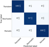 |
Fig. 4 Recall confusion matrix of the top level generated using 20 randomly generated training and testing sets. After predicting the 20 testing sets, a median, and the 5 and 95 percentiles are provided for each class. This matrix is normalized by dividing each row by the total number of objects per class with known labels. We round these percentages to whole numbers. This indicates a high level of accuracy with a low percentage of incorrectly classified sources. |
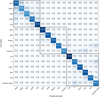 |
Fig. 5 Recall confusion matrix of the bottom-level classifier. It was generated using 20 randomly generated training and testing sets. It showcases the median, 5 and 95 percentile errors for all subclasses. The black squares enclose the confusion matrices for the three distinct bottom-level classifiers. Higher confusion can be seen within the subclasses of the same hierarchic group. |
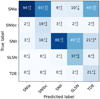 |
Fig. 6 Precision confusion matrix of the transient branch, generated using 20 random training and testing sets. After predicting the 20 testing sets, a median, and the 5 and 95 percentiles are provided for each class. |
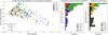 |
Fig. 7 Scatter plot of the sources predicted as TDEs in the labeled set. The x-axis represents the predicted probability of being a TDE, while the y-axis shows the second-highest probability. The dashed gray line represents a 1:1 ratio, where points closer to this line indicate greater uncertainty by the classifier regarding the true class of the source. The middle plot shows the second most probable class labels, while the right plot presents the true class labels of the sources. These histogram plots depict the orthogonal distances of the sources from the dashed line, providing insight into the classifier’s confusion relative to the real classes of the sources. |
3.1 Probability interpretation
The issue of probability uncertainties and systematic displacement in the output of Random Forest models is a well-documented challenge in calibration (Niculescu-Mizil & Caruana 2005; Silva Filho et al. 2023). In this study, the hierarchical structure of the model and the imbalance within the labeled dataset further exacerbate the complexity of the calibration process, assessing the errors on probabilities is a well-known challenge with no straightforward solutions as yet. As such, solving this is not within the scope of this current work. Nonetheless, we assess the reliability of the model’s probability predictions by computing reliability diagrams (Guo et al. 2017) and the expected calibration error (ECE; Pakdaman Naeini et al. 2015) for both the first-level BRF and the transient BRF at the second level. These diagrams provide a quantitative and visual assessment of the alignment between predicted probabilities and true observed frequencies.
To construct the reliability diagrams, we utilized the predicted probabilities obtained from a randomized training and test split. For the first-level classifier, we used Ptop from the entire test set, while for the second-level classifier, we used Ptransient, restricting the analysis to transient sources in the test set. These predicted probabilities were divided into ten bins of equal width (0.1) for their respective reliability diagrams. For each bin, we calculated the positive fraction (PF), defined as the ratio of correctly classified samples to the total number of samples in the bin (equivalent to the micro-averaged precision), as well as the average predicted probability for the bin (referred to as confidence). The reliability diagram plots the PF against the confidence for each bin. When the resulting curve aligns closely with the identity function, it indicates that the predicted probabilities are well-calibrated. Then we measured the gap, defined as the absolute difference between the PF and the confidence within each bin (gap = |PF − confidence|), and we calculated the ECE as
![Mathematical equation: $\[\mathrm{ECE}=\sum_{m=1}^M \frac{N_{\mathrm{bin}}}{N} \text {gap},\]$](/articles/aa/full_html/2025/04/aa51951-24/aa51951-24-eq13.png) (10)
(10)
where N corresponds to the total of samples, Nbin to the total of samples in the probability bin, and M to the total number of probability bins. When the ECE score is close to zero, we can say that the model is well calibrated.
Figure 8 presents the reliability diagrams and the ECE for both the first-level classifier and the transient classifier branch at the second-level. For each bin, we plot the PF (black bar) and respective calibration offset (red region) against the confidence. From the first-level diagram, we observe that the majority of sources are classified with a confidence of ≥90%, while the remaining sources exhibit PF values exceeding their corresponding confidence levels. This trend suggests that the first-level classifier is under-confident in its predictions, but reasonably calibrated. A similar under-confident trend is observed in the transient classifier, but with the majority of the sources being classified between 30% to 50% confidence. Following Equation (3), this implies systematically under-confident overall output probabilities for the transient class. We recommend that users consider these results when applying probability thresholds when using our classifier.
3.2 Feature importance
Table 3 shows the first 30 features that each BRF used to separate between classes. The more informative the feature, the higher the rank. At the top-level classifier, some new features can be noticed in the higher ranks, such as mean_distnr_0 or sharpnr_0; in addition to these features, we find many other features that also dominated the high ranks of importance in SS21, such as the WISE color W1-W2_0, morphological properties of the images (sgscore_Q), the chi-squared of the parametric models such as FLEET or SPM, variability features related with the amplitude of the variability at short and long timescales such as MHPS_30_1, GP_DRW_sigma_2 (in this case, MHPS_30 is a new feature). Some features detect gradual changes in brightness, such as LinearTrend, SPM_tau_rise, and SPM_tau_fall. Finally, as in the previous version, there are features related to transient appearance or disappearance such as positive_fraction_2. For the Transient classifier, we have in the first place the mean_distnr_0 due to its importance in separating a nuclear from a nonnuclear event, and other nr features. SPM, decay and FLEET parametric models are also present in the ranking due to their importance to this classifier specifically. Additional important features include the optical colors at the highest point and for the mean of the light curve, which are measured from the difference image light curves, features that detect smooth increase or decrease of the observed flux (LinearTrend), and features related to the amplitude of the light curve, e.g., the MHPS features. The ranking of the stochastic classifier is mainly dominated by colors, including the new PanSTARRS colors, nr features such as chi and sharp nr, morphology, distance from the Galactic plane (sgscore1_0 and gal_b_Q), amplitude of variability observed at different time scales, such as ExcessVar, SPM_A, Meanvariance, GP_DRW_sigma, and Amplitude, and finally features that are related to the timescale of the variability such as GP_DRW_tau. Finally, the periodic classifier ranking is largely influenced by the Multiband_period feature, as well as various colors (including new ones), features that pertain to the amplitude of the variability (such as delta_mag_fid, Amplitude, ExcessVar, Meanvariance, and GP_DRW_sigma), and features that relate to the timescale of the variations (GP_DRW_tau and IAR_phi).
To assess the usefulness of the new features only for the TDE class, we converted the output of the model into binary values and obtained the feature importance. The results are presented in Figure 9. The analysis revealed that the most important features are those associated with the specific characteristics of this type of source, such as the location within the host galaxies, the canonical decay, and the color variation. Due to the relatively small number of objects in the TDE class, we find that the features identified in the feature importance analysis are sensitive to the selection of sources in the test set. For instance, the features decay_2 and fleet_chi_2 do not appear in Figure 9 for the current iteration. However, in other training iterations, these features can be ranked among the most important, highlighting the variability of feature importance across different subsets of the data. As the number of labeled TDE sources increases, these features are expected to assume more stable positions in the feature importance rankings. Ultimately, we selected the version of Figure 9 because it is the feature ranking used to classify the candidates presented in Section 4.2. Regarding the PS1 colors, most of these features were found to be more significant in other branches of the BRF than in the classification of transients. Nevertheless, we included them because, theoretically, there is a known connection between supernovae (SNe) and their host environments (Hakobyan et al. 2020). Additionally, there is evidence suggesting an overrepresentation of TDEs in post-starburst galaxies, which can potentially be identified through their colors. However, the extent of this overrepresentation remains a topic of ongoing debate.
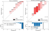 |
Fig. 8 Reliability diagrams for the first-level classifier and the second-level transient classifier. The positive fraction (PF) is shown in black, and the respective calibration offset is indicated in red, both plotted against the confidence. The red shading for the latter reflects the density of sources within the corresponding probability bin, with darker shades indicating higher numbers of samples. The identity function is included as a reference. The bottom panels of the diagrams display the source count for each confidence bin. |
Top 30 most important features for each branch of the classifier.
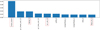 |
Fig. 9 Feature importance for the TDE class. Features enclosed by red rectangles are newly introduced to the lc_classifier. |
3.3 Evolution of TDE recall
A critical goal of transient classification is to facilitate fast, efficient, and useful confirmation and follow-up campaigns. In this sense, the ability of a classifier to make accurate and precise classification based on early or incomplete light curves is highly desirable. Here we investigate the ability of our new lc_classifier to classify both top-level transients and bottom-level transient subclasses as a function of time. In the latter, we focus on the TDE subclass, as that is the theme of this investigation, but note that our results are generally relevant to the entire transient taxonomy.
To analyze the recall of TDEs, for early and late classification, we recalculated the features for these sources in different time frames varying from 15 to 120 days since their discovery, then we predict them. The results on TDE recall are summarized in Figure 10 we tested classifying using all the features, then only g, only r and only nr. The top level gives us an ≈60% recall on the TDE class as a generic transient in only 15 days, while at 40 days a 100%. On the bottom level, at 15 days we observe ≈60% recall if we follow the black curve that includes all the features, while at 30 days the recall goes up to 80% in the case of occupying all the features available. Using only the nr features, which are available since the first detection, we find ≈40% recall for this subclass on the first level and ≈45% on the second. It is important to note that LC features are only calculated after ≥6 detections, which may not occur within the first 15 days. In particular, only 13% of the TDEs have ≥6 detections at 15 days, and while for the rest the classification is based solely on the nr and PanSTARRS color features. In Figure 11, we show the evolution of the transient branch (recall) confusion matrices at 15, 40 and 100 days. We can see that the TDE class (and in fact most classes) emerges as relatively well classified (lower confusion and smaller errors) only after ~40 days.
Referring back to the fraction of sources used for training the model in Figure 1, it is evident that there are no TDE sources with only r-band observations. Figure 10 provides insight into the model’s performance when classifying TDE candidates based solely on r-band detections. The results highlight that the TDE recall is significantly lower when one of the bands is unavailable, underscoring the importance of color variability features in the transient branch of our classifier. Therefore, as a precaution, it is recommended that both bands be available to ensure reliable second-level transient classifications.
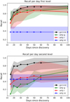 |
Fig. 10 Recall per day for the TDE subclass on the first level (top) and the second level (bottom). The colored symbols, curves, and shaded regions indicate the median and 5–95 quantile ranges of recall, depending on whether the model was trained with all features (g + r + nr; black and gray), only g-band features (green), only r-band features (red), or only nr features (blue). |
3.4 Unlabeled set tests
To examine the results of the classifier, we investigate the properties of the unlabeled dataset, several tests have been conducted using ALeRCE’s database unlabeled set, which consists of approximately 1.7 million sources.
Predicted distributions for the unlabeled set are shown in Figure 12. As in SS21, periodic sources comprise a majority, while transient classes represent the smallest fraction. Notably, the SLSN class appears to be strongly overrepresented compared to expectations, although most sources labeled as SLSN have relatively weak probability predictions. A similar effect is seen for the TDE class in Figure 13, which presents the top and bottom level classifier probability distributions for TDEs2; the probability distributions for the other transient subclasses remain unchanged compared to SS21. When we consider probabilities above 50%, the predicted distribution, shown in the bottom of Figure 12, aligns more closely with the observed ratios of confirmed astrophysical SNe (e.g., Li et al. 2011). However, it still overestimates the occurrence of SLSNe and TDEs. Nonetheless, the discovery rates of these last two classes are increasing with advancements in astronomical surveys. A scatter plot of the unlabeled sources predicted as TDEs by the transient branch can be found in Figure 14. This figure only represents the probability distributions output by the BRF trained on the transient class (Ptransient), which has probabilities limited to a minimum of 20% per class, given that there are 5 classes in this branch. It shows a different distribution of probabilities compared to Figure 13, which represents the overall probabilities of both levels of the classifier as stated in Equation (3). The unlabeled objects in Figure 14 show a similar distribution to the labeled set plotted in Figure 7, in particular for the histogram of orthogonal distances of the second highest probability predictions; this implies that the majority of the sources predicted as TDEs with probabilities close to the 1:1 line have a high chance of being SNe Ia.
To test the degree to which the entire unlabeled sample from the lc_classifier agree with astrophysical expectations, we plot the galactic latitude (gal_b) vs g − r mean color (g-r_mean) for extragalactic objects (QSO, AGN, Blazars, and transients) in Figure 15, as was shown in SS21. The highest probability objects lie furthest from the galactic plane, and have colors most typical of extragalactic objects. We can also notice enhanced reddening among objects closer to the galactic plane, due to dust attenuation. These results are identical to those of SS21, implying that the new features have not drastically changed the general performance of the lc_classifier.
As seen in Table 3, the new Decay, mean_distnr, and FLEET features are among the top ones of the transient branch. In Figure 16, a relation is seen between the mean_distnr feature and the probability of the source being part of particular predicted classes. The TDEs especially seem to show higher probabilities for lower distances to the center of the host galaxies.
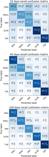 |
Fig. 11 Recall confusion matrices of the transient branch subclasses for sources at 15 (top), 40 (middle), and 100 (bottom) days after detection. |
Comparison of macro-averaged scores for different model versions.
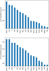 |
Fig. 12 Predicted source distribution from the lc_classifier for the full (top) and ≥50% probability (bottom) samples of unlabled sources. |
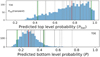 |
Fig. 13 Histograms displaying normalized probability distributions for the top and bottom level probabilities for the TDE candidates of the unlabeled set. Red lines denote the median probability for each class, green lines show the 5 and 95 percentiles, and dashed gray lines show the predictions for a sample of spectroscopically confirmed TDEs. |
4 Discussions
4.1 Comparison with other works
4.1.1 SS21 model comparison
In order to isolate the effects of the increased training set size from those of the new features, we trained a model using the same 20 randomly generated training and test sets as in SS21, but restricted it to the original 152 features. In Table 4 and Figure 17, we present the performance of this model. Comparing scores and feature importance in both models, we see an improvement of ≈1% in all macro scores. Comparing these to the new lc_classifier, we see small improvements to the stochastic and periodic branches, but mainly the new features (e.g., decay, nr) improve the transient classifications. Comparing confusion matrices of the models that use the new (Figure 5) or only previous (Figure 17) features, it is noticeable that the latter has more generalized confusion between other classes and the newly introduced TDEs, with many TDEs being classified as SLSN and SNII; this is not the case for the model using the new features, which yields 92% recall for TDEs. The benefit of the new features is noticeable across all the subclasses of the transient branch. From this, we conclude that as more classes are added and the diversity of the training set is increased, the more novel features from the light curves must be provided to achieve good performance.
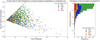 |
Fig. 14 Scatter plot illustrating sources predicted as TDEs by the transient branch within the unlabeled dataset. The x-axis denotes the predicted probability of being a TDE, while the y-axis indicates the second-highest predicted probability. The dashed gray line signifies a 1:1 ratio, where points closer to this line suggest greater uncertainty by the classifier about the true class of the source. Additionally, the histogram shows the distribution of the second-highest probability class labels relative to the orthogonal distances from the dashed line, highlighting the classifier’s confusion concerning the actual classes of the sources. |
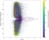 |
Fig. 15 Galactic latitude versus g − rmean for extragalactic candidates (QSO, AGN, blazar, SNIa, SNIbc, SNII, SLSN, and TDE classes). The colorbar at right denotes the bottom-level probability. As expected, the majority of the high probability extragalactic objects are located outside the Galactic plane. |
4.1.2 FLEET model comparison
FLEET is a random forest machine-learning algorithm recently adapted to classify TDEs. It uses as a training set spectroscopically confirmed transients from TNS, similar to the transient branch of our classifier. However, a crucial difference between their labeled sets and the one gathered in this work is that they only use 45 TDEs for training. Thus to have a completely fair comparison with their model, we should ideally use the same training set. They optimized their model to a set of 14 features; apart from the ones we implemented from their early fitting model, the majority of their features have a counterpart in our model. To address the imbalance of their labeled set, they utilize Synthetic Minority Oversampling Technique (SMOTE; Chawla et al. 2002) and evaluate performance through k-fold cross-validation. For the TDE classification, they binarized the output of their model and provide two classifiers, a rapid one trained on 20 days of photometry and a late-time classifier trained on 40 days of data. For events with P(TDE) > 0.5, the rapid classifier has and a 30% purity with 40% completeness3; ≈50% purity and ≈20% completeness can be achieved by the P(TDE) > 0.8 threshold. The late-time classifier achieves completeness of ≈30% for transients with P(TDE) > 0.8, but with a higher peak purity of ≈90%. Given the similarities, we compare their late classification performance to the 40-day confusion matrices of Figure 11. Their model uses binarized statistics, making direct comparison of threshold probabilities not straightforward, as we subsequently discuss later in this section. For a threshold of P(TDE) > 0.5 in our classifier, the 40-day confusion matrix in Figure 11 shows a 100% recall, which corresponds to approximately 33% completeness and 82% purity. These scores are comparable to those achieved by their late-time classifier with P(TDE) > 0.8. For our late-time classification, which corresponds to a model trained with full light curves and analyzed using the probability threshold discussed in Appendix B, we achieve approximately 70% purity and 67% completeness.
As mentioned earlier, some tentative sources predicted by FLEET are also predicted by our classifier as TDEs; these sources can be found in Table 5. The lower probabilities assigned by the lc_classifier, compared to FLEET, likely stem from its binary classification approach (and the under-confidence of our classifier, as discussed in Section 3.1). This approach may down-play degeneracies with other transient classes, resulting in the “missing” probabilities being distributed across numerous other branches or subclasses. The majority of candidates that our classifier did not predict were absent from ALeRCE’s database. However, for the specific case of ZTF21aakfqwq (2021crk), this source is included in our labeled set. Additionally, only two sources that we predicted with a probability of ≥50% overlap with their predictions. One of these, ZTF21 aasztrl (2021iqs), was visually inspected and determined not to be a TDE due to its late color evolution. The other, ZTF20aaqppwh (2020dxw), has been analyzed to be a likely TDE.
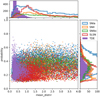 |
Fig. 16 Scatter plot of mean_distnr feature versus predicted probabilities; the higher probabilities of the TDE predictions align with lower mean_distnr values. |
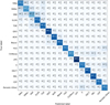 |
Fig. 17 Matrix corresponding to the bottom-level classifiers trained with only the 152 features of SS21 and the labeled set gathered in this work. It was generated using 20 randomly generated training and testing sets, it showcases the median, the 5 and 95 percentile of all subclasses. For the most part, the matrix looks diagonal; however some confusion can be seen especially within the transient subclasses, due to the lack of new features. |
4.1.3 tdescore model comparison
The other ML-based algorithm for TDE classification is tdescore, which adopts XGBoost specifically trained with a sample of uniform light curves that passed through a selection process, the algorithm is fully binary and classifies only TDEs. Their labeled set consists of solely nuclear events comprised of 2153 AGN, 106 CCSNe (Core Collapse SNe), 427 SNIa, 3 variable stars and 55 TDEs. They adopt a set of 27 features, the majority of which have counterparts in our classifier. The key features not shared are the original Gaussian model they implemented and SALT2 (Guy et al. 2007) features. In the tdescore model, the features with the strongest impact are the WISE colors (related to the dominance of AGN in their labeled set), the distance to the host galaxy, the color variation with time, and the color at the peak. We note that the FLEET model also incorporates the distance to host galaxy and the color at peak, while they replace the color variation feature with the color at 40 days after the peak. For the imbalanced set problem, tdescore also makes use of SMOTE. The final performance of the model yielded a recall of ≈77% and a ≈80% precision. In our classifier, the TDE class shows confusion with other transient subclasses apart from AGN and SNIa. Additionally, the SNIa training set included in our model is much larger and exhibits more diversity than that of tdescore. These differences help to explain the much lower precision yet better recall of our lc_classifier model.
Comparison of probabilities for the unlabeled TDEs predicted by FLEET with ≥50% probability and our lc_classifier.
4.1.4 NEEDLE comparison
NEEDLE (Sheng et al. 2024) is a convolutional neural network (CNN) + dense neural network that is trained to distinguish between SNe (SNIa, Core collapse and interacting SNe), SLSNe (hydrogen-poor SLSNe Type I) and TDEs. Their sample consists of over 5000 SNe, 87 SLSNe and 64 TDEs. The CNN architecture of the model is inspired in Carrasco-Davis et al. (2021) stamp_classifier while some of the features of the metadata have a close counterpart to the features in our classifier such as the separation with the host galaxy or the host galaxy colors. As the case of FLEET and tdescore, the different number of classes between our classifiers make the threshold comparison not straightforward. For TDE predictions in a threshold P(class) ≥ 0.75 and a balanced test set consistent of 15 sources per class, they obtain completeness of 50.4% and purity 92.3%. This statistics refer to a different test set than hours, a more fair comparison is the statistics depicted on their Figure 11(b,c) which correspond to a threshold of P(class) ≥ 0.75 on a full test set, this is more similar to our P(class) ≥ 0.5 threshold in which we obtain more completeness and purity. A more direct comparison could be made if we compared recall confusion matrices between our predictions of the full test set without thresholds, however these results are not explicit in Sheng et al. (2024) and even if the model’s performance without thresholds were presented, the differences in the labeled sets would significantly impact the purity of the TDE predictions. This is because their training set contained a higher number of SNIa, which, as demonstrated in previous sections, are the primary contaminants of the TDE class.
Following on their performance, they presented predictions on an untouched validation set, similar to what we subsequently present in the following section. Among the candidates they identified, we concur on ZTF23aadcbay, ZTF23aamsetv, and ZTF23abaujuy, which are TDEs from 2023. In contrast, our validation set primarily consists of older sources classified as TDEs in the Transient Name Server (TNS). Based on their performance, they presented predictions on an untouched validation set, similar to what we subsequently present in the following section. Among the candidates they identified, we concur on ZTF23aadcbay and ZTF23aamsetv which are TDEs from 2023. In contrast, our validation set primarily consists of older sources classified as TDEs in TNS, this means that none of the other sources predicted by them were in our unlabeled set at the time.
4.2 TDE candidates from the unlabeled set
From the probabilities outputted by the model, we gathered a sample of 56 sources with ≥50% probability of being a TDE, listed in Table A.1. A team of experts visually inspected the light curves and metadata, and found that a large minority showed good promise. Specifically, among this sample, seven are already classified as TDEs in TNS (they were not used in the labeled set), demonstrating the efficacy of the classifier. An additional 15 were considered likely TDEs by experts, based on characteristics such as their blue colors, little color variation and typical “TDE-like” timescales. From this analysis, 41% of the sources with ≥50% probability have a high chance of being a TDE. The rest of the predicted sources are under observation, between them there are sources also predicted by FLEET to be TDEs; this set can be found in Table 5.
Our model’s TDE predictions are limited to the (arguably) ‘standard’ TDEs in the labeled set. Special cases such as TDEs occurring in AGN will most likely be predicted as AGN, while other special cases such as partial TDEs (pTDEs) are also not considered among the predictions because they are not part of the training set. Examining the 7 predicted TDEs in Figure 21 that are already confirmed in TNS, they all share similar characteristics. The majority of the alert detections occur well after peak, and thus appear consistent with the decay feature expectation, but show more diversity at early times, potentially making early classification difficult. Another noticeable feature in common is the low color variability. A special case is ZTF22aafvrnw, which is double-peaked. Including this kind of source in a future training set may prove useful for the differentiation of TDEs and pTDEs. Additional sources classified as TDEs in TNS were also identified by the classifier, albeit with lower probabilities. As shown in Figure 13, the spectroscopically confirmed TDEs are predicted with probabilities ranging from approximately 20% to 74%. Most of the candidates in Table A.1 that lack spectroscopic confirmation or classification in TNS are too faint now to target with confirmation spectroscopy. One possibility remaining to confirm their TDE classification may be to search for late radio emissions (Cendes et al. 2024; Anumarlapudi et al. 2024; Zhuang et al. 2025). We expect to use this classifier in future works to find younger TDE candidates and obtain late radio and spectroscopic confirmation.
Another, albeit indirect, way to test our TDE predictions is to assess the properties of their host galaxies, such as stellar mass, log(Mstellar/M⊙). For this, we crossmatch our candidates to the Sloan Digital Sky Survey data release 8 (SDSS DR8; Aihara et al. 2011) catalog specifically with the data provided by the MPA-JHU group based on the methods of Brinchmann et al. (2004), Kauffmann et al. (2003) and Tremonti et al. (2004); 350 sources had a close counterpart. We plot the distribution of host galaxy stellar masses in Figure 18, and use the conversion of Reines & Volonteri (2015) to estimate central massive black hole masses. We found that the majority of the inferred black hole masses for the predicted TDEs fall within the expected range of 105 to 108 solar masses (Rees 1988). However, there is a noticeable difference in the distribution of predicted sources compared to the labeled ones, with most of the predicted sources having masses above 107.5 solar masses. Unfortunately, we only matched two high-probability sources, neither of which exceed the 107.5 mark.
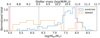 |
Fig. 18 Histogram of the host black hole (BH) masses (bottom x-axis) and stellar masses (top x-axis) of 350 predicted sources and 33 TDEs from the labeled set, each associated with a host galaxy. These masses were calculated using the stellar masses of the host galaxies (using the relation in Reines & Volonteri 2015), as provided by the MPA-JHU group and included in SDSS DR8 (Aihara et al. 2011). The red dashed lines indicate the theoretical mass range within which a TDE is expected to occur. The dashed gray lines mark the locations of ZTF18aaowtgn and ZTF22aajnyhg, which are among our 56 TDE candidates with a probability above 50%. |
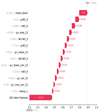 |
Fig. 19 Waterfall plot of ZTF22aaddwbo. Color related features seem to dominate the importance for the classification of this source. Other key features are the mean_distnr, the color variation and the decay. |
4.2.1 Relative feature importance
To examine the relative importance of the TDE features in the BRF algorithm for individual TDE, we carry out an analysis of the SHapley Additive exPlanations values (SHAP values, Lundberg & Lee 2017). To do this, we retrain the transient branch with the sources we want to analyze. A score is assigned to each feature for each source. This score sums up to one across all features and subclasses. Each source starts with a base value of 0.2 for each subclass, denoting an equal initial likelihood among the five transient subclasses. Each feature provides some incremental change to the scores of each subclass, depending on the value of that feature. As an example, we show a waterfall plot of the contributions of each feature to the final score of the source ZTF22aaddwbo (which is present in Table A.1) for being a TDE in Figure 19. We see crude agreement with the general top features in Figure 9, but the order can vary from source to source.
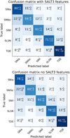 |
Fig. 20 Recall confusion matrices for the transient branch with (top) and without (bottom) the inclusion of SALT3 features. |
4.2.2 Future developments
Given the nature of the new features presented here, we expect them to be relevant and influential in many upcoming time-domain surveys such as BlackGEM (Groot et al. 2022), La Silla Schmidt Southern Survey4, and Rubin’s LSST on the ground, and Ultraviolet Transient Astronomy Satellite (ULTRASAT5) and Ultraviolet Explorer (UVEx6) in orbit. TDEs are known to separate from other transients in the u, NUV, and FUV bands, so including or developing features for these bands (primarily color-related features) is likely to improve the precision and recall of the class (van Velzen et al. 2020), effectively breaking the degeneracy between transients in the early days of observation. For instance, with the advent of LSST, which will include six (ugrizy) filters, we anticipate that the availability of these new bands will play a pivotal role in distinguishing TDEs from other SNe classes. Unlike the cadence of LSST, which is unlikely to serve as the main discriminator, we envision that color features derived from the extended set of bands will become the most critical factors for the early classification of TDEs. Similar advantages are expected when additional filters are available just by reproducing and/or reinforcing the already existing features, as demonstrated in Figure 10 or in SS21; notably, the presence of both g and r bands in the classification shows improved performance. Additionally, features that leverage information from both filters simultaneously have proven to be useful in the classification of transients, such as the SALT3 model features (Kenworthy et al. 2021); the latter features were implemented in the tdescore model and ranked high in their feature importance. These parameters, and in particular the chi-squared of the model, were tested in this work but ultimately were not included due to their high computational cost to run (more than 1 second per light curve). A comparison of the recall confusion matrices of the transient branch including or not these features can be found in Figure 20. The SALT3 model is specially intended to fit SNIa light curves, and hence the goal of including such model features is to better identify and separate the SNIa subclass from other subclasses, as SNIa’s are the main contaminants across all transient branch subclasses. As illustrated in Figure 20, incorporating SALT3 features enhances the classification accuracy for our training sample by improving the recall of the SNIa subclass and reducing confusion with TDEs. However, this improvement is not as significant and, as previously noted, implementing the set of SALT3 features is time-consuming, which contradicts our objective of rapid classification. Therefore, we did not pursue it further.
At the same time, we expect some fraction of the predicted TDEs in Table A.1 to be confirmed either directly through late-time spectroscopy or indirectly from host galaxy redshifts. This will naturally increase the number and diversity of confirmed TDEs available for our training and testing sets.
 |
Fig. 21 ZTF g- and r-band light curves for the seven predicted TDE candidates with ≥50% probability that are already classified as TDEs in TNS and not included in our labeled set. |
5 Conclusions
In this paper, we present an updated version of the ALeRCE light curve classifier presented in SS21. A two-level hierarchical model based on BRF algorithms with 176 features, 24 of which are new compared to the previous version. The majority of the new features focus on improving the transient branch of the classifer, and in particular target special characteristics of the TDE subclass, such as their canonical smooth power-law decay or their lack of color variability. For the new TDE subclass, we obtained a recall of ≈92% and a precision of ≈21%, while every macro score gained ≈2% compared to the model in SS21, largely due to the substantially expanded training sets (increases of ~70–140%). Our model, compared to other models in the literature, demonstrates greater diversity within the labeled set and provides a more detailed analysis of confusion among subclasses. This comprehensive approach allows for a more in-depth comparison with various transient and stochastic subclasses. While our model achieves better recall, it exhibits lower precision, primarily due to the increased diversity of our labeled set, which includes a large sample of SNIa and other classes of stochastic variable sources. This inclusion impacts performance metrics relative to other classification models but trains the classifier to reflect real discovery fractions more accurately, providing a robust and realistic performance evaluation without relying on artificial data generation methods. If in the testing process, we cut out the sources with probabilities lower than 50% of being that source, after 20 randomly selected training and test sets we get approximately 70% precision, a 100% recall and ≈67% completeness. Splitting our TDE classifications into all (i.e., the highest probability class is TDE, but Ptransient(TDE) can be well below 50%) and highly secure (Ptransient(TDE) > 50%), we find ~2700 and 56 in our unlabeled set, respectively. Among the 40 TDEs in TNS and observed by ZTF, yet not in our labeled set, we recover 19 in all the classifications and 7 in our highly secure subsample.
The classifier can identify TDEs that were not included in the labeled set, a capability crucial for predicting the large number of samples expected from LSST photometry. Currently, none of the Ptransient(TDE) > 50% subsample are still active, but we anticipate uncovering more in future unlabeled set predictions. By reclassifying an updated unlabeled set on March 2024, our classifier predicted two interesting sources as TDEs. The first one, ZTF22abzajwl, exhibited characteristics of a TDE in 2023 and experienced another rebrightening in February 2024. The second, ZTF23aaazdag, is a very long transient, first detected in 2023 and lasting approximately 519 days. Given the statistics of early classification, we expect considerable confusion at around 15 days due to the low number of features calculated with fewer than six detections. However, by the 40 days mark, we find the performance comparable to that of a full light curve. As a followup to this research, with the advent of upcoming and ongoing time-domain imaging surveys such as LS4, BlackGEM (Groot et al. 2022) and eventually LSST and along with the Chilean AGN/Galaxy Extragalactic Survey (4MOST-ChANGES; Bauer et al. 2023), The Time-Domain Extragalactic Survey (4MOST-TiDES; Swann et al. 2019) and Son Of X-Shooter (SOXS; Schipani et al. 2024) for spectroscopic confirmation, we aim to establish a relationship between various spectral classes of TDEs and their respective light curves. To achieve this, we need to identify new TDEs within the ZTF alert system. This relationship will facilitate the development of a classifier and pipeline capable of identifying various TDE subclasses.
Acknowledgements
We gratefully acknowledge funding from ANID grants: Millennium Science Initiative Program #ICN12_009 and AIM23-0001 (MPH, FEB, AMMA, LHG, FF, MC); CATA-BASAL #FB210003 (FEB, CR, MC); BASAL #FB210005 (AMMA); FONDECYT Iniciación #11241477 (LHG) and FONDECYT Regular #1200495 (FEB), #1211374 (PH, LHG), #1230345 (CR), #1231637 (MC), #1231877 (GC, LHG), and #1241005 (FEB)
Appendix A TDE candidates
56 TDE candidates with probabilities of ≥50%.
Appendix B 50% probability threshold predictions
Figure B.1 provides a summary of the recall confusion matrix for sources with a probability of 50% or higher in our labeled set. Compared to the confusion matrix in Figure 5, each subclass exhibits higher recall and lower confusion. This improvement is also evident in the scores presented in Table B.1, which are significantly higher for the ≥50% probability sample.
An analysis of the precision within the transient branch on Figure B.2 reveals that, for the ≥50% probability sample, the TDE class has achieved a precision of approximately 70%, with minimal contamination from SNIa in the labeled set; the primary contaminant is now SNII. Table A.1 confirms that one of the spectroscopically classified contaminants is an SNII. This absence of SNIa contamination in the confusion matrix, however, might not hold for predictions in Table A.1. Given the large numbers in the unlabeled set predictions, a majority of them are likely to be SNIa.
Mean and standard deviation of the macro-averaged scores for the bottom level classifier
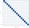 |
Fig. B.1 Recall confusion matrix of the bottom-level classifiers trained with the 176 features and the labeled set gathered in this work, only displaying the test set sources predicted with ≥50% probability. Generated using 20 random training and testing sets, we display a median, and the 5 and 95 percentiles for each class predictions. |
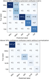 |
Fig. B.2 Precision (top) and Unnormalized (bottom) confusion matrices of the transient branch classifier, trained with the 176 features and only displaying the test set sources predicted with ≥50% probability. Generated using 20 random training and testing sets, we display a median, and the 5 and 95 percentiles for each class predictions. |
References
- Abril, J., Schmidtobreick, L., Ederoclite, A., & López-Sanjuan, C. 2020, MNRAS, 492, L40 [NASA ADS] [CrossRef] [Google Scholar]
- Aihara, H., Allende Prieto, C., An, D., et al. 2011, ApJS, 193, 29 [NASA ADS] [CrossRef] [Google Scholar]
- Anumarlapudi, A., Dobie, D., Kaplan, D. L., et al. 2024, ApJ, 974, 241 [Google Scholar]
- Arévalo, P., Churazov, E., Zhuravleva, I., Hernández-Monteagudo, C., & Revnivtsev, M. 2012, MNRAS, 426, 1793 [CrossRef] [Google Scholar]
- Bauer, F. E., Lira, P., Anguita, T., et al. 2023, The Messenger, 190, 34 [NASA ADS] [Google Scholar]
- Bellm, E. C., Kulkarni, S. R., Graham, M. J., et al. 2019, PASP, 131, 018002 [Google Scholar]
- Brinchmann, J., Charlot, S., White, S. D. M., et al. 2004, MNRAS, 351, 1151 [Google Scholar]
- Carrasco-Davis, R., Reyes, E., Valenzuela, C., et al. 2021, AJ, 162, 231 [NASA ADS] [CrossRef] [Google Scholar]
- Catelan, M. 2023, Mem. Soc. Astron. Ital., 94, 56 [Google Scholar]
- Cendes, Y., Berger, E., Alexander, K. D., et al. 2024, ApJ, 971, 185 [NASA ADS] [CrossRef] [Google Scholar]
- Chawla, N., Bowyer, K., Hall, L., & Kegelmeyer, W. 2002, J. Artif. Intell. Res., 16, 321 [CrossRef] [Google Scholar]
- Chen, C., Liaw, A., & Breiman, L. 2004, Using Random Forest to Learn Imbalanced Data, Report Number 666, University of California, Berkeley, USA [Google Scholar]
- Dekany, R., Smith, R. M., Belicki, J., et al. 2016, SPIE Conf. Ser., 9908, 99085M [Google Scholar]
- Drake, A. J., Graham, M. J., Djorgovski, S. G., et al. 2014, ApJS, 213, 9 [Google Scholar]
- Drake, A. J., Djorgovski, S. G., Catelan, M., et al. 2017, MNRAS, 469, 3688 [NASA ADS] [CrossRef] [Google Scholar]
- Evans, C. R., & Kochanek, C. S. 1989, ApJ, 346, L13 [Google Scholar]
- Flesch, E. W. 2019, arXiv e-prints [arXiv:1912.05614] [Google Scholar]
- Förster, F., Cabrera-Vives, G., Castillo-Navarrete, E., et al. 2021, AJ, 161, 242 [CrossRef] [Google Scholar]
- Gal-Yam, A. 2021, in American Astronomical Society Meeting Abstracts, 237, 423.05 [Google Scholar]
- Gomez, S., Villar, V. A., Berger, E., et al. 2023, ApJ, 949, 113 [Google Scholar]
- Groot, P. J., Bloemen, S., Vreeswijk, P. M., et al. 2022, SPIE Conf. Ser., 12182, 121821V [NASA ADS] [Google Scholar]
- Guo, C., Pleiss, G., Sun, Y., & Weinberger, K. Q. 2017, in Proceedings of Machine Learning Research, 70, Proceedings of the 34th International Conference on Machine Learning, eds. D. Precup, & Y. W. Teh (PMLR), 1321 [Google Scholar]
- Guy, J., Astier, P., Baumont, S., et al. 2007, A&A, 466, 11 [NASA ADS] [CrossRef] [EDP Sciences] [Google Scholar]
- Hakobyan, A. A., Barkhudaryan, L. V., Karapetyan, A. G., et al. 2020, MNRAS, 499, 1424 [NASA ADS] [CrossRef] [Google Scholar]
- Hammerstein, E., van Velzen, S., Gezari, S., et al. 2022, ApJ, 942, 9 [Google Scholar]
- Hills, J. G. 1975, Nature, 254, 295 [Google Scholar]
- Hinkle, J. T., Shappee, B. J., Auchettl, K., et al. 2024, arXiv e-prints [arXiv:2405.08855] [Google Scholar]
- Ivezić, Ž., Kahn, S. M., Tyson, J. A., et al. 2019, ApJ, 873, 111 [Google Scholar]
- Jayasinghe, T., Kochanek, C. S., Stanek, K. Z., et al. 2018, MNRAS, 477, 3145 [Google Scholar]
- Jayasinghe, T., Stanek, K. Z., Kochanek, C. S., et al. 2019a, MNRAS, 486, 1907 [NASA ADS] [Google Scholar]
- Jayasinghe, T., Stanek, K. Z., Kochanek, C. S., et al. 2019b, MNRAS, 491, 13 [Google Scholar]
- Kauffmann, G., Heckman, T. M., White, S. D. M., et al. 2003, MNRAS, 341, 33 [Google Scholar]
- Kenworthy, W. D., Jones, D. O., Dai, M., et al. 2021, ApJ, 923, 265 [NASA ADS] [CrossRef] [Google Scholar]
- Li, W., Leaman, J., Chornock, R., et al. 2011, MNRAS, 412, 1441 [NASA ADS] [CrossRef] [Google Scholar]
- Lundberg, S., & Lee, S.-I. 2017, arXiv e-prints [arXiv:1705.07874] [Google Scholar]
- Massaro, E., Maselli, A., Leto, C., et al. 2015, Astrophys. Space Sci., 357 [Google Scholar]
- Masterson, M., De, K., Panagiotou, C., et al. 2024, ApJ, 961, 211 [NASA ADS] [CrossRef] [Google Scholar]
- Mowlavi, Lecoeur-Taïbi, I., Lebzelter, T., et al. 2018, A&A, 618, A58 [NASA ADS] [CrossRef] [EDP Sciences] [Google Scholar]
- Niculescu-Mizil, A., & Caruana, R. 2005, in Proceedings of the 22nd International Conference on Machine Learning, ICML ’05 (New York, NY, USA: Association for Computing Machinery), 625 [Google Scholar]
- Oh, K., Yi, S. K., Schawinski, K., et al. 2015, ApJS, 219, 1 [Google Scholar]
- Pakdaman Naeini, M., Cooper, G., & Hauskrecht, M. 2015, Proc. AAAI Conf. Artif. Intell., 29 [Google Scholar]
- Palaversa, L., Željko Ivezić, Eyer, L., et al. 2013, AJ, 146, 101 [CrossRef] [Google Scholar]
- Phinney, E. S. 1989, in The Center of the Galaxy, 136, ed. M. Morris, 543 [CrossRef] [Google Scholar]
- Rees, M. J. 1988, Nature, 333, 523 [Google Scholar]
- Reines, A. E., & Volonteri, M. 2015, ApJ, 813, 82 [NASA ADS] [CrossRef] [Google Scholar]
- Rimoldini, Holl, B., Audard, M., et al. 2019, A&A, 625, A97 [NASA ADS] [CrossRef] [EDP Sciences] [Google Scholar]
- Ritter, H., & Kolb, U. 2003, A&A, 404, 301 [NASA ADS] [CrossRef] [EDP Sciences] [Google Scholar]
- Sánchez-Sáez, P., Reyes, I., Valenzuela, C., et al. 2021, AJ, 161, 141 [CrossRef] [Google Scholar]
- Schipani, P., Campana, S., Claudi, R., et al. 2024, arXiv e-prints [arXiv:2407.17241] [Google Scholar]
- Sheng, X., Nicholl, M., Smith, K. W., et al. 2024, MNRAS, 531, 2474 [Google Scholar]
- Silva Filho, T., Song, H., Perello-Nieto, M., et al. 2023, Mach. Learn., 112, 3211 [CrossRef] [Google Scholar]
- Stein, R., Mahabal, A., Reusch, S., et al. 2024, ApJ, 965, L14 [Google Scholar]
- Stetson, P. B. 1987, PASP, 99, 191 [Google Scholar]
- Swann, E., Sullivan, M., Carrick, J., et al. 2019, arXiv e-prints [arXiv:1903.02476] [Google Scholar]
- Tremonti, C. A., Heckman, T. M., Kauffmann, G., et al. 2004, ApJ, 613, 898 [Google Scholar]
- Ulmer, A. 1999, ApJ, 514, 180 [Google Scholar]
- van Velzen, S., Farrar, G. R., Gezari, S., et al. 2011, ApJ, 741, 73 [Google Scholar]
- van Velzen, S., Gezari, S., Hammerstein, E., et al. 2021, ApJ, 908, 4 [NASA ADS] [CrossRef] [Google Scholar]
- van Velzen, S., Holoien, T. W. S., Onori, F., Hung, T., & Arcavi, I. 2020, Space Sci. Rev., 216, 124 [CrossRef] [Google Scholar]
- Wenger, M., Ochsenbein, F., Egret, D., et al. 2000, A&AS, 143 [Google Scholar]
- Yao, Y., Ravi, V., Gezari, S., et al. 2023, ApJ, 955, L6 [NASA ADS] [CrossRef] [Google Scholar]
- Zhuang, J., Shen, R.-F., Mou, G., & Lu, W. 2025, ApJ, 979, 109 [Google Scholar]
It is worth cautioning here that assignment in this way means that strong uncertainties or ambiguities can remain among the top few classes (e.g., P(TDE) = 0.35, P(SNIa) = 0.34, P(SLSN) = 0.2, P(SNII) = 0.11).
It is important to note that Figure 13 includes TDE candidates with a low probability of being classified as a transient within the hierarchical classifier, but a high probability of being identified as a TDE within the transient branch. This is because the product Ptop(transient) × Ptransient(TDE) is higher than any other probability combination.
Purity and Completeness are conceptually similar to Precision and Recall, respectively. However, in this context the completeness decreases with higher probability thresholds because not all sources in the test set are predicted above the given probability threshold. This means in our case that recall can still be 100% for all sources predicted above the threshold.
All Tables
Mean and standard deviation of the macro-averaged scores of new and previous model.
Comparison of probabilities for the unlabeled TDEs predicted by FLEET with ≥50% probability and our lc_classifier.
Mean and standard deviation of the macro-averaged scores for the bottom level classifier
All Figures
|
Fig. 1 Relative fractions of sources in each class of the labeled set with g-band only, r-band only, or both g- and r-band photometry. |
| In the text | |
|
Fig. 2 Two example light curves in the g and r band with the following models fitted: the top represents the decay parametric model, and the bottom represents the FLEET parametric model. The fitted models are represented in dashed lines in both plots. |
| In the text | |
|
Fig. 3 Histograms of the following features for classes in the transient branch in log. The top represents the calculated decays for the g band of all the transients in the labeled set, a black line is plotted to represent the 5/3 usual decay for the TDEs. The middle represents the r band set of data for the W parameter of the FLEET parametric model. The bottom represents the values taken by mean_distnr, showcasing the different distribution of the TDEs compared to the rest of the transients of the labeled set. |
| In the text | |
|
Fig. 4 Recall confusion matrix of the top level generated using 20 randomly generated training and testing sets. After predicting the 20 testing sets, a median, and the 5 and 95 percentiles are provided for each class. This matrix is normalized by dividing each row by the total number of objects per class with known labels. We round these percentages to whole numbers. This indicates a high level of accuracy with a low percentage of incorrectly classified sources. |
| In the text | |
|
Fig. 5 Recall confusion matrix of the bottom-level classifier. It was generated using 20 randomly generated training and testing sets. It showcases the median, 5 and 95 percentile errors for all subclasses. The black squares enclose the confusion matrices for the three distinct bottom-level classifiers. Higher confusion can be seen within the subclasses of the same hierarchic group. |
| In the text | |
|
Fig. 6 Precision confusion matrix of the transient branch, generated using 20 random training and testing sets. After predicting the 20 testing sets, a median, and the 5 and 95 percentiles are provided for each class. |
| In the text | |
|
Fig. 7 Scatter plot of the sources predicted as TDEs in the labeled set. The x-axis represents the predicted probability of being a TDE, while the y-axis shows the second-highest probability. The dashed gray line represents a 1:1 ratio, where points closer to this line indicate greater uncertainty by the classifier regarding the true class of the source. The middle plot shows the second most probable class labels, while the right plot presents the true class labels of the sources. These histogram plots depict the orthogonal distances of the sources from the dashed line, providing insight into the classifier’s confusion relative to the real classes of the sources. |
| In the text | |
|
Fig. 8 Reliability diagrams for the first-level classifier and the second-level transient classifier. The positive fraction (PF) is shown in black, and the respective calibration offset is indicated in red, both plotted against the confidence. The red shading for the latter reflects the density of sources within the corresponding probability bin, with darker shades indicating higher numbers of samples. The identity function is included as a reference. The bottom panels of the diagrams display the source count for each confidence bin. |
| In the text | |
|
Fig. 9 Feature importance for the TDE class. Features enclosed by red rectangles are newly introduced to the lc_classifier. |
| In the text | |
|
Fig. 10 Recall per day for the TDE subclass on the first level (top) and the second level (bottom). The colored symbols, curves, and shaded regions indicate the median and 5–95 quantile ranges of recall, depending on whether the model was trained with all features (g + r + nr; black and gray), only g-band features (green), only r-band features (red), or only nr features (blue). |
| In the text | |
|
Fig. 11 Recall confusion matrices of the transient branch subclasses for sources at 15 (top), 40 (middle), and 100 (bottom) days after detection. |
| In the text | |
|
Fig. 12 Predicted source distribution from the lc_classifier for the full (top) and ≥50% probability (bottom) samples of unlabled sources. |
| In the text | |
|
Fig. 13 Histograms displaying normalized probability distributions for the top and bottom level probabilities for the TDE candidates of the unlabeled set. Red lines denote the median probability for each class, green lines show the 5 and 95 percentiles, and dashed gray lines show the predictions for a sample of spectroscopically confirmed TDEs. |
| In the text | |
|
Fig. 14 Scatter plot illustrating sources predicted as TDEs by the transient branch within the unlabeled dataset. The x-axis denotes the predicted probability of being a TDE, while the y-axis indicates the second-highest predicted probability. The dashed gray line signifies a 1:1 ratio, where points closer to this line suggest greater uncertainty by the classifier about the true class of the source. Additionally, the histogram shows the distribution of the second-highest probability class labels relative to the orthogonal distances from the dashed line, highlighting the classifier’s confusion concerning the actual classes of the sources. |
| In the text | |
|
Fig. 15 Galactic latitude versus g − rmean for extragalactic candidates (QSO, AGN, blazar, SNIa, SNIbc, SNII, SLSN, and TDE classes). The colorbar at right denotes the bottom-level probability. As expected, the majority of the high probability extragalactic objects are located outside the Galactic plane. |
| In the text | |
|
Fig. 16 Scatter plot of mean_distnr feature versus predicted probabilities; the higher probabilities of the TDE predictions align with lower mean_distnr values. |
| In the text | |
|
Fig. 17 Matrix corresponding to the bottom-level classifiers trained with only the 152 features of SS21 and the labeled set gathered in this work. It was generated using 20 randomly generated training and testing sets, it showcases the median, the 5 and 95 percentile of all subclasses. For the most part, the matrix looks diagonal; however some confusion can be seen especially within the transient subclasses, due to the lack of new features. |
| In the text | |
|
Fig. 18 Histogram of the host black hole (BH) masses (bottom x-axis) and stellar masses (top x-axis) of 350 predicted sources and 33 TDEs from the labeled set, each associated with a host galaxy. These masses were calculated using the stellar masses of the host galaxies (using the relation in Reines & Volonteri 2015), as provided by the MPA-JHU group and included in SDSS DR8 (Aihara et al. 2011). The red dashed lines indicate the theoretical mass range within which a TDE is expected to occur. The dashed gray lines mark the locations of ZTF18aaowtgn and ZTF22aajnyhg, which are among our 56 TDE candidates with a probability above 50%. |
| In the text | |
|
Fig. 19 Waterfall plot of ZTF22aaddwbo. Color related features seem to dominate the importance for the classification of this source. Other key features are the mean_distnr, the color variation and the decay. |
| In the text | |
|
Fig. 20 Recall confusion matrices for the transient branch with (top) and without (bottom) the inclusion of SALT3 features. |
| In the text | |
|
Fig. 21 ZTF g- and r-band light curves for the seven predicted TDE candidates with ≥50% probability that are already classified as TDEs in TNS and not included in our labeled set. |
| In the text | |
|
Fig. B.1 Recall confusion matrix of the bottom-level classifiers trained with the 176 features and the labeled set gathered in this work, only displaying the test set sources predicted with ≥50% probability. Generated using 20 random training and testing sets, we display a median, and the 5 and 95 percentiles for each class predictions. |
| In the text | |
|
Fig. B.2 Precision (top) and Unnormalized (bottom) confusion matrices of the transient branch classifier, trained with the 176 features and only displaying the test set sources predicted with ≥50% probability. Generated using 20 random training and testing sets, we display a median, and the 5 and 95 percentiles for each class predictions. |
| In the text | |
Current usage metrics show cumulative count of Article Views (full-text article views including HTML views, PDF and ePub downloads, according to the available data) and Abstracts Views on Vision4Press platform.
Data correspond to usage on the plateform after 2015. The current usage metrics is available 48-96 hours after online publication and is updated daily on week days.
Initial download of the metrics may take a while.