| Issue |
A&A
Volume 696, April 2025
|
|
|---|---|---|
| Article Number | A136 | |
| Number of page(s) | 13 | |
| Section | Stellar structure and evolution | |
| DOI | https://doi.org/10.1051/0004-6361/202451847 | |
| Published online | 09 April 2025 | |
A combined study of thermohaline mixing and envelope overshooting with PARSEC: Calibration to NGC 6397 and M4
1
INAF Osservatorio Astronomico di Trieste, Via Giambattista Tiepolo, 11, Trieste, Italy
2
SISSA, Via Bonomea 265, I-34136 Trieste, Italy
3
Division of Astronomy and Space Physics, Department of Physics and Astronomy, Uppsala University, Box 516 SE-75120 Uppsala, Sweden
4
Univ Lyon, Univ Lyon1, ENS de Lyon, CNRS, Centre de Recherche Astrophysique de Lyon UMR5574, F-69230 Saint-Genis Laval, France
5
INAF Osservatorio Astronomico di Padova, Vicolo dell’Osservatorio n. 5, Padova, Italy
6
Purple Mountain Observatory, Chinese Academy of Sciences, Nanjing, 210023
China
7
Anhui University, Hefei 230601
China
8
Dipartimento di Fisica e Astronomia, Università degli studi di Padova, Vicolo Osservatorio 3, Padova, Italy
⋆ Corresponding author; chi.nguyen@inaf.it
Received:
9
August
2024
Accepted:
3
March
2025
Thermohaline mixing is one of the main processes in low-mass red giant stars that affect the transport of chemicals and, thus, the surface abundances along the evolution. The interplay of thermohaline mixing with other processes, such as downward overshooting from the convective envelope, needs to be carefully investigated. This study aims to understand the combined effects of thermohaline mixing and envelope overshooting. After implementing the thermohaline mixing process in the PARSEC stellar evolutionary code, we computed tracks and isochrones (with the TRILEGAL code) and compared them with observational data. To constrain the efficiencies of both processes, we performed detailed modelling that is suitable for globular clusters NGC 6397 and M4. Our results indicate that an envelope overshooting efficiency parameter, Λe = 0.6, and a thermohaline efficiency parameter, αth = 50, are necessary to reproduce the red-giant-branch bump magnitudes and lithium abundances observed in these clusters. We find that both envelope overshooting and thermohaline mixing have a significant impact on the variation in 7Li abundances. Additionally, we also explore the effects of adopting solar-scaled or α-enhanced mixtures on our models. The 12C and the 12C/13C ratio are also effective indicators with which to probe extra mixing in red-giant-branch stars. However, their usefulness is currently limited by the lack of precise and accurate C-isotopes abundances.
Key words: stars: abundances / stars: evolution / stars: low-mass / stars: pre-main sequence
© The Authors 2025
 Open Access article, published by EDP Sciences, under the terms of the Creative Commons Attribution License (https://creativecommons.org/licenses/by/4.0), which permits unrestricted use, distribution, and reproduction in any medium, provided the original work is properly cited.
This article is published in open access under the Subscribe to Open model. Subscribe to A&A to support open access publication.
1. Introduction
Globular clusters (GCs) are well known to be formidable laboratories for studying the properties of stars in our Galaxy. These systems are populated by long-lived low-mass stars and their chemical composition varies from a very low metallicity to an almost solar one. They thus provide extremely useful information about the formation and evolution of the chemical elements of their birth clouds (Beers & Christlieb 2005; Frebel & Norris 2015). Furthermore, they are so populous that even the fastest stellar evolutionary phases can be seen and studied. They are thus an ideal test case with which to probe different physical processes that happen inside stars. One such process, the understanding of which is of paramount importance for building realistic stellar models, is internal mixing.
Due to the penetration of the convective envelope into the inner layers, during the first-ascent red-giant branch (RGB) mixing occurs between these two regions and leads to changes in surface abundance. This process is the so-called first dredge-up (1DU). In classical models, after the 1DU is completed, the surface abundances remain constant until the end of the RGB phase (see Smith & Tout 1992; Charbonnel et al. 1998). However, measurements of the surface abundances of RGB stars show a different, more nuanced picture. For instance, Gratton et al. (2000) showed the variation of the many elements in field stars with −2 < [Fe/H]< −1, while Aguilera-Gómez et al. (2022) showed the trend of lithium abundances in five globular clusters. A striking example is the case of NGC 6397, where lithium abundances have been shown to have a significant drop after the RGB bump (Lind et al. 2009), along with carbon abundance (Briley et al. 1990). All measurements agree that extra mixing after the 1DU is required.
The process of thermohaline mixing has been studied in great detail by many authors. It was first introduced into stellar astrophysics by Ulrich (1972) and Kippenhahn et al. (1980). Later, Eggleton et al. (2006) investigated the instability regions inside low-mass stars and found a mean molecular weight inversion that explains the natural occurrence of thermohaline mixing by the reaction 3He(3He, 2p)4He above the H-burning shell. Charbonnel & Zahn (2007a) established the importance of thermohaline mixing by showing the significant change in surface abundances of red giant stars after the bump. Since then, many investigations on the mixing scheme have been published. For instance, Stancliffe et al. (2009) explored the effect of thermohaline mixing in carbon-normal and carbon-rich metal-poor giant stars (see also Stancliffe 2009; Placco et al. 2014); and Henkel et al. (2017, 2018) studied the modifications to the standard thermohaline mixing model. Other processes can affect the efficiency of thermohaline mixing; for example, rotation (Lagarde et al. 2011; Maeder et al. 2013) or magnetic field inhibit mixing in Ap stars (Charbonnel & Zahn 2007b).
Here, we want to investigate the interplay between convective envelope overshooting and the efficiency of thermohaline mixing, and how they impact the evolution of stars. For this purpose, we first implemented thermohaline mixing in the PARSEC stellar evolutionary code (Nguyen et al. 2022)1 and calculated many low-mass models (in the mass range 0.64 ≤ M/M⊙ ≤ 0.94) with four initial metallicities, Z = 0.0001, 0.0002, 0.001, 0.002 (in mass fraction), with variations in envelope overshooting and thermohaline mixing efficiencies, for which we adopted solar-scaled and [α/Fe] = 0.4-enhanced mixtures. We computed all models from the beginning of the pre-main-sequence (PMS) to the end of the RGB phase. The evolution of several chemical isotopes was followed during the entire evolution of the stars. The conversion from stellar evolutionary tracks to isochrones was done by using the TRILEGAL code (Girardi et al. 2005; Marigo et al. 2017)2, which we modified to account for the additional isotopes 7Li and 13C, to investigate the effect of thermohaline mixing.
The paper is organised into five sections. Section 2 shows the theoretical model of thermohaline mixing as a diffusive process and how we include it in our code, together with the input physics used in this work. The impact of thermohaline mixing on the evolution of the stellar model is presented here. We also discuss the role of the chemical compositions that are used in computing the models in this section. Then, Sect. 3 presents the calibration of the thermohaline efficiency parameter in which the variation in the predicted surface lithium abundance is directly compared to the observed data, and the calibration of envelope overshooting efficiency was based on the relative luminosity distance between the Li-peak and the onset of thermohaline mixing. Section 4 shows an independent calibration for the envelope overshooting efficiency parameter on the GC M4 based on the seismic data of RGB stars. Finally, we summarise and conclude this paper in Sect. 5.
2. PARSEC models with thermohaline mixing
2.1. Thermohaline mixing: Formalism
Thermohaline mixing sets in when an inversion of molecular weight (μ) arises in the interior of a star. The nuclear reaction of two 3He to create one 4He and two protons, 3He(3He, 2p)4He, below the convective envelope is the main mechanism that causes the instability regions of thermohaline mixing. However, in this study, we suggest that the inversion of the μ profile might also be caused by atomic ionisation throughout the star. This can be understood by the temperature distribution within a star. Namely, towards inner layers, the star has higher temperatures, which directly affect the ionisation degree of the chemical isotopes, which in turn directly affects the variation in molecular weight.
The physical process responsible for thermohaline mixing is double-diffusive instability, which was verified by Charbonnel & Zahn (2007a). Instead, using a 3D hydrodynamics simulation, Eggleton et al. (2006) claimed that Rayleigh-Taylor instability is responsible. In either case, the instability happens in a stratified medium that satisfies the Ledoux criterion for convective stability, namely
where the inversion in mean molecular weight, that is, ∇μ < 0, must also occur. In the formula above, ∇μ = dlnμ/dlnP is the molecular weight gradient, ∇ = ∂lnT/∂lnP is the temperature gradient, ϕ = (∂lnρ/∂lnμ)P, T and δ = − (∂lnρ/∂lnT)P, μ are the thermo-dynamical derivatives, and ∇ad = Pδ/TρcP is the adiabatic temperature gradient.
The mixing produced by thermohaline instability in radiative regions is described by the diffusion coefficient (see Cantiello & Langer 2010)
where K = 4acT3/3(cPκρ2) is the thermal diffusivity, in which a is the radiation density constant, c is the speed of light, cP is the heat capacity at constant pressure, κ is the Rosseland mean opacity, and (ρ, T) are the stellar density and temperature; the dimensionless parameter αth is a free parameter that controls the efficiency of thermohaline mixing. Therefore, the calibration of αth is needed and it will be discussed in detail in Sect. 3. By comparing Eq. (2) with similar ones found in the literature, we obtain the relation
where Ct and α are the thermohaline efficiency parameters used in Charbonnel & Zahn (2007a) and Ulrich (1972), respectively.
2.2. PARSEC models
We implemented the thermohaline mixing process in the latest version of PARSEC, V2.0 (Costa et al. 2019a,b; Nguyen et al. 2022; Costa et al. 2025). For the sake of brevity, we remind reader that the standard PARSEC V1.2S code is thoroughly described in Bressan et al. (2012), Chen et al. (2014), and Fu et al. (2018). In PARSEC V2.0, the nuclear reaction network includes the p-p chains, the CNO tri-cycle, the Ne-Na and Mg-Al chains, 12C, 16O, and 20Ne burning reactions, and the α-capture reactions up to 56Ni, for a total of 72 different reactions that trace 32 isotopes: 1H, D, 3He, 4He, 7Li, 7Be, 12C, 13C, 14N, 15N, 16O, 17O, 18O, 19F, 20Ne, 21Ne, 22Ne, 23Na, 24Mg, 25Mg, 26Mg, 26Al, 27Al, 28Si, 32S,36Ar, 40Ca, 44Ti, 48Cr, 52Fe, 56Ni, and 60Zn (see Fu et al. 2018; Costa et al. 2021).
The major upgrade in PARSEC V2.0 is the inclusion of rotational effects with angular momentum transport and chemical mixing. Both processes are treated with purely diffusive schemes. The nuclear reactions and chemical variation equations are solved by the implicit method. The abundance variation includes nuclear reactions, turbulent motions, rotational mixing, and molecular diffusion (Costa et al. 2019b). The extra mixing produced by thermohaline is included in the code by adding the corresponding thermohaline mixing diffusion coefficient (Eq. (2)) to the turbulent one, which is included in the equation of chemical turbulent transport.
PARSEC accounts for mixing by convective overshooting beyond the Schwarzschild border, both in the core convective region and at the bottom of the convective envelope. They are considered as radiative regions (for other approaches see Viallet et al. 2015 for reference). While the extension of the core overshooting region is determined by means of a ballistic approximation scheme (Bressan et al. 1981), the length of the overshooting region below the convective envelope region is parameterized as LEOV = ΛeHP, with HP being the pressure scale height and Λe the envelope overshooting parameter (see Alongi et al. 1991). Usually, the value adopted for Λe depends on the initial mass, which is Λe = 0.5 in low-mass stars (M ≤ 0.96 M⊙) and Λe = 0.7 in intermediate-mass stars (M ≥ 1.3 M⊙), with a linear transition between these two limits (Bressan et al. 2012; Nguyen et al. 2022). However, in this work, we let Λe as a free parameter that will be calibrated by comparing the models with observations (Sect. 4). In the PARSEC standard model, Λe, once it is indicated, is uniformly applied throughout the entire evolution of the stars. However, in Sect. 3.2, an attempt to use this parameter differently between the early- and post-MS phases is discussed in detail.
In the following sections, we compute a series of preliminary models of a typical low metallicity, Z = 0.0002, low-mass star, M = 0.78 M⊙, with different adopting values of αth = 50, 100, 150 to analyse the efficiency of thermohaline mixing, and its impact on the stellar evolution. We will also adopt two different values of Λe = 0.5 and Λe = 0.6 to study the combined effects of envelope overshooting and thermohaline mixing.
2.3. Thermohaline instability region
Figure 1 depicts the run of the internal main quantities related to the thermohaline instability region at two evolutionary points along the RGB phase, that is, at a luminosity 0.5 dex dimmer and brighter than that of the RGB bump, respectively. In the stellar model located below the RGB bump (top-left panel), the mean molecular weight gradient, plotted in the top-left panel as −∇μ with a dashed red line, is negative from the outer atmosphere layers until deep inside the star, at Mr/Mtot ∼ 0.47, where the discontinuity in chemical distribution is located. We note that the chemical discontinuity, marked by the 3He profile, is located below the Schwarzschild border indicated by the run of the radiative and adiabatic gradients because of envelope overshooting, which is illustrated by the grey-hatched area. In these chemically homogeneous layers, ∇μ is negative because of the increasing ionisation degree. Below the chemical discontinuity, at about Mr/Mtot ∼ 0.47 (see top-right panel), μ jumps to higher values, and ∇μ becomes positive. In this model, the layers where the thermohaline diffusion coefficient, plotted by the solid yellow line, is larger than 0 are located between the chemical discontinuity and the Schwarzschild border, above which the region is convectively unstable. The borders of the thermohaline region are indicated by the cyan-shaded area in Fig. 1. However, it is important to note that if this region corresponds to the overshooting one, thermohaline mixing therefore has no effects. As can be seen, in this case, the two regions are superimposed.
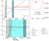 |
Fig. 1. Internal structure of the model with Z = 0.0002, M = 0.78 M⊙, Λe = 0.6, and αth = 50. Top-left and bottom-left panels are the illustrations at the ±0.5 dex point above and below the RGB-bump luminosity (Lb). The top-right panel is the zoom-in on the structure of log μ at the outer layers, which is marked by the pink band on the top-left panel. The cyan-shaded area indicates the thermohaline instability. The grey-hatched area indicates the envelope overshooting region. The grey-dotted area indicates the H-burning shell. The green lines are the decay timescale of different reactions (in 108 yrs). |
In the model after the RGB bump (bottom-left panel), the H-burning shell has already erased the chemical discontinuity left by the first dredge-up. The region of efficient nuclear shell burning (grey-dotted area), marked by the steep decrease of the 3He abundance, is much below the bottom envelope Schwarzschild border and cannot be reached even with overshooting mixing. However, in this region, the molecular weight is also sensitive to 3He destruction by 3He(3He,2p)4He and 3He(4He,γ)7Be reactions. Since, as shown in the figure, the 3He(3He, 2p)4He reaction (solid green line) is faster than the 3He(4He,γ)7Be one, an extended stratification with negative ∇μ is produced between the 3He-burning shell and the bottom of the envelope convective region. Thus, because of the thermohaline instability and envelope convection, ashes from the H-shell nuclear reactions can reach the stellar photosphere.
2.4. Effect of different efficiency values of αth
We recall that in the current investigation, we have only investigated the effects of the thermohaline mixing process in the H-rich envelopes of RGB models. To see how the efficiency of the thermohaline mixing process varies along the RGB, in Fig. 2 we compare the internal variation of Dth at six typical stages along the evolution of the calculated models. The x-axis represents the mass fraction above the H-exhausted core relative to the mass of the inter-shell between the core and the convective envelope,
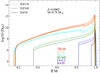 |
Fig. 2. Variation of thermohaline diffusion coefficient within the radiative region, at five typical stages along the evolution of a selected star, 0.78 M⊙. The x-axis is the relative mass in Eq. (4). Models with different thermohaline efficiency parameters, αth = 50, 100, 150, (referred to as ‘TEP’) are displayed with different line styles, while colours indicate the five stages: at the base of the RGB (BASE), 0.5 dex below the bump’s luminosity (Lb-0.5), at the bump’s luminosity (BUMP), 0.5 dex above the bump (Lb+0.5), 1 dex above the bump (Lb+1), and at the tip of the RGB (TRGB). |
where Mr is the mass coordinate and Menv, Mc are the values at the base of the convective envelope, and where the hydrogen core mass fraction is Xc < 10−7, respectively. Namely, δM = 0 marks the border of the inner core while δM = 1 marks the base of the envelope.
One can see that, as the star ascends the RGB, the thermohaline mixing process becomes more efficient, with Dth increasing by order of magnitudes, with αth modulating its efficiency. The growth of Dth is due to the rapid increase of thermal diffusivity, K, due to the decrease in mass density during the evolution of red giant stars. For example, in models with the same αth = 50 (see Fig. 1), logDth changes from 0.66 dex (Lb−0.5 model) to 2.22 dex (Lb+0.5 model) at the Schwarzschild border, while the thermal diffusion coefficient changes from 9.034 dex to 11.86 dex correspondingly. This can be understood by the inverse relation of thermal diffusivity with density. In other words, the expansion during the giant phase leads to a significant decrease in the density and hence to a rise in thermal diffusivity, and so in Dth. Another interesting point is that the instability region grows in size (in terms of relative mass), from the base of the envelope to the H-burning shell region, along the evolution of the stars. Finally, the strength of thermohaline directly depends on its efficiency parameter, that is, the larger αth, the higher Dth. As a consequence, the additional mixing directly changes the distribution of chemical elements and, eventually, the further evolution of the stars during the RGB.
Concerning the differences in the Hertzsprung–Russell diagram (HRD), in Table 1 we compare the average luminosity of the bump between the maximum and minimum values (log Lavg/L⊙), the size of the bump in terms of log L/L⊙ (meaning, the difference between the minimum and maximum luminosity of the bump), and the luminosity and age at the tip of the RGB phase. A larger value of αth leads to a slightly more luminous RGB bump and to a slightly larger difference between the minimum and maximum luminosity of the bump, which, in turn, leads to a slightly lower RGB tip luminosity and a younger RGB tip age. However, it should be emphasised that the differences here are rather modest. As expected, changing Λe has a more significant impact, especially on the location of the bump. A typical value seen from our model’s prediction is about 0.024 dex difference between the Λe = 0.5 and 0.6 models. Meanwhile, estimation from observation establishes that a typical value of the magnitude dispersion of the RGB bump in the low metallicity domain is about 0.03 dex (see Nataf et al. 2013), which corresponds to ∼0.012 dex dispersion in luminosity.
Location and size of the RGB bump, together with the luminosity and age at the tip of the RGB of a given model with 0.78 M⊙, Z = 0.0002 and for four values of αth = 0 − 150, and two sets of models with Λe = 0.5 and 0.6.
2.5. Chemical abundances
Since thermohaline mixing can convey elements from the inner H-shell to the base of the outer convective envelope, its largest effect is expected to appear in the abundance evolution of those elements, particularly at the stellar surface. In Fig. 3, we show the structure of ten chemical elements from 1H to 18O in the radiative zone between the central core and the envelope of a star 0.78 M⊙, Z = 0.0002, at the same five stages of Fig. 2.
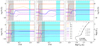 |
Fig. 3. Variation of chemical elements from 1H to 18O in five stages along the RGB phase of a selected star with initial mass 0.78 M⊙ and metallicity Z = 0.0002. The HRD of the corresponding star begins from the zero-age main sequence, with the five marked stages. Each element is indicated by the coloured lines. The cyan-shaded area displays the thermohaline instability region at each evolutionary stage (bottom-right panel), the grey-dotted area indicates the H-burning shell. All first five panels share the same scale on the x- and y-axis. |
At the base of the RGB phase, 3He accumulates as a result of the pp-chain nuclear reaction from the main sequence and reaches its peak in the shells above the central core. It is brought up to the convective envelope at first and then transported down to the region of the H-burning shell due to the 1DU later on.
In the deeper layers, the variations in 12C and 13C result from the competition between 12C(1H,γ)13N(e++νe)13C and 13C(1H,γ)14N(1H,γ)15O(e++νe)15N(1H,4He)12C via the CNO-I cycle. In deeper layers, the depletion of 17O and 18O results from the ON cycle that enriches 16O and creates its plateau. The variation of 14N and 15N is also a consequence of the competition between those nuclear processes.
Further towards the RGB bump, at which the penetration of the convective envelope has its maximum extension, 3He is already engulfed down to the H-burning shell regions. Up to this point, the inner temperature is high enough to ignite the 3He reactions and enlarge the region of thermohaline instability. During further evolution up to the tip of the RGB, the efficient thermohaline region increases in size, and mixes the inner layers above the H-burning shell with the external envelope. As a consequence, thermohaline mixing enriches the abundance of 14N while 12C and 13C and 15N are depleted. Overall, throughout the whole RGB phase, thermohaline mixing results in a depletion of the surface abundance of 3He, 7Li,12C, 13C, 15N, 18O, 19F, and 22Ne, and an increase of 14N, 17O, and 23Na, while the surface abundances of other heavier elements remain unaffected because they are not involved in nuclear reactions at this early stage of evolution.
Of particular interest is the surface abundance evolution of 3He, 7Li, 12C, and 13C during the RGB phase. The first element drives the thermohaline process, while the abundance of the other elements is commonly used to probe the internal mixing of low-mass giant stars by comparing their observed values.
Figure 4 shows the evolution of the surface abundances3 of 3He, 7Li, 12C and C-isotopic ratio4, as a function of the stellar luminosity for a star with M = 0.78M⊙, Z = 0.0002, and different assumptions of the envelope overshooting and thermohaline parameters, as indicated in the caption. The first hump of the 3He abundance at log L ∼ 1 is the result of 1DU. Corresponding with this hump, we note a strong decrease of 7Li, an increase of 12C, and a plateau in the 12C/13C abundance ratio. The following variation up to log L ∼ 1.3 is produced by the further penetration of envelope convection up to its maximum depth. After that, surface abundances remain unchanged while, in the meantime, the H-burning shell advances until it reaches the discontinuity left by the maximum penetration of envelope convection. This happens at the RGB bump at log L ∼ 2 for the adopted models. It is worth noting the barely visible variation in the RGB bump luminosity and the more conspicuous effect on A(7Li) and the 12C/13C ratio, which are produced by the different assumptions of envelope overshooting efficiency. These points will be discussed in more detail in Sect. 3.
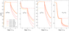 |
Fig. 4. Comparison between different models of the variation surface abundances of 3He, 7Li, 12C, and C-isotopes ratio. The models with different values of Λe = 0.5, 0.6, and αth = 0, 50, 100, 150 by using solar-scaled and [α/Fe] = 0.4 mixtures are shown according to the indicated labels. For simplicity, only the evolution during the red giant phase is shown here. |
As the H-shell moves forward to the discontinuity, which remains very near to the base of the convective envelope but without thermohaline circulation (model EOV0.5_TEP0, dotted red line), there will be no further mixing between these two regions. However, in the presence of thermohaline, the mixing continues with an efficiency that strongly depends on the thermohaline efficiency parameter (Charbonnel & Zahn 2007a; Cantiello & Langer 2010). Finally, we can see how the variation in 12C is due to mixing compared to its variation due to α-enhancement.
From the above discussion, we conclude that the envelope overshooting efficiency establishes the location of the H discontinuity in the interior structure, and thus the luminosity of the RGB bump. It also affects the surface abundance of Li at the RGB. On the other hand, the efficiency of thermohaline mixing drives the subsequent depression of A(7Li), A(12C), and of the 12C/13C ratio (see also Henkel et al. 2017; Aguilera-Gómez et al. 2023, and references therein). In the next sections, we use these two different effects to disentangle the two processes and to calibrate the thermohaline and envelope overshooting efficiency parameters.
3. Distance-independent calibration of αth and Λe from Li-abundance in NGC 6397
In order to constrain the thermohaline efficiency parameter αth in Eq. 2, we compare our model predictions with the 7Li abundance of 349 stars of the metal-poor GC NGC 6397 from Lind et al. (2009), and the 12C abundances from Briley et al. (1990). Furthermore, the relative distance between the Li-peak on the sub-giant and the location of the RGB bump implies a robust calibrator for envelope overshooting. These are discussed in detail below.
3.1. Li-abundances and thermohaline mixing
NGC 6397 is one of the most metal-poor GCs. Determination of its metallicity has been pursued in many works; for instance, Gratton et al. (2003) estimate the metallicity to be [Fe/H] = −2.03 ± 0.05, Lind et al. (2009) determine [Fe/H] = −2.10, while Korn et al. (2007) find [Fe/H] = −2.28 ± 0.04 for turn-off stars and [Fe/H] = −2.12 ± 0.03 for RGB stars, the difference being attributed to atomic diffusion. The distance modulus of NGC 6397 has also been studied in many individual works, from the colour-magnitude diagram (CMD) fitting to kinematic simulations and parallax analysis. For instance, Reid & Gizis (1998), Gratton et al. (2003), Hansen et al. (2007), Valcin et al. (2020), and Gontcharov et al. (2023) report an estimated distance of about ∼2.46 − 2.67 kpc by using CMD fitting. Also using the CMD fitting method, Correnti et al. (2018) derive a distance of 12.02 ± 0.03 mag (∼2.53 kpc). The N-body model-fitting method performed in Baumgardt et al. (2019) for 154 Galactic GCs gives a distance of 2.45 ± 0.04 kpc for NGC 6397. A trigonometric parallax analysis of the cluster by Brown et al. (2018) gives a distance of 2.39 ± 0.17 kpc, taking into account contributions from both statistical and systematic errors, and Baumgardt & Vasiliev (2021) give a mean distance of 2.482 ± 0.019 kpc. We notice that differences in the adopted distance modulus can lead to a reasonably uncertainty of ∼0.1 dex to the derived luminosity for NGC 6397. The age of this cluster is estimated to lie between 12.5–13.5 Gyr within the estimated uncertainties (see Gratton et al. 2003; Dotter et al. 2010; VandenBerg et al. 2013; Correnti et al. 2018; Tailo et al. 2020; Ahumada et al. 2021). The turn-off mass is about 0.78 M⊙ (see Korn et al. 2007).
We adopt the lithium abundance of a total of 349 stars spanning from the main-sequence (MS) turn-off point to the RGB from Lind et al. (2009) for the purpose of calibration. Recently, Wang et al. (2021) have provided a grid of synthetic spectra and abundance corrections taking into account the combined effect from 3D+NLTE, which is provided in the BREIDABLIK package5. Taking advantage of this more recent update, we re-derived the abundance of all stars in the Lind et al. sample from their reported equivalent widths and used them in this work. The comparison between data derived with 3D and 1D NLTE corrections is shown in Fig. 5 for all stars from the dwarf-MS to red giants. We find that for those stars below the RGB bump, there is an abundance shift of at most ∼ + 0.05 dex between the 3D and 1D NLTE corrections. For those stars located above the bump, the difference tends to increase up to a value of ∼ − 0.15 dex. Most importantly, the corrections in the two domains have different signs, which change the overall trend.
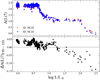 |
Fig. 5. Comparison of A(7Li) in GC NGC 6397 using 3D and 1D NLTE corrections. Top-panel: Derived abundances of all stars in the Lind et al. sample. Bottom-panel: Difference in A(7Li) between the two methods. |
Among 90 RGB stars, there are seven stars located at the luminosity above the RGB bump, which requires an extra mixing to be reproduced (see Korn et al. 2007; Henkel et al. 2017). In Fig. 6, we compare the variation of A(7Li) along the evolution of stellar models of M = 0.78M⊙ and Z = 0.0002 with the data, which is appropriate for the early post-MS evolution of NGC 6397. While it is well known that the 1DU event is responsible for the first falling branch in the low-luminosity domain around the RGB base in Fig. 6, in standard models (with no extra mixing and αth = 0, model EOV0.5_TEP0) the abundance of 7Li remains constant after the bump since there is no further mixing. However, in the presence of thermohaline mixing, 7Li diffuses downward from the envelope, which leads to the second falling branch above the RGB bump. Here, we would like to stress that it is difficult to draw firm conclusions from the four most luminous stars in the Lind et al. (2009) sample because they only have upper limits on the 7Li abundance. Therefore, we chose the three stars that are nearest to the bump as our best-fit constraint (circled in green). Indeed, the lithium abundance of these three stars is very well predicted by our model with αth = 50.
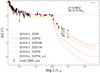 |
Fig. 6. Variation of 7Li abundance versus luminosity of giant stars. The computed track with Λe = 0.5 and solar-scaled mixture is shown in red, with four values of αth = 0, 50, 100, 150 shown by different line styles. The yellow lines show tracks with Λe = 0.6, αth = 50 using solar-scaled mixture (solid) and [α/Fe] = 0.4 mixtures (dotted). The error bar in the upper right indicates the typical 0.1 dex uncertainty in log L. |
Besides that, in Fig. 6 we show the models that are calculated with an envelope overshooting efficiency parameter of Λe = 0.5, which is the value used in PARSEC v2.0 models, and a higher value of Λe = 0.6. As can be seen, A(7Li) changes significantly when the efficiency of envelope overshooting is changed. In constrast, the variation in 7Li abundance is very similar between models computed with solar-scaled and α-enhanced mixtures. To better understand this point, Fig. 7 shows the differences in A(7Li) between models with Λe = 0.5 and models with Λe = 0.6 (top panel), and between models with solar-scaled and α-enhanced mixtures (bottom panel) for a few models with a given initial mass. In the case of the 0.78 M⊙ model, a minimum of ∼0.16 dex difference is found when varying Λe from 0.5 to 0.6 at the early phase below the bump. The discrepancy tends to be larger after the bump, with a maximum difference of about ∼0.3 dex. The absolute value of the change also depends on the initial mass, as shown in the figure. Namely, the higher the mass, the smaller the difference. On the other hand, the maximum difference between the two models of using solar-scaled and [α/Fe] = 0.4-mixtures is ∼0.04 dex, in all models, as can be seen in the bottom panel.
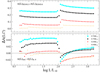 |
Fig. 7. Difference in A(7Li) between models in Fig. 6. Top-panel: Difference between track with Λe = 0.5 and Λe = 0.6, by using the solar-scaled mixtures. Bottom-panel: Difference between track using solar-scaled and α-enhanced mixtures, with the same value Λe = 0.6. |
For a more refined calibration, we computed several low-mass models, in the range of masses M = 0.64 − 0.94 M⊙, for two initial metallicity sets, Z = 0.0001, 0.0002, with the [α/Fe] = 0.4 mixture. For each metallicity set, we computed models with both values of Λe = 0.5 and 0.6 and a value of αth = 50. All models were set up with an initial lithium value of A(7Li) = 2.72. Additionally, we also computed a set with Λe = 0.6 and αth = 100, and a set with Λe = 0.05 and αth = 50 for the sake of comparison. Then, together with our newly computed models, we adopted the very-low-mass models6 (M ≤ 0.60 M⊙) from the PARSEC v1.2s dataset7 to produce the corresponding isochrones. The isochrones are produced by the recent version of the TRILEGAL code (more details of the interpolation scheme can be found in Girardi et al. 2005; Marigo et al. 2017; Bertelli et al. 1990, 2008) and converted into the photometric magnitudes by using the YBC table8 (Chen et al. 2019).
As the first step in the analysis, Fig. 8 shows the observed CMD of GC NGC 6397 in Gaia DR3 pass-bands, superimposed with our isochrones (αth = 50). We note that, for simplicity, the isochrones are limited up to the tip of the RGB phase. In Fig. 8, we adopt the distance modulus (m − M)0 = 12.05 mag from Correnti et al. (2018), and initial the metallicity Z = 0.0002 (Y = 0.249, which corresponds to [Fe/H]= − 2.088 with [α/Fe] = 0.4). Our best-fit isochrones imply an extinction of AV = 0.58 mag and an age of 12.8 Gyr, which are in good agreement with the literature (Correnti et al. 2018; Gontcharov et al. 2023, and others). Overall, our isochrones perform well, yielding a global fit from the low-MS part up to the lower red-giant branch of the cluster. Furthermore, the location of the bump selects the best-fitting model with Λe = 0.6 and [α/Fe] = 0.4-mixture. The upper branch of the RGB shows an offset from the observed data, which is a problem seen in many globular clusters (Cohen et al. 2015). The discrepancy could be due to many physical factors that are used in computing the stellar models, such the efficiency of convective energy transport (mixing-length parameter, density inversion, etc.), diffusion, mass loss, or systematic errors in the adopted bolometric corrections and metallicity (see VandenBerg et al. 2013; Correnti et al. 2018). On this note, we recall that PARSEC’s standard prescriptions for these physical processes are used in this work (see Sect. 2.2). A thorough analysis of this problem is beyond the scope of this work and will be addressed in a coming work.
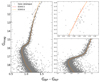 |
Fig. 8. Colour-magnitude diagram of GC NGC 6397 in Gaia DR3 pass-bands. The data is taken from the Gaia EDR3 catalogue (Vasiliev & Baumgardt 2021). The isochrones are shown with the adopted parameters (m − M)0 = 12.05 mag, [Fe/H] = −2.088, Av = 0.58 mag, and age t = 12.8 Gyr. The two panels on the right-hand side are zoomed-in on the bump and main-sequence areas. |
After obtaining constraints on the photometric properties from the CMD fit, we proceed to the comparison with the observed 7Li-abundance trend. Figure 9 shows the re-derived 3D+NLTE lithium abundances and the variation in A(7Li) from our models versus luminosity. It should be noted that the models shown in Fig. 9 are obtained from the best-fitting CMD above. We also include a model with αth = 100 in the plot for the sake of comparison. Investigating the comparison, one can see that the shape of lithium depletion after the RGB bump is the feature that verifies the constraint on the efficiency of thermohaline mixing. A reasonable uncertainty of ±0.1 dex due to the absolute value of A(7Li) from the previous phases claims the best-fitted value is αth = 50. The model with αth = 100 enhances the efficiency of thermohaline mixing too much. It is also clear that high overshoot efficiencies engulf the surface lithium too much during the early MS; on the contrary, the observed data show a well-known Spite-plateau. This point will be further discussed in the next sub-section. Despite this, the location of thermohaline’s onset (in log L) shows its best-fit to the model with Λe = 0.6.
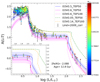 |
Fig. 9. Isochrone fitting of the observed 7Li-abundance data. The model that gives the best CMD fit in Fig. 8 is compared to the 3D+NLTE-corrected data from Lind et al. (2009). Models with (Λe = 0.6, αth = 100), (Λe = 0.14, αth = 100), and one with (Λe = 0.05, αth = 50) are also plotted here for the sake of comparison. The insert panel zooms in on the onset of thermohaline mixing. The colour bar indicates the observed masses (Masses are derived from g, Teff, and L values provided by Lind et al. 2009.). |
Furthermore, we also include in Fig. 9 the model with Λe = 0.05. By changing the efficiency, Λe, the RGB bump’s location changes significantly; for example, an ∼0.15 dex difference (in log L) can be seen between the models with Λe = 0.05 and 0.6. In the meantime, the location of the Li peak on the sub-giant branch remains almost unchanged between models (≤0.005 dex difference). This result will be revisited in detail below.
Finally, for comparison, our best-fitting thermohaline efficiency parameter is lower than the result of Henkel et al. (2017) who get Ct = 150, while our results indicate αth = 50, which corresponds to Ct = 75. We also notice that their models use an envelope overshooting value of 0.14Hp while in this work we calibrate and use a higher value, either Λe = 0.5 or 0.6. The orange line in Fig. 9 represents our model computed with their best-fit parameters (Λe = 0.14, αth = 100). However, we should emphasise that a comparison between stellar codes could be challenging due to differences in methodology and input physics; dedicated work on this matter is therefore beyond the scope of this paper and worth a separate study in the near future.
3.2. Spite plateau
The predicted amount of lithium formed in the early universe is up to three times larger than the observed abundance in halo field and globular-cluster stars (e.g. Charbonnel & Primas 2005; Bonifacio 2002; Korn et al. 2007). For instance, Spite & Spite (1982a,b) showed that old stars in a certain range of effective temperatures display a similar amount of lithium (A(Li7)≈2.2), making up the so-called Spite plateau (see also, Spite & Spite 2010). Coc et al. (2012) used the measured number of baryons per photon from the Wilkinson Microwave Anisotropy Probe satellite (Komatsu et al. 2011) to constrain the primordial value A(Li7)≈2.72 dex. Later on, Coc et al. (2014) updated their results by using the cosmological parameters determined by Planck (Planck Collaboration XVI 2014), which resulted in a slightly lower average value,  dex. The discrepancy between the measured A(Li7) and its prediction from Big Bang nucleosynthesis is known as the ‘cosmological lithium problem’.
As shown in the section above, applying a high-efficiency value of envelope overshooting during the early MS might lead to an over-depletion of lithium in the Spite-plateau area. Indeed, Christensen-Dalsgaard et al. (2011) investigated the convective envelope overshooting of the Sun by using helioseismic data. They found a mild value of Λe ≈ 0.37 reproduced the measured data very well. Later, Molaro et al. (2012) and Fu et al. (2015) proposed a new scenario to explain the 7Li depletion during the PMS. These authors suggested that a high-efficiency overshooting, mass-independent parameter, may cause a significant PMS 7Li destruction, but then, in the late PMS, a residual accretion can restore 7Li almost to the pristine value.
In this section, we take a further step in our model construction by introducing a simple scheme that purely explores the role of envelope overshooting. In particular, a milder value of the overshooting efficiency parameter is used during the evolution before it reaches the end of the MS. For the post-MS phases, a value of Λe = 0.6 is used based on the best-selected model on the CMD fitting and the onset’s location of thermohaline mixing above.
We computed several grids of models with different values of envelope-overshoot efficiency for the early evolution (from the beginning of the PMS to the end of the MS) and applied the efficiency Λe = 0.6 for the rest of the evolution. To avoid confusion, the prior value that applied to early-MS phases is noted as  . Primordial lithium, A(7Li) = 2.69, is adopted for the initial lithium abundance used in the models. For the sake of clarity regarding the trend of the observed abundances, especially in the region around the lithium peak on the sub-giant branch, we use abundance values averaged over luminosity bins (i.e. dlog L = 0.1 dex for log L ≤ 0.57, 0.01 dex for log L = 0.57 − 0.65, and 0.05 dex for the rest). Fig. 10 shows the averaged observed abundances and the predicted surface lithium abundances of models with different
  . We also apply a shift of +0.05 dex in log L to the data in order to match the peak with the isochrones. The constrained age and metallicity are adopted from the CMD fitting above. The averaged plateau clearly favours a model with a low value of envelope overshooting,
  . However, the strength of the peak before the 1DU sets in identifies a best-fitting value,
  . This result is in good agreement with the calibration of Christensen-Dalsgaard et al. (2011).
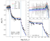 |
Fig. 10. Variation in 7Li-abundance in average values (black squares) with our models of various overshooting efficiencies at the early evolution. The applied values of |

We take one more step in relation to this aspect. As shown in Fig. 9, the colour bar shows a clear mass tendency of these stars, that is, higher mass stars have evolved to higher luminosities, while the Spite plateau shows an almost constant A(7Li). The low-mass PMS stars have deep convective zones after they leave their birthlines, and the lower the mass, the deeper the convective boundary the star will have. Meanwhile, the temperature at the base of the envelope during the first few Myrs of evolution is typically about ∼3 × 10⁶ K depending on its initial mass. Lithium, in turn, is very fragile as the nuclear reaction rate of 7Li(p, α)4He is already efficient in this range of temperatures. Therefore, the destruction of lithium during this early phase becomes very sensitive to the efficiency of overshooting, since the latter increases the temperature at the base of the mixed envelope. The variation of envelope overshooting efficiency with initial mass was already introduced in Bressan et al. (2012), and recently Addari et al. (2024) required such a dependency to reproduce the non-monotonic behaviour of the initial-final mass relation reported in Marigo et al. (2020). In this work, we apply this dependency on initial mass for  . Within the mass range from 0.64–0.86 M⊙ with step mass of 0.02 M⊙, the corresponding applied value of
  with a step of 0.05. This model is shown by the dash-dotted blue line, labelled as “growth”, in Fig. 10. It is evident that the new model reproduces the plateau, including the peak, quite well. However, we should emphasise that this new model is introduced to simply explore the impact of early-evolution variations of lithium before the onset of thermohaline mixing, while the effects of mixing processes on light elements such as lithium during the PMS and MS remains ambiguous (see Richard et al. 2005; Fu et al. 2015; Eggenberger et al. 2012; Dumont et al. 2021, and references therein).
Returning to the post-MS evolution, the averaged data display the renowned peak on the sub-giant branch (at log L/L⊙ = 0.66) observed in previous works (Korn et al. 2007; Lind et al. 2009) and understood as a short dredge-up of lithium from layers into which this element had previously settled by atomic diffusion. At the same time, the average luminosity of three stars at the RGB bump location is log L/L⊙ = 2.05. These two identifiable features are marked by the vertical lines in the figure panels. All our models demonstrate the fact that changing the overshooting efficiency does not change the location of the Li peak on the sub-giant branch. However, changing the overshooting efficiency changes the location of the RGB bump (see Fig. 9). This suggests a robust way to calibrate the value of envelope overshooting efficiency by using the relative distance between the peak feature of A(Li7) on the sub-giant branch and the location of the RGB bump, where lithium is about to be destroyed due to thermohaline mixing. This is a distance-independent method in the sense that the location of the RGB bump is measured relative to another feature of the same star cluster, which assures the robustness of this method. Indeed, the prediction of our model using the calibrated Λe = 0.6 shows the best fit to the data.
To conclude this subsection, we would like to emphasise that changing the efficiency of envelope overshooting at the early-MS phases does not change the photometry properties of the stars (log L, log Teff). Therefore, our model attempts for the early evolutionary phases do not change our conclusions above. Indeed, our model only shows sizeable effects on the variation of light elements such as lithium during this evolution. Heavier elements such as 12C and 13C instead show no or very little effect in very low-mass models.
3.3. C-abundances
Besides lithium, carbon abundance is also commonly used to probe the internal mixing of RGB stars. As mentioned in Sect. 2.5, the 12C/13C ratio is a more reliable calibrator than the 12C abundance alone. However, due to the limitations of available isotopic data for carbon in NGC 6397, we can only carry out our comparison with the 12C abundances. Fig. 11 shows the A(12C) of 25 RGB stars in NGC 6397 by Briley et al. (1990) over-plotted with the three models that we showed in Fig. 9. To derive the absolute V-band magnitude, we apply the extinction coefficient from Correnti et al. (2018), namely AV = 0.76 mag, to our isochrones in Fig. 11. As a matter of fact, the abundance data seems rather scattered, and our models with the values of thermohaline mixing efficiency αth = 50 to 100 seemingly cover the spread of the data. At this point, we recall from Sect. 2.5 (Fig. 4) that envelope overshooting does not play a significant role in the variation of carbon abundance.
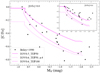 |
Fig. 11. Variation of 12C abundance with absolute V-band magnitude. The best-fit isochrones in Fig. 8 are used in this plot together with the observed data from Briley et al. (1990), with two assumptions for oxygen enhancement ([O/Fe] = 0.0 and 0.6). |
We do not know the source of this spread in the observed data. One of the factors that could explain it is the multiple populations in this cluster (Lind et al. 2011; Milone et al. 2012; MacLean et al. 2018, and references therein). To support this argument, the sub-plot in Fig. 11 shows the measured A(12C) by assuming the enhanced oxygen abundance, [O/Fe] = 0.6, reported in Briley et al. (1990). We see that our α-enhanced model fits the three stars at the lower limit of the spread very well. However, we should emphasise that a more detailed analysis would be needed to lead us to such a conclusion, and we reserve this topic for future works.
We also tested our models on the C abundance of another metal-poor GC, M92. We adopted the data from Bellman et al. (2001) and tried to fit them with our isochrones, Z = 0.0001, t = 13 Gyrs, and AV = 0.05 mag. The result gave us an offset that was about ∼0.2 dex higher than the data. We are not certain what causes this gap between the observed data and our isochrones, but we noticed that in their analysis, Bellman et al. (2001) reported different derived [C/Fe] values by using models with different input oxygen abundances. In other words, the input [O/Fe] apparently contributes to the uncertainty of the derived [C/Fe] values. For example, in many cases in their Table 4, there is a difference of about 0.1 dex between models using [O/Fe] = 0.00 and 0.3. On this note, the recent analysis of globular clusters from the Apache Point Observatory Galactic Evolution Experiment (APOGEE) survey with the BACCHUS code by Mészáros et al. (2020) shows the oxygen abundance of M92 is rather high, > 0.6 dex. Therefore, we believe the inconsistency is due to the input [O/Fe] that was assumed to derive the C abundances in Bellman et al. (2001). To conclude this section, we recognise that careful attention should be paid to the α elements in models when one uses C abundance to probe internal mixing in low-mass RGB stars. Alternatively, the 12C/13C ratio is more favourable, and we would like to explore this aspect in the near future.
4. Distance-independent calibration of Λe from seismic data of GC M4
Khan et al. (2018) have shown that a distance-independent calibration of the efficiency of envelope overshooting can be obtained by analysing the seismic properties of RGB bump stars. Here we perform a similar analysis using the available seismic data of the globular cluster M4 provided by Howell et al. (2022, hereafter H22).
Firstly, during the evolution along the RGB phase, low-mass stars make a ‘zig-zag’ path (or the RGB bump), and this is due to the interaction between the H-shell and the discontinuity. The encounter provides the H-shell with more fuel and thus leads to a temporary decrease in luminosity; shortly after, when the equilibrium is restored, the luminosity rises again. This implies that stars accumulate at this region of the CMD, which creates the RGB bump. Besides that, the location of the RGB bump is strongly correlated to the efficiency parameter of envelope overshooting. In particular, the more extended the envelope, that is, the larger Λe, the earlier the encounter occurs and hence the fainter the RGB bump is. When these properties of the RGB bump are understood, the star count distribution becomes a powerful tool to calibrate the efficiency parameter of the envelope overshooting. For example, Fu et al. (2018) used the star count distribution in a small bin of magnitude to calibrate the luminosity function of GC 47 Tuc and obtained a best-fit value of Λe = 0.5. However, by using the magnitudes for such calibration, one has to cope with the uncertainty that comes from photometric properties such as distance modulus and dust extinction.
The seismic data sample provided in H22, which claims to be the largest seismic sample in a GC to date, contains seismic data for 59 red giant stars distributed below and above the location of the RGB bump. The observed seismic quantities, namely the frequency of maximum oscillation power (νmax) and mean frequency separation of acoustic modes (Δν), can be expressed as functions of the intrinsic properties of the stars (see e.g. Ulrich 1986; Kjeldsen & Bedding 1995; Miglio et al. 2012),

where M, R, and Teff are the stellar mass, radius, and effective temperature, respectively. In Eqs. (5) and (6), the solar values are provided in H22: νmax, ⊙ = 3090 μHz, Δν⊙ = 135.1 μHz, M⊙ = 1.989 × 1033 g, R⊙ = 6.9599 × 1010 cm, and Teff, ⊙ = 5772 K.
The comparison between the observed seismic data of RGB bump stars with the corresponding one predicted by models on the basis of the above relations can thus provide another check on the robustness of the envelope overshooting model. Before proceeding with this test, we recall that the predicted seismic properties of RGB bump stars change with both the metallicity and age. To estimate these dependencies, we have calculated theoretical isochrones for the metallicity and age ranges suitable for the GC M4. M4 is a moderately metal-poor GC. In a recent analysis based on high-resolution ESO/VLT FLAMES spectroscopy of 35 RGB stars spreading from the lower branch to above the bump region, Nordlander et al. (2024) find a metallicity of [Fe/H] = −1.13 ± 0.07, in excellent agreement with previous works (e.g. Mucciarelli et al. 2011; Monaco et al. 2012; Malavolta et al. 2014; Wang et al. 2017). The cluster is confirmed to have enhanced α elements; for example, Nordlander et al. (2024) obtain [O/Fe] ∼ 0.6 dex, while Marino et al. (2008) give [α/Fe] = 0.39 ± 0.05 dex (see also Villanova & Geisler 2011; Yong et al. 2008). The age of M4 varies between 11 − 13 Gyr; for example, Tailo et al. (2022) estimate a range between 11 − 12 Gyr, while Wang et al. (2017) give 11.50 ± 0.38 Gyr, which agrees very well with McDonald & Zijlstra (2015), who find 11.81 ± 0.66 Gyr; Marín-Franch et al. (2009) claim an age of 12.65 ± 0.64 Gyr, while Hansen et al. (2002) derive an age of 12.7 ± 0.7 Gyr. We computed two initial metallicities, Z = 0.001 − 0.002, (Y = 0.250, 0.252 correspondingly), using the α-enhanced mixtures (Fu et al. 2018). The isochrones were then obtained with the TRILEGAL code for this purpose.
In Fig. 12, we show the conversion from the theoretical isochrones (log L, log Teff) to the seismic diagram (Δν, νmax), with the metallicity and age ranges suitable for the GC M4. Regarding the location of the RGB bump (insert panel), we find that changing the age from 11 to 13 Gyr affects Δν by ∼0.1 μHz and νmax by ∼0.5 μHz. Instead, by changing the metallicity from Z = 0.001 to 0.002, the variation in Δν is ∼0.5 μHz and that of νmax is ∼4.5 μHz. Thus, to obtain a sound calibration from M4 data, it is more important to determine its precise metallicity than its age.
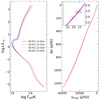 |
Fig. 12. Left: Hertzsprung–Russell diagram (HRD) of four selected isochrones, with metallicity spanning from 0.001 − 0.002 and age ranges from 11 − 13 Gyr. Right: Seismic diagram corresponding to the HRD on the left side. The inset is a zoom-in of the region of the RGB bump. The horizontal bars mark the maximum and minimum of the bump. |
To perform the seismic calibration of the RGB bump of M4, we need to identify that the H22 sample has no significant selection bias on the evolutionary stage. For this purpose, we cross-match H22 stars with the cluster member catalogue of Vasiliev & Baumgardt (2021) using Gaia Early Data Release 3 (EDR3) data. Fig. 13 shows the CMD of M4 in the Gaia EDR3/DR3 pass-bands, with data taken from Vasiliev & Baumgardt (2021). We only selected the stars that have a member probability larger than 0.95, and eliminated the horizontal branch stars for the sake of cleanliness. The 58 RGB stars from the H22 sample are indicated by the open circles. The stars were originally studied by H22 using Gaia DR2 photometry. Here, the Gaia DR3 information is obtained by cross-matching with the Gaia source_id provided by H22. We highlight the likely RGB bump stars of H22 with open blue circles and the remaining stars in H22 with open red circles (star M4RGB169 is excluded because it is not presented in the Gaia DR3 catalogue). A zoom-in on the H22 sample in the CMD around the RGB bump area is shown in the bottom-right panel of Fig. 13. In the top-right panel of Fig. 13, we show the G-magnitude function of RGB stars from Vasiliev & Baumgardt (2021, blue histogram) together with that of H22 seismic data (orange histogram). The magnitude of the RGB bump of the M4 Gaia member catalogue, Gmag ∼ 13 mag, is marked by the grey arrow. The G-magnitude function of the H22 seismic data (orange histogram) presents a peak that is consistent with the Gaia member RGB bump. This is strong evidence that the H22 sample has no significant selection bias on the evolutionary stage compared to the Gaia Vasiliev & Baumgardt (2021) sample. With this evidence, we can safely use the H22 seismic data to calibrate the RGB bump stellar models.
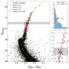 |
Fig. 13. Colour-magnitude diagram of M4 with data from the Gaia EDR3 catalogue (Vasiliev & Baumgardt 2021) with the isochrones shown in Fig. 14. The adopted parameters for the isochrones are 12.6 Gyr, Z = 0.0015, (m − M)0 = 11.35 mag, and Av = 1.3 mag. The open circles are stars from the Howell et al. (2022) sample. Top-right: Star count histogram on Gmag with a magnitude bin of 0.3 dex along the RGB. Bottom-right: Zoom-in of the RGB bump area. |
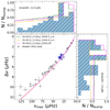 |
Fig. 14. Seismic diagram of 58 RGB stars in Howell et al. (2022). The selected isochrones with a variation of Λe = 0.05, 0.5, 0.6 are superimposed by solid lines. The distinguished excess stars in the H22 sample are circled in blue. Star count histograms on νmax and Δν are shown in the top and right panels, correspondingly, in which the blue-hatched area indicates the H22 data and the lines represent model predictions. |
We now compare the observed seismic properties of the H22 RGB stars with those predicted by assuming a different efficiency of envelope overshooting; we do this in Fig. 14. The top panel of Fig. 14 shows the histogram of star count distribution in νmax with a step of 12 μHz. The bottom-right panel shows the Δν histogram with a step of 1 μHz. The star count is normalised to its maximum value within the range, with the peak region referred to the distinguished RGB bump stars (blue circle). The theoretical luminosity function is computed by adopting an age of 12.6 Gyr (see Marín-Franch et al. 2009), and an initial metallicity that produces the measured metallicity of Nordlander et al. (2024), in the bump region. It should be mentioned that Nordlander et al. (2024) adopt Grevesse et al. (2007) solar compositions, while we adopt the compositions from Caffau et al. (2011). In other words, the rescaled metallicity due to the difference in solar reference composition is [Fe/H] = −1.2 dex. This value corresponds to Z = 0.0015 with our adopted [α/Fe] = 0.4 mixture. The solid lines in Fig. 14 show the prediction from theoretical models with this metallicity, and with different values of envelope overshooting parameter. The computed model with α-enhanced mixture and Λe = 0.6 shows the best fit to the observed star count histogram, while the model with lower values, Λe = 0.05 (adopted from PARSEC v1.2S) and Λe = 0.5, predict a frequency of the bump that is too low to reproduce the observed data. It should be emphasised that this result holds for histograms performed in both Δν and νmax. We also check this best-fit model on the CMD as shown in Fig. 13, together with the model of Λe = 0.5 for comparison. The isochrones are applied with the adopted distance modulus (m − M)0 = 11.35 mag (see Baumgardt & Vasiliev 2021), and extinction coefficient Av = 1.3 mag (see Hendricks et al. 2012, and references therein).
Furthermore, the multi-populations feature in the GC M4 has been studied in many works that have shown that the He content plays a key role. We know that one population is formed with He enrichment, while the other population has a normal He content that is compatible with the primordial value and located at the redder part of the cluster (e.g. Villanova et al. 2012; Valcarce et al. 2014; D’Antona et al. 2022; Costa et al. 2024). However, a detailed analysis of the multiple populations in M4 is beyond the scope of this paper. However, it is worth mentioning that we compute our models by following the standard enrichment law for He content (Bressan et al. 2012). As a result, our isochrones give a good fit to the observed CMD, from the lower part of the MS up to the tip of the RGB. As an aside, we would like to mention that He content could be the cause of the mismatch on the lower RGB in Fig. 14. However, this does not affect our conclusions since we focus on the upper part of the diagram where the RGB bump is located. A detailed analysis of this aspect is reserved for a coming work.
Finally, to conclude this section, we would like to stress that the model with Λe = 0.6 shows the best fit to the seismic star count distribution of GC M4. This result supports our finding in Sect. 3. In other words, we have performed two independent calibrations, both distance- and reddening-independent, for the envelope overshooting parameter, and obtained good agreement with observations for Λe = 0.6. Although the two clusters we use for our calibrations have different metallicities, they are both in the low-metallicity domain [Fe/H] = [−2.09,−1.21], that is, ∼0.9 dex apart. We note that the brightness of the RGB bump of several GCs across a certain range of metallicity is well reproduced with a single envelope overshooting parameter as stated in Fu et al. (2018) (see their Fig. 14, [Fe/H] ∼ [−1.3, −0.75]; see also Khan et al. 2018). Our results point in the same direction, but for a lower-metallicity domain.
5. Summary and conclusions
In this paper, we first present the implementation of thermohaline mixing in the PARSEC code, and second the interplay between thermohaline mixing and envelope overshooting in low-mass stars. We explore the effects of these mixing processes on the surface abundance of lithium and carbon in Sect. 2.5, together with variations in the adopted chemical mixtures. The efficiency parameters of these processes control the amount of abundances measurable at the stellar surface. Using 2012AJ....144...25Hobserved data on two well-studied globular clusters (NGC 6397 and M4), we performed calibrations on the efficiency of the thermohaline mixing parameter, αth, and on the envelope overshooting parameter, Λe, in Sects. 3 and 4.
For theoretical models, we used the most recent version of the PARSEC code (Costa et al. 2019b; Nguyen et al. 2022) with the implemented thermohaline mixing. Four sets of initial metallicity, Z = 0.0001, 0.0002, 0.001, 0.002, were computed, with variation in the efficiency parameters. Each metallicity set contains 14 stellar tracks with masses spanning from 0.64 − 0.94 M⊙. The corresponding isochrones were then produced using the TRILEGAL code with the adoption of very-low-mass models from the previous PARSEC V1.2S. Then, they were complemented with the YBC bolometric correction tables for the benefit of our calibrations.
In this work, thermohaline mixing is treated as a diffusive process, and we follow the standard scheme of Charbonnel & Zahn (2007a) and Cantiello & Langer (2010) to model it. We carefully study the impact of thermohaline mixing on evolution and changes in chemical abundances.
We performed calibration on the thermohaline mixing efficiency parameter based on the observed 7Li abundances of stars in GC NGC 6397 from Lind et al. (2009). To work with the latest 3D+NLTE abundances, we re-derived the inferred abundances from the lines’ equivalent widths by using the BREIDABLIK package (Wang et al. 2021). A relatively small value of αth = 50 was obtained to reproduce the lithium abundance of three stars above the RGB bump. Moreover, our attempted models with smaller envelope overshooting efficiencies for the PMS and MS phases, and Λe = 0.6 for the post-MS, together with the thermohaline efficiency parameter αth = 50, gives the best fit to the 3D+NLTE lithium abundances of GC NGC 6397, from the Spite-plateau to the RGB stars. Furthermore, the luminosity difference between the Li-peak on the sub-giant and the onset of thermohaline mixing at the RGB bump implies a robust calibration with Λe = 0.6.
An independent and alternative approach to calibrate the efficiency of envelope overshooting was done by using the seismology data of GC M4. In this analysis, we focus on the star count distribution in both the frequency of maximum oscillation power, νmax, and the mean frequency separation of acoustic modes, Δν, to draw our conclusion on the best-fitting value for Λe. As a result, we find that Λe = 0.6 is required to reproduce the accumulation of stars at the RGB bump of M4. This result agrees with the former one, and thus strengthens our conclusion.
Finally, we would like to stress that even though rotation has been implemented in the PARSEC code (Costa et al. 2019b; Nguyen et al. 2022), we do not consider it in the present work. We focus on the effect of convective envelope overshooting and thermohaline mixing along the post-MS phases. The impact of rotation on thermohaline mixing has already been investigated in the literature (e.g. Charbonnel & Lagarde 2010; Lagarde et al. 2011). Moreover, Maeder et al. (2013) pointed out that the horizontal turbulence in rotating stars can inhibit thermohaline mixing, which led to an even more complex scenario. A project combining all these effects is deferred to the future.
The re-derived 3D+NLTE lithium abundance of NGC 6397, together with the stellar tracks of our best-fit models that are presented in this paper, can be archived at the dedicated ZENODO dataset9. The isochrones with different photometric pass-bands can be provided upon request.
Acknowledgments
The authors are in deepest sorrow with the passing of Prof. Paola Marigo on October 20, 2024. We wish to express our gratitude for her dedications and guidance over the years. We thank the anonymous referee for the insightful comments and suggestions to improve the paper. CTN also thanks Madeline Howell for providing useful seismic data information. This project has received funding from the European Union’s Horizon 2020 research and innovation programme under grant agreement No 101008324 (ChETEC-INFRA). AB acknowledges the Italian Ministerial grant PRIN2022, “Radiative opacities for astrophysical applications”, no. 2022NEXMP8. GC acknowledges support from the Agence Nationale de la Recherche grant POPSYCLE number ANR-19-CE31-0022. X.F. acknowledges the support of the National Natural Science Foundation of China (NSFC) No. 12203100 and the China Manned Space Project with NO.CMS-CSST-2021-A08. AJK acknowledges support by the Swedish National Space Agency (SNSA)
References
- Addari, F., Marigo, P., Bressan, A., et al. 2024, ApJ, 964, 51 [NASA ADS] [CrossRef] [Google Scholar]
- Aguilera-Gómez, C., Monaco, L., Mucciarelli, A., et al. 2022, A&A, 657, A33 [NASA ADS] [CrossRef] [EDP Sciences] [Google Scholar]
- Aguilera-Gómez, C., Jones, M. I., & Chanamé, J. 2023, A&A, 670, A73 [NASA ADS] [CrossRef] [EDP Sciences] [Google Scholar]
- Ahumada, J. A., Arellano Ferro, A., Bustos Fierro, I. H., et al. 2021, New Astron., 88, 101607 [Google Scholar]
- Alongi, M., Bertelli, G., Bressan, A., & Chiosi, C. 1991, A&A, 244, 95 [NASA ADS] [Google Scholar]
- Baumgardt, H., & Vasiliev, E. 2021, MNRAS, 505, 5957 [NASA ADS] [CrossRef] [Google Scholar]
- Baumgardt, H., Hilker, M., Sollima, A., & Bellini, A. 2019, MNRAS, 482, 5138 [Google Scholar]
- Beers, T. C., & Christlieb, N. 2005, ARA&A, 43, 531 [NASA ADS] [CrossRef] [Google Scholar]
- Bellman, S., Briley, M. M., Smith, G. H., & Claver, C. F. 2001, PASP, 113, 326 [Google Scholar]
- Bertelli, G., Betto, R., Bressan, A., et al. 1990, A&AS, 85, 845 [NASA ADS] [Google Scholar]
- Bertelli, G., Girardi, L., Marigo, P., & Nasi, E. 2008, A&A, 484, 815 [NASA ADS] [CrossRef] [EDP Sciences] [Google Scholar]
- Bonifacio, P. 2002, A&A, 395, 515 [NASA ADS] [CrossRef] [EDP Sciences] [Google Scholar]
- Bressan, A. G., Chiosi, C., & Bertelli, G. 1981, A&A, 102, 25 [Google Scholar]
- Bressan, A., Marigo, P., Girardi, L., et al. 2012, MNRAS, 427, 127 [NASA ADS] [CrossRef] [Google Scholar]
- Briley, M. M., Bell, R. A., Hoban, S., & Dickens, R. J. 1990, ApJ, 359, 307 [Google Scholar]
- Brown, T. M., Casertano, S., Strader, J., et al. 2018, ApJ, 856, L6 [Google Scholar]
- Caffau, E., Ludwig, H. G., Steffen, M., Freytag, B., & Bonifacio, P. 2011, Sol. Phys., 268, 255 [Google Scholar]
- Cantiello, M., & Langer, N. 2010, A&A, 521, A9 [NASA ADS] [CrossRef] [EDP Sciences] [Google Scholar]
- Charbonnel, C., & Lagarde, N. 2010, A&A, 522, A10 [CrossRef] [EDP Sciences] [Google Scholar]
- Charbonnel, C., & Primas, F. 2005, A&A, 442, 961 [NASA ADS] [CrossRef] [EDP Sciences] [Google Scholar]
- Charbonnel, C., & Zahn, J. P. 2007a, A&A, 467, L15 [NASA ADS] [CrossRef] [EDP Sciences] [Google Scholar]
- Charbonnel, C., & Zahn, J. P. 2007b, A&A, 476, L29 [NASA ADS] [CrossRef] [EDP Sciences] [Google Scholar]
- Charbonnel, C., Brown, J. A., & Wallerstein, G. 1998, A&A, 332, 204 [NASA ADS] [Google Scholar]
- Chen, Y., Girardi, L., Bressan, A., et al. 2014, MNRAS, 444, 2525 [Google Scholar]
- Chen, Y., Girardi, L., Fu, X., et al. 2019, A&A, 632, A105 [EDP Sciences] [Google Scholar]
- Christensen-Dalsgaard, J., Monteiro, M. J. P. F. G., Rempel, M., & Thompson, M. J. 2011, MNRAS, 414, 1158 [CrossRef] [Google Scholar]
- Coc, A., Goriely, S., Xu, Y., Saimpert, M., & Vangioni, E. 2012, ApJ, 744, 158 [NASA ADS] [CrossRef] [Google Scholar]
- Coc, A., Uzan, J.-P., & Vangioni, E. 2014, JCAP, 2014, 050 [Google Scholar]
- Cohen, R. E., Hempel, M., Mauro, F., et al. 2015, AJ, 150, 176 [NASA ADS] [CrossRef] [Google Scholar]
- Correnti, M., Gennaro, M., Kalirai, J. S., Cohen, R. E., & Brown, T. M. 2018, ApJ, 864, 147 [NASA ADS] [CrossRef] [Google Scholar]
- Costa, G., Girardi, L., Bressan, A., et al. 2019a, A&A, 631, A128 [NASA ADS] [CrossRef] [EDP Sciences] [Google Scholar]
- Costa, G., Girardi, L., Bressan, A., et al. 2019b, MNRAS, 485, 4641 [NASA ADS] [CrossRef] [Google Scholar]
- Costa, G., Bressan, A., Mapelli, M., et al. 2021, MNRAS, 501, 4514 [NASA ADS] [CrossRef] [Google Scholar]
- Costa, G., Dumont, T., Lançon, A., et al. 2024, A&A, 690, A22 [NASA ADS] [CrossRef] [EDP Sciences] [Google Scholar]
- Costa, G., Shepherd, K. G., Bressan, A., et al. 2025, A&A, 694, A193 [NASA ADS] [CrossRef] [EDP Sciences] [Google Scholar]
- D’Antona, F., Milone, A. P., Johnson, C. I., et al. 2022, ApJ, 925, 192 [CrossRef] [Google Scholar]
- Dotter, A., Sarajedini, A., Anderson, J., et al. 2010, ApJ, 708, 698 [Google Scholar]
- Dumont, T., Palacios, A., Charbonnel, C., et al. 2021, A&A, 646, A48 [EDP Sciences] [Google Scholar]
- Eggenberger, P., Haemmerlé, L., Meynet, G., & Maeder, A. 2012, A&A, 539, A70 [NASA ADS] [CrossRef] [EDP Sciences] [Google Scholar]
- Eggleton, P. P., Dearborn, D. S. P., & Lattanzio, J. C. 2006, Science, 314, 1580 [Google Scholar]
- Frebel, A., & Norris, J. E. 2015, ARA&A, 53, 631 [NASA ADS] [CrossRef] [Google Scholar]
- Fu, X., Bressan, A., Molaro, P., & Marigo, P. 2015, MNRAS, 452, 3256 [CrossRef] [Google Scholar]
- Fu, X., Bressan, A., Marigo, P., et al. 2018, MNRAS, 476, 496 [NASA ADS] [CrossRef] [Google Scholar]
- Girardi, L., Groenewegen, M. A. T., Hatziminaoglou, E., & da Costa, L. 2005, A&A, 436, 895 [NASA ADS] [CrossRef] [EDP Sciences] [Google Scholar]
- Gontcharov, G. A., Bonatto, C. J., Ryutina, O. S., et al. 2023, MNRAS, 526, 5628 [NASA ADS] [CrossRef] [Google Scholar]
- Gratton, R. G., Sneden, C., Carretta, E., & Bragaglia, A. 2000, A&A, 354, 169 [NASA ADS] [Google Scholar]
- Gratton, R. G., Bragaglia, A., Carretta, E., et al. 2003, A&A, 408, 529 [NASA ADS] [CrossRef] [EDP Sciences] [Google Scholar]
- Grevesse, N., Asplund, M., & Sauval, A. J. 2007, Space Sci. Rev., 130, 105 [Google Scholar]
- Hansen, B. M. S., Brewer, J., Fahlman, G. G., et al. 2002, ApJ, 574, L155 [NASA ADS] [CrossRef] [Google Scholar]
- Hansen, B. M. S., Anderson, J., Brewer, J., et al. 2007, ApJ, 671, 380 [Google Scholar]
- Hendricks, B., Stetson, P. B., VandenBerg, D. A., & Dall’Ora, M. 2012, AJ, 144, 25 [NASA ADS] [CrossRef] [Google Scholar]
- Henkel, K., Karakas, A. I., & Lattanzio, J. C. 2017, MNRAS, 469, 4600 [Google Scholar]
- Henkel, K., Karakas, A. I., Casey, A. R., Church, R. P., & Lattanzio, J. C. 2018, ApJ, 863, L5 [NASA ADS] [CrossRef] [Google Scholar]
- Howell, M., Campbell, S. W., Stello, D., & De Silva, G. M. 2022, MNRAS, 515, 3184 [NASA ADS] [CrossRef] [Google Scholar]
- Khan, S., Hall, O. J., Miglio, A., et al. 2018, ApJ, 859, 156 [NASA ADS] [CrossRef] [Google Scholar]
- Kippenhahn, R., Ruschenplatt, G., & Thomas, H. C. 1980, A&A, 91, 175 [Google Scholar]
- Kjeldsen, H., & Bedding, T. R. 1995, A&A, 293, 87 [NASA ADS] [Google Scholar]
- Komatsu, E., Smith, K. M., Dunkley, J., et al. 2011, ApJS, 192, 18 [Google Scholar]
- Korn, A. J., Grundahl, F., Richard, O., et al. 2007, ApJ, 671, 402 [NASA ADS] [CrossRef] [Google Scholar]
- Lagarde, N., Charbonnel, C., Decressin, T., & Hagelberg, J. 2011, A&A, 536, A28 [NASA ADS] [CrossRef] [EDP Sciences] [Google Scholar]
- Lind, K., Primas, F., Charbonnel, C., Grundahl, F., & Asplund, M. 2009, A&A, 503, 545 [NASA ADS] [CrossRef] [EDP Sciences] [Google Scholar]
- Lind, K., Charbonnel, C., Decressin, T., et al. 2011, A&A, 527, A148 [NASA ADS] [CrossRef] [EDP Sciences] [Google Scholar]
- MacLean, B. T., Campbell, S. W., De Silva, G. M., et al. 2018, MNRAS, 475, 257 [NASA ADS] [CrossRef] [Google Scholar]
- Maeder, A., Meynet, G., Lagarde, N., & Charbonnel, C. 2013, A&A, 553, A1 [NASA ADS] [CrossRef] [EDP Sciences] [Google Scholar]
- Malavolta, L., Sneden, C., Piotto, G., et al. 2014, AJ, 147, 25 [Google Scholar]
- Marigo, P., Girardi, L., Bressan, A., et al. 2017, ApJ, 835, 77 [Google Scholar]
- Marigo, P., Cummings, J. D., Curtis, J. L., et al. 2020, Nat. Astron., 4, 1102 [NASA ADS] [CrossRef] [Google Scholar]
- Marín-Franch, A., Aparicio, A., Piotto, G., et al. 2009, ApJ, 694, 1498 [Google Scholar]
- Marino, A. F., Villanova, S., Piotto, G., et al. 2008, A&A, 490, 625 [NASA ADS] [CrossRef] [EDP Sciences] [Google Scholar]
- McDonald, I., & Zijlstra, A. A. 2015, MNRAS, 448, 502 [Google Scholar]
- Mészáros, S., Masseron, T., García-Hernández, D. A., et al. 2020, MNRAS, 492, 1641 [Google Scholar]
- Miglio, A., Brogaard, K., Stello, D., et al. 2012, MNRAS, 419, 2077 [Google Scholar]
- Milone, A. P., Marino, A. F., Piotto, G., et al. 2012, ApJ, 745, 27 [Google Scholar]
- Molaro, P., Bressan, A., Barbieri, M., Marigo, P., & Zaggia, S. 2012, Mem. Soc. Astron. It. Suppl., 22, 233 [Google Scholar]
- Monaco, L., Villanova, S., Bonifacio, P., et al. 2012, A&A, 539, A157 [NASA ADS] [CrossRef] [EDP Sciences] [Google Scholar]
- Mucciarelli, A., Salaris, M., Lovisi, L., et al. 2011, MNRAS, 412, 81 [NASA ADS] [CrossRef] [Google Scholar]
- Nataf, D. M., Gould, A. P., Pinsonneault, M. H., & Udalski, A. 2013, ApJ, 766, 77 [NASA ADS] [CrossRef] [Google Scholar]
- Nguyen, C. T., Costa, G., Girardi, L., et al. 2022, A&A, 665, A126 [NASA ADS] [CrossRef] [EDP Sciences] [Google Scholar]
- Nordlander, T., Gruyters, P., Richard, O., & Korn, A. J. 2024, MNRAS, 527, 12120 [Google Scholar]
- Placco, V. M., Frebel, A., Beers, T. C., & Stancliffe, R. J. 2014, ApJ, 797, 21 [Google Scholar]
- Planck Collaboration XVI. 2014, A&A, 571, A16 [NASA ADS] [CrossRef] [EDP Sciences] [Google Scholar]
- Reid, I. N., & Gizis, J. E. 1998, AJ, 116, 2929 [Google Scholar]
- Richard, O., Michaud, G., & Richer, J. 2005, ApJ, 619, 538 [Google Scholar]
- Smith, G. H., & Tout, C. A. 1992, MNRAS, 256, 449 [Google Scholar]
- Spite, F., & Spite, M. 1982a, A&A, 115, 357 [NASA ADS] [Google Scholar]
- Spite, M., & Spite, F. 1982b, Nature, 297, 483 [NASA ADS] [CrossRef] [Google Scholar]
- Spite, M., & Spite, F. 2010, in Light Elements in the Universe, eds. C. Charbonnel, M. Tosi, F. Primas, & C. Chiappini, 268, 201 [NASA ADS] [Google Scholar]
- Stancliffe, R. J. 2009, MNRAS, 394, 1051 [Google Scholar]
- Stancliffe, R. J., Church, R. P., Angelou, G. C., & Lattanzio, J. C. 2009, MNRAS, 396, 2313 [Google Scholar]
- Tailo, M., Milone, A. P., Lagioia, E. P., et al. 2020, MNRAS, 498, 5745 [CrossRef] [Google Scholar]
- Tailo, M., Corsaro, E., Miglio, A., et al. 2022, A&A, 662, L7 [NASA ADS] [CrossRef] [EDP Sciences] [Google Scholar]
- Ulrich, R. K. 1972, ApJ, 172, 165 [NASA ADS] [CrossRef] [Google Scholar]
- Ulrich, R. K. 1986, ApJ, 306, L37 [Google Scholar]
- Valcarce, A. A. R., Catelan, M., Alonso-García, J., Cortés, C., & De Medeiros, J. R. 2014, ApJ, 782, 85 [NASA ADS] [CrossRef] [Google Scholar]
- Valcin, D., Bernal, J. L., Jimenez, R., Verde, L., & Wandelt, B. D. 2020, JCAP, 2020, 002 [Google Scholar]
- VandenBerg, D. A., Brogaard, K., Leaman, R., & Casagrande, L. 2013, ApJ, 775, 134 [Google Scholar]
- Vasiliev, E., & Baumgardt, H. 2021, MNRAS, 505, 5978 [NASA ADS] [CrossRef] [Google Scholar]
- Viallet, M., Meakin, C., Prat, V., & Arnett, D. 2015, A&A, 580, A61 [NASA ADS] [CrossRef] [EDP Sciences] [Google Scholar]
- Villanova, S., & Geisler, D. 2011, A&A, 535, A31 [NASA ADS] [CrossRef] [EDP Sciences] [Google Scholar]
- Villanova, S., Geisler, D., Piotto, G., & Gratton, R. G. 2012, ApJ, 748, 62 [NASA ADS] [CrossRef] [Google Scholar]
- Wang, Y., Primas, F., Charbonnel, C., et al. 2017, A&A, 607, A135 [NASA ADS] [CrossRef] [EDP Sciences] [Google Scholar]
- Wang, E. X., Nordlander, T., Asplund, M., et al. 2021, MNRAS, 500, 2159 [Google Scholar]
- Yong, D., Lambert, D. L., Paulson, D. B., & Carney, B. W. 2008, ApJ, 673, 854 [NASA ADS] [CrossRef] [Google Scholar]
All Tables
Location and size of the RGB bump, together with the luminosity and age at the tip of the RGB of a given model with 0.78 M⊙, Z = 0.0002 and for four values of αth = 0 − 150, and two sets of models with Λe = 0.5 and 0.6.
All Figures
|
Fig. 1. Internal structure of the model with Z = 0.0002, M = 0.78 M⊙, Λe = 0.6, and αth = 50. Top-left and bottom-left panels are the illustrations at the ±0.5 dex point above and below the RGB-bump luminosity (Lb). The top-right panel is the zoom-in on the structure of log μ at the outer layers, which is marked by the pink band on the top-left panel. The cyan-shaded area indicates the thermohaline instability. The grey-hatched area indicates the envelope overshooting region. The grey-dotted area indicates the H-burning shell. The green lines are the decay timescale of different reactions (in 108 yrs). |
| In the text | |
|
Fig. 2. Variation of thermohaline diffusion coefficient within the radiative region, at five typical stages along the evolution of a selected star, 0.78 M⊙. The x-axis is the relative mass in Eq. (4). Models with different thermohaline efficiency parameters, αth = 50, 100, 150, (referred to as ‘TEP’) are displayed with different line styles, while colours indicate the five stages: at the base of the RGB (BASE), 0.5 dex below the bump’s luminosity (Lb-0.5), at the bump’s luminosity (BUMP), 0.5 dex above the bump (Lb+0.5), 1 dex above the bump (Lb+1), and at the tip of the RGB (TRGB). |
| In the text | |
|
Fig. 3. Variation of chemical elements from 1H to 18O in five stages along the RGB phase of a selected star with initial mass 0.78 M⊙ and metallicity Z = 0.0002. The HRD of the corresponding star begins from the zero-age main sequence, with the five marked stages. Each element is indicated by the coloured lines. The cyan-shaded area displays the thermohaline instability region at each evolutionary stage (bottom-right panel), the grey-dotted area indicates the H-burning shell. All first five panels share the same scale on the x- and y-axis. |
| In the text | |
|
Fig. 4. Comparison between different models of the variation surface abundances of 3He, 7Li, 12C, and C-isotopes ratio. The models with different values of Λe = 0.5, 0.6, and αth = 0, 50, 100, 150 by using solar-scaled and [α/Fe] = 0.4 mixtures are shown according to the indicated labels. For simplicity, only the evolution during the red giant phase is shown here. |
| In the text | |
|
Fig. 5. Comparison of A(7Li) in GC NGC 6397 using 3D and 1D NLTE corrections. Top-panel: Derived abundances of all stars in the Lind et al. sample. Bottom-panel: Difference in A(7Li) between the two methods. |
| In the text | |
|
Fig. 6. Variation of 7Li abundance versus luminosity of giant stars. The computed track with Λe = 0.5 and solar-scaled mixture is shown in red, with four values of αth = 0, 50, 100, 150 shown by different line styles. The yellow lines show tracks with Λe = 0.6, αth = 50 using solar-scaled mixture (solid) and [α/Fe] = 0.4 mixtures (dotted). The error bar in the upper right indicates the typical 0.1 dex uncertainty in log L. |
| In the text | |
|
Fig. 7. Difference in A(7Li) between models in Fig. 6. Top-panel: Difference between track with Λe = 0.5 and Λe = 0.6, by using the solar-scaled mixtures. Bottom-panel: Difference between track using solar-scaled and α-enhanced mixtures, with the same value Λe = 0.6. |
| In the text | |
|
Fig. 8. Colour-magnitude diagram of GC NGC 6397 in Gaia DR3 pass-bands. The data is taken from the Gaia EDR3 catalogue (Vasiliev & Baumgardt 2021). The isochrones are shown with the adopted parameters (m − M)0 = 12.05 mag, [Fe/H] = −2.088, Av = 0.58 mag, and age t = 12.8 Gyr. The two panels on the right-hand side are zoomed-in on the bump and main-sequence areas. |
| In the text | |
|
Fig. 9. Isochrone fitting of the observed 7Li-abundance data. The model that gives the best CMD fit in Fig. 8 is compared to the 3D+NLTE-corrected data from Lind et al. (2009). Models with (Λe = 0.6, αth = 100), (Λe = 0.14, αth = 100), and one with (Λe = 0.05, αth = 50) are also plotted here for the sake of comparison. The insert panel zooms in on the onset of thermohaline mixing. The colour bar indicates the observed masses (Masses are derived from g, Teff, and L values provided by Lind et al. 2009.). |
| In the text | |
|
Fig. 10. Variation in 7Li-abundance in average values (black squares) with our models of various overshooting efficiencies at the early evolution. The applied values of |
| In the text | |
|
Fig. 11. Variation of 12C abundance with absolute V-band magnitude. The best-fit isochrones in Fig. 8 are used in this plot together with the observed data from Briley et al. (1990), with two assumptions for oxygen enhancement ([O/Fe] = 0.0 and 0.6). |
| In the text | |
|
Fig. 12. Left: Hertzsprung–Russell diagram (HRD) of four selected isochrones, with metallicity spanning from 0.001 − 0.002 and age ranges from 11 − 13 Gyr. Right: Seismic diagram corresponding to the HRD on the left side. The inset is a zoom-in of the region of the RGB bump. The horizontal bars mark the maximum and minimum of the bump. |
| In the text | |
|
Fig. 13. Colour-magnitude diagram of M4 with data from the Gaia EDR3 catalogue (Vasiliev & Baumgardt 2021) with the isochrones shown in Fig. 14. The adopted parameters for the isochrones are 12.6 Gyr, Z = 0.0015, (m − M)0 = 11.35 mag, and Av = 1.3 mag. The open circles are stars from the Howell et al. (2022) sample. Top-right: Star count histogram on Gmag with a magnitude bin of 0.3 dex along the RGB. Bottom-right: Zoom-in of the RGB bump area. |
| In the text | |
|
Fig. 14. Seismic diagram of 58 RGB stars in Howell et al. (2022). The selected isochrones with a variation of Λe = 0.05, 0.5, 0.6 are superimposed by solid lines. The distinguished excess stars in the H22 sample are circled in blue. Star count histograms on νmax and Δν are shown in the top and right panels, correspondingly, in which the blue-hatched area indicates the H22 data and the lines represent model predictions. |
| In the text | |
Current usage metrics show cumulative count of Article Views (full-text article views including HTML views, PDF and ePub downloads, according to the available data) and Abstracts Views on Vision4Press platform.
Data correspond to usage on the plateform after 2015. The current usage metrics is available 48-96 hours after online publication and is updated daily on week days.
Initial download of the metrics may take a while.