| Issue |
A&A
Volume 668, December 2022
|
|
|---|---|---|
| Article Number | A126 | |
| Number of page(s) | 8 | |
| Section | Stellar structure and evolution | |
| DOI | https://doi.org/10.1051/0004-6361/202243871 | |
| Published online | 13 December 2022 | |
Li-rich and super Li-rich giants produced by element diffusion⋆
1
School of Physical Science and Technology, Xinjiang University, Urumqi 830046, PR China
e-mail: This email address is being protected from spambots. You need JavaScript enabled to view it.
2
Center for Theoretical Physics, Xinjiang University, Urumqi 830046, PR China
3
College of Mechanical and Electronic Engineering, Tarim University, Alar 843300, PR China
4
CAS Key Laboratory of Optical Astronomy, National Astronomical Observatories, Chinese Academy of Sciences, Beijing 100101, PR China
5
School of Astronomy and Space Science, University of Chinese Academy of Sciences, Beijing 100101, PR China
Received:
26
April
2022
Accepted:
17
October
2022
Abstract
Context. About 0.2−2% of giant stars are Li rich, that is to say their lithium abundance (A(Li)) is higher than 1.5 dex. Nearly 6% of these Li-rich giant stars are super Li rich, with an A(Li) exceeding 3.2 dex. Meanwhile, the formation mechanism of these Li-rich and super Li-rich giants is still under debate.
Aims. Considering the compact He core of red giants, attention is paid to the effect of element diffusion on A(Li). In particular, when the He-core flash occurs, element diffusion makes the thermohaline mixing zone extend inward and connect to the inner convection region of stars. Then, a large amount of 7Be produced by the He flash can be transferred to the stellar surface, finally turning into 7Li. Thus, the goal of this work is to propose the mechanism of A(Li) enrichment and achieve consistency between the theoretical and observation data.
Methods. Using the Modules for Experiments in Stellar Astrophysics (MESA) stellar evolution code, we simulated the evolution of low-mass stars, considering the effects of element diffusion on the Li abundances. The timescale ratio of Li-rich giants to normal giants was estimated using the population synthesis method. Then we obtained the theoretical value of A(Li) and made a comparison with observations.
Results. Considering the influence of element diffusion in the model results in the increase of the lithium abundance up to about 1.8 dex, which can reveal Li-rich giants. Simultaneously, introducing high constant diffusive mixing coefficients (Dmix) with the values from 1011 to 1015 cm2 s−1 in the model allows the A(Li) to increase from 2.4 to 4.5 dex, which can explain most of the Li-rich and super Li-rich giant stars. The population synthesis method reveals that the amount of Li-rich giants is about 0.2−2% of all giants, which is consistent with observation estimated levels.
Conclusions. In our models the element diffusion, mainly triggered by the gravity field, changes the mean molecular weight at the junction zone between the stellar envelope and the He core, which makes the thermohaline mixing region expand to the inner convection region of stars. A transport channel, efficiently transporting 7Be in the hydrogen-burning region of the star to the convective envelope where 7Be decays into 7Li, is formed. Combining high constant diffusive mixing coefficients, the transport channel can explain the origin of Li-rich and super Li-rich giants, even the most super Li-rich giants.
Key words: stars: abundances / stars: evolution / stars: low-mass / diffusion / standards / gravitation
Full version of Table 1 is only available at the CDS via anonymous ftp to https://cdsarc.cds.unistra.fr (130.79.128.5) or via https://cdsarc.cds.unistra.fr/viz-bin/cat/J/A+A/668/A126
© The Authors 2022
 Open Access article, published by EDP Sciences, under the terms of the Creative Commons Attribution License (https://creativecommons.org/licenses/by/4.0), which permits unrestricted use, distribution, and reproduction in any medium, provided the original work is properly cited.
This article is published in open access under the Subscribe-to-Open model. This email address is being protected from spambots. You need JavaScript enabled to view it. to support open access publication.
1. Introduction
Lithium is one of the most important elements for studying the origin of the universe. In the evolution of low-mass stars, Li begins to deplete in the main-sequence (MS) stage. This process experiences the first dredge-up and some deep mixing, and most of the Li is consumed. The phenomenon has been predicted by a standard stellar evolution model (Deepak & Reddy 2019), and confirmed by numerous observations (Brown et al. 1989; Lind et al. 2009; Liu et al. 2014; Kirby et al. 2016).
Since the first giant star with a high Li abundance was discovered by Wallerstein & Sneden (1982), the development of the related research field has challenged the traditional stellar evolution mechanism. These stars were called Li-rich giants, with a classic definition of lithium abundance (A(Li)) ≥ 1.5 dex (Iben 1967a,b)1. It is noteworthy that Li-rich giants are extremely rare, accounting for about 1%−2%, or even less, of all normal giants (Brown et al. 1989; Kumar et al. 2011; Liu et al. 2014; Casey et al. 2016, 2019; Kirby et al. 2016; Monaco et al. 2011; Li et al. 2018; Gao et al. 2019). In particular, the ratios estimated from some large survey programs are: ∼0.9% from the Gaia-ESO survey (Casey et al. 2016; Smiljanic et al. 2018), ∼0.8% from RAVE (Ruchti et al. 2011), and ∼0.2%−0.3% from SDSS and GALAH data (Martell & Shetrone 2013; Deepak & Reddy 2019).
In the past 40 years, various Li-rich giant stars have been successively identified. Based on the Large Sky Area Multi-Object Fiber Spectroscopic Telescope (LAMOST) low-resolution spectra acquired in China, in 2018 a star with the highest Li abundance was found, with an A(Li) of ∼4.5 dex (Yan et al. 2018). The Li-rich giants with an A(Li) higher than 3.2 dex are called super Li-rich giants, which account for about 6% of all Li-rich giants (Singh et al. 2021). In the period from October 2011 to June 2019, a total of 10 535 Li-rich giants with an A(Li) ≥ 1.5 dex were screened from the LAMOST low-resolution spectra, which allowed one to expand the existing observation sample database by about five times, greatly enriching research samples.
There are two main hypotheses about the origin of Li-rich giant stars: one is that Li comes from outside of stars, such as through planetary engulfment or from pollution of binary companion stars (Stephan et al. 2018; Lodders 2019; Holanda et al. 2020). The other is through 3He(α,γ)7Be(e,ν)7Li, also known as the Cameron-Fowler (CF) mechanism (Cameron 1955; Cameron & Fowler 1971). In the latter process, 7Be produced at a high-temperature region of H burning has to be quickly carried away to a low-temperature region, such as the convective envelope, where it will decay into 7Li, and this fresh 7Li will survive.
Combining Kepler and spectroscopic information, Yan et al. (2021) confirmed that most Li-rich stars are red clumps (RCs) stars, while a few of them are red-giant branch (RGB) stars. In order to explain the Li enhancement in RC stars, Mori et al. (2021) introduced a neutrino magnetic moment (NMM), which shows that 7Be production becomes more active owing to the fact that the delay of the He flash makes themohaline mixing more effective when the NMM is excited. Thus, Li was produced at the tip of the red-giant branch (TRGB). However, they did not attempt to explain the origin of super Li-rich giants. At the same time, Kumar (Kumar et al. 2020) also used the GALAH DR2 (Buder et al. 2018) and Gaia DR2 (Gaia Collaboration 2018) data to confirm that the Li abundance of RC stars is 40 times higher than those at the TRGB. It could be that this abnormality of Li abundance is due to a complex interaction between the TRGB and RC phases. The most significant event between these two stages is the occurrence of a He flash, especially the first, strongest He subflash.
Recently, Schwab (2020) has reported that the He flash induced mixing links the H-burning shell and the convective zone, and plenty of 7Be circulates toward the cooler convective zone to turn into 7Li through the CF mechanism. The model proposed by Schwab (2020) implies there is the possibility of very high Li abundances (see Fig. 4), although the author notes that these high Li abundances are quickly depleted in their model. Therefore, searching for a physical mechanism of Li enrichment (including super Li-rich giant stars) to obtain consistency between observation and theory is of great significance for fundamental and applied research. It is well known that the surface chemical abundance of a star can be affected by many factors, such as convection, thermohaline mixing, or element diffusion (e.g., Kippenhahn et al. 1980; Dupuis et al. 1992; Zhu et al. 2021). The effects of convection and thermohaline mixing on Li abundances of RGB stars have been investigated by Yan et al. (2018) and Martell et al. (2021). However, element diffusion is seldom considered. Element diffusion is a dynamic process that changes the distribution of chemical elements in stars. It is mainly the result of the joint action of pressure, temperature, material concentration, and other factors. Element diffusion plays a very important role in stellar evolution, especially in the chemical element distribution on the stellar surface (Semenova et al. 2020).
In this paper, we consider the effects of element diffusion on the Li abundance for stars in the RC phase. In particular, Sect. 2 describes the details of the stellar model and element diffusion. Section 3 presents the Li abundances predicted by our models and the comparative analysis of the observation and theoretical results. The summary is given in Sect. 4.
2. Models
We used the Modules for Experiments in Stellar Astrophysics (MESA, [rev. 12778]; Paxton et al. 2011, 2013, 2015; Paxton et al. 2018, 2019) stellar evolution code to construct one-dimensional low-mass stellar models. The MESA code adopts the equation of state of Rogers & Nayfonov (2002) and Timmes & Swesty (2000), and the opacity of Iglesias & Rogers (1996, 1993) and Ferguson et al. (2005).
Our models use the standard MESA pp_and_cno_extras nuclear network, which includes 25 species, and the reactions covering the pp-chains and CNO-cycles. We adopted nuclear reaction rates compiled by JINA REACLIB (Cyburt et al. 2010). The treatment of electron screening is based on Alastuey & Jancovici (1978) and Itoh et al. (1979). The mass-loss formula in Reimers (1975) was adopted. We used the electron-capture rate on 7Be from Simonucci et al. (2013), as made available in machine-readable form by Vescovi et al. (2019). Models were initialized on the pre-main sequence with the Asplund et al. (2009) solar abundance pattern and Z = 0.014. This initialized Li to the meteoritic abundance A(Li) = 3.26 dex.
The size of convective zone depends on the mixing length parameter. We adopted a mixing length of 1.8 times the pressure scale height. These models include thermohaline mixing (αth) using the Kippenhahn et al. (1980) prescription with an efficiency of αth = 100. This gives the deep mixing necessary to destroy 7Li on the first ascent giant branch.
Elemental diffusion in stars is mainly driven by a combination of pressure gradients (or gravity), temperature gradients, compositional gradients, and radiation pressures. The main driving factor of element diffusion is gravity sedimentation (Paxton et al. 2015, 2018). In the models, we input a mixing diffusive coefficient Dmix ∼ (ΔR)2/(Δt) to show the efficiency of element diffusion in different regions. Standard stellar evolution theory suggests that the H-burning core in the MS stage continuously generates helium elements, which are deposited into the stellar interior, so as to form a helium core. If the He core reaches a certain mass, it will begin to burn. We speculate that the influence of element diffusion will affect the element abundance on the star surface, which will affect the formation process of the helium core, the occurrence time of the first He flash, and then stimulate the thermohline mixing to make the mixing process more sufficient.
By solving the Burgers equation (Burgers 1969), Thoul et al. (1994) proposed a general method to arrange the whole set of equations into a single matrix equation, which is to input the Burgers equation into the matrix structure without readjusting any number. There is no approximation of the relative concentrations of various species, nor is there any limitation on the number of elements to be considered. Therefore, this method is suitable for a wide variety of astrophysical problems. Using the method of Thoul et al. (1994), MESA can calculate the diffusion of chemical elements in the stellar interior (Paxton et al. 2015, 2018).
The inputs provided by the MESA model are the number densities ns, the temperature T, the gradients of these quantities, d ln ns/dr and d ln T/dr, the species mass in atomic units As, the species mean charge as an average ionization state  , and the resistance coefficients Kst, zst,
  and
and  , as defined by Eq. (86) in Paxton et al. (2015). In our models, diffusion coefficients Dmix are derived from Paquette et al. (1986) and updated by Stanton & Murillo (2016). By calculating the characteristic duration of the first He flash and the characteristic length scale of the mixing region, our model suggests that an effective mixing diffusion coefficient requires Dmix > 1010 cm2 s−1 (Schwab 2020). Together with the mean ionization states, these are key parts of the input physics that determine the diffusion of all ions. The additional acceleration terms grad, s of radiation suspension is set to zero by default.
3. Result
According to Yan et al. (2021), the Li-rich RGB and RC stars have different mass distributions with peaks at about 1.7 M⊙ and 1.2 M⊙, respectively. In general, when the stellar mass at a zero age main sequence (ZAMS) is lower than 0.9 M⊙, the star hardly evolves into a giant phase. Simultaneously, when the stellar mass is larger than 1.8 M⊙, the temperature in the envelope of the star in the giant phase is sufficiently high. As a result, beryllium elements produced by the H-burning shell are quickly destroyed and cannot be brought to the surface of the star. Therefore, we calculated the evolution of Li abundance for the models with masses of 0.9, 1.0, 1.2, 1.4, 1.6, and 1.8 M⊙. For simplicity, a 1.0 M⊙ model was taken as a sample.
3.1. Effect of element diffusion
The solid line in Fig. 1 shows the standard evolutionary track. It shows that low-mass star samples usually start from the MS turnoff with an A(Li) of ∼3.2 dex and suffer depletion through the first dredge-up. Then the star reaches the RGB bump with a luminosity of 101.6 L⊙, where it begins to consume Li rapidly again (Iben 1967a; Charbonnel & Zahn 2007; Lattanzio et al. 2015). The solid black line represents the stellar evolution without element diffusion at Stage II. It shows the luminosity drops sharply to the level of RC stars, whilst maintaining the TRGB A(Li) (Kumar et al. 2020). The dotted black line denotes the model with element diffusion. The A(Li) successfully increases from −1 to 1.8 dex in Stage II. As a result, the element diffusion improves the efficiency of thermohaline mixing, and its activity range gets connected with the convective zone of the stellar interior. Also, the 7Be in the H-burning shell gets transferred to the convective envelope, where it decays into 7Li through the CF mechanism. This figure reveals that the increase in the Li abundance up to 1.8 dex can be realized by considering element diffusion.
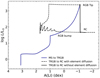 |
Fig. 1. Evolution of Li on the stellar surface for the 1 M⊙ model. The x-axis is the Li abundance. The y-axis represents the logarithm of luminosity. The lines indicate the evolution process of Li abundance. |
Almost all explanations proposed for Li-rich giants involve the He flash (Kumar et al. 2020; Mori et al. 2021; Schwab 2020). Based on the standard model of stellar structure and evolution, the He-core burning occurs when the mass of the He core increases to MHe ≈ 0.45 M⊙ (Thomas 1967; Bildsten et al. 2012). Therefore, the stellar evolution in this work was divided into two stages: Stage I is from the MS stage to MHe = 0.45 M⊙. The next range until the RC stage is called Stage II.
Figure 1 displays the evolution trajectory of the Li abundance on the surface of a 1 M⊙ star without and with element diffusion. As shown by the solid dark-blue line, the evolution of the Li abundance in both models was similar during Stage I. In the MS phase, the Li abundance is kept constant. When a low-mass star evolves into a red giant, it undergoes the first dredge-up. After the first dredge-up, Li starts to rapidly decrease because the Li elements are mixed up with the stellar interior material by the envelope deepening process and then are diluted. This depletion is due to dilution as the envelope deepens and mixes up interior material heavily depleted in Li. Before the TRGB, the Li abundance continued to drop due to the thermohaline mixing. From the ZAMS to the TRGB, the Li abundance on the stellar surface decreased by about four orders of magnitudes, which is consistent with the results of Kumar et al. (2020).
The He flash emerges on the TRGB. The Li abundance in the model without element diffusion was falling during Stage II. However, the A(Li) in the case of element diffusion increased from −1 to 1.8 dex. This indicates that element diffusion can enhance the Li abundance on the stellar surface. The main reason for this phenomenon is depicted in Fig. 2. In particular, a compact He core is formed at the TRGB, whose strong gravity can produce efficient element diffusion, resulting in the expansion of the thermohaline mixing zone. As shown in the top right panel of Fig. 2, for the model with element diffusion, the thermohaline mixing zone connected to the convection zone in the stellar interior in which the He flash occurred, that is, it extended to the deeper interior of the hydrogen-burning region. Therefore, the large amounts of 7Be, produced by the H-burning shell, could be transferred to the stellar surface, finally turning into 7Li. On the other hand, for the model without element diffusion, 7Be could not or rarely be brought to the stellar envelope due to the disconnection of the stellar interior convection zone and the thermohaline mixing zone.
 |
Fig. 2. Profiles of element abundances (top left corner) and diffusion coefficients (top right corner) (Dmix) at the first He flash. The solid lines are for the model with element diffusion, and the dashed lines are for model without element diffusion. The left and right panels at the bottom show the relative changes between the mean molecular weights (μdiff and μ) with and without element diffusion, and between the mean molecular weight gradients (∇μdiff and ∇μ) with and without element diffusion, respectively. |
Thermohaline convection is a turbulent mixing process that can occur in stellar radiative regions whenever the mean molecular weight increases with radius. In some cases, it can have a significant observable impact on stellar structure and evolution (Ulrich 1972; Kippenhahn et al. 1980; Brown et al. 2013; Garaud 2018). The left and right panels at the bottom of Fig. 2 show the relative changes in mean molecular weights (μdiff and μ) and mean molecular weight gradients (∇μdiff and ∇μ), respectively, at the junction zone between the stellar envelope and the He core. It can be seen that due to the influence of element diffusion, the μdiff and ∇μdiff have decreased significantly. The local decrease in the mean molecular weight can drive a more efficient thermohaline mixing. It expands to the inner convection region of stars, which is shown by pink lines in the top right panel. These indicate that element diffusion can greatly affect the mean molecular weight and the mean molecular weight gradient, which leads to the expansion of the mixing region of thermohaline convection.
The essence of this phenomenon is that the element diffusion mainly triggered by the gravity field suppresses the mean molecular weight and changes the element concentration gradient at the junction zone between the stellar envelope and the He core. It is one of the most important factors that affect the thermohaline mixing. It is well known that the mean molecular weight greatly affects the efficiency and range of thermohaline mixing, and makes the thermohaline mixing region expand to the inner convection region of stars; the thermohaline mixing can occur in the internal area of hydrogen burning, and bring products and by-products of nuclear reactions to the surface. Thus, a transport channel, efficiently transporting 7Be in the hydrogen-burning region of the star to the convective envelope where 7Be decays into 7Li, is formed. Although A(Li) on the surface of the star predicted by the model with element diffusion can increase to about 1.8 dex, it cannot explain the formation of the super Li-rich giants.
3.2. Effect of element diffusion with constant diffusive coefficients
According to Fig. 2, the diffusive coefficient is a very important factor for the formation of the Li-rich giant. Very recently, in order to produce the Li-rich giant, Schwab (2020) considered that turbulent convective motions can excite internal gravity waves, and a chemical mixing occurs when the luminosity of the He flash (LHe) is higher than 104 L⊙. In particular, the effective diffusive mixing coefficient was estimated to be about 1011 cm2 s−1. Given the constant diffusive mixing coefficients Dmix of 1010, 1012, and 1014 cm2 s−1 from different models, the maximum value of A(Li) calculated by Schwab (2020) was about 3.6 dex. Meanwhile, the model proposed by Schwab (2020) fails to explain the origin of super Li-rich giants.
In this section, combining the element diffusion and constant diffusive mixing coefficients, we calculate the evolution of A(Li) on the stellar surface. Following Schwab (2020), we assumed a constant diffusive mixing coefficient for the mixing when LHe > 104 L⊙. According to Fig. 2, Dmix during the He flash could reach 1015 cm2 s−1. Therefore, in this work, Dmix = 1011, 1012, 1013, and 1015 cm2 s−1 were adopted in different models.
Figure 3 displays the A(Li) evolution on the surface of a star with the mass of 1 M⊙. Using the model with a constant diffusive mixing coefficient of 1012 cm2 s−1 but without element diffusion could enhance the Li abundance up to about 1.0 dex, which agrees with the result of Schwab (2020). In the model with element diffusion, the Li abundance could be increased to 1.8 dex. At this time, the inner convection region was connected with the thermohaline mixing zone to form a channel for transporting 7Be elements, which greatly increased the 7Li on the stellar surface. Surprisingly, the model combining element diffusion and the constant diffusive mixing coefficient exhibited an increase in the A(Li) to 3.4 dex. The reason for this is that the diffusive mixing coefficient improves the mixing efficiency of the channel excited by the element diffusion. Therefore, A(Li) in the model with element diffusion and the constant diffusive mixing coefficient can keep a constant value above 3.0 dex.
3.3. Li-rich giants and super Li-rich giants
In recent years, many large survey programs have revealed the existence of numerous Li-rich giants. Combining the astrometric data from the Gaia satellite (Gaia Collaboration 2016) with spectroscopic abundance surveys (such as the GALAH survey and the LAMOST survey), twenty Li-rich abundances could be identified. Based on the GALAH DR2 and DR3 surveys, Deepak & Reddy (2019), Deepak et al. (2020), Kumar et al. (2020), and Martell et al. (2021) measured the Li abundances of 1872 giant stars. Using the LAMOST survey, Casey et al. (2019), Singh et al. (2019), and Yan et al. (2021) explored the Li abundances of more than 2000 giant stars. In order to compare the theoretical results with observation samples in this work, we selected 351 published Li-rich giants with precise values of luminosity, temperature, and Li abundance as our samples (see Table 1).
From about 11 000 observational samples, the 351 Li-rich giant stars whose luminosities are measured were selected in this work.
Figure 4 depicts the observed data on Li-rich giants and the theoretical results for the models with different values of Dmix and different masses. In this study, an increase in Dmix from 1011 to 1015 cm2 s−1 led to a rise in the A(Li) from 2.4 to 4.5 dex. For the models with element diffusion and Dmix > 1012 cm2 s−1, the evolutionary tracks passed through most of the observed samples of super Li-rich giants (A(Li) ≥ 3.2 dex) and Li-rich giants (A(Li ≥ 1.5 dex) to the normal giants. In particular, the value of A(Li) calculated in the model with element diffusion and Dmix = 1015 cm2 s−1 reached 4.5 dex, which could explain the Li abundance of the most super Li-rich giants.
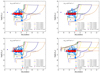 |
Fig. 4. Similar to Fig. 1, but for the models with different masses and constant diffusive mixing coefficients of Dmix to 1011 cm2 s−1, 1012 cm2 s−1, 1013 cm2 s−1, and 1015 cm2 s−1. Different values are displayed in the upper left corner of each subgraph. The solid and dashed lines show the evolutional tracks at Stages I and II, respectively. The red and blue circles are the Li-rich giant stars and the RC stars listed in Table 1, respectively. The star represents the most Li-rich giant star, TYC 429-2097-1, observed by Yan et al. (2018). |
3.4. Population synthesis for Li-rich giants
As mentioned in the Introduction, the Li-rich giants among giants are scarce (about 0.2−2%). Based on the models in this work, we estimated the theoretical ratio using the population synthesis method, which has been used in previous investigations by our group (Lü et al. 2006, 2009, 2013; Lü et al. 2020; Yu et al. 2019, 2021; Zhu et al. 2021).
In the population synthesis method for single-star systems, the initial mass function (IMF) is the most important input parameter. The IMF used in the present research was derived from the stellar distribution toward both Galactic poles, as well as that within 5.2 pc of the Sun by Kroupa et al. (1993). Based on this IMF, 106 stars were produced by a Monte Carlo calculation. In order to estimate their percentage, the lifetimes of Li-rich giants and giants were estimated afterward.
Figure 5 displays the evolution of the A(Li) in all models. After the first He flash, the element diffusion firstly initiates and enhances the Li abundance. According to Schwab (2020), the constant diffusive mixing coefficient can work when LHe > 104 L⊙. The Li abundance greatly increases after about 0.2 Myr from the first He flash, and remains constant within several Myr due to a constant Dmix. This result is proportional to the lithium depletion timescale in Casey et al. (2019). Of course, the A(Li) decreases when the stellar luminosity is lower than 104 L⊙. When the mass is greater than about 1.9 M⊙, the element diffusion and constant diffusive mixing coefficient are not excited because the temperature within the stellar envelope is too high. Simultaneously, the lifetimes of the Li-rich giants decrease with the increase in Dmix. The main reason for this is that the high diffusive coefficient accelerates the circulation process of elements, so that Be or Li elements can be quickly carried to a high-temperature zone and destroyed.
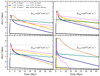 |
Fig. 5. Evolution of A(Li) after the first He flash with time. The solid lines represent the increase produced with element diffusion and different constant diffusive coefficients (Dmix). The dotted lines indicate the A(Li) of ∼1.5 dex and the A(Li) of ∼3.2 dex. |
In this study, MESA was applied to calculate the evolution of stars with initial masses of 0.9 M⊙, 1.0 M⊙, 1.2 M⊙, 1.4 M⊙, 1.6 M⊙, and 1.8 M⊙. Through a linear interpolation method, the lifetimes of Li-rich giants and giants for these 106 stars were estimated. Then, the percentage of Li-rich giants among giants was assessed. In particular, the ratio values of models with Dmix = 1011, 1012, 1013, and 1015 cm2 s−1 were 0.5, 1.2, 1.1, and 0.2%, respectively, which is consistent with the observational estimates.
Very recently, Zhang et al. (2021) has shown that the deterioration of Li in the RC stage is not so obvious and the low ratio (e.g. 0.2%) may be an anomaly. If it is true, the high diffusive coefficient (e.g. 1015 cm2 s−1) may be undesirable. It means that the model proposed in this study fails to produce all super Li-rich giants, especially the most Li-rich giant star TYC 429-2097-1. Thus, the binary merging model proposed by Zhang et al. (2020) may be competitive.
4. Conclusions
Considering the element diffusion, we used MESA to calculate the evolution of Li abundance. The element diffusion mainly triggered by the gravity field suppresses the mean molecular weight and changes the element concentration gradient at the junction zone between the stellar envelope and the He core. The local decrease in the mean molecular weight greatly affects the efficiency and range of thermohaline mixing, and makes the thermohaline mixing region expand to the inner convection region of stars. A transport channel, efficiently transporting 7Be in the hydrogen-burning region of the star to the convective envelope where 7Be decays into 7Li, is formed. Therefore, a large amount of 7Be, produced by the He flash, could be transferred to the stellar surface, finally turning into 7Li. However, the value of A(Li) could only be increased to 1.8 dex at maximum, which was insufficient to produce super Li-rich giant stars.
In turn, combining the element diffusion and constant diffusive mixing coefficients enabled us to increase the theoretical A(Li) values from 2.4 to 4.5 dex by increasing Dmix from 1011 to 1015 cm2 s−1. This means that the element diffusion in the proposed model can result in the extension of the thermohaline mixing zone and its connection with the stellar interior convection zone. Then, 7Be produced by He burning can be mixed in the stellar envelope. The high diffusive mixing coefficient can improve the efficiency of 7Be transfer to the stellar surface. Therefore, our model can produce the Li-rich giants, and even the most of super Li-rich giants. The results provided using the population synthesis method were also consistent with the observations, which confirmed the feasibility of this mechanism. However, the accuracy of the results in the model under consideration may be affected by the uncertain input parameter, Dmix. Since calculating an accurate Dmix is beyond the scope of this work, attention is rather paid to the diffusive mixing coefficients.
Here, A(Li) is the Li abundance expressed as A(Li) = log [n (Li)/n (H)] + 12, where n (Li) and n (H) are the number densities of Li and hydrogen, respectively.
Acknowledgments
We are grateful to anonymous referee for careful reading of the paper and constructive criticism. This work received the generous support of the National Natural Science Foundation of China, project Nos. U2031204, 11863005, 12163005, and 12090044, the science research grants from the China Manned Space Project with NO. CMS-CSST-2021-A10, and the Natural Science Foundation of Xinjiang No. 2021D01C075.
References
- Alastuey, A., & Jancovici, B. 1978, ApJ, 226, 1034 [NASA ADS] [CrossRef] [Google Scholar]
- Asplund, M., Grevesse, N., Sauval, A. J., & Scott, P. 2009, ARA&A, 47, 481 [NASA ADS] [CrossRef] [Google Scholar]
- Bildsten, L., Paxton, B., Moore, K., & Macias, P. J. 2012, ApJ, 744, L6 [NASA ADS] [CrossRef] [Google Scholar]
- Brown, J. A., Sneden, C., Lambert, D. L., & Dutchover, E., Jr. 1989, ApJS, 71, 293 [NASA ADS] [CrossRef] [Google Scholar]
- Brown, J. M., Garaud, P., & Stellmach, S. 2013, ApJ, 768, 34 [NASA ADS] [CrossRef] [Google Scholar]
- Buder, S., Asplund, M., Duong, L., et al. 2018, MNRAS, 478, 4513 [Google Scholar]
- Burgers, J. M. 1969, Flow Equations for Composite Gases (New York: Academic Press) [Google Scholar]
- Cameron, A. G. W. 1955, ApJ, 121, 144 [NASA ADS] [CrossRef] [Google Scholar]
- Cameron, A. G. W., & Fowler, W. A. 1971, ApJ, 164, 111 [NASA ADS] [CrossRef] [Google Scholar]
- Casey, A. R., Ruchti, G., Masseron, T., et al. 2016, MNRAS, 461, 3336 [NASA ADS] [CrossRef] [Google Scholar]
- Casey, A. R., Ho, A. Y. Q., Ness, M., et al. 2019, ApJ, 880, 125 [Google Scholar]
- Charbonnel, C., & Zahn, J. P. 2007, A&A, 467, L15 [NASA ADS] [CrossRef] [EDP Sciences] [Google Scholar]
- Cyburt, R. H., Amthor, A. M., Ferguson, R., et al. 2010, ApJS, 189, 240 [NASA ADS] [CrossRef] [Google Scholar]
- Deepak, & Reddy, B. E. 2019, MNRAS, 484, 2000 [NASA ADS] [Google Scholar]
- Deepak, Lambert, D. L., & Reddy, B. E. 2020, MNRAS, 494, 1348 [Google Scholar]
- Dupuis, J., Fontaine, G., Pelletier, C., & Wesemael, F. 1992, ApJS, 82, 505 [NASA ADS] [CrossRef] [Google Scholar]
- Ferguson, J. W., Alexander, D. R., Allard, F., et al. 2005, ApJ, 623, 585 [Google Scholar]
- Gaia Collaboration 2018, VizieR Online Data Catalog: I/345 [Google Scholar]
- Gaia Collaboration (Prusti, T., et al.) 2016, A&A, 595, A1 [NASA ADS] [CrossRef] [EDP Sciences] [Google Scholar]
- Gao, Q., Shi, J.-R., Yan, H.-L., et al. 2019, ApJS, 245, 33 [NASA ADS] [CrossRef] [Google Scholar]
- Garaud, P. 2018, Annu. Rev. Fluid Mech., 50, 275 [NASA ADS] [CrossRef] [Google Scholar]
- Holanda, N., Drake, N. A., & Pereira, C. B. 2020, AJ, 159, 9 [Google Scholar]
- Iben, I., Jr. 1967a, ApJ, 147, 650 [NASA ADS] [CrossRef] [Google Scholar]
- Iben, I., Jr. 1967b, ApJ, 147, 624 [NASA ADS] [CrossRef] [Google Scholar]
- Iglesias, C. A., & Rogers, F. J. 1993, ApJ, 412, 752 [Google Scholar]
- Iglesias, C. A., & Rogers, F. J. 1996, ApJ, 464, 943 [NASA ADS] [CrossRef] [Google Scholar]
- Itoh, N., Totsuji, H., Ichimaru, S., & Dewitt, H. E. 1979, ApJ, 234, 1079 [NASA ADS] [CrossRef] [Google Scholar]
- Kippenhahn, R., Ruschenplatt, G., & Thomas, H. C. 1980, A&A, 91, 175 [Google Scholar]
- Kirby, E. N., Guhathakurta, P., Zhang, A. J., et al. 2016, VizieR Online Data Catalog: J/ApJ/819/135 [Google Scholar]
- Kroupa, P., Tout, C. A., & Gilmore, G. 1993, MNRAS, 262, 545 [NASA ADS] [CrossRef] [Google Scholar]
- Kumar, Y. B., Reddy, B. E., & Lambert, D. L. 2011, ApJ, 730, L12 [NASA ADS] [CrossRef] [Google Scholar]
- Kumar, Y. B., Reddy, B. E., Campbell, S. W., et al. 2020, Nat. Astron., 4, 1059 [NASA ADS] [CrossRef] [Google Scholar]
- Lattanzio, J. C., Siess, L., Church, R. P., et al. 2015, MNRAS, 446, 2673 [CrossRef] [Google Scholar]
- Li, H., Aoki, W., Matsuno, T., et al. 2018, ApJ, 852, L31 [NASA ADS] [CrossRef] [Google Scholar]
- Lind, K., Primas, F., Charbonnel, C., Grundahl, F., & Asplund, M. 2009, A&A, 503, 545 [NASA ADS] [CrossRef] [EDP Sciences] [Google Scholar]
- Liu, Y. J., Tan, K. F., Wang, L., et al. 2014, ApJ, 785, 94 [NASA ADS] [CrossRef] [Google Scholar]
- Lodders, K. 2019, Nuclei in the Cosmos XV (Cham: Springer International Publishing) [Google Scholar]
- Lü, G., Yungelson, L., & Han, Z. 2006, MNRAS, 372, 1389 [CrossRef] [Google Scholar]
- Lü, G., Zhu, C., Wang, Z., & Wang, N. 2009, MNRAS, 396, 1086 [CrossRef] [Google Scholar]
- Lü, G., Zhu, C., & Podsiadlowski, P. 2013, ApJ, 768, 193 [CrossRef] [Google Scholar]
- Lü, G., Zhu, C., Wang, Z., et al. 2020, ApJ, 890, 69 [CrossRef] [Google Scholar]
- Martell, S. L., & Shetrone, M. D. 2013, MNRAS, 430, 611 [NASA ADS] [CrossRef] [Google Scholar]
- Martell, S. L., Simpson, J. D., Balasubramaniam, A. G., et al. 2021, MNRAS, 505, 5340 [NASA ADS] [Google Scholar]
- Monaco, L., Villanova, S., Moni Bidin, C., et al. 2011, A&A, 529, A90 [NASA ADS] [CrossRef] [EDP Sciences] [Google Scholar]
- Mori, K., Kusakabe, M., Balantekin, A. B., Kajino, T., & Famiano, M. A. 2021, MNRAS, 503, 2746 [NASA ADS] [CrossRef] [Google Scholar]
- Paquette, C., Pelletier, C., Fontaine, G., & Michaud, G. 1986, ApJS, 61, 177 [Google Scholar]
- Paxton, B., Bildsten, L., Dotter, A., et al. 2011, ApJS, 192, 3 [Google Scholar]
- Paxton, B., Cantiello, M., Arras, P., et al. 2013, ApJS, 208, 4 [Google Scholar]
- Paxton, B., Marchant, P., Schwab, J., et al. 2015, ApJS, 220, 15 [Google Scholar]
- Paxton, B., Schwab, J., Bauer, E. B., et al. 2018, ApJS, 234, 34 [NASA ADS] [CrossRef] [Google Scholar]
- Paxton, B., Smolec, R., Schwab, J., et al. 2019, ApJS, 243, 10 [Google Scholar]
- Reimers, D. 1975, Mem. Soc. R. Sci. Liege, 8, 369 [NASA ADS] [Google Scholar]
- Rogers, F. J., & Nayfonov, A. 2002, ApJ, 576, 1064 [Google Scholar]
- Ruchti, G. R., Fulbright, J. P., Wyse, R. F. G., et al. 2011, ApJ, 743, 107 [Google Scholar]
- Schwab, J. 2020, ApJ, 901, L18 [NASA ADS] [CrossRef] [Google Scholar]
- Semenova, E., Bergemann, M., Deal, M., et al. 2020, A&A, 643, A164 [NASA ADS] [CrossRef] [EDP Sciences] [Google Scholar]
- Simonucci, S., Taioli, S., Palmerini, S., & Busso, M. 2013, ApJ, 764, 118 [NASA ADS] [CrossRef] [Google Scholar]
- Singh, R., Reddy, B. E., Bharat Kumar, Y., & Antia, H. M. 2019, ApJ, 878, L21 [NASA ADS] [CrossRef] [Google Scholar]
- Singh, R., Reddy, B. E., Campbell, S. W., Kumar, Y. B., & Vrard, M. 2021, ApJ, 913, L4 [NASA ADS] [CrossRef] [Google Scholar]
- Smiljanic, R., Franciosini, E., Bragaglia, A., et al. 2018, A&A, 617, A4 [NASA ADS] [CrossRef] [EDP Sciences] [Google Scholar]
- Stanton, L. G., & Murillo, M. S. 2016, Phys. Rev. E, 93, 043203 [NASA ADS] [CrossRef] [Google Scholar]
- Stephan, A. P., Naoz, S., & Gaudi, B. S. 2018, AJ, 156, 128 [NASA ADS] [CrossRef] [Google Scholar]
- Thomas, H. C. 1967, in Late-Type Stars, ed. M. Hack, 395 [Google Scholar]
- Thoul, A. A., Bahcall, J. N., & Loeb, A. 1994, ApJ, 421, 828 [Google Scholar]
- Timmes, F. X., & Swesty, F. D. 2000, ApJS, 126, 501 [NASA ADS] [CrossRef] [Google Scholar]
- Ulrich, R. K. 1972, ApJ, 172, 165 [NASA ADS] [CrossRef] [Google Scholar]
- Vescovi, D., Piersanti, L., Cristallo, S., et al. 2019, A&A, 623, A126 [NASA ADS] [CrossRef] [EDP Sciences] [Google Scholar]
- Wallerstein, G., & Sneden, C. 1982, ApJ, 255, 577 [NASA ADS] [CrossRef] [Google Scholar]
- Yan, H.-L., Shi, J.-R., Zhou, Y.-T., et al. 2018, Nat. Astron., 2, 790 [NASA ADS] [CrossRef] [Google Scholar]
- Yan, H.-L., Zhou, Y.-T., Zhang, X., et al. 2021, Nat. Astron., 5, 86 [NASA ADS] [CrossRef] [Google Scholar]
- Yu, J., Li, Z., Zhu, C., et al. 2019, ApJ, 885, 20 [NASA ADS] [CrossRef] [Google Scholar]
- Yu, J., Zhang, X., & Lü, G. 2021, MNRAS, 504, 2670 [NASA ADS] [CrossRef] [Google Scholar]
- Zhang, X., Jeffery, C. S., Li, Y., & Bi, S. 2020, ApJ, 889, 33 [NASA ADS] [CrossRef] [Google Scholar]
- Zhang, J., Shi, J.-R., Yan, H.-L., et al. 2021, ApJ, 919, L3 [NASA ADS] [CrossRef] [Google Scholar]
- Zhu, C., Liu, H., Wang, Z., & Lü, G. 2021, A&A, 654, A57 [NASA ADS] [CrossRef] [EDP Sciences] [Google Scholar]
All Tables
From about 11 000 observational samples, the 351 Li-rich giant stars whose luminosities are measured were selected in this work.
All Figures
|
Fig. 1. Evolution of Li on the stellar surface for the 1 M⊙ model. The x-axis is the Li abundance. The y-axis represents the logarithm of luminosity. The lines indicate the evolution process of Li abundance. |
| In the text | |
|
Fig. 2. Profiles of element abundances (top left corner) and diffusion coefficients (top right corner) (Dmix) at the first He flash. The solid lines are for the model with element diffusion, and the dashed lines are for model without element diffusion. The left and right panels at the bottom show the relative changes between the mean molecular weights (μdiff and μ) with and without element diffusion, and between the mean molecular weight gradients (∇μdiff and ∇μ) with and without element diffusion, respectively. |
| In the text | |
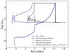 |
Fig. 3. Similar to Fig. 1, but for the evolutional tracks of Li abundances of four models. |
| In the text | |
|
Fig. 4. Similar to Fig. 1, but for the models with different masses and constant diffusive mixing coefficients of Dmix to 1011 cm2 s−1, 1012 cm2 s−1, 1013 cm2 s−1, and 1015 cm2 s−1. Different values are displayed in the upper left corner of each subgraph. The solid and dashed lines show the evolutional tracks at Stages I and II, respectively. The red and blue circles are the Li-rich giant stars and the RC stars listed in Table 1, respectively. The star represents the most Li-rich giant star, TYC 429-2097-1, observed by Yan et al. (2018). |
| In the text | |
|
Fig. 5. Evolution of A(Li) after the first He flash with time. The solid lines represent the increase produced with element diffusion and different constant diffusive coefficients (Dmix). The dotted lines indicate the A(Li) of ∼1.5 dex and the A(Li) of ∼3.2 dex. |
| In the text | |
Current usage metrics show cumulative count of Article Views (full-text article views including HTML views, PDF and ePub downloads, according to the available data) and Abstracts Views on Vision4Press platform.
Data correspond to usage on the plateform after 2015. The current usage metrics is available 48-96 hours after online publication and is updated daily on week days.
Initial download of the metrics may take a while.