| Issue |
A&A
Volume 696, April 2025
|
|
|---|---|---|
| Article Number | A78 | |
| Number of page(s) | 37 | |
| Section | Extragalactic astronomy | |
| DOI | https://doi.org/10.1051/0004-6361/202450963 | |
| Published online | 04 April 2025 | |
A Virgo Environmental Survey Tracing Ionised Gas Emission (VESTIGE)
XVII. Statistical properties of individual H II regions in unperturbed systems⋆
1
Aix Marseille Univ, CNRS, CNES, LAM, Marseille, France
2
Universitá di Milano-Bicocca, piazza della scienza 3, 20100 Milano, Italy
3
INAF – Osservatorio Astronomico di Brera, Via Brera 28, 20121 Milano, Italy
4
Université Côte d’Azur, Observatoire de la Côte d’Azur, CNRS, Laboratoire Lagrange, 06000 Nice, France
5
Laboratoire d’Astrophysique de Bordeaux, Univ. Bordeaux, CNRS, B18N, allée Geoffroy Saint-Hilaire, 33615 Pessac, France
6
National Research Council of Canada, Herzberg Astronomy and Astrophysics, 5071 West Saanich Road, Victoria, BC V9E 2E7, Canada
7
AIM, CEA, CNRS, Université Paris-Saclay, Université Paris Diderot, Sorbonne Paris Cité, Observatoire de Paris, PSL University, F-91191 Gif-sur-Yvette Cedex, France
8
Department of Astrophysics, University of Vienna, Türkenschanzstrasse 17, 1180 Vienna, Austria
9
INAF – Osservatorio Astronomico di Brera, Via Brera 28, 20121 Milano, Italy
10
Institut Universitaire de France, 1 rue Descartes, 75005 Paris, France
⋆⋆ Corresponding author; This email address is being protected from spambots. You need JavaScript enabled to view it.
Received:
2
June
2024
Accepted:
14
February
2025
Abstract
The Virgo Environmental Survey Tracing Ionised Gas Emission (VESTIGE) survey is a blind narrow-band Hα + [N II] imaging survey of the Virgo cluster carried out with MegaCam of the Canada-France-Hawaii Telescope. The survey provides deep narrow-band images for 385 galaxies hosting star-forming H II regions. We identify individual H II regions and measure their main physical properties such as Hα luminosity, equivalent diameter, and electron density with the purpose of deriving standard relations that can serve as a reference for future local and high-z studies of H II regions in star-forming systems in different environments. For this purpose, we used a complete sample of ≃13.000 H II regions of luminosity L(Hα)≥1037 erg s−1 in order to derive the main statistical properties of H II regions in unperturbed systems, which are identified as those galaxies with a normal H I gas content, and are in total 64 objects. These are the composite Hα luminosity function, equivalent diameter and electron density distribution, and luminosity-size relation. We also derived the main scaling relations between several parameters representative of the H II regions (total number, luminosity of the first ranked regions, fraction of the diffuse component, best-fit parameters of the Schechter luminosity function measured for individual galaxies) and those characterising the properties of the host galaxies (stellar mass, star formation rate and specific star formation rate, stellar mass and star formation rate surface density, metallicity, molecular-to-atomic gas ratio, total gas-to-dust mass ratio). We briefly discuss the results of this analysis and their implications in the study of the star formation process in galaxy discs.
Key words: galaxies: star formation
Based on observations obtained with MegaPrime/MegaCam, a joint project of CFHT and CEA/DAPNIA, at the Canada-France-Hawaii Telescope (CFHT) which is operated by the National Research Council (NRC) of Canada, the Institut National des Sciences de l’Univers of the Centre National de la Recherche Scientifique (CNRS) of France and the University of Hawaii.
Scientific associate INAF – Osservatorio Astronomico di Cagliari, Via della Scienza 5, 09047 Selargius (CA), Italy.
© The Authors 2025
 Open Access article, published by EDP Sciences, under the terms of the Creative Commons Attribution License (https://creativecommons.org/licenses/by/4.0), which permits unrestricted use, distribution, and reproduction in any medium, provided the original work is properly cited.
This article is published in open access under the Subscribe to Open model. This email address is being protected from spambots. You need JavaScript enabled to view it. to support open access publication.
1. Introduction
The process responsible for the transformation of the cold gas distributed within the interstellar medium (ISM) of galaxies into new stars is one of the most studied phenomena in astronomy. Its importance resides in the fact that this process governs the transformation of the primordial baryonic component, atomic hydrogen, into galaxies, and it is thus at the origin of galaxy evolution. If at kiloparsec scales the transformation of the gas along the disc of galaxies mainly follows the Schmidt relation, where the star formation surface density is proportionally related to the cold gas column density (e.g. Schmidt 1959; Kennicutt 1998; Bigiel et al. 2008; Kennicutt & Evans 2012), at smaller scales, the formation of stars takes place within giant molecular clouds (GMCs). Stars are formed here within compact regions generally called H II regions, where the hard stellar radiation produced by the youngest (O, early-B) and most massive (≳10 M⊙, e.g. Kennicutt 1998) stars is sufficiently energetic to ionise the surrounding gas. These star-forming regions are easily identified thanks to their emission in several hydrogen lines. The strongest of these that is visible in the optical domain is Hα at 6563 Å (Balmer line).
Although the star formation process at the scale of GMCs has been the topic of hundreds of past and recent studies, many open questions remain unanswered. The main difficulty in understanding this phenomenon resides in the fact that several competitive mechanisms (gravity, turbulence, different kinds of instabilities, gas cooling and heating in a multiphase and mixed medium, confinement in magnetic fields, external pressure, shocks, etc.) act simultaneously. Still unclear are the initial conditions necessary for the gas to collapse into molecular clouds, in particular within those located along filaments; how the molecular clouds collapse and fragment into clumps where stars are formed with the typical distribution characterised by the initial stellar mass function (IMF); and the efficiency at which this occurs (e.g. Shu et al. 1987; McKee & Ostriker 2007; Dobbs et al. 2014; Inutsuka et al. 2015; Chevance et al. 2020a,b). It is clear that the star formation process depends on several factors acting at different scales, from gas infall from the intergalactic medium into the disc (megaparsec scales) down to the fragmentation of the molecular gas within GMCs into clumps and cores (1–0.1 pc scales; e.g. Kennicutt & Evans 2012). At the scale of galactic discs, the process of star formation can depend on several factors, including the aforementioned gas column density (Schmidt law), possibly modulated by the rotational velocity of the disc (Wyse & Silk 1989; Boissier et al. 2001); the stellar mass density of the disc (Shi et al. 2018); the dynamical time (Silk 1997; Elmegreen 2000) or the free-fall time on the cloud (Krumholz et al. 2012); the presence of spiral density waves; the metallicity of the gas and its molecular-to-atomic fraction; and the dust content and distribution (e.g. Dey et al. 2019). All of these parameters are known to scale with the intrinsic size and mass of the host galaxies (scaling relations, e.g. Gavazzi et al. 1996; Boselli et al. 2001, 2014a; Tremonti et al. 2004; Cortese et al. 2012; Saintonge & Catinella 2022), it is thus interesting to investigate how parameters representative of the star formation process at scales of individual H II regions scale as a function of other parameters indicative of global galaxy properties such as morphological type, stellar mass, star formation rate, metallicity, and gas and dust content. The same properties might also change in hostile environments, such as clusters and groups, where different kinds of perturbations are known to modify the star formation process at large scales (star formation quenching; Boselli & Gavazzi 2006; Peng et al. 2010).
The Virgo Environmental Survey Tracing Ionised Gas Emission (VESTIGE) is a blind Hα narrow-band (NB) imaging survey of the Virgo cluster carried out at the Canada-France-Hawaii Telescope (CFHT) at Maunakea (Boselli et al. 2018a). Designed to cover the full cluster up to its virial radius at unprecedented depth and angular resolution, the survey has detected almost four hundred star-forming galaxies, some of which are still unperturbed by the hostile cluster environment (Boselli et al. 2023a). The spectacular image quality of the data and their sensitivity allow us to identify thousands of individual H II regions in most of these objects, all of which are located at about the same distance, and thus study in detail their statistical properties on a complete and homogeneous sample. The properties of the H II regions identified in a few representative objects have already been presented in dedicated works (the perturbed galaxy IC 3476, Boselli et al. 2021; lenticular galaxies, Boselli et al. 2022a). Those of a statistically significant sample of mainly perturbed systems have been discussed in Boselli et al. (2020). The main purpose of this work is to derive the main statistical properties (e.g. composite distributions and scaling relations) of a large sample of unperturbed systems mainly located at the periphery of the cluster. Most of these relations have already been derived, studied, and interpreted in dedicated works based on very local samples including only a handful of galaxies (Kennicutt et al. 1989a,b) or otherwise composed of more distant objects with limited data quality (Caldwell et al. 1991; Banfi et al. 1993; Rozas et al. 1996a; Elmegreen & Salzer 1999; Beckman et al. 2000; Thilker et al. 2002; Helmboldt et al. 2005; Bradley et al. 2006). The most recent study used spectacular NB imaging data in the near-IR domain gathered with the Hubble Space telescope (HST; Liu et al. 2013), where the exquisite angular resolution allowed the authors to resolve H II regions down to scales of ∼10–20 pc. Another recent work is based on data obtained by the Very Large Telescope (VLT) with the Multi Unit Spectroscopic Explorer (MUSE) during the Physics at High Angular Resolution in Nearby Galaxies (PHANGS) survey and has the advantage of being based on integral field unit (IFU) spectroscopic data, which is of primordial importance to infer the physical properties of the identified star-forming regions (Santoro et al. 2022). Both works, however, are limited in statistics, with the former including only 12 objects and the latter 19, and in the sampling of the galaxy parameter space, which is mainly limited to massive systems (Mstar ≳ 109.4 − 10 M⊙). The sample analysed in this work includes 64 galaxies; spans a wide range in morphological type – dE, S0, spirals, Magellanic irregulars, blue compact dwarfs (BCDs) – and stellar mass (107 ≲ Mstar ≲ 1011 M⊙); and has ≃13.000 H II regions of luminosity L(Hα)≥1037 erg s−1. The spectacular imaging quality of the data gathered at the CFHT (full-width-half-maximum FWHM ≃ 0.7″) allows us to resolve H II regions down to ≃60 pc. It is thus ideally designed to trace the main statistical properties of H II regions located in normal unperturbed star-forming galaxies in the local Universe and thus provides a benchmark reference for future local and high redshift studies. As designed, the VESTIGE survey also covers hundreds of perturbed systems located within the inner regions of the cluster, which are ideal targets to study the effects of the different kinds of perturbations on the star formation process down to the scale of individual H II regions. The sample analysed in this work and based on the same set of data will also be an ideal reference for a comparative study between perturbed and unperturbed objects, which will be presented in a forthcoming publication.
This paper is structured as follows: In Sect. 2 we describe the sample, and in Sect. 3, we introduce the full set of multifrequency data used for the analysis presented in Sect. 4. This includes a detail description of the composite Hα luminosity function, diameter, and electron density distribution of the detected H II regions as well as the main scaling relations. The results are compared to those already available in the literature and discussed in Sect. 5, while the conclusions are given in Sect. 6.
2. Sample
The sample of galaxies analysed in this work is composed of the star-forming objects detected during the VESTIGE survey. Out of the 385 galaxies detected in Hα, however, we exclude a few objects where the ionised gas emission is diffuse and not associated with star-forming episodes, for example in M87 (Boselli et al. 2019) or in a few bright lenticular galaxies (Boselli et al. 2022a). We also exclude nearly edge-on systems (b/a < 0.25, ∼corresponding to an inclination i ≳ 75 degrees, where a and b are the major and minor axes measured on the i-band Next Generation Virgo Survey (NGVS) images of Ferrarese et al. 2012 and available for all the targets), since the morphology prevents an accurate identification of the H II regions located along the disc. Finally, we also exclude the few H II regions located outside the optical disc (see Sect. 3.4), as observed in several systems (e.g. IC 3418, Hester et al. 2010; Fumagalli et al. 2011; NGC 4254, Boselli et al. 2018b; AGC226178, Junais et al. 2021; Jones et al. 2022; IC 3476, Boselli et al. 2021). These regions have been probably produced during the interaction of galaxies with their surrounding environment and will be studied in a dedicated work. Their exact number is still unknown given the difficulty in identifying and disentangling them from other sources (planetary nebulae, background line emitters) with consistent and homogeneous criteria on such a large region of the sky. Their number, however, is limited when compared to the number of H II within the disc of massive spirals (in NGC 4254 is ≃0.1% at the limiting luminosity of L(Hα)≥1037 erg s−1). It might be more important in dwarf, perturbed systems. In IC 3418 all H II regions are located outside the stellar disc (Hester et al. 2010; Fumagalli et al. 2011), and are thus not analysed in this work.
We then consider only those objects hosting H II regions brighter than the completeness limit of L(Hα)≥1037 erg s−1 (see Sect. 3.5). Throughout the paper, we will refer to this sample as to the parent sample. The parent sample is thus composed of 322 star-forming galaxies and is, at present, the largest sample ever studied in the literature, spanning a wide range in morphological type, from giant spirals and lenticulars to dwarf ellipticals, Magellanic irregulars, and blue compact dwarfs (BCDs), and stellar mass (107 ≲ Mstar ≲ 1011 M⊙), with an homogeneous set of NB imaging data suitable for this analysis. The exceptional quality of this sample is also related to the fact that it is composed of galaxies all at a similar distance, thus minimising distance related completeness biases. Indeed, the distance of each galaxy is here taken as the mean distance of the Virgo cluster subgroup to which the galaxy belongs. The membership to the different cluster substructures has been described in Boselli et al. (2023b). It depends on the relative distance of galaxies to the core of the different clouds and on their recessional velocity. With respect to previous works of this series, however, we assume the updated mean distance to the different substructure recently published by Cantiello et al. (2024), that is 16.5 Mpc for galaxies belonging to the main body of the cluster associated with M87 (cluster A), and to the low velocity cloud (LVC), 15.8 Mpc for galaxies in cluster B (M49) and cluster C (M60)1, 23 Mpc in the W′ cloud, and 32 Mpc for objects in the W and M clouds (see Boselli et al. 2023b for details).
To separate normal galaxies mainly following a secular evolution from those perturbed by their surrounding environment we use the H I-deficiency parameter (e.g. Boselli & Gavazzi 2006; Cortese et al. 2021; Boselli et al. 2022b). This parameter is defined as the difference (in logarithmic scale) between the expected and the observed atomic gas mass of the targeted galaxies (Haynes & Giovanelli 1984), where the expected H I mass of each object is here derived using the scaling relations of gas-rich field galaxies recently calibrated by Cattorini et al. (2023). This calibration is perfectly indicated for this sample because it includes dwarf systems such as those detected during the VESTIGE survey. H I masses or upper limits are available for all the targets (see Boselli et al. 2023a for details). In the following analysis, we consider as unperturbed systems those with an H I-deficiency parameter H I−def ≤ 0.4, in line with what was done in all previous VESTIGE publications (e.g. Boselli et al. 2020, 2023a,b; see Fig. 1). With all these criteria the parent sample is composed of 322 objects, out of which 64 unperturbed systems that will be used in this work2. We will refer to this sample of 64 objects as to the unperturbed sample. Those possibly suffering an interaction with their surrounding environment (258 objects), will be the targets of a comparative analysis which will be presented in a companion paper (perturbed sample; see Table 1).
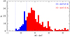 |
Fig. 1. Distribution of the H I-deficiency parameter for the parent sample galaxies. The blue histogram shows the distribution of the unperturbed systems with H I−def ≤ 0.4 and b/a ≥ 0.25 analysed in this work (64 objects, unperturbed sample), the red histogram the one of perturbed galaxies with H I−def > 0.4 and b/a ≥ 0.25 (258 objects, perturbed sample). The blue dotted vertical lines show the 1σ range distribution of the H I-deficiency parameter observed in isolated systems. |
The sample of galaxies.
3. Data
3.1. Narrow-band Hα imaging data
The data analysed in this work are extracted from the deep NB Hα images gathered during the VESTIGE survey of the Virgo cluster undertaken with MegaCam at the CFHT. The survey, which covers the Virgo cluster up to its virial radius (104 deg.2), is extensively described in Boselli et al. (2018a). The data were gathered in two filters, the NB filter MP9603 centred on the Hα line (λc = 6591 Å; Δλ = 106 Å), and the broad-band r filter necessary for the subtraction of the stellar continuum (Boselli et al. 2019). The NB filter, which includes the emission of the Hα (λ = 6563 Å) and of the two [N II] lines (λ = 6548, 6583 Å), has its peak transmissivity in the velocity range −1140 ≤ vhel ≤ 3700 km s−1 (see Boselli et al. 2018a). It is thus perfectly suited for the observations of all the galaxies at the distance of the cluster, whose redshift is included in the velocity range −300 ≤ vhel ≤ 3000 km s−1 (Boselli et al. 2014b). The data were collected thanks to several exposures using a large dither pattern to minimise any unwanted gradient in the sky background due to the reflection of bright stars possibly present in the fields. The total integration time was 2 hours in the NB filter and 12 min in the broad r-band filter. The survey is now 76% complete. Full sensitivity is reached almost everywhere within the VESTIGE footprint. A few shorter (a factor of ∼2) exposures are present at the far edges of the footprint. With these integration times the sensitivity of the survey is f(Hα)≃4 × 10⁻¹⁷ erg s−1 cm−2 (5σ) for point sources and Σ(Hα)≃2 × 10⁻¹⁸ erg s−1 cm−2 arcsec−2 (1σ after smoothing the data to ≃3″ resolution) for extended sources. The sensitivity might drop by a factor ≃1.5 at the periphery of the cluster where full depth was not always reached.
The data were reduced using Elixir-LSB (Ferrarese et al. 2012), a pipeline expressly designed to optimise the detection of extended low surface brightness features such as those produced during the interaction of galaxies with their surrounding environment. The photometric calibration (≤0.02–0.03 mag) and the astrometric corrections (≤100 mas) in both the NB Hα and broad-band r filters was secured using the same standard procedures described in Gwyn (2008) and here optimised for these filters. This is done after cross-matching several thousand of unsaturated stars in the observed frames with those available from the Panoramic Survey Telescope and Rapid Response System (Pan-STARRS). The photometric calibration in the NB Hα filter was derived after applying a colour correction to unsaturated stars in each field, a standard technique now commonly applied to wide field imaging data. This correction has been calibrated by convolving the spectra of a large sample of ≃50 000 stars of different type with available spectra in Sloian digital sky survey (SDSS) with the transmissivity curve of different CFHT filters, including the NB Hα one, and fitted with a polynomial relation as described in Gwyn (2008).
We stress that the sensitivity of the survey for point sources at the mean distance of the Virgo cluster (16.5 Mpc, Gavazzi et al. 1999; Mei et al. 2007; Blakeslee et al. 2009; Cantiello et al. 2018, see below) is L(Hα)≥1.3 × 1036 erg s−1. This luminosity is lower than the Hα luminosity expected for the emission of a single ionising O star and is comparable to that of a single early-B star (Sternberg et al. 2003). This unique set of data is thus potentially able to detect all the ionising emission of star-forming regions in the selected galaxies. As we will see in Sect. 3.4, however, the detection of all H II regions might be hampered by other factors such as confusion, the presence of contaminating stars, dust attenuation which might affect in different ways regions of different age, and the correct determination of the diffuse underlying emission. The exceptional image quality of the data, which have a mean seeing of FWHMPSF = 0.73″ in the NB filter and FWHMPSF = 0.77″ in the r-band (see Fig. 2), allows us to resolve H II regions of diameter ≳60 pc at the mean distance of the cluster (16.5 Mpc).
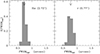 |
Fig. 2. Normalised seeing distribution in the HαNB (upper panel) and r-band (lower panel). At the distance of the Virgo cluster (16.5 Mpc), the mean values (indicated by a vertical arrow and given in parenthesis) correspond to 58 pc and 62 pc in the HαNB and r-band, respectively. |
3.2. Multifrequency data
As discussed in Boselli et al. (2023a), a complete set of multifrequency data from the far-UV to the far-IR, including NGVS u, g, i, z broad-band imaging (Ferrarese et al. 2012), is available for the target galaxies. Stellar masses are derived using a spectral energy distribution (SED) fitting analysis based on the CIGALE SED fitting code (Boquien et al. 2019) using integrated photometry. This is done assuming a Chabrier (2003) initial mass function (IMF)3. The same SED fitting code provides dust masses whenever the galaxies have been detected in a sufficient number of photometric mid- and far-IR bands. The dust masses are determined fitting the dust spectral energy distribution from 100 μm to 500 μm with the Draine et al. (2007, 2014) models. The PAH fraction qPAH is fixed at 2.5%. We let the other parameters cover the full range: Umin (minimum radiation field) from 0.1 to 50, α (defined as dU/dM ∝ U−α), and γ (the fraction of dust illuminated by a star-forming region) from 10−3 to 10−0.3. Finally, the dust mass and the related uncertainties are computed from likelihood-weighted means and standard deviations over the full parameter space.
Total Hα luminosities are extracted from the images by integrating the flux emission within elliptical regions expressly defined to include all the emitting sources associated with each galaxy. These apertures have been manually optimised to include all the diffuse emission and the H II regions located within the optical disc of each galaxy and identified on the continuum-subtracted Hα image, and at the same time minimise the sky contribution within the aperture to reduce the uncertainty on the measure. The H II regions selected within these elliptical apertures are located within the stellar extension of the galaxies as determined at the limiting surface brightness of the deep r-band images. At this surface brightness limit, the r-band extension of all galaxies is slightly larger than the one measured by Binggeli et al. (1985) at the B-band 25.5 mag arcsec−2 isophote, in particular in dwarf irregular objects with complex morphologies.
In NGC 4567, where the optical disc of the galaxy partly overlaps with the one of the nearby NGC 4568, the elliptical aperture has been manually defined to maximise the contribution of NGC 4567 and minimise that of the companion. In this particular system, both the Hα total flux and the identified H II regions might be partly contaminated by those of the companion. The same elliptical apertures are used to estimate the sky background in regions randomly placed around the galaxy, as described in Boselli et al. (2023a). Total Hα luminosities are corrected for [N II] contamination and dust attenuation using the spectroscopic data available for the parent sample, as extensively described in Boselli et al. (2023a). This includes MUSE IFU or high-quality long slit spectroscopy (Fossati et al. 2018; Boselli et al. 2018c, 2021, 2022a; 12 objects), integrated long slit spectroscopy gathered by drifting the slit of the telescope over the disc of the target galaxies (Gavazzi et al. 2004; Boselli et al. 2013, 2015; 116 objects), SDSS spectroscopy of the inner regions (114 objects), or scaling relations for the remaining (mostly dwarf) systems (142 objects), where the [N II] contamination is generally (if present) minimal (the [N II]/Hα ratio4 is < 0.2 in 60% of this subsample) and dust attenuation A(Hα) ≃ 0 (see Boselli et al. 2023a). While Balmer decrement measurements take into account any effect related to the inclination of the galaxy on the plane of the sky, the adopted scaling relation does not. We expect, however, that any second order effect related to inclination is marginal in these low-metallicity, dust-poor dwarf systems. Luminosities are then converted to star formation rates assuming a Chabrier IMF. The same set of spectroscopic data are also used to derive gas metallicities. For those galaxies with available integrated spectroscopy, metallicities are derived by Hughes et al. (2013) and calibrated on the Pettini & Pagel 2004 relation based on the [O III] λ5007 Å and [N II] λ6583 Å calibrators. For those galaxies with only SDSS spectra, metallicities have been derived consistently using both Pettini & Pagel (2004) calibrations. Metallicities are available for 39/64 of the unperturbed sample galaxies.
Finally, we derived the total gas content, defined as Mgas = 1.3 × (MHI + MH2) (the factor 1.3 is to take into account the Helium contribution), and the atomic-to-molecular gas ratio MHI/MH2 for those galaxies with available high-quality molecular gas data. These have been taken from the Virgo environment traced in CO survey (VERTICO) when available (Brown et al. 2021), or from the Herschel Reference Survey (HRS, Boselli et al. 2014c). Both sets of data have been corrected to a common and constant XCO conversion factor of XCO = 2.3 × 1020 cm−2/(K km s−1) (Strong et al. 1988). As mentioned above, H I data are available for the whole parent sample (see Boselli et al. 2023a for details), molecular masses for 15/64, and dust masses for 30/64. Gas-to-dust masses (G/D) are integrated values defined as G/D = Mgas/Mdust, and are available for 15/64 objects.
3.3. Subtraction of the stellar continuum
An accurate and unbiased subtraction of the stellar continuum is critical to measuring the emission of the ionised gas in the Hα + [N II] lines. This was done as extensively discussed in the previous VESTIGE papers (e.g. Boselli et al. 2018a, 2019). In brief, the flux density of of the stellar continuum emission at the effective wavelength of the NB filter is derived from the r-band image using the relation (Boselli et al. 2019)
![Mathematical equation: $$ \begin{aligned} {\frac{r}{\text{ H}\alpha +[{\text{ N}}\,\text{ ii}]} = r - 0.1713 \times (g{-}r) + 0.0717}, \end{aligned} $$](/articles/aa/full_html/2025/04/aa50963-24/aa50963-24-eq1.gif) (1)
(1)
where the emission in the r, g, and NB Hα + [N II] filters is expressed in AB magnitudes, and where all the images have been taken in similar and excellent seeing conditions. This colour correction has been calibrated using several thousands Milky Way stars with spectra available in the SDSS, and colours in the range 0.15 ≤ g − r ≤ 1.0 mag. The residual bias after this correction is consistent with zero with a random scatter of 0.03 mag. This colour-dependent calibration is necessary to take into account the galaxy spectral slope between the effective wavelengths of the NB and r-band filters. This procedure reduces systematic biases on the Hα + [N II] flux (Spector et al. 2012). The residual scatter in the relation is taken into account in our error budget and combines spectral calibration uncertainties as well as effects related to the age of the stars, to their metallicity, and reddening. The lack of an accurate estimate of these parameters in the calibrating stars and in the target galaxies, in particular on scales of individual H II regions, prevent us to make a further refinement in the subtraction of the stellar continuum. Other (mostly minor) effects such as the contribution of the emission lines in the broad-band r filter or the presence of an underlying absorption at the Hα line can also be present and cannot be accounted for with the available set of data. Those related to the underlying absorption in the Hα line are certainly negligible given that typical equivalent width of the absorption line of individual H II regions (HαE.W.abs ≲5 Å for observed regions, e.g., Diaz 1988, or HαE.W.abs ≲2.5 Å when measured using an updated version of the high spectral resolution Bruzual & Charlot 2003 models for a single stellar population after 10 Myr for metallicities Z = Z⊙ and Z = Z⊙/5) is small compared to their emission (HαE.W.em ≳ 100 Å for H II regions younger than ∼7 Myr; Diaz 1988; Kennicutt et al. 1989b; Bresolin & Kennicutt 1997; Cedrés et al. 2005). We recall that imaging (and spectroscopic) data of normal galaxies such as those analysed in this work do not allow to separate the stellar continuum emission of the disc from that of individual H II regions. Their combined underlying Balmer absorption has been measured in a large variety of sources, and again it is generally ≲2 Å (e.g. Gavazzi et al. 2004; Moustakas & Kennicutt 2006; Boselli et al. 2013), thus negligible with respect to the Hα line emission of the associated H II region HαE.W. ≳ 100 Å for the continuum and H II region combined emission, Bresolin & Kennicutt (1997). The comparison with IFU spectroscopic data (see Sect. 3.6), however, suggests that all these effects, if present, are minor compared to the dynamic range of the relations and distributions analysed here, making the results presented in this work robust. Despite these possible sources of uncertainty, we stress that the colour-dependent continuum subtraction procedure used in this work is rarely applied in the literature since very time consuming during the observations (need of observations in three different photometric bands). Therefore, the accuracy in the Hα + [N II] flux emission reached in this work (∼5–10% ) is significantly better than the one obtained in most, if not all, previous similar statistical studies based on NB imaging data (uncertainty on the flux ∼10–20%), including those where the data have been gathered with HST (e.g. Liu et al. 2013; ∼10%). IFU spectroscopic data do not suffer this potential problem. The comparison of the integrated Hα + [N II] fluxes measured in two VESTIGE star-forming galaxies as those analysed in this work and observed also with MUSE (NGC 4424, IC 3476, Boselli et al. 2018c, 2021) give consistent results within 3.5%, proving once again the excellent quality of the present set of data. For these reasons the VESTIGE survey is providing us with the best statistically significant sample of NB imaging data suitable for the purpose of this work.
3.4. Identification of H II regions
We identified the H II regions and extracted their properties using the HIIPHOT data reduction pipeline (Thilker et al. 2000). This code has been expressly designed to extract the properties of these compact sources from NB imaging data as those analysed in this work. A detailed description of the code, of its qualities and possible limitations can be found in Thilker et al. (2000), Scoville et al. (2001), Helmboldt et al. (2005), Azimlu et al. (2011), Lee et al. (2011), Liu et al. (2013), and Santoro et al. (2022). We already successfully applied this code on the VESTIGE data (Boselli et al. 2020, 2021, 2022a), and we did that here following the same methodology.
HIIPHOT uses a recognition technique based on an iterative growing procedure to identify individual H II regions over the emission of a varying stellar continuum. The code is run on all the target galaxies after selecting adjacent regions necessary for the determination of the sky background. These regions are selected well outside the stellar disc avoiding bright stars, ghosts, or unwanted structures which might affect the determination of the background. The code requires for each target the seeing measured in the NB filter and the expected [N II] contamination to the total Hα emission. The seeing is directly measured on the 1 deg.2 stacked image to which the galaxy belongs. The distribution of the seeing in the stacked images is shown in Fig. 2. It has a mean value of FWHMPSF = 0.73″ in the NB filter, and never exceeds 1″. The contribution of the two [N II] lines to the total Hα line emission is derived using spectroscopic data available for most of the targets, as described in Sect. 3.2.
We fixed as termination gradient in the growth of the first detected “seed regions” 0.1 EM pc−1 and a detection threshold over the background of 7σ. This last number is significantly more aggressive than what usually used in the literature (Oey et al. 2007; Santoro et al. 2022) but it is made possible thanks to the exceptional quality of the data in terms of sensitivity and angular resolution. With respect to the typical MUSE/PHANGS data analysed in Santoro et al. (2022), whose sensitivity is comparable to the one of VESTIGE, the seeing is generally better (FWHMPSF = 0.73″ in VESTIGE versus FWHMPSF = 1.2″ in MUSE/PHANGS). Adopting these parameters HIIPHOT detects H II regions down to luminosities of L(Hα) ≳ 1036 erg s−1 and equivalent diameters ≳50 pc (diameters of the circle of surface equivalent to the area of the detected H II region down to a surface brightness limit of Σ(Hα) = 3 × 10⁻¹⁷ erg s−1 cm−2 arcsec−2, see Eq. (1)). We recall that at these low emission levels where crowding becomes important, the code might suffer for incompleteness (e.g. Pleuss et al. 2000; Bradley et al. 2006; see Sect. 3.4). For this reason, although we use in several plots all H II regions detected by HIIPHOT, we limit our analysis to those with L(Hα) ≥ 1037 erg s−1 (see Sect. 3.4).
The code automatically removes the emission of unwanted stars in the field thanks to the combined and simultaneous use of the three HαNB, r broad-band, and Hα continuum subtracted images. However, some spurious detections of other compact regions can occur in the presence of saturated stars and of their associated spikes due to diffraction patterns of the spider of the secondary mirror of the telescope on the camera. To remove these possible contaminants, we visually inspected the selected regions and removed any clear artefacts. Being based on a human selection, this cleaning might leave some spurious source in the final catalogue of H II regions. We consider, however, that the contribution of these unwanted objects in the following analysis is very marginal for the following reasons: i) the density of saturated stars at the high Galactic latitude of the Virgo cluster is very low; ii) the number of possible contaminants increases with the angular extension of the target galaxies on the plane of the sky. Very extended objects are rare compared to dwarf systems (Boselli et al. 2023b) iii) saturation occurs only in bright stars, easily identifiable after comparing the broad-band r image with the Hα continuum subtracted image.
The identification of the contaminants is thus relatively easy at bright luminosities, while might be more challenging at intermediate luminosities. In this luminosity range, however, the number of real H II regions is significantly higher, thus the statistical weight of the contaminants is almost negligible. We expressly decided to keep in the following analysis the compact regions detected in the nucleus of some galaxies of the sample. This choice is justified by the fact that the number of possible AGNs identified using optical diagnostic diagrams based on emission line ratios necessary to reject those nuclei where the Hα emission is not due to a star-forming episode in the whole sample is extremely limited. The cross-match of the parent sample of Hα detected galaxies in the VESTIGE survey with the catalogue of Cattorini et al. (2023), which includes the most updated and homogenised nuclear classification of galaxies in this sky region, gives four objects classified as Seyfert using the Baldwin-Phillips-Telrevich (BPT) classification (Baldwin et al. 1981), eight using the Hα equivalent width versus N II/Hα (WHAN) classification (Cid Fernandes et al. 2011), but only one, NGC 4388, classified as Seyfert using both diagnostics. Of these, only two galaxies (VCC 950 and AGC226326) are included in the unperturbed sample analysed in this work. The number of low-ionisation nuclear emission-line region (LINER) in at least one of the two diagnostic diagrams is 36 in the parent sample, 4 in the unperturbed sample. We recall, however, that recent results indicate that the low ionisation emission lines observed in the nucleus and in the disc of nearby star-forming galaxies is mainly due to the underlying old stellar population and not necessarily to a nuclear activity (Belfiore et al. 2016). We thus do not consider them as active galaxies. Nuclear H II regions are of primordial importance in environmental studies since they can be formed by the nuclear infall of gas from the disc induced by gravitational perturbations with other cluster members (high velocity flyby encounters, Henriksen & Byrd 1996; Moore et al. 1998; Lake et al. 1998; Mastropietro et al. 2005; Ellison et al. 2011). H II regions with LINER-like spectra outside nuclear regions can be present in the sample (Belfiore et al. 2016). These regions cannot be identified in NB imaging data as those used in this work or in most of other similar works generally used in the study of the statistical properties of extragalactic H II regions. Finally, we excluded all H II regions located outside the stellar disc (see above).
The lack of IFU spectroscopic data for the whole sample prevents us from correcting the Hα luminosities of individual H II regions for dust attenuation. Consistently with the correction for [N II] contamination, we adopt here for the Hα luminosity of individual H II regions the same correction for dust attenuation, this last measured for each galaxy using the mean Balmer decrement value derived from the available spectroscopic data (see Sect. 3.2), as extensively described in Boselli et al. (2023a). In Appendix A we analyse how these assumption can affect the results.
As in Boselli et al. (2021), equivalent diameters are corrected for the effects of the point-spread function (PSF) following Helmboldt et al. (2005), where the corrected diameter Deq is given by the relation
 (2)
(2)
where DHII is the output diameter of HIIPHOT,  is the effective circular FWHM from the Gaussian model fit of the 2D line intensity emission, and FWHMPSF is the seeing as obtained from fitting bright stars in the images with gaussian models. We recall that at the typical seeing of the survey (FWHMPSF = 0.73″ in the NB filter), the angular resolution of the images in physical scales is 56 pc at 15.8 Mpc (cluster B and C), 58 pc at 16.5 Mpc (cluster A and LVC), 81 pc at 23 Mpc (W′ cloud), and 112 pc at 32 Mpc (W and M clouds). Finally, we derived the electron densities ne of individual H II regions following Scoville et al. (2001) by adopting the relation (case B recombination, Osterbrock & Ferland 2006)
![Mathematical equation: $$ \begin{aligned} n_\mathrm{e} = 43\left[\frac{(L_{\rm cor}(\mathrm{H}\alpha )/10^{37}\,\mathrm {erg\,s^{-1}})(T/10^4 \,\mathrm {K})^{0.91}}{(D_{\rm eq}/10 \,\mathrm {pc})^3}\right]^{1/2}\,[\mathrm {cm^{-3}}], \end{aligned} $$](/articles/aa/full_html/2025/04/aa50963-24/aa50963-24-eq4.gif) (3)
(3)
where Lcor(Hα) is the Hα luminosity of the individual H II regions corrected for [N II] contamination and dust attenuation, and T the gas temperature (here assumed to be T = 10 000 K). To avoid large uncertainties in the adopted corrections, equivalent diameters and electron densities are only derived for those regions where the correction for the effect of the PSF is less than 50%. This choice might introduce a systematic bias in the physical properties of the analysed H II regions, favouring regions with low electron densities.
3.5. Completeness
With decreasing luminosity, the increasing number of H II regions populate more and more crowded structures such as spiral arms, and becomes thus more and more difficult to detect and measure them with automatic codes such as HIIPHOT. To test the ability of HIIPHOT in detecting H II regions of decreasing luminosity in crowded structures we created and injected mock H II regions into real images, ran the code on these mock images, and counted the number of injected sources detected by the code. Mock H II regions of different luminosity have been created using the PSF measured on the image of the hosting galaxy. For this exercise we used the image of the bright galaxy NGC 4321 (M100), a massive spiral galaxy seen face-on. Being one bright and massive unperturbed spiral galaxy of morphological type SAB(s)bc, NGC 4321 is one of the galaxies within the parent sample hosting the largest number of H II regions (∼8000)5. It thus represents an extreme case where crowding is particularly severe. The mock H II regions have been randomly injected within the disc of NGC 4321, but avoiding those regions where H II regions of Hα luminosity L(Hα) ≥ 1037 erg s−1 have been already detected by HIIPHOT. This lower limit in Hα luminosity was necessary to grant enough positions over the disc of the galaxy where H II regions could be injected given that at fainter luminosity all the disc is hosting H II regions. The luminosity of the injected regions was uniformly distributed in log space over the range 1035 ≤ L(Hα)≤1038.5 erg s−1. The counts injected in the image include the [N II] contribution, thus the detection performed by HIIPHOT includes Hα + [N II] as for the real sources. The [N II] contribution is then removed by HIIPHOT at the photometry step. We do not include the dust attenuation in these mocks; however, we note that the putative detection limit is well below the luminosity limit we use for our analysis. Therefore, our results do not change appreciably even if the completeness limit is shifted to a higher luminosity by reasonable dust extinction values. We checked that the physical size of the injected H II regions is comparable to that of the real H II regions in different bins of luminosity. Each injection was done using ∼300 mock H II regions, and this operation was repeated 30 times to grant sufficient statistics. The injection of these H II regions was done on both the HαNB and on the Hα continuum-subtracted images, while not in the broad-band r image where the contribution of these line emitters to the continuum is only marginal (a few per cent).
We then run the HIIPHOT code on the images including the injected mock H II regions using all the same parameters of the code as those used on real images. The fraction of detected HII regions in the mocks is purely defined by a match (within 3 pixels) between the injected position and the recovered position. We have verified that the detected luminosities are in agreement (≲0.2 dex for L(Hα) ≥ 1036 erg s−1, dropping to ≲0.12 dex for L(Hα) ≥ 1037 erg s−1, the limiting luminosity used in the following analysis) with the injected ones, confirming the quality of the HIIPHOT photometry. Figure 3 shows the completeness function, that is the fraction of detected among the injected mock H II regions as a function of their luminosity assuming that the galaxy is located at the typical distance of the different Virgo cluster substructures. Figure 3 clearly shows that, when the galaxy is located within the main body of the cluster (16.5 Mpc), most of the mock H II regions of luminosity L(Hα) ≥ 1037 erg s−1 are detected by HIIPHOT. The completeness function is 99% at L(Hα) = 1037 erg s−1, ≃80% at L(Hα) = 1036.5 erg s−1, dropping to ≃30% at L(Hα) = 1036 erg s−1. The completeness function at L(Hα) = 1037 erg s−1 drops to 97% for galaxies at 23 Mpc, and to 80% at 32 Mpc, but becoming 87% complete at L(Hα) ≥ 1037.05 erg s−1 at this distance. Since 1) NGC 4321 used for this completeness test is one of the most extreme galaxies in terms of crowdness, thus the present completeness function should be considered as a lower limit for the typical galaxies of the sample; 2) the number of objects belonging to the M and W clouds at 32 Mpc is only 14/64, 3) 13/14 of them have a very limited number of H II regions satisfying this selection (≤237), with only one object (VCC 89) hosting 654 regions, and 4) their total number (1263) is ≤10% of those of the entire unperturbed sample (13 278) we decided to consider in the following analysis only H II regions with Hα luminosity L(Hα) ≥ 1037 erg s−1 when deriving their statistical properties. We will discuss, whenever appropriate, the possible impact of this distance-related bias in the following analysis. This completeness test also confirms that the aggressive thresholds used in the identification of H II regions in HIIPHOT (see Sect. 3.4) do not affect the results once a limiting Hα luminosity of L(Hα) ≥ 1037 erg s−1 is adopted.
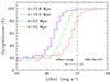 |
Fig. 3. Completeness function in luminosity of the H II regions detected by HIIPHOT for galaxies belonging to the different substructures of the cluster located at 15.8 (cluster B, C; magenta), 16.5 (cluster A, LVC; blue), 23 (W′ cloud; green), and 32 Mpc (W and M clouds; red), respectively. The vertical dashed line shows the limit in Hα luminosity adopted to define a complete sample where statistical properties are derived. The black arrows show how the position of a limiting Hα luminosity L(Hα) = 1037 erg s−1 should be shifted for a dust attenuation of A(Hα) = 1 mag or a [N II] contamination of [N II]/Hα = 0.5 (for reference, the measured values for NGC 4321 used for this test are A(Hα) = 0.85 mag and [N II]/Hα = 0.48). |
3.6. Comparison with the literature
We checked the accuracy of the derived parameters by comparing them to those extracted from an independent set of H II regions extracted from MUSE data gathered during the PHANGS survey of nearby galaxies (Emsellem et al. 2022) and recently published and analysed in Santoro et al. (2022). The two sets of data have three massive galaxies in common, NGC 4254, NGC 4321, and NGC 45356. We recall that the parameters of the H II regions of these galaxies in the PHANGS data have been extracted using a modified version of the HIIPHOT pipeline optimised to work on IFU spectroscopic data. The main differences with the one used on the VESTIGE data are: i) the PHANGS Hα data are corrected for dust attenuation and do not include any [N II] contamination; ii) the PHANGS data are not corrected for the emission line flux of the background, that is the diffuse ionised gas (DIG) component permeating star-forming discs (Haffner et al. 2009). As stressed in Santoro et al. (2022), this diffuse emission becomes relevant only in the fainter H II regions; iii) the PHANGS data cover just a fraction of the disc of all the three targets, where the contribution of the stellar continuum emission and of the DIG are important.
The comparison of the fluxes extracted by HIIPHOT on the two sets of data is shown in Figures 4, 5, and 6. For consistency, the comparison is done using VESTIGE observed fluxes not corrected for the DIG emission. The comparison of the two sets of data shows that a higher number of H II regions is detected in the VESTIGE NB imaging data than in the MUSE/PHANGS IFU spectroscopic data. This is probably due to the fact that a more aggressive surface brightness threshold is adopted in this work compared to the one used on the PHANGS data. Table 2 gives the difference in logarithmic scale between the fluxes in the Hα + [N II] emission line uncorrected for DIG emission and measured between the two instruments. The agreement between the two sets of data is very good (systematic difference of ∼0.10 dex with a dispersion of ∼0.20 dex), and this despite the use of a different HIIPHOT extraction code on a completely different set of data. The difference in the two sets of data is reduced in those H II regions extended over more than 50 pixels (blue symbols), the most extended regions resolved by the two instruments. This result suggests that the seeing can slightly affect the output of the code and stresses once again the importance of using a uniform set of high-quality imaging data for such an analysis. VESTIGE is providing this ideal sample given that all images have been gathered during excellent and very constant seeing conditions (see Fig. 2). Figures 4, 5, and 6 do not show any increase of the systematic difference between the two sets of data in the brightest H II regions, where the contribution of the line emission in the broad-band r filter is expected to be more important, suggesting that this effect is negligible. The available set of data does not allow us to test whether the scatter in the relations is correlated to any other physical parameter such as the metallicity or dust attenuation in the H II region or to the underlying Balmer absorption in the Hα line. Considering that the typical instrumental uncertainty in the MUSE data is of the order of ∼5% (from the instrument documentation), that on the Hα measurement of another ≲2% (Santoro et al. 2022), and that part of the scatter is due to the different apertures identified by HIIPHOT in the IFU MUSE data and in the NB VESTIGE imaging data, we can conclude that the uncertainty in the measured fluxes (≃0.15 dex if we consider that part of the dispersion in the Figures 4, 5, and 6 is due also to the MUSE data) is small compared to the dynamic range of the relations and distributions analysed in this work. We thus expect that the impact of the third-order effects mentioned here and in Sect. 3.3 are negligible in the following analysis. In Appendix A we show how the use of a single correction for dust attenuation and [N II] contamination derived using integrated measurements for each individual galaxy does not have major systematic effects in the derived parameters.
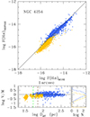 |
Fig. 4. Relationship between the flux of individual H II regions of NGC 4254 extracted from the VESTIGE images and from the MUSE/PHANGS datacubes. For consistency with the MUSE data, the VESTIGE data are the output of HIIPHOT uncorrected for the diffuse emission. The lower panel shows how the ratio of the VESTIGE-to-PHANGS flux ratio changes as a function of the effective diameter corrected for seeing smearing. The vertical green dashed line corresponds to the seeing of the VESTIGE image, the vertical brown dashed line to the seeing of the MUSE/PHANGS dataset. Blue dots (orange circles) are for H II regions with more (less) than 50 pixels in the VESTIGE image (regions with a typical radius of ≃0.75″). The distributions of their ratio is given in the lower right panel. |
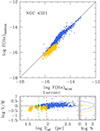 |
Fig. 5. Relationship between the flux of individual H II regions of NGC 4321 extracted from the VESTIGE images and from the MUSE/PHANGS datacubes (see Fig. 4 for details). |
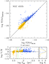 |
Fig. 6. Relationship between the flux of individual H II regions of NGC 4535 extracted from the VESTIGE images and from the MUSE/PHANGS datacubes (see Fig. 4 for details). |
Comparison of VESTIGE versus PHANGS/MUSE.
3.7. Sample of H II regions in the unperturbed sample
Adopting the above criteria, we end up with a sample of 27.330 H II regions in 64 gas-rich (H I−def ≤ 0.4), unperturbed systems. Of these, 13.278 have a Hα luminosity corrected for dust attenuation and [N II] contamination L(Hα) ≥ 1037 erg s−1. This is the final sample of H II regions analysed in this work. Those with an effective diameter derived assuming a correction ≤50% (see Eq. (2)) are 11 293, and 6520 when limited to L(Hα) ≥ 1037 erg s−1. The galaxies analysed in this work (unperturbed sample) are listed in Table B.1 along with their parameters. Table B.2 gives the parameters of the elliptical apertures used for the identification of the H II regions and for the extraction of the total Hα flux. Tables B.1 and B.2 are given in Appendix B.
4. Analysis
In this section we analyse the statistical properties of the H II regions in unperturbed cluster galaxies. We do that first by deriving the composite distribution of the whole unperturbed sample (luminosity function, effective diameter, and electron density distribution) and the luminosity-diameter relation. Composite luminosity functions and distributions are important to derive the statistical properties of a complete sample of H II regions in the Virgo cluster. Although these distributions might marginally change when derived in the different cluster substructures, as they do from galaxy to galaxy, they composite shapes can be used as reference for comparative studies for samples of galaxies located in different environments (voids, field, groups, other clusters etc.). They also provide sufficient statistics to analyse dwarf systems, otherwise impossible for their very limited number of H II regions. We then study the main scaling relations between several representative properties of individual H II regions and those of their parent galaxy. All this analysis is made possible thanks to the excellent statistic, the large dynamic range in the parameter space of galaxies properties, and the uniform quality of the data which minimises any possible bias.
4.1. Composite distributions
4.1.1. Composite luminosity function
Figure 7 shows the composite Hα luminosity function of all the H II regions of the unperturbed sample. The Hα luminosities are corrected for [N II] contamination and dust attenuation as mentioned above. This function is constructed by counting the number of H II regions per bin of Hα luminosity (0.25 dex in log scale; differential luminosity function). The distribution shows a steep rise of the number of H II regions from L(Hα) ≃ 1040.5 erg s−1 to L(Hα) ≃ 1039 − 39.5 erg s−1, a relative flattening up to L(Hα) ≃ 1036.5 erg s−1, with a moderate (up to L(Hα) ≃ 1036 erg s−1) then an abrupt decrease below this luminosity due to completeness (see Sect. 3.5 and Fig. 3).
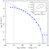 |
Fig. 7. Composite luminosity function of the H II regions detected by HIIPHOT on the selected galaxies. The Hα luminosities of individual H II regions have been corrected for dust attenuation and [N II] contamination as described in Sect. 3.2. The solid and dotted lines indicate the best-fit and 1σ confidence regions for the Schechter luminosity function parametrisation. The vertical dashed line shows the completeness of the survey. The small panel in the top right corner indicates the 1σ probability distribution of the fitted Schechter function parameters. |
Following the same procedure described in Mehta et al. (2015), Fossati et al. (2021), and Boselli et al. (2023b), we tentatively fit the distribution with a Schechter (1976) function of the form of ℒ = log10(L):
 (4)
(4)
with dℒ = dlog10(L), ℒ* = log10L* (in units of erg s−1), where we derived the posterior distribution and the best-fit parameters using the MULTINEST Bayesian algorithm (Feroz & Hobson 2008; Feroz et al. 2019). The terms L*, Φ*, and α are the characteristic luminosity at the knee of the distribution, the number of objects at L*, and the slope of the distribution at the faint end, respectively. We limited the fit of the Schechter function to L(Hα)≥1037 erg s−1, where the sample is almost complete (see Sect. 3.5). The adopted function reproduces the data, although with a systematic underestimate of the number of bright H II regions for L(Hα)≳1040.5 erg s−1, where the statistic is poor, and overestimating it at the faint end (L(Hα)≲1037.5 erg s−1), where incompleteness might start to be present. Despite these systematic differences, a Schechter function is here more indicated than a single or double power law, as often used in the literature (e.g. Kennicutt et al. 1989a; Beckman et al. 2000; Helmboldt et al. 2005; Bradley et al. 2006; Liu et al. 2013; Cook et al. 2016; Santoro et al. 2022), because the data have a smooth distribution, steep at the bright end and flat at the faint end. The parameters of the best fit for individual galaxies are given in Table B.3, while those for the composite luminosity functions in Table 3 (median of the posterior samples from the nested sampling solver, with uncertainties). They are given for the composite luminosity function (first row) or the mean of the parameters with the dispersion of their distribution derived for those galaxies having more than 20 H II regions7 of luminosity L(Hα) ≥ 1037 erg s−1 (27 objects, second row). These are all galaxies with a stellar mass Mstar ≥ 108 M⊙ (see Sect. 4.2.2 and Table B.1). The individual luminosity functions of these 27 galaxies are shown in Fig. E.1. The fitting method used in this work is optimised to treat distributions with different statistical numbers and uncertainties on the sampled range, as is the case for a luminosity function from the faint to the bright end, since it uses individual points rather than binned data (e.g. Mehta et al. 2015). The outputs of the fit might thus systematically differ from those gathered using other fitting techniques as done in previous works. The comparison with other works, however, is made difficult by other factors such as the choice of different parametric functions (e.g. power low versus Schechter function), dust attenuation and [N II] contamination corrections, completeness, or sampled Hα luminosity range. Despite the adopted Schechter function only approximately fits the observed distributions, the homogeneity of the sample in terms of completeness and the use of the same fitting function within the same luminosity range for all targets secures a robust comparative analysis of the output parameters.
Parameters of the Schechter functionss.
Figure 8 shows the normalised luminosity function derived for H II regions located inside or outside the deprojected effective radius measured in the i-band, available to the NGVS team, and measured as described in Ferrarese et al. (2020). The total number of H II regions with L(Hα) ≥ 1037 erg s−1 located outside the effective radius (9084) exceeds by a factor of ∼2 the one located in the inner regions (4194). Despite that, the brightest H II regions are preferentially located in the inner disc, some of which at less than 3 arcsec from the nucleus (12/64), as indicated by the different shape of the two functions (a Kolmogorov-Smirnov test indicates that the two distributions are statistically different, p-value = 1.3 × 10⁻¹⁹). The faint-end slope of the distribution in the inner regions is flatter than the one observed in the outer discs. The difference in the distributions observed below L(Hα)≲1037.5 erg s−1, however, should be considered with caution since it might result form possible biases in the HIIPHOT pipeline in detecting H II regions of low luminosity located in crowded regions, in particular where the stellar continuum might be important (inner disc, see Pleuss et al. 2000; Bradley et al. 2006). Indeed, it is likely that incompleteness, if present, is more important in the inner regions, where crowding is also more important. Finally, to quantify any possible effect related to the different distance of galaxies, we construct and compare four independent composite luminosity functions for galaxies located in the different substructures of the cluster (Fig. 9). Although this test is limited by poor statistics for galaxies located in the W′ (23 Mpc), W and M clouds (32 Mpc), we do not observe any strong dependence of the best-fit parameters with distance, nor a clear sign of incompleteness in the lowest luminosity bins in the distribution for galaxies located in the far W′, W, and M clouds, suggesting that the luminosity function shown in Fig. 7 well represents the distribution of luminosities in unperturbed, gas-rich systems. Figure 10 shows the relation between the faint end slope and the characteristic luminosity measured for all the individual galaxies with more than 20 H II regions of Hα luminosity corrected for dust attenuation and [N II] contamination L(Hα)≥1037 erg−1. The two parameters are not correlated, and no trend with distance is observable.
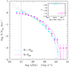 |
Fig. 8. Composite luminosity function of the H II regions detected within (magenta) and outside (cyan) the i-band effective radius of the target galaxies normalised to the total number of H II regions with L(Hα)≥1037 erg s−1 within (Ntot = 4194) and outside (Ntot = 9084) the effective radius. The vertical dashed line shows the completeness of the survey. The small panel in the top right corner indicates the 1σ probability distribution of the fitted Schechter function parameters. |
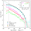 |
Fig. 9. Composite luminosity function of the H II regions detected by HIIPHOT on the selected galaxies. Different colours are used for galaxies belonging to different cluster substructures: cyan for cluster A and LVC, 16.5 Mpc; magenta for cluster B, 15.8 Mpc; green for W′ cloud, 23 Mpc; and red for W and M clouds, 32 Mpc. The Hα luminosities of individual H II regions are corrected for dust attenuation and [N II] contamination as described in Sect. 3.2. The solid and dotted lines indicate the best-fit and 1σ confidence regions for the Schechter luminosity function parametrisation. The vertical dashed line shows the completeness of the survey. The small panel in the top right corner indicates the 1σ probability distribution of the fitted Schechter function parameters. |
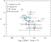 |
Fig. 10. Relation between the faint end slope α of the luminosity function and the characteristic luminosity of individual galaxies with more than 20 H II regions brighter than L(Hα)≥1037 erg s−1. Different colours are used for galaxies belonging to different cluster substructures: cyan for cluster A and LVC, 16.5 Mpc; magenta for cluster B, 15.8 Mpc; green for W′ cloud, 23 Mpc; and red for W and M clouds, 32 Mpc. The Hα luminosities of individual H II regions are corrected for dust attenuation and [N II] contamination as described in Sect. 3.2. |
4.1.2. Composite diameter distribution
Figure 11 shows the combined distribution of the observed and corrected for the seeing (6520 regions) equivalent diameters of H II regions with an Hα luminosity L(Hα)≥1037 erg s−1. The distribution shows a constant increase from Deq ≃ 600 to 100 pc with a steep decrease below this limit. The difference between the observed and corrected for seeing effects distributions becomes significant below Deq ≲ 100 pc, with an expected lower number of corrected measurements when the sample includes only moderately corrected values (Deq/DHII ≥ 0.5). Figure 12 shows the distribution of the equivalent diameters corrected for seeing effects for H II regions of luminosity L(Hα)≥1037 erg s−1 located within (1834 objects) and outside (4686) the i-band effective radius of the galaxy. A Kolmogorov-Smirnov test indicates that the two distributions are statistically different (p-value = 3.7 × 10⁻⁵). We observe a mild excess of extended regions in the inner galaxy discs than in the outer regions. These differences, as the observed difference at small diameters (Deq ≲ 100 pc) might be related to confusion and incompleteness more important in the crowded inner regions of the stellar disc. As for the luminosity function, we do not observe any evident variation of the equivalent diameter distribution with the distance of galaxies (Fig. 13).
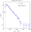 |
Fig. 11. Distribution of the observed (black dots) and corrected for seeing effects (blue dots) equivalent diameters for H II regions with L(Hα)≥1037 erg s−1. The dashed vertical line shows the equivalent diameter corresponding to the mean seeing of the survey at the distance of the cluster (16.5 Mpc). |
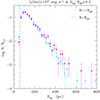 |
Fig. 12. Normalised distributions of the equivalent diameters corrected for seeing effects measured within (magenta) and outside (cyan) the i-band effective radius of the selected galaxies for H II regions with L(Hα)≥1037 erg s−1. The dashed vertical line shows the equivalent diameter corresponding to the mean seeing of the survey at the distance of the cluster (16.5 Mpc). |
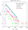 |
Fig. 13. Distribution of the equivalent diameters corrected for seeing effects equivalent diameters for H II regions with L(Hα)≥1037 erg s−1. The different colours are for galaxies belonging to different cluster substructures: cyan for cluster A and LVC, 16.5 Mpc; magenta for cluster B, 15.8 Mpc; green for W′ cloud, 23 Mpc; and red for W and M clouds, 32 Mpc. The dashed vertical lines show the equivalent diameter corresponding to the mean seeing of the survey at the distance of the different cluster substructures. |
4.1.3. Composite electron density distribution
Figure 14 shows the distribution of the electron density derived using Eq. (3) for H II regions with L(Hα) ≥ 1037 erg s−1 and equivalent diameters corrected for seeing effects with corrections not exceeding 50%. The distribution is peaked at ne ≃ 2 cm−3, and sharply decreases up to ne ≃ 7–8 cm−3, where it reaches its minimum. There are a very few regions with densities ne > 8 cm−3. Figure 15 shows the same distribution derived for H II regions located within and outside the i-band effective radius of the parent galaxies. Although the two distributions look very similar, a Kolmogorov-Smirnov test indicates that they are drown by statistically different populations (p-value = 10−7). Again, we do not observe any clear dependence of the shape of the composite electron density distribution with the distance of galaxies located in the different cluster substructures (Fig. 16). We notice, however, that the distributions of ne look steeper in cluster B and W′ than in the W and M clouds or in cluster A and LVC. We also notice that in the different subclusters the distributions are very noisy even at their peak where the statistic is sufficiently high, while the comparison at ne ≳ 4 cm−3 is impossible given the very limited number of H II regions.
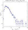 |
Fig. 14. Distribution of the electron density derived using equivalent diameters corrected for seeing effects for H II regions with L(Hα)≥1037 erg s−1 and a diameter correction factor ≤50%. |
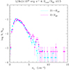 |
Fig. 15. Normalised distributions of the electron density derived using equivalent diameters corrected for seeing effects for H II regions with L(Hα)≥1037 erg s−1 for H II regions located inside (magenta) and outside (cyan) the i-band effective radius. The two distributions are normalised to the total number of regions located within and outside the effective radius. The number of H II regions with densities ne ≥ 7.5 cm−3 for the two samples are most one per bin but are plotted at different positions because of the different normalisation. |
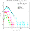 |
Fig. 16. Distribution of the electron density derived using equivalent diameters corrected for seeing effects for H II regions with L(Hα)≥1037 erg s−1 and a diameter correction factor ≤50%. Different colours are for galaxies belonging to the different Virgo cluster substructures (cyan for cluster A and LVC, 16.5 Mpc; magenta for cluster B, 15.8 Mpc; green for W′ cloud, 23 Mpc; red for W and M clouds, 32 Mpc). |
4.1.4. Luminosity-diameter relation
Figure 17 shows the relation between Hα luminosity of individual H II regions corrected for [N II] contamination and dust attenuation and the equivalent diameter corrected for seeing effects. The two variables are tightly correlated, with the Hα luminosity of the individual H II regions increasing with the size. Figure 18 shows the same relation for H II regions located within and outside the i-band effective radius of the parent galaxy. The best-fit parameters are given in Table 4. The relation is flatter when no limits on the diameter correction are applied. The difference between the two relations in the inner and outer disc regions seems statistically significant, with a steeper slope observed in the inner regions, although the two best fits are within the 1σ dispersion of the two distributions. The slope of the relations is fairly constant while the intercepts slightly change when measured on the subsample of galaxies located at different distances (Fig. 19). The decrease of the intercept with increasing distance observed between cluster A + LVC, W′, and W + M is expected given the slope of the relation (≃3.4–3.5) and that at further distances only the largest H II regions are resolved, thus reducing the dynamic range of the relation. This, however, does not explain the observed difference between cluster A + LVC and cluster B. We recall, however, that the difference between the two intercepts is just marginal (∼2 sigma), as the difference in distance of the two subclusters A and B (0.7 Mpc) as measured by Cantiello et al. (2024) using mainly early-type galaxies. The distance of the star-forming systems hosting the H II regions analysed in this work might not exactly match that of early-types since most of them are now infalling for the first time into the cluster (e.g. Gavazzi et al. 1999). Any interpretation of the observed difference in the intercept of the L(Hα) versus Deq relation between cluster A and B in terms of distance of galaxies should thus be done with extreme caution.
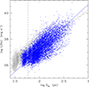 |
Fig. 17. Relation between the Hα luminosity of individual H II regions corrected for [N II] contamination and dust attenuation and the equivalent diameter corrected for seeing effects. Blue filled dots are for H II regions with a diameter correction factor ≤50%, grey dots for all H II regions with no limits in diameter correction. The vertical dashed line shows the mean FWHM of the survey assuming galaxies at the distance of the main body of the cluster (16.5 Mpc). The blue solid line gives the bisector fit (Isobe et al. 1990) of the relation derived for H II regions with a diameter correction factor ≤50% (blue dots), the grey solid line for H II regions with no limits in the diameter correction. |
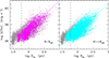 |
Fig. 18. Relation between the Hα luminosity of individual H II regions corrected for [N II] contamination and dust attenuation and the equivalent diameter corrected for seeing effects for regions located within (right, filled magenta dots) and outside (left, filled cyan dots) the i-band effective radius of the parent galaxy, where the correction is less than 50%. Grey dots show all H II regions with no limits in luminosity and diameter correction. The vertical dashed line shows the mean FWHM of the survey assuming galaxies at the distance of the main body of the cluster (16.5 Mpc). The magenta and cyan solid lines give the bisector fit of the relations derived for galaxies with a diameter correction factor ≤50% (magenta and cyan filled dots). |
Best-fit parameters for the luminosity-size relation (log L(Hα) = a × log Deq + b).
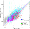 |
Fig. 19. Relation between the Hα luminosity of individual H II regions corrected for [N II] contamination and dust attenuation and the equivalent diameter corrected for seeing effects. Coloured (cyan for cluster A and LVC, 16.5 Mpc; magenta for cluster B, 15.8 Mpc; green for W′ cloud, 23 Mpc; red for W and M clouds, 32 Mpc) dots are for H II regions with a diameter correction factor ≤50%, and the grey dots are for all H II regions with no limits in diameter correction. The vertical dashed lines show the mean FWHM of the survey assuming for the different substructures of the cluster. The coloured solid lines give the bisector fit of the relation derived for galaxies with a diameter correction factor ≤50%. |
4.2. Scaling relations
We analyse in this section the main scaling relations between several representative properties of the H II regions and the main properties of their parent galaxies for a statistically significant sample of unperturbed systems spanning a wide range in stellar mass and morphological type. Hα luminosities are corrected for [N II] contamination and dust extinction as indicated in Sect. 3.2.
Figure 20 shows the relation between the total number of H II regions with L(Hα)≥1037 erg s−1 and the total star formation rate (upper left panel), stellar mass (lower left), mean star formation rate (upper right) and stellar mass density (lower right) within the i-band effective radius of the parent galaxies. As expected, the number of H II regions linearly increases with the total star formation rate and the stellar mass since “bigger galaxies have more of everything” (Kennicutt 1990). The parameters of the best fit of Fig. 20 and of the following Figs. C.1–C.6 are shown in the Figures and given in Table 5 only whenever the probability P that the two variables are correlated with P ≥ 95% (p-value < 0.05). All the following figures relative to the scaling relations discussed in this and in the next sections are given in Appendix C.
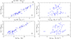 |
Fig. 20. Relation between the total number of H II regions detected by HIIPHOT with L(Hα)≥1037 erg s−1 and the total star formation rate (upper left panel), total stellar mass (lower left), mean star formation rate surface density (upper right), and mean stellar mass surface density (lower right) of the host galaxies. Star formation rates (lower axis) have been derived from Hα luminosities (upper axis) corrected for dust attenuation and [N II] contamination assuming a Chabrier IMF. The black dashed line shows the best fit to the data (bisector fit). The dot in the lower right corner shows the typical error bar in the data. |
We observed a scattered diagram whenever the total number of H II regions with L(Hα) ≥ 1037 erg s−1 was plotted versus the logarithm of the star formation and of the stellar mass surface densities, where these two normalised entities are defined as the mean star formation rate and stellar mass within the deprojected effective radius Reff, here measured in the i-band (radius containing 50% of the i-band light) as described in Ferrarese et al. (2020, and available to the NGVS team; see Fig. 20):
![Mathematical equation: $$ \begin{aligned} {\mu _{\rm SFR} = \frac{\mathrm{SFR}}{2 \pi R_{\rm eff}^2} \,\mathrm {[M_{\odot } \,yr^{-1}\,kpc^{-2}]}} \end{aligned} $$](/articles/aa/full_html/2025/04/aa50963-24/aa50963-24-eq6.gif) (5)
(5)
and
![Mathematical equation: $$ \begin{aligned} {\mu _{\rm star} = \frac{M_{\rm star}}{2 \pi R_{\rm eff}^2} \, \mathrm {[M_{\odot }\,kpc^{-2}]}}. \end{aligned} $$](/articles/aa/full_html/2025/04/aa50963-24/aa50963-24-eq7.gif) (6)
(6)
We stress that the mean surface densities defined in Eqs. (5) and (6) uses i-band effective radii and not radii measured on the Hα and stellar mass 2D distributions. While the i-band distribution well traces that of stellar mass, this is not necessary the case for the distribution of star-forming regions. Indeed, Equation (5) is an hybrid definition roughly measuring the star formation activity normalised to the size of the stellar disc as defined by the old stellar population, and should thus be considered with caution. We adopted this hybrid definition since more indicated than the standard mean star formation rate surface density definition (star formation rate divided by the size of the star-forming disc measured in Hα) to quantify the truncation of the star-forming disc with respect to that of the stellar disc occurring in ram pressure stripped galaxies (Boselli et al. 2022b), something which will be fully analysed in a future VESTIGE paper.
Figure C.1 shows the relations between the Hα luminosity of the brightest H II region and the total star formation rate, stellar mass (and their surface densities) of the parent galaxies. The same figures done using the mean luminosity of the first three ranked H II regions and the same galaxy parameters are also shown in Appendix C. The Hα luminosity of the brightest H II region is tightly related to the star formation rate, stellar mass, mean star formation rate and stellar mass surface density of their host. The brightest H II regions with luminosities L(Hα) ≃ 1040 erg s−1 are preferentially located in those systems with the highest star formation rate.
Figure C.2 shows the relation between L(Hα)≥37/L(Hα), defined as the ratio between the sum of the Hα luminosity of all the H II regions with luminosity L(Hα) ≥ 1037 erg s−1 and the integrated Hα luminosity of the galaxy, and the total star formation rate, the total stellar mass and their surface densities of the host galaxies. The ratio L(Hα)≥37/L(Hα) roughly corresponds to the fraction of Hα emission due to compact H II regions, and is thus a direct estimate of the DIG in these normal, star-forming systems. This ratio is always in the range −0.7≲ log L(Hα)≥37/L(Hα) ≲ 0 and does not changes with stellar mass and star formation rate, but rather increases with increasing star formation rate and stellar mass mean surface densities, suggesting that the contribution of the DIG increases in those galaxies where the density of stars is low (i.e. low surface brightness systems), which are also objects where the star formation rate surface density is low given that the two variables are also correlated (see Appendix D).
Figure C.3 shows the dependence of the ratio on three different parameters characterising the physical properties of the ISM where stars are formed: the metallicity of the gas, the fraction of molecular-to-atomic gas, and the total gas-to-dust ratio. With the only exception of the metallicity, which is available for 39/64 galaxies of the unperturbed sample, the two other parameters are limited to the most massive galaxies where both the molecular gas (CO) and dust masses are measured. This limits the sampled parameter space. Figure C.3 shows that the L(Hα)≥37/L(Hα) ratio is fairly constant in galaxies having a molecular-to-atomic gas ratio in the range 0.03 ≲ MH2/MHI ≲ 1.6 and a total gas-to-dust ratio 100 ≲ G/D ≲ 650. On the contrary, the ratio decreases with increasing metallicity, from L(Hα)≥37/L(Hα) ≃ 0.9 at 12 + log O/H ≃ 8.1 to L(Hα)≥37/L(Hα) ≃ 0.4 at 12 + log O/H ≃ 8.7.
Figure C.4 shows the relation between L(Hα)1/L(Hα), the ratio between the luminosity of the brightest H II region and the total Hα luminosity of the galaxy, and the integrated star formation rate and stellar mass of the host. We recall that out of the 66 galaxies with H I−def≤ 0.4, only two have L(Hα)1< 1037 erg s−1 and are thus excluded from the unperturbed sample. As defined, the sample is thus not biased to those galaxies with bright H II regions. Similar figures with the contribution of the brightest three H II regions to the total Hα luminosity of the galaxy are shown in Appendix C. Figure C.4 indicates that the contribution of the brightest H II regions to the total Hα emission of galaxies strongly increases from ≃1–10% in star-forming (SFR ≃ 1 M⊙ yr−1) and massive (Mstar ≃ 1010 M⊙) objects to ≃50–100% in dwarf systems (SFR ≃ 10−3 M⊙ yr−1; Mstar ≃ 107 M⊙).
Figure C.5 shows the relation L(Hα)1/L(Hα) and the metallicity, the molecular-to-atomic gas ratio, and the total gas-to-dust ratio. The poor statistic (15 objects) prevents us to see whether L(Hα)1/L(Hα) is related to MH2/MHI and Mgas/Mdust, but Fig. C.5 clearly shows an anti-correlation with the gas metallicity.
Figure C.6 shows the relation between the ratio of the total Hα luminosity of H II regions with L(Hα) ≥ 1037 erg s−1 (L(Hα)≥37/L(Hα)), of the brightest H II region (L(Hα)1/L(Hα)), and of the sum of the Hα luminosity of the brightest three H II regions (L(Hα)3/L(Hα), measured only for those galaxies with at least 3 H II regions with L(Hα) ≥ 1037 erg s−1, where L(Hα)3 is the contribution of the three brightest H II regions) and the integrated Hα luminosity and the specific star formation rate of the parent galaxies (SSFR). The three variables are only marginally related to the specific star formation rate. While at low specific star formation rates (log SSFR ≲ −10.5 yr−1) all ratios with −0.7 ≲ log L(Hα)≥37/L(Hα) ≲ 0, −2≲ log L(Hα)1/L(Hα)≲ 0, and −1.6≲ log L(Hα)3/L(Hα) ≲ 0 are observed, in those systems with the highest specific star formation rate only the highest ratios are present, suggesting that only in these extreme systems the contribution of all the individual H II regions, or that of the brightest ones, to the total ionising radiation of galaxies is dominant.
4.2.1. Relations with morphological type
We checked whether the main normalised properties of H II regions change in different morphological classes, as previously stated in the literature (e.g. Kennicutt et al. 1989a, see Fig. C.7). We do not observe any clear variation of the density of H II regions of luminosity L(Hα) ≥ 1037 erg s−1 per unit disc size with morphological type, where the size of the galaxy is measured using the optical diameter at the 25.5 isophote (extracted from Binggeli et al. 1985 whenever available or derived from the g-band NGVS effective radius using a relation previously calibrated on objects with both measurements available). The only exception are BCD galaxies where the density of H II regions is increased with respect to that observed in the other morphological classes. We also do not observe any variation of the number of H II regions of luminosity L(Hα) ≥ 1037 erg s−1 per unit stellar mass with the morphological type.
4.2.2. Fit parameters of the luminosity function on individual galaxies
We fitted the Hα luminosity function of H II regions in individual galaxies using the same parametric Schechter (1976) function given in Eq. (4). Because the observed shape of the non-parametric luminosity function abruptly decreases below L(Hα) ≲ 1037 erg s−1 (see Sect. 3.5), we limited the fit to H II regions of luminosity L(Hα) ≥ 1037 erg s−1. We also limited the fit to those objects with at least 20 H II regions detected above this luminosity limit (27 objects, all with Mstar ≳ 108 M⊙). Figures C.8–C.10 show how the fitted characteristic parameters α, L*, and Φ* are related to the total star formation rate, stellar mass, mean star formation rate and stellar mass surface brightness. The best-fit parameters of the Schechter function are given in Table B.3, while the fitted functions are compared to the data in Fig. E.1.
Figure C.8 shows that slope of the faint end of the luminosity function is only barely related to the total star formation rate of the host but not to their total stellar mass. On the contrary, the slope α is tightly related to the mean star formation and stellar mass surface densities of their host galaxies. Objects with a high surface density of star-forming regions or evolved stars have, on average, a flatter slope of the Hα luminosity function of H II regions at the faint end than those characterised by low densities of recently formed or evolved stars. On the contrary, the characteristic luminosity L* is not related to the star formation rate, stellar mass, and their mean surface densities (Fig. C.9). The characteristic parameter Φ*, which gives the number of H II regions at L*(Hα), is related, although with a significant dispersion, to the total star formation rate, stellar mass, and mean star formation rate and stellar mass surface density of the host galaxies (Fig. C.10). The relation with the stellar mass and the star formation rate is expected being Φ* a scale parameter counting the number of H II regions in each object. Out of these three parameters, only α is barely related to the specific star formation rate of the host galaxies (Fig. C.11). We also investigated the relationship between α, L*, and Φ*, and three parameters characterising the properties of the ISM, metallicity, molecular-to-atomic, and total gas-to-dust ratio, but we did not found any clear relation.
4.3. Radial variations
We also study the variation of the properties of H II regions with their deprojected radial distance from the galaxy centre. For this purpose, we divide H II regions located inside and outside the effective radius measured in the i-band. We do not observe any relation between the ratio of number of H II regions with luminosity L(Hα) ≥ 1037 erg s−1 located within and outside the i-band effective radius and the morphological type, star formation rate, and stellar mass (and their associated surface densities) of the host galaxies. The ratio distribution has a mean value of log  , corresponding to
  .
.
5. Discussion
The main purpose of this work is that of providing a reference for future studies. Most of the relations analysed in this work have been already studied in dedicated papers. Their physical interpretation has been extensively discussed in these works, to which we address the interested readers. Here we will briefly discuss the main results of this analysis in comparison with what already presented in the literature.
5.1. Strengths and weaknesses of the sample
The statistical analysis presented in this work is based on a sample of 64 unperturbed star-forming galaxies with 13 278 H II regions of luminosity L(Hα) ≥ 1037 erg s−1 located at the periphery of the Virgo cluster. Despite this large statistic, the data used in this work have several limitations which should be considered in the discussion. First of all, the Hα luminosities of individual H II regions are corrected for [N II] contamination and dust attenuation using a single value which changes from galaxy to galaxy. This is not the case in similar studies based on samples of H II regions observed with IFU spectroscopy such as those recently conducted or under way using VLT/MUSE (PHANGS, Santoro et al. 2022; Groves et al. 2023, MAUVE), CFHT/SITELLE (SIGNALS, Rousseau-Nepton et al. 2018, 2019), or Calar Alto/PPAK (CALIFA, Sánchez et al. 2015; Espinosa-Ponce et al. 2020). IFU spectroscopy allows for an accurate determination of [N II] contamination and dust attenuation in each individual H II region. IFU data are thus more suitable to trace variations within the disc of galaxies, where metallicity and dust attenuation gradients are present.
Our set of data, however, has several other advantages. First of all, it is composed of galaxies located all at almost the same distance with a unique set of data all of similar quality in terms of sensitivity and angular resolution. It includes objects spanning a wide range in morphological type (from lenticulars to spirals, Magellanic irregulars and BCDs) and stellar mass (107 ≲ Mstar ≲ 1011 M⊙). It is thus ideally suited to study scaling relations and to become a reference for future comparative analyses. We recall that, at this sensitivity, the data allow us to detect a single early-B ionising star (L(Hα) ≃ 1036 erg s−1) if located in uncrowded regions, and to resolve H II regions of diameter ≳60 pc. Up to now, these low luminosities have been reached on statistically significant samples only in a handful of galaxies belonging to the Local Group (e.g. Kennicutt et al. 1989a,b), or using 8 metre class telescopes on nearby samples of massive galaxies (Mstar ≳ 109.5 M⊙, Santoro et al. 2022). Other statistical samples are generally limited in terms of sensitivity and angular resolution (Caldwell et al. 1991; Banfi et al. 1993; Rozas et al. 1996a; Elmegreen & Salzer 1999; Thilker et al. 2002; Helmboldt et al. 2005; Bradley et al. 2006). Furthermore, our sample includes galaxies located in a nearby cluster, and is thus suitable to study the effects of the environment on galaxy evolution down to the scale of individual H II regions. This will be the topic of a forthcoming publication.
5.2. Parameters of the luminosity function
The data in our hand allow us to trace the statistical properties of this representative set of local galaxies. The composite Hα luminosity function of individual H II regions can be fitted with a Schechter function of faint end slope α = −1.61 ± 0.01 and characteristic luminosity L*(Hα) = 39.68 ± 0.04 erg s−1. When fitted to individual galaxies having more than 20 H II regions above the threshold of L(Hα)≥1037 erg s−1, ⟨α⟩= − 1.66, with a dispersion σ = 0.43, where ⟨α⟩ is the mean slope derived on a sample of 27 objects. We recall that the fit parameters might suffer for low-number statistics in some low-mass objects. Schechter functions are not often used in the literature since data with the sensitivity and angular resolution comparable to those available in this work, necessary to sample a sufficient range in luminosity, are rarely available. Power laws, or double power laws, are generally used. The slope of the power law can be compared to the faint end slope of the Schechter function derived in this work (however, see Sect. 4.1.1). The value derived for the PHANGS sample composed of 19 nearby mostly massive galaxies (Mstar ≳ 109.4 M⊙, Santoro et al. 2022) is ⟨α⟩= − 1.79, with a dispersion σ = 0.15. These parameters have been derived after fitting a power law above a limiting luminosity changing from galaxy to galaxy, with values close to the lower limit used in our analysis (L(Hα)≥1037 erg s−1). The two sets of data give consistent results despite the two samples cover a different range in galaxy stellar mass. This can be explained considering that the α parameter does not depend on the stellar mass of the host galaxies (see Sect. 4.2.2). The values given by Santoro et al. (2022) have been derived using Hα luminosity of H II regions individually corrected for [N II] contamination and dust attenuation. These authors have shown that the use of data uncorrected for dust extinction might induce a slight steepening of the slope. Our set of data might suffer from this effect since the dust extinction correction that we have used is just a rigid shift in the Hα luminosity of all the H II regions belonging to a galaxy. The difference observed at the bright end, where we see a drop of the number of H II regions while Santoro et al. (2022) do not, is possibly partly related to the fact that we include the nuclear region, while they do not. Figure 8 clearly shows that the brightest regions with L(Hα)≥1040 erg s−1 are all located within the effective radius of the galaxies, with 12/64 within 3 arcsec from the nucleus. Given the tight relation between the luminosity of the brightest region L(Hα)1 and the total Hα luminosity of the host galaxy, in ∼20% of the objects the bright end of the luminosity function is dominated by nuclear regions. The faint-end slope of the fitted function found in this work is also consistent with those found in Local Group galaxies by Kennicutt et al. (1989a, α = −2.0 ± 0.5) in a fairly similar luminosity range using uncorrected data, or slightly steeper than those found in another sample of 12 nearby galaxies derived using the Paα line at 1.8756 μm observed with NICMOS/HST (α ≃ −1.0; Liu et al. 2013). It is comparable to that derived for star-forming complexes in the UV band (α ≃ −1.75, Cook et al. 2016) and flatter than the luminosity function of the star clusters populations of nearby galaxies (α = −2.37 ± 0.18, Whitmore et al. 2014, see also Larsen 2002).
A flattening of the distribution below L(Hα)≃1038.6 erg s−1, has been already claimed in the past (e.g. Kennicutt et al. 1989a; Beckman et al. 2000; Bradley et al. 2006). A break at this luminosity has been interpreted in the literature as due to the transition of H II regions from ionisation bounding (the central star or star cluster only ionises the gas within the H II region) at low luminosities to density bounding (a large amount of Lyman continuum photons from the central ionising source escapes the H II region and ionises the diffuse surrounding medium) at higher luminosities (Beckman et al. 2000, see also Lee et al. 2011). The shape of the luminosity function has been also simulated adopting a stellar mass distribution as predicted by an initial mass function and different star formation scenarios (Oey & Clarke 1998). The composite luminosity function derived in this work does not have any sharp discontinuity at the observed break luminosity of L(Hα)≃1038.6 erg s−1, but rather a smooth flattening towards low luminosities characterised by a log L*(Hα) = 39.68 ± 0.04 erg s−1 in the Schechter parametrisation. A sharp discontinuity is also lacking in the luminosity functions of individual galaxies, in particular in the most massive objects unaffected by low-number statistics. Our result is consistent with what derived from the analysis of the PHANGS data, which do not show any evident change of slope at these luminosities. Since a further flattening of the luminosity distribution is seen in our data and in the PHANGS data at L(Hα)≃1037 erg s−1, which corresponds to the completeness limit of the survey, it is conceivable that the Hα luminosity break at L(Hα)≃1038.6 erg s−1 observed in previous works could be due to blending effects in low angular resolution data, as first claimed by Lee et al. (2011).
5.3. Equivalent diameter and electron density distributions
The size distribution of individual H II regions observed in a few well resolved nearby spiral galaxies is generally represented by a power law in the range 50 ≲ log D ≲ 250 pc (Lee et al. 2011; Liu et al. 2013), with the number of regions dropping for smaller size diameters. The limiting diameter at small sizes depends on the linear resolution of the data. The composite distribution observed in our data shows a somewhat different shape (see Fig. 11, as observed in some other objects; Gutiérrez et al. 2011; Liu et al. 2013; Rousseau-Nepton et al. 2018). This gradual variation is visible for Deq ≳ 100 pc, where the correction for seeing effects are negligible. Interestingly, the size composite distribution is very similar to the one observed in NGC 628 by Rousseau-Nepton et al. (2018), although with a slightly different slope. However, a distribution more similar to a power law was observed in our data in the equivalent diameter range 60 ≲ Deq ≲ 300 pc when the brightest galaxies are considered individually. It is thus likely that the observed composite diameter distribution might result from the combination of data for galaxies of different mass and luminosity. Indeed, the scaling relations shown in Sect. 4.2, combined with the luminosity-size relation (Sect. 4.1.2), consistently suggest that galaxies of different mass host regions of different luminosity and size, and thus might populate different regions in the composite equivalent diameter distribution.
The composite electron density distribution is regularly decreasing in the range 2 ≲ ne ≲ 7 cm−3, it has a few objects above this threshold, while it sharply drops at lower densities. A similar distribution is also observed individually in the most massive galaxies where the statistic is sufficiently high. In other galaxies the distribution is fairly symmetric and peaked at a given density (e.g. Liu et al. 2013), with slightly higher values (3 ≲ ne ≲ 30 cm−3, Liu et al. 2013). We note that the range of electron densities derived using NB imaging data (ne ≲ 30 cm−3) is generally lower than the one that can be probed with optical emission lines ([S II] λ6716/6731 Å and [O II] λ3726/3729 Å line ratios; e.g., Kennicutt et al. 1989b) since these indicators are degenerate at these low-density levels (e.g. Osterbrock & Ferland 2006). As extensively discussed in Cedrés et al. (2013), the higher densities given by emission line diagnostics than those measured assuming Eq. (3) are due to the fact that the ionised gas is not uniformly distributed within the H II regions, and the line emission is dominated by the densest inner regions while the equivalent diameter measures the extension of the low-density ionised gas. The observed differences with other works might depend on several factors. First of all, the shape of the distribution and its mean value change according to the adopted [N II] and dust attenuation correction. This is due to the fact that the slope of the luminosity-size relation is not three (see Table 4). Being the electron density defined as a ratio of these two variables (see Eq. (3)), the rigid corrections here applied to the luminosity has thus systematic effects on ne. Furthermore, the absolute values of ne strongly depend on the definition of equivalent diameter and on the adopted corrections for seeing effects. These might change in different works, where the codes used to identify H II regions might change, as the definition of the diameter might also change. Finally, as discussed in the next section, the luminosity-size relation is also strongly affected by observational biases. The comparison with other samples should thus be considered with these caveats whenever these parameters are derived using non-homogeneous sets of data or different tracers.
5.4. Luminosity-size relation
A luminosity-size relation in H II regions in local galaxies has been already observed in the past (e.g. Rozas et al. 1996b; Liu et al. 2013). Liu et al. (2013) reported a slope for the relation of ∼2.5–3 when luminosities are derived using the Paα emission line. Rozas et al. (1996b) finds a slope ∼3 using Hα data. These slopes are consistent with the one found in this work for the composite relation (a = 3.43 ± 0.02). A slope of ∼3 suggests that the luminosity increases linearly with the volume of the region. Scoville et al. (2001) argued that a slope of ∼3 is expected if all H II regions are resolved, while the slope should be closer to ∼2 if blending is important. Figure 17 and Table 4 show a flattening of the relation if all H II regions, including those with a high uncertainty on the adopted correction, are considered. Liu et al. (2013), however, questioned the idea that the flattening of the relation is due to blending with convincing arguments and rather predicted an opposite effect (steepening of the relation with increasing blending). They have shown that the slope of the relation and its scatter depend on the algorithm used to identify and measure the parameters of individual H II regions and on the noise in the data (an increasing noise decreases the slope of the relation). It is thus clear that the slope of the relation is not only related to the intrinsic physical properties of the H II regions but also strongly depends on the quality of the data and on the code adopted for their identification (e.g. Scoville et al. 2001; Liu et al. 2013).
5.5. Scaling relations
5.5.1. General trends
Variations of some representative properties of the H II regions with the properties of their host galaxies (morphological type, luminosity, …) have been already explored in the past (Kennicutt 1988; Kennicutt et al. 1989a; Banfi et al. 1993; Rozas et al. 1996b; Elmegreen & Salzer 1999; Helmboldt et al. 2005; Santoro et al. 2022). Most of the results previously found in the literature are reproduced on strong statistical basis with our dataset. These include the relation between the luminosity of the first ranked H II region (Kennicutt 1988), the shape of the luminosity function (Liu et al. 2013) with several other characteristic parameters of the host galaxies (Santoro et al. 2022). In particular, we find strong dependences of the total number of H II regions (Fig. 20), of the first ranked (Fig. C.1) and of the three first ranked (Fig. C.12) H II regions, with the total Hα luminosity (or star formation rate) and stellar mass of the host galaxies.
The first of these relations is due to a simple scaling factor (bigger galaxies have more of everything). Those relative to the first ranked H II regions can also be understood when combined to the luminosity function. For statistical reasons, the bright end of the luminosity function is populated only in galaxies hosting many H II regions, thus in massive systems with a very strong star formation activity8. They also reflect what found for the massive young star clusters observed with HST in a few nearby galaxies, where the properties of the most massive one is tightly related to the star formation rate density over the galaxy disc (e.g. Larsen 2002; Johnson et al. 2017). Twelve over sixty-four of these bright H II regions are located in the galaxy nucleus. Interesting to note is that the luminosity of the brightest H II regions of some well known galaxies of the Local Group, 30 Doradus (log L(Hα) = 39.76 erg s−1, Kennicutt et al. 1995) in the Large Magellanic Cloud9 (log L(Hα) = 40.49 erg s−1, Kennicutt et al. 2008) and NGC 604 (log L(Hα) = 39.63 erg s−1, Relaño & Kennicutt 2009) in M33 (log L(Hα) = 40.51 erg s−1, Kennicutt et al. 2008) also fall on the upper envelope of the relation shown in Figs. C.1 and C.4.
The observed decrease of the L(Hα)1/L(Hα) ratio with L(Hα) (Fig. C.4) is also expected given that the L(Hα) variable is present on both axis. It is interesting, however, to see that the correlation of L(Hα)1/L(Hα) with Mstar is stronger than with L(Hα), suggesting once again that stellar mass is a fundamental parameter in regulating the star formation process (e.g. Boselli et al. 2001) and thus in driving galaxy evolution (e.g. Cowie et al. 1996; Gavazzi et al. 1996). The relation of L(Hα)1/L(Hα) with metallicity (Fig. C.5) can be easily understood considering that L(Hα)1/L(Hα) is also related to stellar mass (Fig. C.4), as does the gas metallicity (metallicity-mass relation, Tremonti et al. 2004). The fact that the correlation is tighter (higher correlation coefficient, lower dispersion; see Table 5) in the relation with metallicity than with stellar mass (this is also the case when the correlation with Mstar is measured only on the 39/64 galaxies with available metallicity measurements) lets us think that metallicity might participate in regulating the star formation process. This is also suggested by the fact that L(Hα)≥37/L(Hα) is correlated with metallicity (Fig. C.3) while not with stellar mass (Fig. C.2). Metallicity must thus be an important parameter regulating the star formation activity at the scale of individual H II regions.
These well-defined scaling relations can be used to predict the expected number of H II regions in typical unperturbed galaxies in the local Universe undergoing a secular evolution. We do not confirm, however, the observed trends of the number density of H II regions per unit stellar surface and stellar luminosity with morphological type claimed by Kennicutt et al. (1989a).
Interesting is the dependence of several representative parameters (total number of H II regions, luminosity of the first ranked H II regions) with the star formation rate and stellar mass surface density. Dependencies with the surface brightness of the host galaxies have been already noticed by Helmboldt et al. (2005, 2009) and more recently by Santoro et al. (2022) in massive systems. These results have been interpreted as due to a different star formation mode in low-density regimes, where star formation is episodic and with a low efficiency (e.g. Boissier et al. 2008) while it is constant in high surface brightness regions where it generally occurs within spiral density waves (Helmboldt et al. 2005). It is important to remember that the two variables mean star formation and stellar mass surface densities are tightly related (see Appendix D). Although part of this trend might be due to the use of the same normaliser for the two variables, this tight relation is suggesting that the star formation process is triggered by the midplane pressure produced by the stellar gravity of the disc (Shi et al. 2018). The scaling relations on the properties of H II regions shown in Sect. 4.2 thus reflect the general star formation mode observed at the scale of galactic discs. The relation with the specific star formation rate (Fig. C.6) is also very interesting since it indicates that in those systems with the highest present-to-mean past activity the star formation is dominated by one or a few bright H II regions. These are principally BCD galaxies, which can be considered as analogues of starburst at high redshift.
Another interesting result is that the first ranked H II regions (the brightest or the three brightest ones) dominate the total Hα emission of dwarfs. This result is very important since it implies that in these low-mass systems the activity of star formation is dominated by one or a few H II regions. It cannot thus be considered constant over time. We recall that the stationarity condition of the star formation activity on scales as long as the mean age of the emitting stars is a fundamental prerequisite to transform Hα or UV luminosities into star formation rates using the simple prescriptions proposed in the literature (e.g. Kennicutt 1998; Boselli et al. 2009). The implications of this results are major also for the study of the IMF. Indeed, it has been claimed that the observed decrease of the Hα over FUV flux ratio with decreasing stellar mass was due to a variation of the IMF in dwarf systems (Meurer et al. 2009), a result that, if confirmed, would have had major implications for all studies of galaxy evolution. The analysis presented in Sect. 4.2 and the results shown in Figs. C.4 and C.13 disprove this result and rather confirm what proposed by Boselli et al. (2009), that is that the decrease of the Hα over FUV flux ratio observed in dwarf systems is principally due to an age effect. The typical age of ionising stars on the main sequence (O and early-B stars, ≲10 Myr) is significantly shorter than that of the stars dominating the emission in the far-UV (A–F stars, ≲100 Myr). In the case of a sporadic star formation activity as the one encountered in individual H II regions, the Hα emission decreases more rapidly than the FUV flux after the burst.
5.5.2. Diffuse fraction
The scaling relations analysed in Sect. 4.2 are also important to quantify the contribution of the diffuse ionising emission in galaxies (DIG) of different stellar mass and star formation activity. Previous works on selected objects mainly observed in NB imaging (Scoville et al. 2001; Gutiérrez et al. 2011; Lee et al. 2011) or on statistical samples (Hoopes et al. 1996, 1999; Thilker et al. 2002; Helmboldt et al. 2005; Oey et al. 2007) have shown that the mean contribution of the DIG to the total ionised gas emission of galaxies is of ∼30–60%, with an increasing importance in low surface brightness systems (Hoopes et al. 1996, 1999; Oey et al. 2007). The advent of IFU spectroscopy with wide field detectors allowed to extend these first study and identify the main source of ionisations in different regions within the disc of galaxies (e.g. Zhang et al. 2017; Lacerda et al. 2018; Belfiore et al. 2022). The main radiation sources have been identified, and are probably ionising photons produced by massive OB stars leaking out from H II regions, with the possible contribution of other mechanisms such as shocks, turbulent mixing layers, cosmic rays, hot low-mass stars and weak emission lines in retired galaxies (e.g. Haffner et al. 2009; Belfiore et al. 2022).
The analysis presented in Sect. 4.2 clearly shows that the contribution of H II regions brighter than L(Hα) ≃ 1037 erg s−1 to the total Hα emission of the unperturbed sample galaxies ranges from 20% to 100% implying that the contribution of the DIG is in between the 0% ≲ DIG ≲ 80%, in agreement with previous results (e.g. Oey et al. 2007). The fractions of DIG measured in this work would obviously change assuming different cuts in the luminosity function and or in the threshold used to identify H II regions, but overall indicate that the observed trends would not change given the homogeneous set of data. Figure C.2 clearly shows that the importance of the DIG does not change with the total mass or the star formation activity of galaxies. On the contrary, it increases with decreasing stellar surface density (Helmboldt et al. 2005; Oey et al. 2007), star formation surface density, and specific star formation rate (Fig. C.6). This result has been explained as due to an important escape fraction of the Lyman continuum radiation in compact, starburst galaxies, where the ISM is shredded by pressure-driven supernova feedback and the cold gas is all consumed via star formation, ionised, or ejected by outflows (Oey et al. 2007). Figures C.5, C.14, and C.3 (although the trend observed in this last figure should be considered with caution given the large uncertainty in the data) add an interesting new information in this context. They consistently show that the DIG is minimal in low metallicity environments where most of the ionising radiation is due to one or very few massive star-forming regions. Interesting, the relation between L(Hα)≥37/L(Hα) and metallicity is present despite the same ratio does not change with stellar mass even within the subsample of galaxies with available metallicity. Given the strong metallicity-mass relation observed in star-forming galaxies (e.g. Tremonti et al. 2004), this suggests that metallicity plays a role in regulating the ionised gas diffuse emission. These low metallicity objects are dominated by young stellar populations; thus the expected contribution of hot low-mass evolved stars (HOLMES) here is probably lower than in massive, metal-rich systems. In low-metallicity objects the gas is mainly in its atomic phase since the molecular gas component, which is generally associated with dust and metals, is efficiently dissociated by the harsh ionising radiation. It is thus likely that here a significant fraction of the ionising radiation leaking from these bright H II regions can also escape the whole galaxy. The data in our hand do not allow us to further investigate this speculative scenario mostly because molecular gas and dust masses are still difficult to measure in these metal poor dwarf systems. If confirmed with tuned observations and simulations, it could be of fundamental importance in the study of the nature of the ionising sources in the epoch of reionisation where metallicity was lower than in the local Universe.
5.5.3. Properties of the luminosity function
The relations between the best-fit parameters of the luminosity function with the properties of the host galaxies have been already studied in Santoro et al. (2022). They have shown that the faint-end slope of the luminosity function is related to the star formation rate, specific star formation rate, star formation rate density, offset from the resolved main sequence relation, Kennicutt-Schmidt relation, and molecular gas main sequence relation. Our dataset does not allow us to test all these parameters but rather allows us to extend the parameter space in the input sample, which here includes also low-mass systems down to Mstar ≃ 108.5 M⊙ (about one order of mag lower than in Santoro et al. 2022). Our data do not show any relation between the faint-end slope of the luminosity function and the stellar mass and the star formation activity of the host galaxies, but it shows a tight relation with the star formation rate and stellar mass surface densities (Fig. C.8, see Sect. 4.2.2). The characteristic luminosity of the fitted Schechter function is not correlated with any of these galaxy parameters (Fig. C.9), while Φ* increases with the star formation rate, stellar mass, and their surface densities (Fig. C.10). Being Φ* connected to the total number of H II regions, these last relations can be understood as explained in Sect. 5.5.1.
5.6. Radial variations
Variations of the mean properties of H II regions with galactocentric distance have been reported in the literature for regions located outside the optical disc (Ferguson et al. 1998; Lelièvre & Roy 2000), now generally referred to as the extended UV discs (Thilker et al. 2007). Here, the activity of star formation might be episodic, thus the associated H II regions might be on average older than those located within the inner disc, principally within spiral arms, where star formation is self-propagating since it is triggered by the density waves. In these extreme regions, the low level of star formation might just be related to the small number of ionising stars (Boissier et al. 2007). Differences within the optical disc are also expected given the observed variation with galactocentric distance of the mass function of GMCs, where star formation takes place (Rosolowsky et al. 2007; Colombo et al. 2014; Rice et al. 2016; Faesi et al. 2018; Schruba et al. 2019). Galaxy discs are also characterised by metallicity gradients (e.g. Zaritsky et al. 1994. These variations are probably due to the changing of the external pressure from molecular gas dominated regions (inner disc) to atomic hydrogen dominated ones (outer disc; e.g. Schruba et al. 2019). Analysing a sample of 19 massive local galaxies observed during the PHANGS survey with MUSE, Santoro et al. (2022) did not find any significant variation of the slope of the luminosity function with galactocentric distance. Our analysis shows that the number of H II regions located within the deprojected i-band effective radius is ∼70% lower than that in the outer disc. This difference is not surprising given that the effective radius is measured in the i-band (old stellar population) which is more peaked in the inner regions because of the presence of the nucleus, bulges, and the underlying stellar disc, than the young stellar population, as indeed suggested by the observed radial colour gradients in spiral discs.
As mentioned in Sect. 3, we expressly excluded from the analysis all H II regions located outside the optical disc. Being all galaxies located in a cluster environment, these external H II regions might have been formed during the interaction of galaxies with their surrounding environment, as indeed observed in several Virgo cluster objects (e.g. Hester et al. 2010; Fumagalli et al. 2011; Arrigoni Battaia et al. 2012; Kenney et al. 2014; Fossati et al. 2018; Boselli et al. 2018b, 2021, 2023c; Cramer et al. 2019). Their origin is thus significantly different than the one observed in extended UV discs, where they have been probably formed within the fresh gas recently accreted on the disc (e.g. Thilker et al. 2007). The properties of the composite luminosity function shown in Fig. 8 and measured within and outside the i-band effective radius are significantly different: those located within the inner disc have a flatter distribution at the faint end compared to those in the outer disc. The inner disc also includes the brightest H II regions. We caution, however, in interpreting these differences as due to physical reasons. Although the unperturbed sample analysed in this work spans a wide range in morphology and stellar mass and is dominated by dwarf systems of irregular shape (Im, BCD), the inner discs are generally characterised by a higher density of H II regions. It is thus likely that blending is here more important than in the outer discs. These arguments should also be considered when interpreting the observed steepening of the luminosity-size relation shown in Fig. 18. As discussed in Sect. 5.4, simulations indicate that a steepening of the relation is indeed expected when blending is important (Liu et al. 2013). However, what should be stressed is the fact that the brightest H II regions are generally located within the effective radius, with 10/51 in the nucleus.
6. Conclusion
This work has presented a complete statistical study of an unperturbed sample of ≃27.000 H II regions. Of these, 13.000 of luminosity L(Hα) ≥ 1037 erg s−1 are located in 64 galaxies of different morphological types (dE, S0, spirals, Magellanic irregulars, BCDs) spanning a wide range in stellar mass (107 ≲ Mstar ≲ 1011 M⊙). The uniform set of data gathered during an NB imaging survey of the Virgo cluster are of excellent image quality, FWHM ≃ 0.7″, corresponding to ≃60 pc at the distance of the sample. We used this unique set of data to trace the composite luminosity function, equivalent diameter, and electron density distribution of the detected regions and to drive the main scaling relations linking representative quantities of the H II regions (total number, first ranked, and sum of the first three ranked luminosities, best-fit parameters of the fitted Schechter luminosity function) to those of their host galaxies (morphological type, stellar mass, star formation rate, specific star formation rate, metallicity, molecular-to-atomic gas fraction, and total gas-to-dust ratio). The derived distributions and scaling relations are in line with those already presented in the literature on smaller heterogeneous samples of local galaxies, and they can be summarised as follows:
-
1)
Several properties, including the total number of H II regions; the Hα luminosity of the first ranked and the mean luminosity of the first three ranked H II regions, and their relative contribution to the total Hα emission of the galaxy; and the Φ* parameter of the fitted Schechter function, are strongly correlated to the stellar mass and the total star formation activity of the host galaxies.
-
2)
Some of these parameters are also tightly connected to the star formation and stellar mass surface density of the host galaxies.
-
3)
The faint end slope of the Hα luminosity function of H II regions increases with decreasing star formation, stellar mass surface density, and specific star formation rate.
-
4)
There is also a clear anti-correlation between the contribution of all H II regions with L(Hα) ≥ 1037 erg s−1 of the first ranked H II regions and of the three first ranked H II regions to the total Hα emission of these galaxies and their metallicity, with the emission of the DIG minimal in low metallicity environments.
Thanks to its homogeneity, sensitivity, and complete coverage of the galaxy’s parameter space, this unperturbed sample is an excellent reference for future local and high redshift studies. It will be perfectly suited to the study of the perturbations induced by the cluster environment on galaxy evolution down to the scale of individual H II regions as well as the study of the star formation process in individual H II regions and its evolution with cosmic time when compared to the spectacular set of NB imaging data that JWST is now providing for galaxies at different redshift.
The unperturbed galaxy sample does not include any galaxy belonging to cluster C.
Releasing the condition that the luminosity of the H II regions must be L(Hα)≥1037 erg s−1, the sample increases to 66 objects, implying that this luminosity condition does not bias the sample against systems with bright H II regions.
We do not consider any possible variation in the IMF.
Along the text, [N II]/Hα is defined as [N II]/Hα = [N II] λ6548 + [N II] λ6583/Hα.
NGC 4321 is not included in the unperturbed sample because its H I-deficiency parameter is H I−def = 0.41. It is used in this test since it is the largest face-on galaxy of the parent sample, thus perfectly suited for this purpose. We do not expect that its possible moderate interaction with the surrounding cluster environment might affect this completeness test.
NGC 4321 is not included in the unperturbed sample because its H I-deficiency parameter is H I−def = 0.41. We include it in this comparison which it would be otherwise limited to only two objects. We do not expect that the comparison of fluxes measured using these two different methods would be affected by any external perturbation, which in any case, if present, is minimal in this particular object.
The limiting number of 20 is here arbitrary taken to grant at the same time a robust derivation of the best-fit parameters and to have a sufficient number of objects necessary for a statistical analysis.
There are only four galaxies with H II regions of luminosity L(Hα) ≥ 1040 erg s−1: NGC 4189, 4383, 4535, and 4654. Of these, NGC 4383, which is a strong starburst characterised by a prominent outflow (Watts et al. 2024), host six H II regions brighter than this limit.
The LMC is interacting with the Milky Way, the comparison with 30 Doradus should thus be considered here with some caution.
Acknowledgments
We thank the anonymous referee for a carefully reading of the manuscript, and for precious and constructive comments and suggestions which helped improving its quality. We are grateful to the whole CFHT team who assisted us in the preparation and in the execution of the observations and in the calibration and data reduction: Todd Burdullis, Daniel Devost, Bill Mahoney, Nadine Manset, Andreea Petric, Simon Prunet, Kanoa Withington. This work was supported by the Programme National Cosmology et Galaxies (PNCG) of CNRS/INSU with INP and IN2P3, co-funded by CEA and CNES. This research has made use of the NASA/IPAC Extragalactic Database (NED) which is operated by the Jet Propulsion Laboratory, California Institute of Technology, under contract with the National Aeronautics and Space Administration and of the GOLDMine database (http://goldmine.mib.infn.it/) (Gavazzi et al. 2003).
References
- Arrigoni Battaia, F., Gavazzi, G., Fumagalli, M., et al. 2012, A&A, 543, A112 [NASA ADS] [CrossRef] [EDP Sciences] [Google Scholar]
- Azimlu, M., Marciniak, R., & Barmby, P. 2011, AJ, 142, 139 [Google Scholar]
- Baldwin, J. A., Phillips, M. M., & Terlevich, R. 1981, PASP, 93, 5 [Google Scholar]
- Banfi, M., Rampazzo, R., Chincarini, G., et al. 1993, A&A, 280, 373 [NASA ADS] [Google Scholar]
- Beckman, J. E., Rozas, M., Zurita, A., Watson, R. A., & Knapen, J. H. 2000, AJ, 119, 2728 [NASA ADS] [CrossRef] [Google Scholar]
- Belfiore, F., Maiolino, R., Maraston, C., et al. 2016, MNRAS, 461, 3111 [Google Scholar]
- Belfiore, F., Santoro, F., Groves, B., et al. 2022, A&A, 659, A26 [NASA ADS] [CrossRef] [EDP Sciences] [Google Scholar]
- Bigiel, F., Leroy, A., Walter, F., et al. 2008, AJ, 136, 2846 [NASA ADS] [CrossRef] [Google Scholar]
- Binggeli, B., Sandage, A., & Tammann, G. A. 1985, AJ, 90, 1681 [Google Scholar]
- Blakeslee, J. P., Jordán, A., Mei, S., et al. 2009, ApJ, 694, 556 [Google Scholar]
- Boissier, S., Boselli, A., Prantzos, N., & Gavazzi, G. 2001, MNRAS, 321, 733 [NASA ADS] [Google Scholar]
- Boissier, S., Gil de Paz, A., Boselli, A., et al. 2007, ApJS, 173, 524 [NASA ADS] [CrossRef] [Google Scholar]
- Boissier, S., Gil de Paz, A., Boselli, A., et al. 2008, ApJ, 681, 244 [NASA ADS] [CrossRef] [Google Scholar]
- Boquien, M., Burgarella, D., Roehlly, Y., et al. 2019, A&A, 622, A103 [NASA ADS] [CrossRef] [EDP Sciences] [Google Scholar]
- Boselli, A., & Gavazzi, G. 2006, PASP, 118, 517 [Google Scholar]
- Boselli, A., Gavazzi, G., Donas, J., & Scodeggio, M. 2001, AJ, 121, 753 [NASA ADS] [CrossRef] [Google Scholar]
- Boselli, A., Boissier, S., Cortese, L., et al. 2009, ApJ, 706, 1527 [Google Scholar]
- Boselli, A., Hughes, T. M., Cortese, L., Gavazzi, G., & Buat, V. 2013, A&A, 550, A114 [NASA ADS] [CrossRef] [EDP Sciences] [Google Scholar]
- Boselli, A., Cortese, L., Boquien, M., et al. 2014a, A&A, 564, A66 [NASA ADS] [CrossRef] [EDP Sciences] [Google Scholar]
- Boselli, A., Voyer, E., Boissier, S., et al. 2014b, A&A, 570, A69 [NASA ADS] [CrossRef] [EDP Sciences] [Google Scholar]
- Boselli, A., Cortese, L., & Boquien, M. 2014c, A&A, 564, A65 [NASA ADS] [CrossRef] [EDP Sciences] [Google Scholar]
- Boselli, A., Fossati, M., Gavazzi, G., et al. 2015, A&A, 579, A102 [NASA ADS] [CrossRef] [EDP Sciences] [Google Scholar]
- Boselli, A., Fossati, M., Ferrarese, L., et al. 2018a, A&A, 614, A56 [NASA ADS] [CrossRef] [EDP Sciences] [Google Scholar]
- Boselli, A., Fossati, M., Cuillandre, J. C., et al. 2018b, A&A, 615, A114 [NASA ADS] [CrossRef] [EDP Sciences] [Google Scholar]
- Boselli, A., Fossati, M., Consolandi, G., et al. 2018c, A&A, 620, A164 [NASA ADS] [CrossRef] [EDP Sciences] [Google Scholar]
- Boselli, A., Fossati, M., Longobardi, A., et al. 2019, A&A, 623, A52 [NASA ADS] [CrossRef] [EDP Sciences] [Google Scholar]
- Boselli, A., Fossati, M., Longobardi, A., et al. 2020, A&A, 634, L1 [NASA ADS] [CrossRef] [EDP Sciences] [Google Scholar]
- Boselli, A., Lupi, A., Epinat, B., et al. 2021, A&A, 646, A139 [NASA ADS] [CrossRef] [EDP Sciences] [Google Scholar]
- Boselli, A., Fossati, M., Longobardi, A., et al. 2022a, A&A, 659, A46 [NASA ADS] [CrossRef] [EDP Sciences] [Google Scholar]
- Boselli, A., Fossati, M., & Sun, M. 2022b, A&ARv, 30, 3 [NASA ADS] [CrossRef] [Google Scholar]
- Boselli, A., Fossati, M., Roediger, J., et al. 2023a, A&A, 669, A73 [NASA ADS] [CrossRef] [EDP Sciences] [Google Scholar]
- Boselli, A., Fossati, M., Côté, P., et al. 2023b, A&A, 675, A123 [NASA ADS] [CrossRef] [EDP Sciences] [Google Scholar]
- Boselli, A., Serra, P., de Gasperin, F., et al. 2023c, A&A, 676, A92 [NASA ADS] [CrossRef] [EDP Sciences] [Google Scholar]
- Bradley, T. R., Knapen, J. H., Beckman, J. E., & Folkes, S. L. 2006, A&A, 459, L13 [NASA ADS] [CrossRef] [EDP Sciences] [Google Scholar]
- Bresolin, F., & Kennicutt, R. C. 1997, AJ, 113, 975 [Google Scholar]
- Brown, T., Wilson, C. D., Zabel, N., et al. 2021, ApJS, 257, 21 [NASA ADS] [CrossRef] [Google Scholar]
- Bruzual, G., & Charlot, S. 2003, MNRAS, 344, 1000 [NASA ADS] [CrossRef] [Google Scholar]
- Caldwell, N., Kennicutt, R., Phillips, A. C., et al. 1991, ApJ, 370, 526 [Google Scholar]
- Cantiello, M., Blakeslee, J. P., Ferrarese, L., et al. 2018, ApJ, 856, 126 [Google Scholar]
- Cantiello, M., Blakeslee, J. P., Ferrarese, L., et al. 2024, ApJ, 966, 145 [NASA ADS] [CrossRef] [Google Scholar]
- Cattorini, F., Gavazzi, G., Boselli, A., et al. 2023, A&A, 671, A118 [NASA ADS] [CrossRef] [EDP Sciences] [Google Scholar]
- Cedrés, B., Cepa, J., & Tomita, A. 2005, ApJ, 634, 1043 [Google Scholar]
- Cedrés, B., Beckman, J. E., Bongiovanni, Á., et al. 2013, ApJ, 765, L24 [Google Scholar]
- Chabrier, G. 2003, PASP, 115, 763 [Google Scholar]
- Chevance, M., Kruijssen, J. M. D., Hygate, A. P. S., et al. 2020a, MNRAS, 493, 2872 [NASA ADS] [CrossRef] [Google Scholar]
- Chevance, M., Kruijssen, J. M. D., Vazquez-Semadeni, E., et al. 2020b, Space Sci. Rev., 216, 50 [NASA ADS] [CrossRef] [Google Scholar]
- Cid Fernandes, R., Stasińska, G., Mateus, A., et al. 2011, MNRAS, 413, 1687 [NASA ADS] [CrossRef] [Google Scholar]
- Colombo, D., Hughes, A., Schinnerer, E., et al. 2014, ApJ, 784, 3 [NASA ADS] [CrossRef] [Google Scholar]
- Congiu, E., Blanc, G. A., Belfiore, F., et al. 2023, A&A, 672, A148 [NASA ADS] [CrossRef] [EDP Sciences] [Google Scholar]
- Cook, D. O., Dale, D. A., Lee, J. C., et al. 2016, MNRAS, 462, 3766 [NASA ADS] [CrossRef] [Google Scholar]
- Cortese, L., Ciesla, L., Boselli, A., et al. 2012, A&A, 540, A52 [NASA ADS] [CrossRef] [EDP Sciences] [Google Scholar]
- Cortese, L., Catinella, B., & Smith, R. 2021, PASA, 38, e035 [NASA ADS] [CrossRef] [Google Scholar]
- Cowie, L. L., Songaila, A., Hu, E. M., & Cohen, J. G. 1996, AJ, 112, 839 [Google Scholar]
- Cramer, W. J., Kenney, J. D. P., Sun, M., et al. 2019, ApJ, 870, 63 [Google Scholar]
- Dey, B., Rosolowsky, E., Cao, Y., et al. 2019, MNRAS, 488, 1926 [NASA ADS] [CrossRef] [Google Scholar]
- Diaz, A. I. 1988, MNRAS, 231, 57 [NASA ADS] [Google Scholar]
- Dobbs, C. L., Krumholz, M. R., Ballesteros-Paredes, J., et al. 2014, Protostars and Planets VI, 3 [Google Scholar]
- Draine, B. T., Dale, D. A., Bendo, G., et al. 2007, ApJ, 663, 866 [NASA ADS] [CrossRef] [Google Scholar]
- Draine, B. T., Aniano, G., Krause, O., et al. 2014, ApJ, 780, 172 [Google Scholar]
- Ellison, S. L., Patton, D. R., Mendel, J. T., et al. 2011, MNRAS, 418, 2043 [NASA ADS] [CrossRef] [Google Scholar]
- Elmegreen, B. G. 2000, ApJ, 530, 277 [Google Scholar]
- Elmegreen, D. M., & Salzer, J. J. 1999, AJ, 117, 764 [NASA ADS] [CrossRef] [Google Scholar]
- Emsellem, E., Schinnerer, E., Santoro, F., et al. 2022, A&A, 659, A191 [NASA ADS] [CrossRef] [EDP Sciences] [Google Scholar]
- Espinosa-Ponce, C., Sánchez, S. F., Morisset, C., et al. 2020, MNRAS, 494, 1622 [Google Scholar]
- Faesi, C. M., Lada, C. J., & Forbrich, J. 2018, ApJ, 857, 19 [NASA ADS] [CrossRef] [Google Scholar]
- Ferguson, A. M. N., Wyse, R. F. G., Gallagher, J. S., et al. 1998, ApJ, 506, L19 [NASA ADS] [CrossRef] [Google Scholar]
- Feroz, F., & Hobson, M. P. 2008, MNRAS, 384, 449 [NASA ADS] [CrossRef] [Google Scholar]
- Feroz, F., Hobson, M. P., Cameron, E., et al. 2019, Open J. Astrophys., 2, 10 [NASA ADS] [CrossRef] [Google Scholar]
- Ferrarese, L., Côté, P., Cuillandre, J.-C., et al. 2012, ApJS, 200, 4 [Google Scholar]
- Ferrarese, L., Côté, P., MacArthur, L. A., et al. 2020, ApJ, 890, 128 [Google Scholar]
- Fossati, M., Mendel, J. T., Boselli, A., et al. 2018, A&A, 614, A57 [NASA ADS] [CrossRef] [EDP Sciences] [Google Scholar]
- Fossati, M., Fumagalli, M., Lofthouse, E. K., et al. 2021, MNRAS, 503, 3044 [NASA ADS] [CrossRef] [Google Scholar]
- Fumagalli, M., Gavazzi, G., Scaramella, R., & Franzetti, P. 2011, A&A, 528, A46 [NASA ADS] [CrossRef] [EDP Sciences] [Google Scholar]
- Gavazzi, G., Pierini, D., & Boselli, A. 1996, A&A, 312, 397 [NASA ADS] [Google Scholar]
- Gavazzi, G., Boselli, A., Scodeggio, M., Pierini, D., & Belsole, E. 1999, MNRAS, 304, 595 [Google Scholar]
- Gavazzi, G., Boselli, A., Donati, A., Franzetti, P., & Scodeggio, M. 2003, A&A, 400, 451 [NASA ADS] [CrossRef] [EDP Sciences] [Google Scholar]
- Gavazzi, G., Zaccardo, A., Sanvito, G., Boselli, A., & Bonfanti, C. 2004, A&A, 417, 499 [NASA ADS] [CrossRef] [EDP Sciences] [Google Scholar]
- Gavazzi, G., Consolandi, G., Belladitta, S., et al. 2018, A&A, 615, A104 [NASA ADS] [CrossRef] [EDP Sciences] [Google Scholar]
- Groves, B., Kreckel, K., Santoro, F., et al. 2023, MNRAS, 520, 4902 [Google Scholar]
- Gutiérrez, L., Beckman, J. E., & Buenrostro, V. 2011, AJ, 141, 113 [CrossRef] [Google Scholar]
- Gwyn, S. D. J. 2008, PASP, 120, 212 [Google Scholar]
- Haffner, L. M., Dettmar, R.-J., Beckman, J. E., et al. 2009, Rev. Mod. Phys., 81, 969 [CrossRef] [Google Scholar]
- Haynes, M. P., & Giovanelli, R. 1984, AJ, 89, 758 [Google Scholar]
- Helmboldt, J. F., Walterbos, R. A. M., Bothun, G. D., et al. 2005, ApJ, 630, 824 [Google Scholar]
- Helmboldt, J. F., Walterbos, R. A. M., Bothun, G. D., O’Neil, K., & Oey, M. S. 2009, MNRAS, 393, 478 [NASA ADS] [Google Scholar]
- Henriksen, M., & Byrd, G. 1996, ApJ, 459, 82 [NASA ADS] [CrossRef] [Google Scholar]
- Hester, J. A., Seibert, M., Neill, J. D., et al. 2010, ApJ, 716, L14 [Google Scholar]
- Hoopes, C. G., Walterbos, R. A. M., & Greenwalt, B. E. 1996, AJ, 112, 1429 [NASA ADS] [CrossRef] [Google Scholar]
- Hoopes, C. G., Walterbos, R. A. M., & Rand, R. J. 1999, ApJ, 522, 669 [CrossRef] [Google Scholar]
- Hughes, T. M., Cortese, L., Boselli, A., et al. 2013, A&A, 550, A115 [NASA ADS] [CrossRef] [EDP Sciences] [Google Scholar]
- Inutsuka, S.-i., Inoue, T., Iwasaki, K., et al. 2015, A&A, 580, A49 [NASA ADS] [CrossRef] [EDP Sciences] [Google Scholar]
- Isobe, T., Feigelson, E. D., Akritas, M. G., et al. 1990, ApJ, 364, 104 [NASA ADS] [CrossRef] [Google Scholar]
- Johnson, L. C., Seth, A. C., Dalcanton, J. J., et al. 2017, ApJ, 839, 78 [NASA ADS] [CrossRef] [Google Scholar]
- Jones, M. G., Sand, D. J., Bellazzini, M., et al. 2022, ApJ, 926, L15 [NASA ADS] [CrossRef] [Google Scholar]
- Junais, Boissier, S., Boselli, A., et al. 2021, A&A, 650, A99 [NASA ADS] [CrossRef] [EDP Sciences] [Google Scholar]
- Kenney, J. D. P., Geha, M., Jáchym, P., et al. 2014, ApJ, 780, 119 [Google Scholar]
- Kennicutt, R. C. 1988, ApJ, 334, 144 [Google Scholar]
- Kennicutt, R. C. 1990, The Interstellar Medium in Galaxies, 405 [Google Scholar]
- Kennicutt, R. C., Jr 1998, ARA&A, 36, 189 [NASA ADS] [CrossRef] [Google Scholar]
- Kennicutt, R. C., & Evans, N. J. 2012, ARA&A, 50, 531 [NASA ADS] [CrossRef] [Google Scholar]
- Kennicutt, R. C., Jr., Edgar, B. K., & Hodge, P. W. 1989a, ApJ, 337, 761 [NASA ADS] [CrossRef] [Google Scholar]
- Kennicutt, R. C., Keel, W. C., & Blaha, C. A. 1989b, AJ, 97, 1022 [NASA ADS] [Google Scholar]
- Kennicutt, R. C., Bresolin, F., Bomans, D. J., et al. 1995, AJ, 109, 594 [NASA ADS] [CrossRef] [Google Scholar]
- Kennicutt, R. C., Jr., Lee, J. C., Funes, J. G., et al. 2008, ApJS, 178, 247 [NASA ADS] [CrossRef] [Google Scholar]
- Krumholz, M. R., Dekel, A., & McKee, C. F. 2012, ApJ, 745, 69 [Google Scholar]
- Lacerda, E. A. D., Cid Fernandes, R., Couto, G. S., et al. 2018, MNRAS, 474, 3727 [Google Scholar]
- Lake, G., Katz, N., & Moore, B. 1998, ApJ, 495, 152 [NASA ADS] [CrossRef] [Google Scholar]
- Larsen, S. S. 2002, AJ, 124, 1393 [NASA ADS] [CrossRef] [Google Scholar]
- Lee, J. H., Hwang, N., & Lee, M. G. 2011, ApJ, 735, 75 [Google Scholar]
- Lelièvre, M., & Roy, J.-R. 2000, AJ, 120, 1306 [CrossRef] [Google Scholar]
- Liu, G., Calzetti, D., Kennicutt, R. C., Jr., et al. 2013, ApJ, 772, 27 [NASA ADS] [CrossRef] [Google Scholar]
- Mastropietro, C., Moore, B., Mayer, L., et al. 2005, MNRAS, 364, 607 [Google Scholar]
- Moustakas, J., & Kennicutt, R. C. 2006, ApJS, 164, 81 [CrossRef] [Google Scholar]
- McKee, C. F., & Ostriker, E. C. 2007, ARA&A, 45, 565 [Google Scholar]
- Mehta, V., Scarlata, C., Colbert, J. W., et al. 2015, ApJ, 811, 141 [NASA ADS] [CrossRef] [Google Scholar]
- Mei, S., Blakeslee, J. P., Côté, P., et al. 2007, ApJ, 655, 144 [Google Scholar]
- Meurer, G. R., Wong, O. I., Kim, J. H., et al. 2009, ApJ, 695, 765 [NASA ADS] [CrossRef] [Google Scholar]
- Moore, B., Lake, G., & Katz, N. 1998, ApJ, 495, 139 [Google Scholar]
- Oey, M. S., & Clarke, C. J. 1998, AJ, 115, 1543 [CrossRef] [Google Scholar]
- Oey, M. S., Parker, J. S., Mikles, V. J., et al. 2003, AJ, 126, 2317 [NASA ADS] [CrossRef] [Google Scholar]
- Oey, M. S., Meurer, G. R., Yelda, S., et al. 2007, ApJ, 661, 801 [NASA ADS] [CrossRef] [Google Scholar]
- Osterbrock, D. E., & Ferland, G. J. 2006, Astrophysics of Gaseous Nebulae and Active Galactic Nuclei, 2nd. eds. D. E. Osterbrock, & G. J. Ferland, (Sausalito, CA: University Science Books) [Google Scholar]
- Peng, Y.-J., Lilly, S. J., Kovač, K., et al. 2010, ApJ, 721, 193 [Google Scholar]
- Pettini, M., & Pagel, B. E. J. 2004, MNRAS, 348, L59 [NASA ADS] [CrossRef] [Google Scholar]
- Pleuss, P. O., Heller, C. H., & Fricke, K. J. 2000, A&A, 361, 913 [NASA ADS] [Google Scholar]
- Relaño, M., & Kennicutt, R. C. 2009, ApJ, 699, 1125 [Google Scholar]
- Rice, T. S., Goodman, A. A., Bergin, E. A., et al. 2016, ApJ, 822, 52 [Google Scholar]
- Rosolowsky, E., Keto, E., Matsushita, S., et al. 2007, ApJ, 661, 830 [Google Scholar]
- Rousseau-Nepton, L., Robert, C., Martin, R. P., Drissen, L., & Martin, T. 2018, MNRAS, 477, 4152 [NASA ADS] [Google Scholar]
- Rousseau-Nepton, L., Martin, R. P., Robert, C., et al. 2019, MNRAS, 489, 5530 [NASA ADS] [CrossRef] [Google Scholar]
- Rozas, M., Beckman, J. E., & Knapen, J. H. 1996a, A&A, 307, 735 [NASA ADS] [Google Scholar]
- Rozas, M., Knapen, J. H., & Beckman, J. E. 1996b, A&A, 312, 275 [NASA ADS] [Google Scholar]
- Saintonge, A., & Catinella, B. 2022, ARA&A, 60, 319 [NASA ADS] [CrossRef] [Google Scholar]
- Sánchez, S. F., Pérez, E., Rosales-Ortega, F. F., et al. 2015, A&A, 574, A47 [NASA ADS] [CrossRef] [EDP Sciences] [Google Scholar]
- Santoro, F., Kreckel, K., Belfiore, F., et al. 2022, A&A, 658, A188 [NASA ADS] [CrossRef] [EDP Sciences] [Google Scholar]
- Schechter, P. 1976, ApJ, 203, 297 [Google Scholar]
- Schlegel, D. J., Finkbeiner, D. P., & Davis, M. 1998, ApJ, 500, 525 [Google Scholar]
- Schmidt, M. 1959, ApJ, 129, 243 [NASA ADS] [CrossRef] [Google Scholar]
- Schruba, A., Kruijssen, J. M. D., & Leroy, A. K. 2019, ApJ, 883, 2 [NASA ADS] [CrossRef] [Google Scholar]
- Scoville, N. Z., Polletta, M., Ewald, S., et al. 2001, AJ, 122, 3017 [Google Scholar]
- Shi, Y., Yan, L., Armus, L., et al. 2018, ApJ, 853, 149 [NASA ADS] [CrossRef] [Google Scholar]
- Shu, F. H., Adams, F. C., & Lizano, S. 1987, ARA&A, 25, 23 [Google Scholar]
- Silk, J. 1997, ApJ, 481, 703 [CrossRef] [Google Scholar]
- Spector, O., Finkelman, I., & Brosch, N. 2012, MNRAS, 419, 2156 [Google Scholar]
- Sternberg, A., Hoffmann, T. L., & Pauldrach, A. W. A. 2003, ApJ, 599, 1333 [NASA ADS] [CrossRef] [Google Scholar]
- Strong, A. W., Bloemen, J. B. G. M., Dame, T. M., et al. 1988, A&A, 207, 1 [NASA ADS] [Google Scholar]
- Thilker, D. A., Braun, R., & Walterbos, R. A. M. 2000, AJ, 120, 3070 [Google Scholar]
- Thilker, D. A., Walterbos, R. A. M., Braun, R., & Hoopes, C. G. 2002, AJ, 124, 3118 [NASA ADS] [CrossRef] [Google Scholar]
- Thilker, D. A., Bianchi, L., Meurer, G., et al. 2007, ApJS, 173, 538 [Google Scholar]
- Tremonti, C. A., Heckman, T. M., Kauffmann, G., et al. 2004, ApJ, 613, 898 [Google Scholar]
- Watts, A. B., Cortese, L., Catinella, B., et al. 2024, MNRAS, 530, 1968 [NASA ADS] [CrossRef] [Google Scholar]
- Whitmore, B. C., Chandar, R., Bowers, A. S., et al. 2014, AJ, 147, 78 [NASA ADS] [CrossRef] [Google Scholar]
- Wyse, R. F. G., & Silk, J. 1989, ApJ, 339, 700 [NASA ADS] [CrossRef] [Google Scholar]
- Zaritsky, D., Kennicutt, R. C., & Huchra, J. P. 1994, ApJ, 420, 87 [NASA ADS] [CrossRef] [Google Scholar]
- Zhang, K., Yan, R., Bundy, K., et al. 2017, MNRAS, 466, 3217 [NASA ADS] [CrossRef] [Google Scholar]
Appendix A: Radial variation of [N II]/Hα and A(Hα)
As described in Sec. 3, we apply a fixed correction to the total Hα luminosity for [N II] contamination and dust attenuation. This correction is derived for each individual galaxy using the available integrated spectroscopy and mid-infrared emission as described in Boselli et al. (2022a). This simple zero-point correction, although optimised for each object, might introduce systematic effects in the total Hα luminosities measured in this work and used through the analysis. To quantify this possible effect, we use the spectroscopic data gathered with MUSE at the VLT for the three galaxies NGC 4254, 4321, and 4535 (see Sec. 3) and study the possible radial variation of the two main parameters used to correct the Hα VESTIGE data, that is the [N II]/Hα ratio, the dust attenuation measured using the Balmer decrement (A(Hα)), and their combined effect ([N II]/Hα & A(Hα); Fig. A.1). For this exercise we use the spectroscopic data of Congiu et al. (2023). Figure A.1 shows that the [N II]/Hα ratio is very constant all over the stellar disc (the Spearman correlation coefficient on the observed relations is in the range 0.03 ≤ ρ ≤ 0.12, and any radial variation, if present, is ≲5%), with values similar to those derived using integrated spectroscopy and used in this work. The dispersion in the [N II]/Hα deprojected distance relation is fairly low, σ ≃ 0.1. On the contrary, the dust attenuation A(Hα) measured with the Balmer decrement has a significant larger dispersion (σ ≃ 0.4 mag), and slightly decreases at large radii (−0.38 ≤ ρ ≤ −0.14). The gradient is, however, low, with a radial variation of A(Hα) ≃ 0.2-0.3 mag. As for the [N II], the dust attenuation correction used in this work agrees fairly well with the one derived for individual H II regions using the MUSE data. The lower panels of Fig. A.1 shows the combined effect of the two variables. As for the Balmer decrement, there is a mild decrease of the combined effect of dust attenuation and [N II] contamination with increasing deprojected distance from the galaxy centre (−0.38 ≤ ρ ≤ −0.14), but the scatter in the relation (σ ≃0.75) is comparable or larger than the observed gradient (≃0.4–0.7). The overall correction ([N II]/Hα & A(Hα)) used in this work is within ≲15% from the mean value derived using the PHANGS data, while the observed gradients within ≲35% with respect to the mean correction. These systematic effects should be considered in the analysis. We note, however, that they are smaller than the bin sampled in the luminosity function, and generally smaller than the typical error in the variables analysed in the scaling relations. We also recall that these three galaxies are among the most massive spirals analysed in this work. Since dust attenuation and [N II] contamination and their possible gradients become less and less important with decreasing stellar mass, we expect that the dust attenuation correction and [N II] contamination adopted in this work do not introduce strong systematic effects in the data.
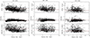 |
Fig. A.1. Radial variation of the dust attenuation in the Hα line derived using the Balmer decrement (upper panels), of the [N II] contamination (central panels), and their combined effect (lower panels; the Y-axis give the multiplicative factor which should be used to correct luminosities) for the three galaxies of the MUSE/PHANGS sample in common, NGC 4254, NGC 4321, and NGC 4535. The red dashed line shows the values derived using integrated quantities and used in this work, the black solid line the linear best fit to the data. |
Appendix B: Properties of the sample galaxies
The galaxies analysed in this work (unperturbed sample) are listed in Table B.1 along with their parameters. Table B.2 gives the parameters of the elliptical apertures used for the identification of the H II regions and for the extraction of the total Hα flux. Table B.3 lists the best-fit parameters for the luminosity function of individual objects.
Galaxies analysed in this work
Apertures used for the flux extraction and for the identification of the H II regions
Best-fit parameters of the fit of the luminosity function for individual galaxies
Appendix C: Scaling relations
C.1. Main scaling relations
In this Appendix we present all the scaling relations analysed in Sec. 4.2. These include the scaling relations between the total number of H II regions, the brightest H II region, their relative contribution to the total Hα luminosity of the target galaxies, as well as the best-fit parameters of the luminosity function of the H II regions and several physical parameters representing their hosting galaxies such as the star formation activity, the stellar mass, the mean star formation activity and stellar mass surface density, the metallicity, the molecular-to-atomic gas fraction, the gas-to-dust ratio, the specific star formation rate, and the morphological type. The parameters of the best fit are shown in the figures and given in Table 5 only whenever the probability P that the two variables are correlated with P ≥ 95% (p-value < 0.05).
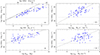 |
Fig. C.1. Relation between the Hα luminosity of the brightest H II region and the total star formation rate (upper left panel), total stellar mass (lower left), mean star formation rate surface density (upper right), and mean stellar mass surface density (lower right) of the host galaxies. The black dashed line shows the best fit to the data (bisector fit), the dotted line the limiting Hα luminosity of the selected sample (L(Hα) ≥ 1037 erg s−1), and the solid black line the L(Hα)1 ≤ L(Hα) physical limit in the relation. The dot in the lower right corner shows the typical error bar in the data. |
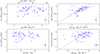 |
Fig. C.2. Relation between L(Hα)≥37/L(Hα), defined as the ratio between the sum of the Hα luminosity of all the H II regions with luminosity L(Hα) ≥ 1037 erg s−1 and the integrated Hα luminosity of the galaxy, and the total star formation rate (upper left panel), total stellar mass (lower left), mean star formation rate surface density (upper right), and mean stellar mass surface density (lower right) of the host galaxies. The dot in the lower right corner shows the typical error bar in the data. |
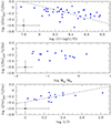 |
Fig. C.3. Relation between L(Hα)≥37/L(Hα), defined as the ratio between the sum of the Hα luminosity of all the H II regions with luminosity L(Hα) ≥ 1037 erg s−1 and the integrated Hα luminosity of the galaxy, and the metallicity (upper panel), the molecular-to-atomic gas ratio (central panel), and the total gas-to-dust ratio (lower panel) of the host galaxies. The black dashed line shows the best fit to the data (bisector fit). The dot in the lower left corner shows the typical error bar in the data. |
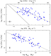 |
Fig. C.4. Relation between L(Hα)1/L(Hα) and the total star formation rate (upper panel) and total stellar mass (lower panel) of the host galaxies. The black dashed line shows the best fit to the data (bisector fit) and the solid black line the L(Hα)1 ≤ 1037 erg s−1 physical limit in the relation. The dot in the lower left corner shows the typical error bar in the data. |
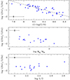 |
Fig. C.5. Relation between L(Hα)1/L(Hα) and and the metallicity (upper panel), the molecular-to-atomic gas ratio (central panel), and the total gas-to-dust ratio (lower panel) of the host galaxies. The black dashed line shows the best fit to the data (bisector fit). The dot in the lower left corner shows the typical error bar in the data. |
 |
Fig. C.6. Relation between the ratio of the total Hα luminosity of H II regions with L(Hα) ≥ 1037 erg s−1 (upper panel), of the brightest H II region (central panel), and of the sum of the Hα luminosity of the brightest three H II regions and the integrated Hα luminosity and the specific star formation rate of the parent galaxies. The black dashed line shows the best fit to the data (bisector fit). The dot in the lower right corner shows the typical error bar in the data. |
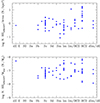 |
Fig. C.7. Relation between the number of H II regions of luminosity L(Hα) ≥ 1037 erg s−1 per unit disc size (upper panel) and stellar mass (lower panel) and the morphological type. |
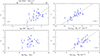 |
Fig. C.8. Relation between the faint end slope of the luminosity function α and the total star formation rate (upper left panel), total stellar mass (lower left), mean star formation rate surface density (upper right), and mean stellar mass surface density (lower right) of the host galaxies. The black dashed line shows the best fit to the data (bisector fit). The dots in the lower left and right corners show the typical error bar in the data. |
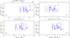 |
Fig. C.9. Relation between the characteristic luminosity of the luminosity function L* and the total star formation rate (upper left panel), total stellar mass (lower left), mean star formation rate surface density (upper right), and mean stellar mass surface density (lower right) of the host galaxies. The dots in the lower left and right corners show the typical error bar in the data. |
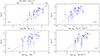 |
Fig. C.10. Relation between the characteristic number density of the luminosity ϕ* and the total star formation rate (upper left panel), total stellar mass (lower left), mean star formation rate surface density (upper right), and mean stellar mass surface density (lower right) of the host galaxies. The black dashed line shows the best fit to the data (bisector fit). The dots in the lower left and right corners show the typical error bar in the data. |
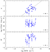 |
Fig. C.11. Relation between the faint end slope α (upper panel), the characteristic luminosity L* (central panel), and ϕ* (lower panel) of the luminosity function and the specific star formation rate of the parent galaxies. The black dashed line shows the best fit to the data (bisector fit). The dot in the lower right corner shows the typical error bar in the data. |
C.2. Scaling relations with the first three ranked H II regions
Often used in the literature are also the scaling relations with the mean (⟨L(Hα)3⟩) or the sum (L(Hα)3) of the first three ranked H II regions. These relations generally follow those found for the first ranked H II region presented in Sec. 4 and discussed in Sec. 5. For completeness, we include these relations in this Appendix. The best-fit parameters of these relations are given in Table 5.
Figure C.12 shows the relations between the mean Hα luminosity of the three brightest H II regions and the total star formation rate, stellar mass (and their surface densities) of the parent galaxies. The mean Hα luminosity of the three brightest H II region is tightly related to the star formation rate, stellar mass, mean star formation rate, and stellar mass surface density of their host.
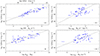 |
Fig. C.12. Relation between the mean Hα luminosity of the three brightest H II regions and the total star formation rate (upper left panel), total stellar mass (lower left), mean star formation rate surface density (upper right), and mean stellar mass surface density (lower right) of the host galaxies. The black dashed line shows the best fit to the data (bisector fit), the dotted line the limiting Hα luminosity of the selected sample (L(Hα) ≥ 1037 erg s−1). The dot in the lower right corner shows the typical error bar in the data. |
Figure C.13 shows the relation between L(Hα)3/L(Hα), the contribution of the three brightest H II region to the total Hα luminosity of the galaxy, and the integrated star formation rate and stellar mass of the host. Figure C.13 indicates that the contribution of the three brightest H II regions to the total Hα emission of galaxies strongly increases from ≃ 1-10% in star-forming (SFR ≃ 1 M⊙ yr−1) and massive (Mstar ≃ 1010 M⊙) objects to ≃ 50-100% in dwarf systems (SFR ≃ 10−3 M⊙ yr−1; Mstar ≃ 107 M⊙).
Figure C.14 shows the relation L(Hα)3/L(Hα) and the metallicity, the molecular-to-atomic gas ratio, and the total gas-to-dust ratio. The poor statistic (15 objects) prevents us to see whether the two variables are related to MH2/MHI and Mgas/Mdust, but clearly show an anti-correlation with the gas metallicity.
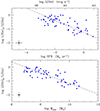 |
Fig. C.13. Relation between L(Hα)3/L(Hα) (contribution of the brightest three H II regions to the total Hα luminosity of the galaxy) and the total star formation rate (upper panel) and total stellar mass (lower panel) of the host galaxies. The black dashed line shows the best fit to the data (bisector fit). The dot in the lower left corner shows the typical error bar in the data. |
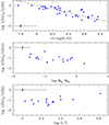 |
Fig. C.14. Relation between L(Hα)3/L(Hα) (contribution of the brightest three H II regions to the total Hα luminosity of the galaxy) and the total star formation rate (upper panel) and total stellar mass (lower panel) of the host galaxies. The black dashed line shows the best fit to the data (bisector fit), while the black dot the typical error in the data. |
Appendix D: Relation between the star formation rate and stellar mass surface densities
Two of the scaling parameters used in Sec. 4.2 to characterise the typical properties of the selected galaxies are the mean stellar mass and star formation rates surface densities as defined in eq. 6 and 5, respectively. These two quantities are tightly related, as shown in Fig. D.1. The bisector fit of the relation is: log μSFR [M⊙ yr−1 kpc−2] = 1.25±0.08 × log μstar [M⊙ kpc−2] -11.92±0.50 (ρ = 0.74, σ = 0.32). The strong relation between these two variables suggests that the star formation process is tightly connected to the stellar gravity of the disc (Shi et al. 2018). This relation is expected given that the two variables Mstar and L(Hα) are strongly correlated (main sequence relation, see Boselli et al. (2023a) for details on this relation in the VESTIGE sample). While the main sequence relation is an obvious scaling relation where "bigger galaxies have more of everything" (Kennicutt 1990), the one using normalised entities is more indicated to compare objects of different size and nature.
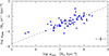 |
Fig. D.1. Relation between the mean star formation rate surface density and the mean stellar mass surface density. The black dashed line shows the best fit to the data (bisector fit). The dot in the lower right corner shows the typical error bar in the data. |
Appendix E: Luminosity function on individual objects
Figure E.1 shows the luminosity function of H II regions derived for the 27 galaxies of the sample with at least 20 H II regions detected by HIIPHOT above the completeness limit of the survey (L(Hα) ≥ 1037 erg s−1).
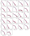 |
Fig. E.1. Luminosity function of the H II regions detected by HIIPHOT in individual galaxies. The Hα luminosity of individual H II regions is corrected for dust attenuation and [N II] contamination as described in Sec. 3.2. The solid blue and red lines indicate the best fit and 1σ confidence regions for the Schechter luminosity function parametrisation. Black solid dots indicate the number of H II regions in 0.25 dex bins of Hα luminosity above the adopted completeness of the survey (L(Hα) ≥ 1037 erg s−1). |
All Tables
Best-fit parameters for the luminosity-size relation (log L(Hα) = a × log Deq + b).
Apertures used for the flux extraction and for the identification of the H II regions
Best-fit parameters of the fit of the luminosity function for individual galaxies
All Figures
|
Fig. 1. Distribution of the H I-deficiency parameter for the parent sample galaxies. The blue histogram shows the distribution of the unperturbed systems with H I−def ≤ 0.4 and b/a ≥ 0.25 analysed in this work (64 objects, unperturbed sample), the red histogram the one of perturbed galaxies with H I−def > 0.4 and b/a ≥ 0.25 (258 objects, perturbed sample). The blue dotted vertical lines show the 1σ range distribution of the H I-deficiency parameter observed in isolated systems. |
| In the text | |
|
Fig. 2. Normalised seeing distribution in the HαNB (upper panel) and r-band (lower panel). At the distance of the Virgo cluster (16.5 Mpc), the mean values (indicated by a vertical arrow and given in parenthesis) correspond to 58 pc and 62 pc in the HαNB and r-band, respectively. |
| In the text | |
|
Fig. 3. Completeness function in luminosity of the H II regions detected by HIIPHOT for galaxies belonging to the different substructures of the cluster located at 15.8 (cluster B, C; magenta), 16.5 (cluster A, LVC; blue), 23 (W′ cloud; green), and 32 Mpc (W and M clouds; red), respectively. The vertical dashed line shows the limit in Hα luminosity adopted to define a complete sample where statistical properties are derived. The black arrows show how the position of a limiting Hα luminosity L(Hα) = 1037 erg s−1 should be shifted for a dust attenuation of A(Hα) = 1 mag or a [N II] contamination of [N II]/Hα = 0.5 (for reference, the measured values for NGC 4321 used for this test are A(Hα) = 0.85 mag and [N II]/Hα = 0.48). |
| In the text | |
|
Fig. 4. Relationship between the flux of individual H II regions of NGC 4254 extracted from the VESTIGE images and from the MUSE/PHANGS datacubes. For consistency with the MUSE data, the VESTIGE data are the output of HIIPHOT uncorrected for the diffuse emission. The lower panel shows how the ratio of the VESTIGE-to-PHANGS flux ratio changes as a function of the effective diameter corrected for seeing smearing. The vertical green dashed line corresponds to the seeing of the VESTIGE image, the vertical brown dashed line to the seeing of the MUSE/PHANGS dataset. Blue dots (orange circles) are for H II regions with more (less) than 50 pixels in the VESTIGE image (regions with a typical radius of ≃0.75″). The distributions of their ratio is given in the lower right panel. |
| In the text | |
|
Fig. 5. Relationship between the flux of individual H II regions of NGC 4321 extracted from the VESTIGE images and from the MUSE/PHANGS datacubes (see Fig. 4 for details). |
| In the text | |
|
Fig. 6. Relationship between the flux of individual H II regions of NGC 4535 extracted from the VESTIGE images and from the MUSE/PHANGS datacubes (see Fig. 4 for details). |
| In the text | |
|
Fig. 7. Composite luminosity function of the H II regions detected by HIIPHOT on the selected galaxies. The Hα luminosities of individual H II regions have been corrected for dust attenuation and [N II] contamination as described in Sect. 3.2. The solid and dotted lines indicate the best-fit and 1σ confidence regions for the Schechter luminosity function parametrisation. The vertical dashed line shows the completeness of the survey. The small panel in the top right corner indicates the 1σ probability distribution of the fitted Schechter function parameters. |
| In the text | |
|
Fig. 8. Composite luminosity function of the H II regions detected within (magenta) and outside (cyan) the i-band effective radius of the target galaxies normalised to the total number of H II regions with L(Hα)≥1037 erg s−1 within (Ntot = 4194) and outside (Ntot = 9084) the effective radius. The vertical dashed line shows the completeness of the survey. The small panel in the top right corner indicates the 1σ probability distribution of the fitted Schechter function parameters. |
| In the text | |
|
Fig. 9. Composite luminosity function of the H II regions detected by HIIPHOT on the selected galaxies. Different colours are used for galaxies belonging to different cluster substructures: cyan for cluster A and LVC, 16.5 Mpc; magenta for cluster B, 15.8 Mpc; green for W′ cloud, 23 Mpc; and red for W and M clouds, 32 Mpc. The Hα luminosities of individual H II regions are corrected for dust attenuation and [N II] contamination as described in Sect. 3.2. The solid and dotted lines indicate the best-fit and 1σ confidence regions for the Schechter luminosity function parametrisation. The vertical dashed line shows the completeness of the survey. The small panel in the top right corner indicates the 1σ probability distribution of the fitted Schechter function parameters. |
| In the text | |
|
Fig. 10. Relation between the faint end slope α of the luminosity function and the characteristic luminosity of individual galaxies with more than 20 H II regions brighter than L(Hα)≥1037 erg s−1. Different colours are used for galaxies belonging to different cluster substructures: cyan for cluster A and LVC, 16.5 Mpc; magenta for cluster B, 15.8 Mpc; green for W′ cloud, 23 Mpc; and red for W and M clouds, 32 Mpc. The Hα luminosities of individual H II regions are corrected for dust attenuation and [N II] contamination as described in Sect. 3.2. |
| In the text | |
|
Fig. 11. Distribution of the observed (black dots) and corrected for seeing effects (blue dots) equivalent diameters for H II regions with L(Hα)≥1037 erg s−1. The dashed vertical line shows the equivalent diameter corresponding to the mean seeing of the survey at the distance of the cluster (16.5 Mpc). |
| In the text | |
|
Fig. 12. Normalised distributions of the equivalent diameters corrected for seeing effects measured within (magenta) and outside (cyan) the i-band effective radius of the selected galaxies for H II regions with L(Hα)≥1037 erg s−1. The dashed vertical line shows the equivalent diameter corresponding to the mean seeing of the survey at the distance of the cluster (16.5 Mpc). |
| In the text | |
|
Fig. 13. Distribution of the equivalent diameters corrected for seeing effects equivalent diameters for H II regions with L(Hα)≥1037 erg s−1. The different colours are for galaxies belonging to different cluster substructures: cyan for cluster A and LVC, 16.5 Mpc; magenta for cluster B, 15.8 Mpc; green for W′ cloud, 23 Mpc; and red for W and M clouds, 32 Mpc. The dashed vertical lines show the equivalent diameter corresponding to the mean seeing of the survey at the distance of the different cluster substructures. |
| In the text | |
|
Fig. 14. Distribution of the electron density derived using equivalent diameters corrected for seeing effects for H II regions with L(Hα)≥1037 erg s−1 and a diameter correction factor ≤50%. |
| In the text | |
|
Fig. 15. Normalised distributions of the electron density derived using equivalent diameters corrected for seeing effects for H II regions with L(Hα)≥1037 erg s−1 for H II regions located inside (magenta) and outside (cyan) the i-band effective radius. The two distributions are normalised to the total number of regions located within and outside the effective radius. The number of H II regions with densities ne ≥ 7.5 cm−3 for the two samples are most one per bin but are plotted at different positions because of the different normalisation. |
| In the text | |
|
Fig. 16. Distribution of the electron density derived using equivalent diameters corrected for seeing effects for H II regions with L(Hα)≥1037 erg s−1 and a diameter correction factor ≤50%. Different colours are for galaxies belonging to the different Virgo cluster substructures (cyan for cluster A and LVC, 16.5 Mpc; magenta for cluster B, 15.8 Mpc; green for W′ cloud, 23 Mpc; red for W and M clouds, 32 Mpc). |
| In the text | |
|
Fig. 17. Relation between the Hα luminosity of individual H II regions corrected for [N II] contamination and dust attenuation and the equivalent diameter corrected for seeing effects. Blue filled dots are for H II regions with a diameter correction factor ≤50%, grey dots for all H II regions with no limits in diameter correction. The vertical dashed line shows the mean FWHM of the survey assuming galaxies at the distance of the main body of the cluster (16.5 Mpc). The blue solid line gives the bisector fit (Isobe et al. 1990) of the relation derived for H II regions with a diameter correction factor ≤50% (blue dots), the grey solid line for H II regions with no limits in the diameter correction. |
| In the text | |
|
Fig. 18. Relation between the Hα luminosity of individual H II regions corrected for [N II] contamination and dust attenuation and the equivalent diameter corrected for seeing effects for regions located within (right, filled magenta dots) and outside (left, filled cyan dots) the i-band effective radius of the parent galaxy, where the correction is less than 50%. Grey dots show all H II regions with no limits in luminosity and diameter correction. The vertical dashed line shows the mean FWHM of the survey assuming galaxies at the distance of the main body of the cluster (16.5 Mpc). The magenta and cyan solid lines give the bisector fit of the relations derived for galaxies with a diameter correction factor ≤50% (magenta and cyan filled dots). |
| In the text | |
|
Fig. 19. Relation between the Hα luminosity of individual H II regions corrected for [N II] contamination and dust attenuation and the equivalent diameter corrected for seeing effects. Coloured (cyan for cluster A and LVC, 16.5 Mpc; magenta for cluster B, 15.8 Mpc; green for W′ cloud, 23 Mpc; red for W and M clouds, 32 Mpc) dots are for H II regions with a diameter correction factor ≤50%, and the grey dots are for all H II regions with no limits in diameter correction. The vertical dashed lines show the mean FWHM of the survey assuming for the different substructures of the cluster. The coloured solid lines give the bisector fit of the relation derived for galaxies with a diameter correction factor ≤50%. |
| In the text | |
|
Fig. 20. Relation between the total number of H II regions detected by HIIPHOT with L(Hα)≥1037 erg s−1 and the total star formation rate (upper left panel), total stellar mass (lower left), mean star formation rate surface density (upper right), and mean stellar mass surface density (lower right) of the host galaxies. Star formation rates (lower axis) have been derived from Hα luminosities (upper axis) corrected for dust attenuation and [N II] contamination assuming a Chabrier IMF. The black dashed line shows the best fit to the data (bisector fit). The dot in the lower right corner shows the typical error bar in the data. |
| In the text | |
|
Fig. A.1. Radial variation of the dust attenuation in the Hα line derived using the Balmer decrement (upper panels), of the [N II] contamination (central panels), and their combined effect (lower panels; the Y-axis give the multiplicative factor which should be used to correct luminosities) for the three galaxies of the MUSE/PHANGS sample in common, NGC 4254, NGC 4321, and NGC 4535. The red dashed line shows the values derived using integrated quantities and used in this work, the black solid line the linear best fit to the data. |
| In the text | |
|
Fig. C.1. Relation between the Hα luminosity of the brightest H II region and the total star formation rate (upper left panel), total stellar mass (lower left), mean star formation rate surface density (upper right), and mean stellar mass surface density (lower right) of the host galaxies. The black dashed line shows the best fit to the data (bisector fit), the dotted line the limiting Hα luminosity of the selected sample (L(Hα) ≥ 1037 erg s−1), and the solid black line the L(Hα)1 ≤ L(Hα) physical limit in the relation. The dot in the lower right corner shows the typical error bar in the data. |
| In the text | |
|
Fig. C.2. Relation between L(Hα)≥37/L(Hα), defined as the ratio between the sum of the Hα luminosity of all the H II regions with luminosity L(Hα) ≥ 1037 erg s−1 and the integrated Hα luminosity of the galaxy, and the total star formation rate (upper left panel), total stellar mass (lower left), mean star formation rate surface density (upper right), and mean stellar mass surface density (lower right) of the host galaxies. The dot in the lower right corner shows the typical error bar in the data. |
| In the text | |
|
Fig. C.3. Relation between L(Hα)≥37/L(Hα), defined as the ratio between the sum of the Hα luminosity of all the H II regions with luminosity L(Hα) ≥ 1037 erg s−1 and the integrated Hα luminosity of the galaxy, and the metallicity (upper panel), the molecular-to-atomic gas ratio (central panel), and the total gas-to-dust ratio (lower panel) of the host galaxies. The black dashed line shows the best fit to the data (bisector fit). The dot in the lower left corner shows the typical error bar in the data. |
| In the text | |
|
Fig. C.4. Relation between L(Hα)1/L(Hα) and the total star formation rate (upper panel) and total stellar mass (lower panel) of the host galaxies. The black dashed line shows the best fit to the data (bisector fit) and the solid black line the L(Hα)1 ≤ 1037 erg s−1 physical limit in the relation. The dot in the lower left corner shows the typical error bar in the data. |
| In the text | |
|
Fig. C.5. Relation between L(Hα)1/L(Hα) and and the metallicity (upper panel), the molecular-to-atomic gas ratio (central panel), and the total gas-to-dust ratio (lower panel) of the host galaxies. The black dashed line shows the best fit to the data (bisector fit). The dot in the lower left corner shows the typical error bar in the data. |
| In the text | |
|
Fig. C.6. Relation between the ratio of the total Hα luminosity of H II regions with L(Hα) ≥ 1037 erg s−1 (upper panel), of the brightest H II region (central panel), and of the sum of the Hα luminosity of the brightest three H II regions and the integrated Hα luminosity and the specific star formation rate of the parent galaxies. The black dashed line shows the best fit to the data (bisector fit). The dot in the lower right corner shows the typical error bar in the data. |
| In the text | |
|
Fig. C.7. Relation between the number of H II regions of luminosity L(Hα) ≥ 1037 erg s−1 per unit disc size (upper panel) and stellar mass (lower panel) and the morphological type. |
| In the text | |
|
Fig. C.8. Relation between the faint end slope of the luminosity function α and the total star formation rate (upper left panel), total stellar mass (lower left), mean star formation rate surface density (upper right), and mean stellar mass surface density (lower right) of the host galaxies. The black dashed line shows the best fit to the data (bisector fit). The dots in the lower left and right corners show the typical error bar in the data. |
| In the text | |
|
Fig. C.9. Relation between the characteristic luminosity of the luminosity function L* and the total star formation rate (upper left panel), total stellar mass (lower left), mean star formation rate surface density (upper right), and mean stellar mass surface density (lower right) of the host galaxies. The dots in the lower left and right corners show the typical error bar in the data. |
| In the text | |
|
Fig. C.10. Relation between the characteristic number density of the luminosity ϕ* and the total star formation rate (upper left panel), total stellar mass (lower left), mean star formation rate surface density (upper right), and mean stellar mass surface density (lower right) of the host galaxies. The black dashed line shows the best fit to the data (bisector fit). The dots in the lower left and right corners show the typical error bar in the data. |
| In the text | |
|
Fig. C.11. Relation between the faint end slope α (upper panel), the characteristic luminosity L* (central panel), and ϕ* (lower panel) of the luminosity function and the specific star formation rate of the parent galaxies. The black dashed line shows the best fit to the data (bisector fit). The dot in the lower right corner shows the typical error bar in the data. |
| In the text | |
|
Fig. C.12. Relation between the mean Hα luminosity of the three brightest H II regions and the total star formation rate (upper left panel), total stellar mass (lower left), mean star formation rate surface density (upper right), and mean stellar mass surface density (lower right) of the host galaxies. The black dashed line shows the best fit to the data (bisector fit), the dotted line the limiting Hα luminosity of the selected sample (L(Hα) ≥ 1037 erg s−1). The dot in the lower right corner shows the typical error bar in the data. |
| In the text | |
|
Fig. C.13. Relation between L(Hα)3/L(Hα) (contribution of the brightest three H II regions to the total Hα luminosity of the galaxy) and the total star formation rate (upper panel) and total stellar mass (lower panel) of the host galaxies. The black dashed line shows the best fit to the data (bisector fit). The dot in the lower left corner shows the typical error bar in the data. |
| In the text | |
|
Fig. C.14. Relation between L(Hα)3/L(Hα) (contribution of the brightest three H II regions to the total Hα luminosity of the galaxy) and the total star formation rate (upper panel) and total stellar mass (lower panel) of the host galaxies. The black dashed line shows the best fit to the data (bisector fit), while the black dot the typical error in the data. |
| In the text | |
|
Fig. D.1. Relation between the mean star formation rate surface density and the mean stellar mass surface density. The black dashed line shows the best fit to the data (bisector fit). The dot in the lower right corner shows the typical error bar in the data. |
| In the text | |
|
Fig. E.1. Luminosity function of the H II regions detected by HIIPHOT in individual galaxies. The Hα luminosity of individual H II regions is corrected for dust attenuation and [N II] contamination as described in Sec. 3.2. The solid blue and red lines indicate the best fit and 1σ confidence regions for the Schechter luminosity function parametrisation. Black solid dots indicate the number of H II regions in 0.25 dex bins of Hα luminosity above the adopted completeness of the survey (L(Hα) ≥ 1037 erg s−1). |
| In the text | |
Current usage metrics show cumulative count of Article Views (full-text article views including HTML views, PDF and ePub downloads, according to the available data) and Abstracts Views on Vision4Press platform.
Data correspond to usage on the plateform after 2015. The current usage metrics is available 48-96 hours after online publication and is updated daily on week days.
Initial download of the metrics may take a while.