| Issue |
A&A
Volume 695, March 2025
|
|
|---|---|---|
| Article Number | A158 | |
| Number of page(s) | 16 | |
| Section | Planets, planetary systems, and small bodies | |
| DOI | https://doi.org/10.1051/0004-6361/202453072 | |
| Published online | 18 March 2025 | |
Polydisperse formation of planetesimals
The dust size distribution in clumps
Planetary Exploration, Technical University Delft,
Kluyverweg 1 2629 HS Delft,
The Netherlands
★ Corresponding author; This email address is being protected from spambots. You need JavaScript enabled to view it.
Received:
19
November
2024
Accepted:
31
January
2025
Abstract
Aims. To form kilometre-sized planetesimals, the streaming instability is an efficient method for overcoming the barriers to planet formation in protoplanetary discs. The streaming instability has been extensively modelled by hydrodynamic simulations of gas and a single dust size. However, recent studies considering a more realistic case of a particle size distribution have shown that this will significantly decrease the growth rate of the instability. We follow up on these studies by evaluating the polydisperse streaming instability in the non-linear regime to see if clumping can occur in the same manner as the monodisperse streaming instability and determine the size distribution in the densest dust structures.
Methods. We employ 2D hydrodynamic simulations in an unstratified shearing box with multiple dust species representing an underlying continuous dust size spectrum using FARGO3D. We use the Gauss-Legendre quadrature in dust size space to calculate the drag force on the gas due to a continuous dust size distribution. These simulations are compared to previous analytical results of the polydisperse streaming instability in the linear phase. We then look at the saturated non-linear phase of the instability at the highest density regions and investigate the dust size distribution in the densest dust structures.
Results. When sampling the size distribution, the error in the growth rate converges significantly faster with the number of dust sizes using the Gauss-Legendre quadrature method than the usual uniform sampling method. In the non-linear regime, the maximum dust density reached in the polydisperse case is reduced compared to the monodisperse case. Larger dust particles are most abundant in the densest dust structure because they are less coupled to the gas and can therefore clump together more than the smaller dust grains. Contrary to expectations based solely on dust-gas coupling, our results reveal a distinct peak in the size distribution that arises from the size-dependent spatial segregation of the highest-density regions, where particles with the largest Stokes numbers are located just outside the densest areas of the combined dust species.
Conclusions. The 2D unstratified polydisperse streaming instability is less efficient than its monodisperse counterpart at generating dense clumps that may collapse into planetesimals, and in the densest regions, the distinct dust size distribution could be related to the size distribution that ends up in the planetesimal and can mimic the size distribution of dust growth.
Key words: hydrodynamics / instabilities / methods: numerical / planets and satellites: formation / protoplanetary disks
© The Authors 2025
 Open Access article, published by EDP Sciences, under the terms of the Creative Commons Attribution License (https://creativecommons.org/licenses/by/4.0), which permits unrestricted use, distribution, and reproduction in any medium, provided the original work is properly cited.
This article is published in open access under the Subscribe to Open model. This email address is being protected from spambots. You need JavaScript enabled to view it. to support open access publication.
1 Introduction
Planets form in protoplanetary discs, where solid particles with sizes of around 0.1 μm need to clump together to form planetsized objects of around 10 000 km. However, this process is not trivial, and certain barriers impede the growth of the dust. At small sizes, the growth of the particles is dominated by collisional growth, which can lead to maximum dust sizes of approximately one centimetre, depending on local disc conditions (Birnstiel et al. 2011). The dust also feels a drag from the gas that orbits at sub-Keplerian velocities, which causes the dust to lose angular momentum and radially drift inwards towards the host star. The drift speed is dependent on the particle size such that for meter-sized objects, the drift timescale becomes shorter than the timescale of collisional growth, making it very difficult for particles to grow larger than one meter before they drift into the host star (Weidenschilling 1977; Nakagawa et al. 1986).
Radial drift can also trigger instabilities that can aid in dust growth. The relative velocities between the dust and gas can concentrate dust particles until densities exceed the threshold for gravitational collapse, leading directly to kilometre-sized bodies unaffected by fast radial drift. One of the most prominent drift-induced instabilities is the streaming instability (SI, e.g. Youdin & Goodman 2005; Youdin & Johansen 2007; Johansen et al. 2007; Nesvorný et al. 2019; Li & Youdin 2021). The SI has been extensively modelled using only a single dust size (monodisperse), either with a fluid-fluid or fluid-particle approach. More recent studies considering a more realistic case of a particle size distribution (first explored in Bai & Stone 2010) have also shown that this can dampen the instability in certain regimes (see Yang & Zhu 2021; Rucska & Wadsley 2023). Studies of the linear phase show that the polydisperse streaming instability (PSI) case will significantly decrease the growth rate of the monodisperse streaming instability (mSI) (Krapp et al. 2019; Paardekooper et al. 2020; Zhu & Yang 2021; McNally et al. 2021).
In this paper, we aim to build on the linear analysis of the PSI by investigating the non-linear regime and determining which dust sizes will end up in the overdensities formed by the instability during the saturated phase. This work is a continuation of three previous PSI papers (Paardekooper et al. 2020, 2021; McNally et al. 2021) focusing on the non-linear regime using hydrodynamical simulations.
Other studies of the PSI in the non-linear regime (Bai & Stone 2010; Yang & Zhu 2021; Schaffer et al. 2018, 2021; Rucska & Wadsley 2023) have covered a large part of the parameter space, evaluating PSI with a fluid-particle treatment, and have found dust clumps with densities exceeding the local Roche density, which may subsequently collapse into planetesimals. Yang & Zhu (2021) considered the non-linear evolution of the PSI using a discrete number of dust sizes. In this study, we take the dust size distribution to be a continuous limit using a fluidfluid treatment and only look at the high dust-to-gas ratio regime μ > 1 and smaller dust sizes that are well coupled to the gas. As in Yang & Zhu (2021), we ignore the vertical component of the stellar gravity and work in an unstratified local model of the disc. This simplified model allows us to make direct contact with linear theory (see Krapp et al. 2019; Paardekooper et al. 2020; Zhu & Yang 2021) and further our understanding of polydisperse drag instabilities. In this regime, we focus on the evolution of the dust size distribution to see if the PSI has a distinct size distribution at the highest density regions that could be related to the size distribution that ends up in planetesimals. This distribution could in turn be anchored to detailed observations of the Solar System (e.g. Mottola et al. 2015; Blum et al. 2017; Fulle & Blum 2017; Simon et al. 2018, 2022).
The heuristic model behind SI in the low dust-to-gas ratio regime μ < 1 is a resonant drag instability (RDI; Squire & Hopkins 2018b). The gas is supported by pressure. The forces and thus the acceleration of the gas are different from that of the dust. This leads to a drift velocity, δv, that causes an acceleration acting on the dust. In the Epstein regime (Epstein 1924), this acceleration, αdrag, d, is linearly dependent on the gas and dust velocity difference and the stopping time of the dust particles τs such that
 (1)
(1)
where a is the size of the particle, ρb is the bulk density of the dust particle, ρg is the gas density, and cs is the sound speed. This leads the terminal velocity of the dust to always be in the direction of the pressure maxima. This principle can be used to create overdensities that grow exponentially if there is a perturbation in the gas, and its wave velocity  matches the projected streaming velocity of the dust relative to the gas,
 (2)
(2)
with ws as the size-dependent velocity of dust relative to the gas and k as the wavenumber of the perturbation. The drag feedback on the gas increases the pressure maximum, leading to exponential growth if the projected wave velocity of the pressure perturbation is the same as the dust drift (Squire & Hopkins 2018a; Squire & Hopkins 2020; Magnan et al. 2024). From the definition of the RDI, it follows that the instability must be (1) unstable for all μ, (2) have growth rates maximised when the ‘resonant condition’ ws \cdot k=ω0 = Ω · k is satisfied, and (3) have a growth rate in the linear regime that scales as ℑ(ω) ∼ μ1/2 rather than μ. However, the drift velocity of the dust strongly depends on the dust size, making the RDI less effective for the distribution of dust sizes if there is no distinct resonant velocity (Krapp et al. 2019; Paardekooper et al. 2020, 2021; Zhu & Yang 2021; McNally et al. 2021)1.
There is a second regime at a high dust-to-gas ratio with higher growth rates where the PSI can grow. Importantly, the high-μ streaming instability is not an RDI and does not follow the RDI definitions from Squire & Hopkins (2018a). If the dust-togas ratio is higher than one (μ > 1), then there are fast-growing, high-k modes that are traditionally also called the ‘streaming instability’, but they are fundamentally different and share none of the RDI features and correlations that appear in low dust-togas ratio SI2. Instead, the high dust-to-gas ratio regime is more akin to a forced harmonic oscillator.
In this study, we aim to explore how different dust sizes clump together in the saturated regime of the instability and what the size distribution will be in the highest-density clumps. Section 2 discusses the governing equations in the local frame as well as the equilibrium state. In Section 3, we discuss the method of discretisation of size distribution and list the numerical setups of the simulations. In Section 4, we present the growth rates of different runs and compare their growth rates to analytical work. The non-linear regime and its properties are studied in Section 5 together with a convergence study. The simulations with different setups are used in a parameter study to investigate the effect of varying the diffusion coefficient, size distribution shapes, and dust-to-gas ratios in Section 6. In Section 7, we discuss how substructures arise within the densest clumps. In Section 8, we discuss the possible implication of the approximations we make, and we summarise our findings and the implication of the found substructures in the densest clumps on planet formation.
2 Polydisperse equations of motion
A numerical approach is necessary to study the PSI's nonlinear evolution. We can use the Euler equations that govern the evolution of the mixture and dynamics of the gas:
 (3)
(3)
 (4)
(4)
where p is the gas pressure, αg are the forces acting on the gas except the drag force of the dust denoted with αdrag, g.
We can take the velocity moments of the Boltzmann equation to derive the fluid equations that describe the evolution of the dust particles:
 (5)
(5)
 (6)
(6)
Here, u is defined as the size-dependent bulk velocity (u ≡ 〈vd〉v), σ the size density, and αd(u) the acceleration due to external forces and αdrag, d(u) from the drag between the dust and the gas (see, Paardekooper et al. 2021, for full derivation). In this derivation, we neglect the divergence of the stress tensor. This can only be done if we are in the regime of the fluid approximation. The fluid approximation is only valid for particles for which the coupling to the gas is strong enough, requiring Stokes number τs ≪ 1 (Garaud et al. 2004; Jacquet et al. 2011). Compared to the mSI, the backreaction on the gas is dependent on the size density σ, given by
 (7)
(7)
with V(a) the volume of the dust particle (V(a)=4 πa3/3 for spherical dust particles). The size density is the mass density between a and a + da, such that
 (8)
(8)
 (9)
(9)
with vd the bulk velocity of the dust. We can use these equations together with the definition of the acceleration of the dust αdrag, d to derive an expression for the total momentum transfer between the dust and gas:
 (10)
(10)
2.1 Local frame
We simulate the PSI within a shearing box (Goldreich & Lynden-Bell 1965), a co-rotating frame at an orbiting radius r0 with Cartesian coordinates
 . The transformation from the inertial frame will introduce inertial forces within the shearing box, the Coriolis and tidal forces. These forces are included through an effective potential Φ = −S Ω x2, with S the shearing rate, in a Keplerian disc
  with Ω the angular velocity. A global pressure gradient (∂P/∂r) exists throughout the disc in the local frame. This pressure gradient is described with the parameter3
 (11)
(11)
This means that the background acceleration on the gas, without the correction of the dust, can be given by
 (12)
(12)
Taking into account the equations from the frame transformation (12), momentum transfer (10) and the original equation governing the motions and mixture of gas and dust (3), (4), (5) and (6) will give the equations of motion within a shearing-box:
 (13)
(13)
 (14)
(14)
 (15)
(15)
 (16)
(16)
2.2 Equilibrium state
From the shearing box equations (13)–(16), we can find an equilibrium solution, this will indicate the radial drift and shear velocity of the gas and dust particles. We assume an isothermal equation of state, and all quantities are constant in space (apart from the shear) and have no vertical gravity (this is thought to represent the midplane of a protoplanetary disc). Then, the equilibrium solution is given by
 (17)
(17)
 (18)
(18)
 (19)
(19)
 (20)
(20)
 (21)
(21)
where κ is the epicyclic frequency and  is a series of integrals given by
 (22)
(22)
(from Paardekooper et al. (2020); first derived in Tanaka et al. 2005). These equations form the background solution in the shearing box.
2.3 Linear analysis
To evaluate the growth of the PSI, we need to have a perturbation on top of the equilibrium state that grows in the form of
 (23)
(23)
if we take the perturbation to be in the form of
 (24)
(24)
Here, k = (kx, ky, kz)T is the wavevector, and ω is the frequency. The growth rate of the perturbation is dependent on the imaginary part of the frequency, and the instability will grow if ℑ(ω) > 0. We can analytically determine the value of ω by solving the equations of motion (13)–(16) for (23). If we want to use these equations to solve for ω, this will constitute an integral eigenvalue problem for eigenvalue ω. This eigenvalue problem can be solved by either a discrete solver (Krapp et al. 2019) or by using a root finding method; both of these methods are described in Paardekooper et al. (2021) and an implementation in the publicly available Python package psitools4 (Paardekooper et al. 2020, 2021; McNally et al. 2021).
We want to further simplify the problem by only using dimensionless units by choosing a timescale Ω−1 and a length scale η/Ω2. When the timescale is Ω−1 the Stokes number is the non-dimensional stopping time St ≡ Ω τs, the parameters governing the system are now: the non-dimensional wave vector K = k η/Ω2, the non-dimensional sound speed cs/(Ω η), the shear parameter S/Ω, the dust-to-gas ratio μ = ρd0/ρg0 and the size density σ0 (a). We use the relation between Stokes number and dust size (1) to express the size density in the non-dimensional stopping time σ0(τs).
3 Numerical approach
We evaluate the non-linear regime with numerical simulation using the hydrodynamical code FARGO3D (Benítez-Llambay & Masset 2016; Benítez-Llambay et al. 2019) to evaluate the clumping of different dust sizes of the PSI.
3.1 Approximating the drag integral
FARGO3D allows for multiple dust fluids in a single simulation. In this multifluid picture, where a discrete number of dust sizes is considered, the backreaction on the gas is dictated by momentum conservation (Benítez-Llambay et al. 2019):
 (25)
(25)
where the sum is over all dust species, and subscripts j indicate quantities belonging to the jth dust species. In the polydisperse picture, where instead of a discrete number of sizes, we have a continuous size distribution, we can view the above equation as an approximation to the integral (10). This can be made explicit by defining ρd, j = σ (aj) Δ a, in the case of constant size bins of width Δa. The size distribution will usually span many orders of magnitude, in which case it is advantageous to choose size bins that have a constant size in log space, but the fundamental principle remains that the integral (10) is approximated by a (middle) Riemann sum or, in other words, the midpoint rule. This method is commonly used to approximate the drag integral (see e.g. Bai & Stone 2010; Krapp et al. 2019; Schaffer et al. 2018; Zhu & Yang 2021; Yang & Zhu 2021), and we henceforward refer to this method as the discrete method.
If we do not start with a multifluid approach, but assume from the start that we have a continuous size distribution, we need an accurate but robust way to calculate the drag integral (10). Without a priori knowledge about the integrand, GaussLegendre quadrature (GL) is a promising step forward from the midpoint rule. It is still convenient to work in log-size space, but rather than choosing bins of constant widths, the integration nodes are now given by the roots of the nth Legendre polynomial if we consider n integration nodes. If we, for simplicity, integrate over a rather than in log space, we have
 (26)
(26)
where wj are the GL weights and aj are the integration nodes, both appropriately adjusted for the integration range. If we compare (26) to (25), we see that if we define the dust densities as the product of the size density at the integration node and the corresponding weight, the equations are identical. This means that the GL integration method can be implemented in all hydrodynamics codes using pressureless fluids by choosing the appropriate sizes and redefining dust densities. Importantly, no changes in the internal workings of the code are necessary.
We can define the appropriate size and redefined dust densities with scipy.special.roots_legendre (Virtanen et al. 2020). This function gives the roots of the Legendre polynomial xj and weights wj between [−1; 1]. If we want to work in logsize space, we can map these notes to the correct Stokes number using
 (27)
(27)
and the redefined dust density by
 (28)
(28)
We give an example of the differences between the integration methods in Figure 1 by integrating a log-normal distribution using five points with the discrete and the GL method. The integration error using the discrete method is 8.292% and 0.018% using the GL method. This error will be smaller when using more integration points, but GL is more accurate using fewer integration points, which is less computationally expensive.
It is worth noting that, while GL and the discrete method have the same form, they differ fundamentally. When using GL, we let go of the concept of size bins: all we have is integration nodes. While the sum over all dust ‘densities’ ρd, j = wj σ(aj) gives the total dust density, as in the discrete case, this does not hold for partial sums. In other words, the GL method is optimised for integrating over the full-size distribution.
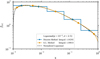 |
Fig. 1 Integration of a normalised log-normal distribution (dashed line) using a discrete method (blue line) and a Gauss-Legendre quadrature (orange line). |
3.2 The initial size distribution
The size distribution σ(a) in a protoplanetary disc can be expected to be inherited from the interstellar medium. The particle size distribution of the interstellar medium follows a power law given by MRN distribution (Mathis et al. 1977; Draine & Lee 1984):
 (29)
(29)
A power law will also follow from collisional evolution if we expect pure fragmentation or pure coagulation, making it a reasonable approximation for the size distribution when studying the PSI (e.g. used in Krapp et al. 2019; Paardekooper et al. 2020; McNally et al. 2021; Yang & Zhu 2021). When using dimensionless units to set up the simulations, the size distribution will be expressed in non-dimensional stopping time (Stokes number) τs, the stopping times can be converted back to dust sizes using (1) and a disc model, e.g. as a rough guide, a meter-sized boulder orbiting in the Minimum Mass Solar Nebula (MMSN) at one Astronomical Unit (AU) has a Stokes number of order unity (Weidenschilling 1977).
In our numerical study of the PSI, we want to explore a similar parameter space as was covered in the analytical analysis of the PSI in the linear regime by McNally et al. (2021).
For our standard case, we stay in the high-μ regime and take the dust-to-gas ratio μ = 3, although we vary this later (see Section 6.4).
The largest Stokes number τs, max in the distribution needs to be small enough that the fluid approximation holds. This approximation breaks down for τs ≳ 1 Ω−1; therefore, we take τs, max = 10−1 Ω−1. Although the dust size distribution in a protoplanetary disc can cover orders of magnitude, the error in the back-reaction of the dust is dependent on the sample rate of the distribution and is dominated by the larger dust sizes. Therefore, we sampled O(2) with τs ∈ [10−3; 10−1] Ω−1 (similar to the Stokes range in run Af and As in Yang & Zhu 2021).
3.3 Setup
We simulated the PSI with a shearing box in two spatial dimensions  , where the vertical stellar gravity is neglected (unstratified and isothermal). This means that the boundaries of the shearing box can be periodic. The background velocities of the gas and dust are given by the equilibrium solution (17)–(22). The gas and dust densities and velocities are perturbed by a small wave given by
 (30)
(30)
The amplitude  for all simulations5, the nondimensional wavenumber K = (30, 0, 30)T (from Figure 9 in McNally et al. 2021 we know that at this wavenumber the instability grows ℑ(ω) > 0, even if there is viscosity α) and
  are the 4(N + 1)-dimensional (complex) eigenvectors. These eigenvectors are associated with the (complex) eigenvalue ω(K, α, σ) and the (complex) mode frequency ω is calculated for a specific wave number K and viscosity parameter α with psitools.psimode. This setup is the same as the test problem LinA from Youdin & Johansen (2007).
The size of the shearing box is given in terms of the non-dimensional wavenumber Lx, z = 2 π/Kx, z. In this study, we perturb the system with one wavenumber and take the size of the box to be the length of the wave (Lx, z = 2 π/30 η/Ω2). The spatial resolution of the hydro-code is an important parameter of convergence; the linear regime of the instability only needs modest spatial resolution, e.g. only needing 4 × 4 for mSI. However, in a non-linear regime, the spatial resolution governs the limit of the smallest resolved clumping and maximum density. The spatial resolution is therefore always a compromise between accuracy and computation time. In this study, we do a larger parameter sweep at a resolution of 256 × 256 and a convergence study up to a resolution of 1024 × 1024. The specific combination of spatial resolution Ngrid, number of dust species nd and other parameters for different simulations are defined in Table 1.
List of simulation runs.
4 Linear regime
The perturbation will first grow exponentially (24), where the growth rates of the SI are dependent on the wavenumber, diffusion and size distribution ℑ(ω(K, α, σ)). This growth has an analytical solution that can be calculated with software package psitools (Paardekooper et al. 2020, 2021; McNally et al. 2021). We compare the analytical growth rates with those from the numerical simulations. The analytical growth rate can be determined from the frequency ω (24); for the polydisperse case ωPSI = 0.42030787 + i 0.04858883 and for the monodisperse case ωmSI = 0.34801869 + i 0.4190302. The time evolution of perturbations amplitude for a wave is shown in Figure 2A. The amplitude is calculated with a Fast Fourier Transform (with the software package SciPy; Virtanen et al. 2020). This amplitude can determine a growth rate corresponding to the numerical approach before it transitions into the non-linear regime for our runs. This happens at Ωt ∼ 125 for PSI runs and Ωt ∼ 30 for the mSI runs. In Figure 2, the coloured solid lines correspond to individual dust species at different Stokes numbers for the polydisperse case PSI 101024, and the dotted line is the amplitude of the sum of the dust species. The monodisperse dust species at τs = 0.1 Ω−1 is shown as a dot-dashed line. The growth rates and error between the analytical and numerical growth rates are given in Table 2.
In the linear regime, it is a lot easier to converge with spatial resolution than with the number of dust species (see Krapp et al. 2019; Zhu & Yang 2021). The error in the growth rate is an indication of how good the sampling method approximates the continuum limit of the integrated momentum transfer between the gas and dust (10). The error in the momentum transfer in the linear regime depends mainly on three parameters, the number of dust species used to sample the size distribution, the sampling method, and the spatial resolution. When we use the GL method, the error in the growth rate compared to the analytical value already converges between nd = 5 and 10, see Table 2. This is also visible if we show the amplitude growth of the largest wavevector K=(30, 0, 30) between the GL method and the discrete method, see Figure 3. In this Figure, the GL method (solid line) agrees with analytical results from psitools for both nd = 10 and 20. While the amplitude of the discrete method (dotted line) also converges with the analytical results, they are significantly less accurate than the GL method at the same number of dust species. Using the discrete sampling method, the error in the growth rate at nd = 40 is similar to the error using the GL method when using only nd = 5 (Table 2), which is a lot less computationally expensive to run.
The growth rate is also dependent on the maximum Stokes number, this is visualised in the top plot in Figure 4. The analytical growth rates calculated with psitools are visualised with the solid lines. We see that the growth rates decrease for lower Stokes numbers and are always lower for PSI than mSI. Even if we compare the growth rate of the mSI at the average Stokes number of a PSI size distribution, the growth rate of PSI is still smaller. For the specific example of the PSI with τs, max = 0.1 Ω−1, which has an average Stokes number  , the mSI growth rate is still 2.803 times higher than the growth rate of the PSI. The Stokes number of the mSI would have to be τs = 0.0321 Ω−1 to have a similar growth rate as the PSI.
The fitted values of the growth rates of the numerical runs agree well with the analytical growth rates in the top plot of Figure 4 for τs, max ≳ 0.035 Ω−1. For lower τs, however, we see the fitted mSI growth rates (red diamonds), start to deviate from the analytical growth rates (orange line). This can be explained by faster growing high-K modes; these get excited by small numerical errors and can boost the power P(K) at wavenumber K = (30, 0, 30)T and can even become the largest perturbed mode before the instability reaches the non-linear regime. This happens for runs mSIτs ≤ 0.035, run PSIτs, 5e−2, and run PSIβ,−3.8. This is also visible in the time evolution of the amplitude, where the amplitude suddenly increases a lot faster, such as the blue line in the top plot of Figure 14.
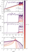 |
Fig. 2 Time evolution of the mSI (run: mSI1024) and PSI (run: PSI101024). The dot-dashed line shows the mSI run, the solid lines show the ten individual dust species of the PSI run, and the dotted line is the sum over all the dust species. Plot A shows the amplitude of the largest mode in the shearing box (A sinusoid with wavenumber K = (30, 0, 30)T), plot B shows the maximum density in the shearing box, plot C shows the mean density at every snapshot's 99th percentile and plot D shows the average probability density function of the normalised density distribution in the non-linear regime between (140 ≤ Ωt ≤ 160). |
Growth rates.
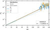 |
Fig. 3 Normalised amplitude of the largest mode of the shearing box (a sinusoid with a wavenumber K=(30, 0, 30)T) for different numbers of dust species and sampling methods. The runs with ten dust species are shown in blue, 20 dust species are shown in orange, and 40 dust species are shown in green. The solid line indicates the GL method (27), and the dotted line indicates a log-linear sampling method (runs: PSI20, PSI10, PSI40disc., PSI20disc., and PSI10disc..). The dot-dashed line is an analytical solution of the growth rate calculated with psitools. |
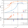 |
Fig. 4 Efficientcy of dust compression as a function of Stokes number. The top plot shows the growth rate in the linear regime at wavevector K = (30, 0, 30)T for setups with different maximum Stokes numbers τs, max. The solid orange and blue lines are the analytical growth rates (for mSI and PSI, respectfully) calculated with psitools (McNally et al. 2021). The diamonds indicate the fitted values of the growth rate in the linear regime of the numerical simulations. In the bottom plot, the diamonds correspond to the fitted values of the saturated amplification factor of the maximum density in the non-linear regime. The solid grey lines indicate the values for run PSI10, and the dotted grey line indicates the average Stokes number of the size distribution of run PSI10. |
5 Non-linear regime
When the amplitude of the perturbation gets high enough, the wave will break and transition to a turbulent non-linear state, showing vortices-like motion in the x,z-plane. Even though the non-linear regime is not analytically tractable, the fact that it saturates allows us to quantify it statistically; therefore, we can extract trends from this regime. The important feature is that the non-linear regime will produce high-density structures. This is also important for planet formation because the high-density structure can lead to clumping when we include self-gravity, and then the dust clumps can collapse into planetesimals when the Roche density is exceeded (see, e.g. the strong clumping criteria of Li & Youdin 2021). The extent of the trapping in the monodisperse case depends on the spatial resolution and Stokes number because we consider the dust to be a pressureless fluid with no diffusion. The spatial resolution in a grid-based hydrodynamical code determines the minimum size of structures that can be resolved. This also puts a constraint on the size of the clump, and larger clumps will have smaller maximum densities; the convergence of spatial resolution is further discussed in Section 5.2.1.
We expect higher dust densities for species with higher Stokes numbers since smaller dust is strongly coupled to the gas, which in turn is (nearly) incompressible. This means that the density distribution for smaller dust sizes will be more homogeneous, affecting the amplification factor for monodisperse distributions, see the bottom plot in Figure 4. In this plot, we can see that the amplification factor of the maximum density becomes lower for lower Stokes numbers. This is also the case for the individual dust species in PSI runs, where the smaller dust sizes are distributed more homogeneously. In Figure 5, we look at a snapshot of the normalised density for all the combined dust and the different dust sizes of run PSI101024, where we can see that the dust sizes are correlated; low-density and high-density regions occur in the same place for different dust species. The figure also shows that the amplification factor is lower for the smaller dust species. The normalised density for the largest dust bins shows more structure than the smallest species and is also visible if we plot the time evolution of the maximum density and the time-averaged density distributions, see Figure 2B and D, respectively. In Figure 2B, the dot-dashed line shows the monodisperse case from run mSI1024 and the solid line the individual dust species, where the colour indicates the Stokes number and the average Stokes number of the sum of the size distribution. In this figure, we can see that the amplification factor for mSI is largest at 484 ± 324. The amplification factor of the PSI is significantly lower at 27.3 ± 4.6.
Considering the strong τs dependence of the SI, comparing monodisperse and polydisperse simulations with a monodisperse τs equal to the maximum of the dust distribution of the corresponding polydisperse distribution is expected to yield higher dust densities in the monodisperse case, see bottom panel of Figure 4. Correcting for this bias, comparing polydisperse simulations to monodisperse ones with a τs equal to that of the average of the size distribution still shows higher dust densities in the monodisperse case. For the specific example with run PSI10, the average Stokes number is  . At this Stokes number, the mSI amplification factor of the maximum density is still 3.5 times higher than the amplification factor of run PSI10. The Stokes number of the mSI would have to be τs = 0.02 Ω−1 to have a similar amplification factor. This means that a PSI can not be represented by an mSI run with properties that are derived from the averaged properties of the PSI setup, such as the average Stokes number and total dust density of the size distribution.
The PSI is not a simple summation of individual discrete mSI cases at different Stokes numbers. One way the PSI differs from mSI is in terms of growth rates. The growth rates of all the individual dust species are identical for the PSI case, but this depends on the Stokes numbers in the mSI case, see Section 6.2. This also translates into the transition time of the individual dust species of the PSI. They all transition simultaneously (see Figures 2A–C), whilst the transition time mSI changes with Stokes numbers (however, the shared point of transition for PSI is also different for different Stokes ranges, see Section 6.2). There are also differences between discrete mSI cases and individual dust species of the PSI. The amplification factor is lower than the mSI case, and if (see Figure 5). The dust sizes are correlated; low-density and high-density regions occur in the same place for different dust species.
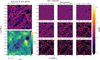 |
Fig. 5 Snapshot of the normalised density in the non-linear regime (Ωt = 166) for the PSI run PSI101024. The figure shows the density of the sum of the dust species (upper left), gas (lower left), and nine of the ten individual dust species with an increasing Stokes number.) |
5.1 The size distribution in the clumps
In Figure 2B, we can see that when considering the maximum dust density, the amplification factor increases monotonically with τs, as expected from linear theory and non-linear monodisperse simulations. However, in Figure 2C, we plot the mean of the top 1% of the dust density. We see that the trend is subtly different: the dust density increases with τs for most of the Stokes number range, but the maximum density occurs at τs, slightly smaller than the maximum. Since the top 1% of the dust density probes more extended structures than the absolute maximum dust density, this indicates that there is a peak in the size distribution in the clumps.
We can better visualize this peak in the size distribution by plotting the size distribution σ(τs). In Figure 6, we show the time evolution of a polynomial that passes through the GL points of PSI simulation (from run PSI101024) throughout the simulation. The top panel of Figure 6 shows size distribution at the 99th percentile, with the dotted line indicating the MRN size distribution at the start of the simulation. The bottom panel shows the same size distribution normalised by the background distribution and has a subplot zoomed at smaller densities.
The size distribution in the non-linear regime (Ωt > 125) settles into a trend with increasing densities at higher τs, but shows a clear peak. The peak in the size distribution could indicate either a resonance corresponding to the drift velocity or an inherent dependence on the Stokes range. From the mSI theory of the RDI, we can expect a strong response at size densities where the radial phase velocity of the perturbation matches the background radial drift velocity at a certain Stokes number:
 (31)
(31)
The PSI does not have this simple response with size distribution because of the distribution of dust sizes. There is a range of radial drift speeds ux (see Eq. (19)) dependent on the dust size, whilst the resonance can only be satisfied by a single velocity. However, we can use equation (9) and (19) to find the mean radial drift speed  of the size distribution. The mean drift velocity can be compared to the mSI drift speed vdx0(τs) where we define a resonance size τs where
  holds (from Paardekooper et al. 2021). In Figure 6, the Stokes number corresponding to this response is indicated with a vertical dashed line, and the average Stokes number
  is indicated with the dot-dashed line. The peak of the size distribution visually overlaps with the resonance size but does not convincingly correspond to it. On the other hand, the peak in the size distribution can be an inherent feature of the Stokes number range and is affected by the maximum Stokes number τs, max.
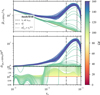 |
Fig. 6 Top: mean size distribution in the 99th percentile at different times. The dotted line indicates the size distribution at Ωt = 0. Bottom: same size distribution normalised by the background-size distribution σ0(τs). The dashed line indicates the Stokes number corresponding to the resonant velocity, and the dot-dashed line is the average Stokes number of the size distribution at Ωt = 0. |
5.2 Convergence
It is also possible that the peak in the size distribution corresponds to a numerical error. If this is the case, the peak should depend on the spatial resolution or the number of dust species used to sample the continuum size distribution. Another possibility is that the polynomial interpolation through the density of the individual dust species at the Stokes numbers that are sampled through the GL points will appear to indicate a peak, whilst the densities of the discrete dust species do not indicate this. We can validate this by using a larger number of dust species as well as comparing the GL method to the discrete method.
5.2.1 Spatial resolution
The spatial resolution directly limits the smallest structures that can be resolved within the simulation and the maximum density that is possible to create through clumping. Together with the fact that the dust fluid is fully compressible (unlike the gas), the simulations will never converge with spatial resolution unless dust diffusion is implemented, see Section 6.1. The dust without diffusion can be compressed into arbitrarily small volumes, and the maximum density in the non-linear regime will increase with increasing spatial resolution. This increase in density is not as strong if we look at the mean of larger percentiles. This is visible in Figure 7, showing the amplification factor for the mSI and PSI simulations at a spatial resolution of 256, 512 and 1024. For the PSI runs, the saturated mean density at the 99th percentile and maximum density increases with resolution, although the difference between resolutions is less at the 99th because we are analyzing larger structures. The linear regime of the PSI and mSI is not affected by the resolution, and the transition from the linear regime to the non-linear regime happens at the same time for different spatial resolutions, indicating that the linear regime already fully converged before a spatial resolution of 256 × 256 (Table 2). The amplification factor of the 99th percentile in the saturated regime for a resolution of mSI512 is lower than at a resolution of mSI256, this is counter-intuitive but not significant. The error is smaller than the 1 − σ variation of density, and the maximum density of mSI512 is higher than mSI at a Ngrid = 2566.
The overall shape of the peak in the size distribution in the highest density regions is consistent between resolutions, shown in Figure 8. The height of the size distribution increases slightly at higher Stokes numbers. At higher resolutions, the maximum amplification factor increases; therefore, 99th percentile covers less area, decreasing the relative presence of smaller Stokes numbers that are more homogeneously distributed around the shearing box. This is also why the size distribution is flatter when we average over the 90th percentile (also shown in Figure 8). We average over a larger area, where the smaller, more homogeneous dust species are relatively more abundant compared to the higher Stokes numbers that are more clumped. The simulations follow the relation between the overabundance of larger Stokes numbers in the highest-density regions and spatial resolution, but the peak (underrepresentation of the largest Stokes numbers) also stays consistent with different resolutions. There is a weak trend in the position of the peak to drift to smaller stroke numbers with higher resolution, although the change in Stokes number is a lot smaller than the difference between different-sized dust species.
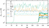 |
Fig. 7 Normalised (mean) density at the densest pixel and at the 99th percentile (indicated by darker and lighter colours; respectively) for different spatial resolutions. The mSI runs at different resolutions are indicated with the dotted line for run mSI1024, mSI512, and mSI using green, orange, and blue, respectively. The PSI runs PSI101024, PSI10512, and PSI10 have the same colour coding as the mSI runs. |
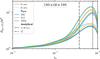 |
Fig. 8 Normalised mean size distribution at the 99th and 90th percentiles and between 140 ≤ Ωt ≤ 160 using the same PSI runs and colour scheme as Figure 7. |
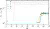 |
Fig. 9 Normalised mean density at the 99th percentile for different numbers of dust species from run mSI1024 (indicated with a dotted pink line), run PSI511024 (in blue), run PSI101024 (in orange), and run PSI201024 (in green). |
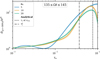 |
Fig. 10 Normalised mean size distribution at the 99th percentile and between 135 ≤ Ωt ≤ 145 using the same PSI runs and colour scheme as Figure 9. The dashed line indicates the Stokes number at resonance velocity |

5.2.2 Number of dust species
There are no big differences between simulations at different numbers of dust species in the linear regime (Section 4), but Figure 9 does show that the transition point from the linear regime to the non-linear regime shifts slightly with nd = 10 being slightly earlier and nd = 20 slightly later. The fact that the smallest sample rate is in the middle does not indicate any clear trend, but this can also be that nd = 5 is still far from converging. Because the saturation level between nd = 10 and nd = 20 is similar, whilst the saturated amplification factor of nd = 5 is significantly higher.
Figure 10 shows that mean size distribution in the 99th percentile does not show any clear correlation between dust sizes for nd = 5 except an increased abundance of larger Stokes numbers. There is a clear peak in the size distribution at nd = 10 and nd = 20, where the peaks appear to be more skewed at a higher sampling rate of nd = 20 compared to nd = 10. Although this sharper drop at the largest Stokes numbers does not appear for nd = 20 at a lower spatial resolution of 256 × 256, see Figure 11.
The size distribution remains smooth in size space for an increasing number of dust species, indicating that the GL method is also a good approximation for the continuum in the non-linear regime.
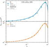 |
Fig. 11 Normalised mean size distribution at the 99th percentile and between 150 ≤ Ωt ≤ 200. The top plot shows the PSI run with ten dust species sampled from the GL in blue (run PSI10) and the PSI run with ten dust species uniformly sampled from a logarithmic scale in green (run PSI10disc.), and the bottom plot shows the PSI run using 20 dust species sampled from the GL in orange (run PSI20) and the PSI run with 20 dust species uniformly sampled from a logarithmic scale in pink (run PSI2 θdisc.). |
5.2.3 Sampling method
As discussed in Section 3.1, the GL approximates the integral for the impulse transfer between the dust species and the gas (10) is different from the uniform sampling method in logspace, that we defined as the discrete method. The error between the continuous limit and discrete integral decreases faster with the number of dust species using the GL method than using the discrete method, see Section 4.
The effect of the GL sampling method in the non-linear regime is less straightforward because the local size distribution can change significantly. It is possible that the size distribution can become more monodisperse locally and that the back reaction on the gas will be dominated by only part of the size distribution. This could affect the integration error. It is also possible that the peak in the size distribution in the densest regions could be an artefact of the weights or location of the roots of the polynomial or the projection of roots xi between [−1; 1] to the Stokes numbers τs, i within the Stokes range [τs, min; τs, max.], given by (27) and (28). Therefore, we reconstructed the size distribution of the simulation from the discrete method (run PSI10disc. and PSI20disc..) and compare it to the GL method, shown in Figure 11.
In the case of 10 dust species (Figure 11 top panel), the slight offset between the values of Stokes numbers of the two sampling methods means that the discrete sampling (shown in green) of the individual dust bins does not sample the size distribution at Stokes numbers larger than the peak. Therefore, we cannot conclude if there is a peak in the size distribution by looking at nd = 10, but the discrete method does follow the same general trend of the GL sampling method and are not in disagreement.
At a higher dust sampling rate of nd = 20 (Figure 11 bottom panel), where the discrete distribution does sample Stokes numbers larger than the peak, we see at least a reduced presence of the largest Stokes number that is consistent with the peak in the size distribution seen in all the simulation runs using the GL sampling method. This shows that the peak in the size distribution in the densest regions is physical rather than a numerical artefact.
6 Parameter study
To get a better indication of where the peak of the size distribution comes from and what can influence its location, we did a parameter study where we covered different values for the dust diffusion coefficient α, maximum Stokes number τs, max, the slope of the size distribution β and the dust-to-gas ratio μ, see Table 1. This parameter study is done at a fixed spatial resolution of Ngrid = 256 and using 10 dust species for the polydisperse simulations.
6.1 Diffusion
The diffusion coefficient α is a dimensionless parameter that quantifies the strength of the turbulence in protoplanetary discs and the viscosity v = αcsH. (Shakura & Sunyaev 1973). We used the α coefficient for the gas and dust diffusion in FARGO3D. The dust diffusion is modelled with a continuity equation for (pressureless) dust fluids, spreading mass depending on the gradient of the concentration (see appendix of Weber et al. (2019) for the implementation in FARGO3D).
Turbulence in a protoplanetary disc stirs the dust and can work to concentrate or disperse it, making it possible to form local regions of higher dust densities but also to destroy the formed substructure and clumps (Johansen et al. 2007; Yang et al. 2018; Schäfer et al. 2020; Lim et al. 2024a). The diffusion coefficient is important for addressing the finite resolution of hydrodynamical grid codes, where implementing a dust diffusion model can be a solution to the infinite compressibility of dust in the simulations and the unresolved turbulence. An important caveat is that the alpha model is limited on the small scales and can not capture the turbulence concentrating effect.
In the linear regime, the growth rates get smaller when the diffusion coefficient increases for the mSI (see analytical work of Youdin & Goodman 2005; Umurhan et al. 2020; Chen & Lin 2020) and for PSI (see McNally et al. 2021). The growth rates are shown in the top plot of Figure 12, for runs [mSIα, 1e−8, mSIα, 1e−7, mSIα, 1e−6, PSIα, 1e−8, PSIα, 1e−7, PSIα, 1e−6] where for the last polydisperse run with α = 10−6 there is no exponential growth and PSI does not develop. The lower plot shows that diffusion also affects the amplification factor of the SI, lowering the amplification factor for higher values of diffusion coefficients. The densities corresponding to the 99th percentile are also more variable in time at higher diffusion coefficients.
The peak in the size distribution exists for all diffusion coefficients where the PSI was able to form clumps (Figure 13). This means that the peak is independent of numerical or physical effects at the smallest scales, which are strongly damped by diffusion.
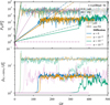 |
Fig. 12 Time evolution of the mSI (runs: [mSI*, mSIα,1e−8, mSIα,1e−7, mSIα,1e−6]) are shown with dotted lines and PSI (runs: [PSI*, PSIα, 1e−8, PSIα,1e−7, PSIα, 1e−6]) are shown with solid lines for different dust diffusion coefficients α. The colour indicates the diffusion coefficient, where no diffusion is shown in blue, α = 10−8 in orange, α = 10−7 in green, and α = 10−8 in pink. The top plot shows the amplitude of the largest mode in the shearing box (A sinusoid with wavenumber Kx,z = 30), and the dashed lines and dash-dotted lines show the analytical results calculated with psitools for the corresponding α. The bottom plot shows the normalised mean density at the 99th percentile for every snapshot. |
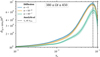 |
Fig. 13 Normalised mean size distribution at the 99th percentile and between 380 ≤ Ωt ≤ 450 for a dust diffusion coefficient of α = 0 (run PSI1Q) in blue, α = 10−8 (run PSIα,1e−8) in orange, and α = 10−7 (run PSIα,1e−7) in green. |
6.2 Stokes range
The larger dust species have a bigger impact on the momentum transfer of the PSI. This means that the location of the discontinuous upper boundary of the size distribution will impact the PSI. For the mSI, the Stokes number influences the growth rate, lower Stokes numbers have lower growth rates, see top plot of Figure 14. This trend is also visible for the PSI, but the run PSIτs, 5e−2 did not grow at the perturbed wave of Kx,z = 30, although around a time of 90 Ωt there is growth. This could be explained by small numerical errors that excite a different wavenumber K than the initial perturbation that does have a higher growth rate. The saturated amplification factor is not strongly affected by the upper boundary of the size distribution (bottom plot Figure 14).
Changing the maximum Stokes number τs,max will affect the size distribution in the upper 99th percentile. The peak of the size resolution in standard run PSI10 lies outside of the Stokes range of run PSIτs, 5e−2, but in this run, we still observe a peak in the distribution now at a different location. This means that the peak location is dependent on the initial size distribution and is always slightly smaller than the maximum Stokes number and thus dependent on τs,max. Changing the Stokes range also changes the bulk properties of the distribution, such as the average Stokes number  and the average drift velocity
  . The bulk drift velocity corresponds to a resonance size τs where
  , see Section 5.1. This resonance size changes for the different Stokes ranges and is indicated with a vertical dashed line in Figure 15. The location of the peak could also depend on the resonant size. Distinguishing between the resonant size and maximum Stokes number cannot be done by only changing the range of Size distribution, but we change the resonant size without changing the maximum Stokes number by changing the slope of the size distribution (Section 6.3). Another thing to take into account is that if the maximum Stokes number of the size distribution gets close to unity or even higher, the fluid approximation of the dust particles may not hold anymore.
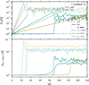 |
Fig. 14 Time evolution of the mSI (runs: [mSI*, mSIτs,5e−2, mSIτs,2e−1]) are shown with a dotted lines and PSI (runs: [PSI*, PSIτs,5e−2, PSIτs,2e−1]) are shown with solid lines for different peak Stokes numbers τs,max. The colour indicates maximum Stokes Number with τs = 0.05 in blue, τs = 0.1 in orange, and τs = 0.2 in green. The top plot shows the amplitude of the largest mode in the shearing box (A sinusoid with wavenumber Kx,z = 30), and the dashed lines and dash-dotted lines show the analytical results calculated with psitools for the corresponding α. The bottom plot shows the normalised mean density at the 99th percentile for every snapshot. |
6.3 Slope of size distribution
Varying the slope of the size distribution will change the bulk properties of the distribution without changing the Stokes range. Decreasing the slope of the size distributions power law will skew the distribution to have more mass and momentum transfer at a Stokes numbers closer to the upper boundary τs,max. This causes the PSI to be more similar to mSI, and as with the mSI, the PSI with the smaller slope run PSIβ, −3.2 has a higher growth rate and saturated amplification factor than run PSI10 & PSIβ,−3.8 (see Figure 16). Similar to run PSIτs,5e−2, run PSIβ,−3.8 grows very slowly at K = (30, 0, 30)T but get excited at another higher wavenumber by small numerical errors that overtakes the perturbed wave at K = (30, 0, 30)T.
The resonant Stokes number corresponds to the resonant velocity of the whole size distribution dependent on the slope  at vres is smaller for smaller β. If the location of the peak in the size distribution in upper percentiles is dependent on the resonant Stokes number, the peak would shift for different initial slopes of the size distribution. In Figure 17, we see that the location of the peak in the size distribution does not shift to the same extent as the Stokes number corresponding to the resonant velocity. The shift in the location of the peak is too small to quantify if the location of the peak is dependent on the resonant velocity.
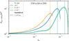 |
Fig. 15 Normalised mean size distribution at the 99th percentile and between 380≤ Ωt ≤ 450 for a dust diffusion factor of α = 0 (run PSI10) in blue, α = 10−8 (run PSIα, 1e−8) in orange, and α = 10−7 (run PSIα, 1e−7) in green. |
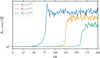 |
Fig. 16 Normalised mean density at the 99th percentile for the different size distributions. Run PSIβ,−3.2 is shown in blue (β = −3.5), run PSI10 in orange, and run PSIβ,−3.8 in green. |
6.4 Dust-to-gas ratio
The SI in the low dust-to-gas ratio regime μ < 1 is a Resonant Drag Instability (RDI) (Squire & Hopkins 2018b), and we can see from Figure A2 in McNally et al. (2021) that there is no substantial growth for the PSI in the low dust-gas-ratio regime (μ = 0.5). This is a direct consequence of the adverse effect of the size distribution on the RDI streaming instability (Paardekooper & Aly (in prep.)). We can compare this to numerical simulations at different dust-to-gas ratios that, if perturbed with white noise, should be able to grow in their fastest-growing mode. This is done with three different dust-gas ratios in runs PSIμ, 3*, PSIμ, 1* and PSIμ, 0.5*, these simulations are perturbed by white noise in the gas, where the standard deviation is 10−4 · cs. When we perturb the gas with white noise, the run at μ = 3 reaches the saturated non-linear regime after Ωt ∼ 75, compared to Ωt ∼ 125 for the standard run (PSI10) where we only perturbed the wavevector K = (30, 0, 30)T. Similar to previous work (e.g. Yang & Zhu 2021; Zhu & Yang 2021; McNally et al. 2021; Krapp et al. 2019), lowering the dust-to-gas ratio will also decrease the growth rate. The run at a dust-to-gas ratio μ = 1 (PSIμ, 1*) takes more than four times as long to reach the saturated non-linear regime at Ωt ∼ 400. However, in contrast to the mSI case, the saturated amplification factor at the 99th percentile has a similar saturated value at μ = 1 as the one of μ = 3, see Figure 18. The normalised size distribution at the 99th percentile of μ = 1 is also very similar to μ = 3, showing the same peaked structure. At a dust-to-gas ratio of μ = 0.5, there is no significant growth of the instability after the full length of the run Ωt =500.
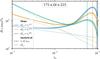 |
Fig. 17 Mean size distribution at the 99th percentile and between 175 ≤ Ωt ≤ 225 for different power law slopes with β = −3.2 (run PSIβ,−3.2) in blue, β = −3.5 (run PSI10) in orange, and β = −3.8 (run PSIβ,−3.8) in green. |
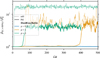 |
Fig. 18 Normalised mean density at the 99th percentile for different dust-to-gas ratios. The figure shows μ = 3 (run PSIμ, 3) in green, μ = 1 (run PSIμ, 1) in orange, and μ = 0.5 (run PSIμ, 0.5) in blue. |
7 Substructure in clumps
The peak in the size distribution at the upper 99th percentile indicates that there is some substructure in clumps. Part of the substructure can be explained by the difference in the density distribution for the different Stokes numbers (Figure 2D). Causing the general trend that the larger Stokes are overrepresented within the 99th percentile of the sum of dust species (the area of 99th percentile contour of the larger Stokes numbers is smaller than the sum of dust and area of the smaller Stokes numbers is larger). This only leads to the overabundance of larger dust sizes in the clumps but does not explain the peak in the size distribution. This is also visible in the dust-size distribution in Figure 9a of Yang & Zhu (2021), where high- μ run (Af) shows an over-representation of the largest dust sizes in the denser regions.
An effect that can lead to the substructure and a peak in the size distribution is a spatial separation between the highestdensity regions of different Stokes. This Stokes-dependent separation can occur through the PSI, where the different dust sizes undergo different drag forces when drifting through the gas. Causing the most decoupled dust sizes (largest Stokes numbers) to be in front of the smaller Stokes sizes in the clumps in the drift direction. We can visualise this by plotting the contour of the densities 99th percentile for the different dust species. This is done for the four largest dust sizes and the sum over all dust species in Figure 19. In this figure, we can see that the individual clumps are made of adjacent filaments of the individual dust species, where we find these filaments are in order of size, with often the largest Stokes number on the left. This corresponds to the direction of the background pressure gradient and drift direction.
The density contour indicates where most of a specific dust is located, but the density and size distribution are more discontinuous. In the numerical simulation, we always need to use a discrete number of dust species (nd = 10 for run PSI101024). Therefore, we see some gaps between the contours. These become smaller if we take the limit to a continuous size distribution (nd → ∞), but the averaged behaviour of the clumps is already converged at nd = 10 (Section 5.2.2). Within a contour of a dust bin, the size distribution is not monodisperse. However, the spatial dispersion in the clumps causes specific regions to be more monodisperse compared to the background distribution.
The spatial separation also causes the peak size distribution in the highest percentiles because the largest Stokes numbers are slightly in front of the rest of the clump, causing part of the dust to fall outside of the percentile contour of the sum of dust species. More of the largest dust species are slightly ahead of the rest of the clump and therefore less present in the densest regions of the sum of the dust species. This showed up in the averaged size distribution at 99th percentile in density as a peak (see Figure 6).
When we take the average size distribution over the contour of individual clumps, we find that the individual clumps also form a peak, and the shape of the size distribution is consistent with the shape of the average size distribution, indicating that the peak is not a symptom of averaging over high-density regions that have different individual compositions.
8 Discussion and conclusion
8.1 Maximum dust density
One of the main results of this paper is that the maximum density of the dust is significantly lower for the PSI than the mSI ∼ O(10); this will make it harder to reach a large enough amplification, where clumping can lead to planetesimal formation. The natural clumping criteria in 3D is the Roche density,
 (32)
(32)
with clumping expected for ρ > ρR. We follow Li & Youdin (2021); Lim et al. (2024b) and apply the same criteria in 2D, but it should be noted that 3D simulations are required to assess clumping using the Roche density. When assuming a low mass disc with a Toomre parameter Q of 32 (Toomre 1964), the Roche density ρR ≈ 180 ρg0. The mSI runs reach the Roche density, but in the PSI simulations we reach a maximum density of ρd, max = 82 ± 14 ρg0 (see run PSI101024 in Figure 2), which would be below the strong clumping criteria of Li & Youdin (2021); Lim et al. (2024b), making it more difficult to form planetesimals through the PSI compared to the mSI. However, since the dust is modelled as a pressureless fluid, a higher spatial resolution will lead to larger densities, possibly exceeding the Roche density.
Another important consideration is that the model we used is simplified in several ways. First of all, we considered only two spatial dimensions. Therefore, the highest-density regions are not true clumps in 3D but are sheets of higher density in 2D. To represent real clumps that could end up becoming planetesimals, we need to consider the 3D simulations; this could affect the shape of the clumps and, in turn, also affect the spatial separation we observe in the highest-density regions between the different dust species.
Secondly, the simulations do not consider self-gravity. This does not prevent us from comparing to clumping criteria; see, for example, Li & Youdin (2021), they studied clumping in 2D simulations without doing self-gravity using the Roche density as criteria. Lim et al. (2024a)7 also shows that switching on selfgravity in 3D simulations of the SI only significantly affects density structure if the maximum density already exceeds the Roche density. Although self-gravity could affect the substructure in the formed clumps, studying the PSI without self-gravity would not significantly change the clumping criteria.
The biggest simplification is that our simulations are unstratified, while previous simulations of the multi-species streaming instability have mostly been stratified 3D simulations (Bai & Stone 2010; Schaffer et al. 2018, 2021; Rucska & Wadsley 2023). Although these simulations show similar trends, such as larger dust species playing a larger role in the formed structure, they cannot directly be compared with the unstratified simulations in this paper or from Yang & Zhu (2021). Lin (2021) shows that the dominant instability in stratified discs is driven by the vertical gradient in the azimuthal velocity of the dusty gas (vertical shear), which provides a source of “free energy” resulting in an instability through partial dust-gas coupling. The vertically shearing streaming instability (VSSI) has fast growth rates compared to the “classical” SI and will likely form the initial turbulence in stratified simulations. Li & Youdin (2021) find that the linear unstratified SI growth rates are not a good predictor for SI clumping in stratified simulations and that analytical growth rates are surprisingly similar to non-clumping runs.
Lastly, the simulations in this paper are isothermal; according to Lehmann & Lin (2023), the non-isothermal SI will suppress sufficiently small-scale modes through radial buoyancy only if the gas cooling timescale is comparable to the dynamical one (β ≈ 1). However, the linear analysis in this paper has been done at larger scale modes (K = 30) and is less affected if we assume the SI occurs in specific regions where the cooling occurs on timescales roughly similar to dynamical. Whether this affects the clumping would have to be tested with non-isothermal simulations.
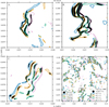 |
Fig. 19 Contour of density at the upper 99th percentile for the sum of the density and the dust bins of the four largest Stokes numbers. The figure shows the substructure of the clumps in the non-linear regime (snapshot at Ωt = 166.5) for the PSI (run PSI101024). |
8.2 Gauss-Legendre integration
We have introduced a new way to implement the integration of the backreaction on the gas, where we take the continuum limit using the GL method to sample the size distribution. We can compare the error in the momentum transfer from the integration (22) in the linear regime, where we found that the GL method converges a lot faster to the continuum limit than the discrete method. The GL method is shown to work well in the linear regime (see Figure 11) where the size distribution is a smooth function, and the momentum transfer integral is wellbehaved and thus can be accurately approximated by the GL nodes. Even though this expectation is no longer valid in the non-linear regime, we notice that the size distribution resulting from the GL integration remains smooth (see Figure 6) and converges with the number of dust species used in the sampling (see Figure 10).
An important distinction is that we take a truly polydisperse approach, that is, with a continuum in sizes, using the GL method. There have also been multi-species SI studies using different numerical integration routines. Bai & Stone (2010) use a particle-fluid approach where the continuous size distribution is discretised into a number of bins with a fixed width in Stokes number in the logarithmic scale (each bin covers half a O(10)), and where equal mass bins are also assumed. A similar method (discrete logarithmic sampling) is used in Krapp et al. (2019); Schaffer et al. (2018); Zhu & Yang (2021); Yang & Zhu (2021). Rucska & Wadsley (2023) also uses equal mass boundaries, but these are not equally spaced linearly or logarithmically. This discrete sampling method is analogous to using a Riemann sum approximation with a midpoint rule and is also bound by the approximation error of this routine. Therefore, at a low number of dust species, this discrete method does not represent the continuous limit, and the integration error between the discrete method and the continuous limit converges significantly slower with the number of dust species than the GL method (see Section 4).
Simulating the PSI using a particle-fluid approach, the dust size distribution can also be quasi-continuously, where each particle is given a unique size sampled from the size distribution. This method is explored in Schaffer et al. (2018, 2021), and is analogous to a Monte-Carlo algorithm for the numerical integration of the momentum transfer, which converges even slower than the midpoint rule.
8.3 Effect on planetesimals
Our analysis revealed that in the densest regions, larger dust sizes are overrepresented, and there is a peak in the size distribution. This peak was not expected, and we explored a couple of explanations, such as the resonant velocity of the size distribution and the spatial separation of the different dust species. The spatial separation is the preferred explanation for the peak in the densest regions, causing the largest dust species to fall outside of the densest region of the sum over all the dust. The observed size distribution in these densest regions can mimic the distribution that can result from dust growth (Birnstiel et al. 2011). We can form the peak in the sized distribution through dynamics and the size-dependent coupling between the gas and the dust, without dust growth or fragmentation. That the size distribution changes through dynamics can in turn also affect coagulation, by e.g. making the size distribution locally more monodisperse. Therefore, combining coagulation with polydisperse hydrodynamical simulations of the SI would be an important further step.
If the peak in the size distribution persists when the density exceeds the Roche density, the peak in the size distribution also ends up in rubble pile asteroids (Chapman 1978; Walsh 2018; Visser et al. 2021). The size distribution of the particles making up the rubble pile can be observed (e.g. Gundlach & Blum 2013; Blum et al. 2017; Fulle & Blum 2017). The observed size distribution can then inturn be an indication of the formation history and the local environment where the asteroid was formed through gravitational collapse, taking into account how the PSI changes the size distribution in the highest-density regions. However, we then need to consider that the size of the aggregates can change during the collapse (Wahlberg Jansson & Johansen 2017; Pinto et al. 2021; Visser et al. 2021), although the size distribution at the Roche density can also affect the cloud collapse. The size distribution can also change at later stages due to radiative or chemical reactions or kinetic impacts (Poulet et al. 2016; Graves et al. 2019; Hsu et al. 2022). Although this primarily affects the surface, the interior of the asteroid, below a layer of a few tens of centimetres, can still represent the primordial size distribution (Capria et al. 2017).
8.4 Summary
We investigate the 2D unstratified PSI using FARGO3D, focusing on the evolution of the continuous size distribution and morphology in the densest dust structures. The main results and findings of this paper are as follows:
The Gauss-Legendre quadrature method used for sampling the size distribution converges much faster with the number of dust species compared to a discrete method when we compared the growth rates of the numerical simulations to the analytical growth rate (see Section 4). This allowed us to use fewer dust species whilst maintaining an acceptable accuracy on the momentum transfer between the dust and the gas in the continuum limit, which can be significantly less computationally expensive.
Similar to previous work (Krapp et al. 2019; Paardekooper et al. 2020, 2021; McNally et al. 2021; Zhu & Yang 2021), we find that the PSI has slower growth rates than the mSI. This makes the parameter space where the PSI can be triggered to form clumps smaller, especially when considering that the growth rate of the PSI changes faster with a maximum Stokes number or dust diffusion than the mSI (see Section 4 and 6.1 for more details).
In the regimes where the PSI forms clumps, the amplification factor can be up to an order of ten smaller than the mSI at the maximum Stokes number of the PSI range, making it more difficult for the clumps to reach the Roche density limit and collapse into planetesimals.
The PSI cannot be represented by an mSI run with properties that are derived from the averaged properties of the PSI setup such as average Stokes number and total dust density of the size distribution, and the PSI is not a simple summation of individual discrete mSI cases at different Stokes numbers.
There is a correlation between the location of higher density regions of the different dust sizes in a PSI run, although the larger dust sizes clump more. There is a pronounced overrepresentation of larger dust species in the dense regions in the non-linear regime. This overrepresentation occurs because smaller dust particles are more tightly coupled to the nearly incompressible gas, which limits their ability to clump as effectively as the larger dust species.
We observed a peak in the size distribution of the densest regions. This peak arises from the spatial segregation of the differently sized dust species, where particles with the largest Stokes numbers are located just outside the densest areas of the total dust density (the combined dust species). This spatial separation plays a crucial role in shaping the size distribution in these regions.
The peak in the size distribution at the densest regions can mimic the distribution we observed when we had dust growth (Birnstiel et al. 2011). We find that through dynamics and size-dependent coupling between the gas and dust, we can form a size distribution with a bump on top of the background MRN distribution without dust growth or fragmentation.
Our findings highlight that it is more difficult to form planetesimals considering the more realistic polydisperse case. In the PSI we find distinct features in the densest regions. To consider a more realistic comparison to clumping that leads to planetesimal formation, future work should consider the 3D stratifield setup.
Data availability
The data that support the findings of this study are openly available in 4TU.ResearchData under the name: Data underlying the manuscript “Polydisperse Formation of Planetesimals” at http://doi.org/10.4121/8f0a99b2-7d55-4e05-aa8f-345cab38ff38. The code that processes the output of FARGO3D and supports the findings of this study is openly available in 4TU.ResearchData under the name: Code underlying the manuscript “Polydisperse Formation of Planetesimals” at http://doi.org/10.4121/528086f3-b288-482f-ab45-3c5ccb18a293.
Acknowledgements
We would like to thank the anonymous referee for their invaluable feedback. We would like to thank Benjamin Silk and Tom Konijn for their useful comments. This project has received funding from the European Research Council (ERC) under the European Union's Horizon Europe research and innovation programme (Grant Agreement No. 101054502). The authors acknowledge the use of computational resources of the DelftBlue supercomputer, provided by Delft High Performance Computing Centre (DHPC). This work made use of several open-source software packages. We acknowledge numpy (Harris et al. 2020), matplotlib (Hunter 2007), scipy (Virtanen et al. 2020), FARGO3D (Benítez-Llambay & Masset 2016; BenítezLlambay et al. 2019), and psitools (Paardekooper et al. 2020, 2021; McNally et al. 2021). We acknowledge 4TU. ResearchData for supporting open access to research data.
References
- Bai, X.-N., & Stone, J. M. 2010, ApJ, 722, 1437 [NASA ADS] [CrossRef] [Google Scholar]
- Benítez-Llambay, P., & Masset, F. S. 2016, ApJS, 223, 11 [Google Scholar]
- Benítez-Llambay, P., Krapp, L., & Pessah, M. E. 2019, ApJS, 241, 25 [Google Scholar]
- Birnstiel, T., Ormel, C. W., & Dullemond, C. P. 2011, A&A, 525, A11 [NASA ADS] [CrossRef] [EDP Sciences] [Google Scholar]
- Blum, J., Gundlach, B., Krause, M., et al. 2017, MNRAS, 469, S755 [Google Scholar]
- Capria, M. T., Capaccioni, F., Filacchione, G., et al. 2017, MNRAS, 469, S685 [Google Scholar]
- Chapman, C. R. 1978, NASA Conf. Publ., 2053, 145 [Google Scholar]
- Chen, K., & Lin, M.-K. 2020, ApJ, 891, 132 [Google Scholar]
- Delft High Performance Computing Centre (DHPC). 2024, DelftBlue Supercomputer (Phase 2), https://www.tudelft.nl/dhpc/ark:/44463/DelftBluePhase2 [Google Scholar]
- Draine, B. T., & Lee, H. M. 1984, ApJ, 285, 89 [NASA ADS] [CrossRef] [Google Scholar]
- Epstein, P. S. 1924, Phys. Rev., 23, 710 [Google Scholar]
- Fulle, M., & Blum, J. 2017, MNRAS, 469, S39 [NASA ADS] [CrossRef] [Google Scholar]
- Garaud, P., Barrière-Fouchet, L., & Lin, D. N. C. 2004, ApJ, 603, 292 [NASA ADS] [CrossRef] [Google Scholar]
- Goldreich, P., & Lynden-Bell, D. 1965, MNRAS, 130, 125 [Google Scholar]
- Graves, K. J., Minton, D. A., Molaro, J. L., & Hirabayashi, M. 2019, Icarus, 322, 1 [NASA ADS] [CrossRef] [Google Scholar]
- Gundlach, B., & Blum, J. 2013, Icarus, 223, 479 [Google Scholar]
- Harris, C. R., Millman, K. J., van der Walt, S. J., et al. 2020, Nature, 585, 357 [NASA ADS] [CrossRef] [Google Scholar]
- Hsu, H.-W., Wang, X., Carroll, A., Hood, N., & Horányi, M. 2022, Nat. Astron., 6, 1043 [NASA ADS] [CrossRef] [Google Scholar]
- Hunter, J. D. 2007, Comput. Sci. Eng., 9, 90 [NASA ADS] [CrossRef] [Google Scholar]
- Jacquet, E., Balbus, S., & Latter, H. 2011, MNRAS, 415, 3591 [NASA ADS] [CrossRef] [Google Scholar]
- Johansen, A., Oishi, J. S., Mac Low, M.-M., et al. 2007, Nature, 448, 1022 [Google Scholar]
- Krapp, L., Benítez-Llambay, P., Gressel, O., & Pessah, M. E. 2019, ApJ, 878, L30 [Google Scholar]
- Lehmann, M., & Lin, M.-K. 2023, MNRAS, 522, 5892 [CrossRef] [Google Scholar]
- Li, R., & Youdin, A. N. 2021, ApJ, 919, 107 [NASA ADS] [CrossRef] [Google Scholar]
- Lim, J., Simon, J. B., Li, R., et al. 2024a, ApJ, 969, 130 [NASA ADS] [CrossRef] [Google Scholar]
- Lim, J., Simon, J. B., Li, R., et al. 2024b, arXiv e-prints [arXiv:2410.17319] [Google Scholar]
- Lin, M.-K. 2021, Apj, 907, 64 [NASA ADS] [CrossRef] [Google Scholar]
- Magnan, N., Heinemann, T., & Latter, H. N. 2024, MNRAS, 529, 688 [NASA ADS] [CrossRef] [Google Scholar]
- Mathis, J. S., Rumpl, W., & Nordsieck, K. H. 1977, ApJ, 217, 425 [Google Scholar]
- McNally, C. P., Lovascio, F., & Paardekooper, S.-J. 2021, MNRAS, 502, 1469 [NASA ADS] [CrossRef] [Google Scholar]
- Mottola, S., Arnold, G., Grothues, H. G., et al. 2015, Science, 349, 2.232 [NASA ADS] [CrossRef] [Google Scholar]
- Nakagawa, Y., Sekiya, M., & Hayashi, C. 1986, Icarus, 67, 375 [Google Scholar]
- Nesvorný, D., Li, R., Youdin, A. N., Simon, J. B., & Grundy, W. M. 2019, Nat. Astron., 3, 808 [CrossRef] [Google Scholar]
- Paardekooper, S.-J., McNally, C. P., & Lovascio, F. 2020, MNRAS, 499, 4223 [CrossRef] [Google Scholar]
- Paardekooper, S.-J., McNally, C. P., & Lovascio, F. 2021, MNRAS, 502, 1579 [NASA ADS] [CrossRef] [Google Scholar]
- Pinto, G. A., Marrocchi, Y., Morbidelli, A., et al. 2021, ApJ, 917, L25 [CrossRef] [Google Scholar]
- Poulet, F., Lucchetti, A., Bibring, J. P., et al. 2016, MNRAS, 462, S23 [Google Scholar]
- Rucska, J. J., & Wadsley, J. W. 2023, MNRAS, 526, 1757 [NASA ADS] [CrossRef] [Google Scholar]
- Schäfer, U., Johansen, A., & Banerjee, R. 2020, A&A, 635, A190 [Google Scholar]
- Schaffer, N., Yang, C.-C., & Johansen, A. 2018, A&A, 618, A75 [NASA ADS] [CrossRef] [EDP Sciences] [Google Scholar]
- Schaffer, N., Johansen, A., & Lambrechts, M. 2021, A&A, 653, A14 [NASA ADS] [CrossRef] [EDP Sciences] [Google Scholar]
- Shakura, N. I., & Sunyaev, R. A. 1973, A&A, 24, 337 [NASA ADS] [Google Scholar]
- Simon, J. I., Cuzzi, J. N., McCain, K. A., et al. 2018, Earth Planet. Sci. Lett., 494, 69 [CrossRef] [Google Scholar]
- Simon, J. B., Blum, J., Birnstiel, T., & Nesvorný, D. 2022, arXiv e-prints [arXiv:2212.04509] [Google Scholar]
- Squire, J., & Hopkins, P. F. 2018a, MNRAS, 477, 5011 [Google Scholar]
- Squire, J., & Hopkins, P. F. 2018b, ApJ, 856, L15 [NASA ADS] [CrossRef] [Google Scholar]
- Squire, J., & Hopkins, P. F. 2020, MNRAS, 498, 1239 [NASA ADS] [CrossRef] [Google Scholar]
- Tanaka, H., Himeno, Y., & Ida, S. 2005, ApJ, 625, 414 [NASA ADS] [CrossRef] [Google Scholar]
- Toomre, A. 1964, ApJ, 139, 1217 [Google Scholar]
- Umurhan, O. M., Estrada, P. R., & Cuzzi, J. N. 2020, ApJ, 895, 4 [Google Scholar]
- Virtanen, P., Gommers, R., Oliphant, T. E., et al. 2020, Nat. Methods, 17, 261 [Google Scholar]
- Visser, R. G., Drążkowska, J., & Dominik, C. 2021, A&A, 647, A126 [NASA ADS] [CrossRef] [EDP Sciences] [Google Scholar]
- Wahlberg Jansson, K., & Johansen, A. 2017, MNRAS, 469, S149 [Google Scholar]
- Walsh, K. J. 2018, ARA&A, 56, 593 [NASA ADS] [CrossRef] [Google Scholar]
- Weber, P., Pérez, S., Benítez-Llambay, P., et al. 2019, ApJ, 884, 178 [NASA ADS] [CrossRef] [Google Scholar]
- Weidenschilling, S. J. 1977, Ap&SS, 51, 153 [Google Scholar]
- Yang, C.-C., & Zhu, Z. 2021, MNRAS, 508, 5538 [NASA ADS] [CrossRef] [Google Scholar]
- Yang, C.-C., Mac Low, M.-M., & Johansen, A. 2018, ApJ, 868, 27 [NASA ADS] [CrossRef] [Google Scholar]
- Youdin, A. N., & Goodman, J. 2005, ApJ, 620, 459 [Google Scholar]
- Youdin, A., & Johansen, A. 2007, ApJ, 662, 613 [Google Scholar]
- Zhu, Z., & Yang, C.-C. 2021, MNRAS, 501, 467 [Google Scholar]
This will be further explored in Paardekooper and Aly (in prep.), where the authors show that the RDI streaming instability is particularly negatively affected by the size distribution.
See for example, the difference between model Af (the fast-growing instability, run with μ = 2 and in the high −μ SI regime) and As (the slow instability with μ = 0.2) in Yang & Zhu (2021).
We note that we use a dimensional pressure support parameter η similar to Paardekooper et al. (2020, 2021); McNally et al. (2021). This parameter is related to the non-dimensional parameter defined in Youdin & Goodman (2005) by η = r0 Ω2 ηYG. This is a largely cosmetic choice allowing us to use a length scale of η/Ω2, without using r0 the orbital radius of the shearing box.
Except the simulations of varying dust-to-gas ratio, these are perturbed with white noise in the gas, with a standard deviation of 10−4cs.
In the mSI runs, we observe a numerical artefact in the gas density on the scale of the grid cells, the PSI is unaffected. A similar error in the mSI is also mentioned in Section 3.5.5 of Benítez-Llambay et al. (2019).
Section 3.2.
All Tables
All Figures
|
Fig. 1 Integration of a normalised log-normal distribution (dashed line) using a discrete method (blue line) and a Gauss-Legendre quadrature (orange line). |
| In the text | |
|
Fig. 2 Time evolution of the mSI (run: mSI1024) and PSI (run: PSI101024). The dot-dashed line shows the mSI run, the solid lines show the ten individual dust species of the PSI run, and the dotted line is the sum over all the dust species. Plot A shows the amplitude of the largest mode in the shearing box (A sinusoid with wavenumber K = (30, 0, 30)T), plot B shows the maximum density in the shearing box, plot C shows the mean density at every snapshot's 99th percentile and plot D shows the average probability density function of the normalised density distribution in the non-linear regime between (140 ≤ Ωt ≤ 160). |
| In the text | |
|
Fig. 3 Normalised amplitude of the largest mode of the shearing box (a sinusoid with a wavenumber K=(30, 0, 30)T) for different numbers of dust species and sampling methods. The runs with ten dust species are shown in blue, 20 dust species are shown in orange, and 40 dust species are shown in green. The solid line indicates the GL method (27), and the dotted line indicates a log-linear sampling method (runs: PSI20, PSI10, PSI40disc., PSI20disc., and PSI10disc..). The dot-dashed line is an analytical solution of the growth rate calculated with psitools. |
| In the text | |
|
Fig. 4 Efficientcy of dust compression as a function of Stokes number. The top plot shows the growth rate in the linear regime at wavevector K = (30, 0, 30)T for setups with different maximum Stokes numbers τs, max. The solid orange and blue lines are the analytical growth rates (for mSI and PSI, respectfully) calculated with psitools (McNally et al. 2021). The diamonds indicate the fitted values of the growth rate in the linear regime of the numerical simulations. In the bottom plot, the diamonds correspond to the fitted values of the saturated amplification factor of the maximum density in the non-linear regime. The solid grey lines indicate the values for run PSI10, and the dotted grey line indicates the average Stokes number of the size distribution of run PSI10. |
| In the text | |
|
Fig. 5 Snapshot of the normalised density in the non-linear regime (Ωt = 166) for the PSI run PSI101024. The figure shows the density of the sum of the dust species (upper left), gas (lower left), and nine of the ten individual dust species with an increasing Stokes number.) |
| In the text | |
|
Fig. 6 Top: mean size distribution in the 99th percentile at different times. The dotted line indicates the size distribution at Ωt = 0. Bottom: same size distribution normalised by the background-size distribution σ0(τs). The dashed line indicates the Stokes number corresponding to the resonant velocity, and the dot-dashed line is the average Stokes number of the size distribution at Ωt = 0. |
| In the text | |
|
Fig. 7 Normalised (mean) density at the densest pixel and at the 99th percentile (indicated by darker and lighter colours; respectively) for different spatial resolutions. The mSI runs at different resolutions are indicated with the dotted line for run mSI1024, mSI512, and mSI using green, orange, and blue, respectively. The PSI runs PSI101024, PSI10512, and PSI10 have the same colour coding as the mSI runs. |
| In the text | |
|
Fig. 8 Normalised mean size distribution at the 99th and 90th percentiles and between 140 ≤ Ωt ≤ 160 using the same PSI runs and colour scheme as Figure 7. |
| In the text | |
|
Fig. 9 Normalised mean density at the 99th percentile for different numbers of dust species from run mSI1024 (indicated with a dotted pink line), run PSI511024 (in blue), run PSI101024 (in orange), and run PSI201024 (in green). |
| In the text | |
|
Fig. 10 Normalised mean size distribution at the 99th percentile and between 135 ≤ Ωt ≤ 145 using the same PSI runs and colour scheme as Figure 9. The dashed line indicates the Stokes number at resonance velocity |
| In the text | |
|
Fig. 11 Normalised mean size distribution at the 99th percentile and between 150 ≤ Ωt ≤ 200. The top plot shows the PSI run with ten dust species sampled from the GL in blue (run PSI10) and the PSI run with ten dust species uniformly sampled from a logarithmic scale in green (run PSI10disc.), and the bottom plot shows the PSI run using 20 dust species sampled from the GL in orange (run PSI20) and the PSI run with 20 dust species uniformly sampled from a logarithmic scale in pink (run PSI2 θdisc.). |
| In the text | |
|
Fig. 12 Time evolution of the mSI (runs: [mSI*, mSIα,1e−8, mSIα,1e−7, mSIα,1e−6]) are shown with dotted lines and PSI (runs: [PSI*, PSIα, 1e−8, PSIα,1e−7, PSIα, 1e−6]) are shown with solid lines for different dust diffusion coefficients α. The colour indicates the diffusion coefficient, where no diffusion is shown in blue, α = 10−8 in orange, α = 10−7 in green, and α = 10−8 in pink. The top plot shows the amplitude of the largest mode in the shearing box (A sinusoid with wavenumber Kx,z = 30), and the dashed lines and dash-dotted lines show the analytical results calculated with psitools for the corresponding α. The bottom plot shows the normalised mean density at the 99th percentile for every snapshot. |
| In the text | |
|
Fig. 13 Normalised mean size distribution at the 99th percentile and between 380 ≤ Ωt ≤ 450 for a dust diffusion coefficient of α = 0 (run PSI1Q) in blue, α = 10−8 (run PSIα,1e−8) in orange, and α = 10−7 (run PSIα,1e−7) in green. |
| In the text | |
|
Fig. 14 Time evolution of the mSI (runs: [mSI*, mSIτs,5e−2, mSIτs,2e−1]) are shown with a dotted lines and PSI (runs: [PSI*, PSIτs,5e−2, PSIτs,2e−1]) are shown with solid lines for different peak Stokes numbers τs,max. The colour indicates maximum Stokes Number with τs = 0.05 in blue, τs = 0.1 in orange, and τs = 0.2 in green. The top plot shows the amplitude of the largest mode in the shearing box (A sinusoid with wavenumber Kx,z = 30), and the dashed lines and dash-dotted lines show the analytical results calculated with psitools for the corresponding α. The bottom plot shows the normalised mean density at the 99th percentile for every snapshot. |
| In the text | |
|
Fig. 15 Normalised mean size distribution at the 99th percentile and between 380≤ Ωt ≤ 450 for a dust diffusion factor of α = 0 (run PSI10) in blue, α = 10−8 (run PSIα, 1e−8) in orange, and α = 10−7 (run PSIα, 1e−7) in green. |
| In the text | |
|
Fig. 16 Normalised mean density at the 99th percentile for the different size distributions. Run PSIβ,−3.2 is shown in blue (β = −3.5), run PSI10 in orange, and run PSIβ,−3.8 in green. |
| In the text | |
|
Fig. 17 Mean size distribution at the 99th percentile and between 175 ≤ Ωt ≤ 225 for different power law slopes with β = −3.2 (run PSIβ,−3.2) in blue, β = −3.5 (run PSI10) in orange, and β = −3.8 (run PSIβ,−3.8) in green. |
| In the text | |
|
Fig. 18 Normalised mean density at the 99th percentile for different dust-to-gas ratios. The figure shows μ = 3 (run PSIμ, 3) in green, μ = 1 (run PSIμ, 1) in orange, and μ = 0.5 (run PSIμ, 0.5) in blue. |
| In the text | |
|
Fig. 19 Contour of density at the upper 99th percentile for the sum of the density and the dust bins of the four largest Stokes numbers. The figure shows the substructure of the clumps in the non-linear regime (snapshot at Ωt = 166.5) for the PSI (run PSI101024). |
| In the text | |
Current usage metrics show cumulative count of Article Views (full-text article views including HTML views, PDF and ePub downloads, according to the available data) and Abstracts Views on Vision4Press platform.
Data correspond to usage on the plateform after 2015. The current usage metrics is available 48-96 hours after online publication and is updated daily on week days.
Initial download of the metrics may take a while.