| Issue |
A&A
Volume 695, March 2025
|
|
|---|---|---|
| Article Number | A105 | |
| Number of page(s) | 11 | |
| Section | The Sun and the Heliosphere | |
| DOI | https://doi.org/10.1051/0004-6361/202452638 | |
| Published online | 11 March 2025 | |
Spatial and temporal super-resolution methods for high-fidelity solar imaging
1
Taras Shevchenko National University of Kyiv, Glushkova Ave., 4, 03127 Kyiv, Ukraine
2
Department of Physics, The Chinese University of Hong Kong, Hong Kong
3
Center for Computation Astrophysics, Flatiron Institute, New York, NY 10010, USA
4
Department of Astrophysical Sciences, Princeton University, 4 Ivy Lane, Princeton, NJ 08544, USA
5
Department of Physics & Center for Data Science, New York University, 726 Broadway, New York, NY 10003, USA
⋆ Corresponding author; This email address is being protected from spambots. You need JavaScript enabled to view it.
Received:
16
October
2024
Accepted:
22
January
2025
Abstract
Context. The Sun plays a significant role in space weather by emitting energy and electromagnetic radiation that influence the environment around the Earth. Missions such as SOHO, STEREO, and SDO captured solar observations at multiple wavelengths to monitor and predict solar events. However, the data transmission from these missions is often constrained, in particular, for those operating at greater distances from Earth. This limits the availability of continuous observations.
Aims. We increase the spatial and temporal resolution of solar images to improve the quality and availability of solar data. By addressing telemetry constraints and providing more detailed solar image reconstructions, we seek to facilitate a more accurate analysis of solar dynamics and improve space weather prediction.
Methods. We applied deep-learning techniques, specifically, a UNet-based architecture, to generate high-resolution solar images that enhance the intricate details of the solar structures. Additionally, we used a similar architecture to reconstruct solar image sequences with a reduced temporal resolution to predict missing frames and restore temporal continuity.
Results. Our deep-learning approach successfully enhances the resolution of solar images and reveals finer details of solar structures. The model also predicts missing frames in solar image sequences, which allows more continuous observation despite telemetry constraints. These advancements contribute to a better analysis of solar dynamics and set the stage for an improved space weather forecasting and future solar physics research.
Key words: methods: data analysis / Sun: activity / Sun: atmosphere
© The Authors 2025
 Open Access article, published by EDP Sciences, under the terms of the Creative Commons Attribution License (https://creativecommons.org/licenses/by/4.0), which permits unrestricted use, distribution, and reproduction in any medium, provided the original work is properly cited.
This article is published in open access under the Subscribe to Open model. This email address is being protected from spambots. You need JavaScript enabled to view it. to support open access publication.
1. Introduction
As the central star of our Solar System, the Sun plays an important role in shaping our understanding of cosmic dynamics and their impact on Earth. To study its complex surface features, such as dynamic solar flares or subtle variations in radiation, we clearly need high-resolution images. While advancements in spatial resolution have been achieved through both space-based (Pesnell et al. 2012a) and ground-based (Rimmele et al. 2020) telescopes, they come at significant cost in terms of manufacturing and maintenance. Ground-based telescopes also face the challenge of atmospheric turbulence, which can degrade the image clarity (Cai et al. 2023). An improved spatial resolution not only enhances individual images, but also facilitates the integration of data from diverse instruments, especially when information from sources with varying resolutions is combined. Super-resolution methods based on neural networks play a key role in standardizing the resolution across datasets by optimizing the subsequent analysis and integration better than known mechanisms such as interpolation. Higher-resolution images are also valuable for various computer vision tasks, where they provide much-needed detail for an accurate analysis of solar events (Hanslmeier & Messerotti 1999). For example, in solar event detection and anomaly tracking, high-resolution inputs improve the precision of analytical and detection algorithms. Beyond a machine-based analysis, human observers benefit from clearer images, particularly in fields in which visual interpretation is important, such as educational materials or public outreach. Therefore, it is essential to develop a comprehensive model for increasing the spatial resolution of solar images to advance scientific research.
Furthermore, to better understand solar phenomena and predict solar events, space missions such as the Solar Heliospheric Observatory (SOHO) (Domingo et al. 1995), the Solar Terrestrial Relations Observatory (STEREO) (Kaiser et al. 2008), and the Solar Dynamics Observatory (SDO) (Pesnell et al. 2012b) collect data across various wavelengths, including ultraviolet (UV), extreme-ultraviolet (EUV), magnetograms, and dopplergrams. These datasets allow researchers to study the solar magnetic field and anticipate events such as solar flares and coronal mass ejections (CMEs), which are vital for space weather forecasting. However, space missions often face constraints due to limitations in the data transmission from satellites to Earth. For missions like STEREO (Kaiser et al. 2008), which operates in a solar orbit, the signal strength can be severely impacted during solar conjunction, which results in a reduced data availability, with transmission cadences ranging from five minutes to two hours (Therese 2015). Efforts to address this issue have included synthesizing EUV images from other wavelengths and reducing the data transmission requirements of space missions (Salvatelli et al. 2019).
In this paper, we propose a neural network based on the UNet architecture (Ronneberger et al. 2015) that is designed to enhance the resolution of solar images from sizes of 642, 1282, and 2562 up to 10242. Additionally, we present a deep-learning approach using the UNet model for solar image-sequence reconstruction. Our method predicts missing frames within a sequence of solar images, given the first and last frames. By using deep neural networks, we aim to restore the temporal resolution of solar image data, thereby improving the analysis of solar dynamics over time and mitigating telemetry constraints for future missions operating further from Earth.
2. Machine-learning models
To achieve the goal of super-resolving low-resolution solar images in both time and space, we chose the UNet architecture for its proven effectiveness in image enhancement tasks (Ronneberger et al. 2015). It consists of pairs of two consistent convolutional blocks with skip connections between each stage and a bottleneck, that is, two consistent convolutional blocks without a pair. The model then attempts to generate the desired images along the expansion path. The generated images are pixel-wise compared with the target images, and the gradient is backpropagated through the loss function. The architecture of the model for temporal super-resolution is shown in Figure 1. A similar architecture is also used in spatial super-resolution, but with only three pairs of double convolutional blocks, and a dropout rate of 0.25 is introduced at each convolutional layer.
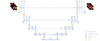 |
Fig. 1. UNet-based architecture used for the temporal reconstruction of solar images, where n represents the input length of the solar image sequence. Each box corresponds to a multichannel feature map. The gray boxes are copied maps. The number of channels is shown at the top of the box. The resolution in pixels is indicated at the side of the box. The arrows represent operations. A similar architecture is also used in spatial super-resolution, but with only three pairs of double convolutional blocks, and a dropout rate of 0.25 is introduced at each convolutional layer. |
For the spatial super-resolution, the model consisted of two pairs of two consistent convolutional blocks and one block without a pair (three-layer UNet). The input to the model consisted of downsized cutouts of solar images at 171 Å, with dimensions of 642, 1282, and 2562 pixels, respectively. Three different models were trained, corresponding to different input resolutions. The goal of the model was to predict the original cutouts of solar images with dimensions of 10242 pixels.
For the temporal reconstruction, the model consisted of three pairs of two consistent convolutional blocks and one block without a pair (four-layer UNet). The input to the model consisted of a series of consecutive solar images taken at hourly intervals with length n, and the middle images were masked and replaced by the linearly interpolated images Ii between the first and last images,
 (1)
(1)
where n is the total number of images, and i is the index of images ranging from 1 to n − 1. By using skip connections, the network started with this basic linearly interpolated version. The goal of the model was to produce interpolations that are better aligned with the ground images. Nine different models were trained, corresponding to nine different passbands captured in SDO.
It is worth noting that generative adversarial networks (GANs) (Goodfellow et al. 2014) are commonly used to enhance the image contrast in image-to-image translation tasks for solar data (Dash et al. 2022). However, since our reference images are from the same observation, it was sufficient to use the mean squared error (MSE) as the loss function to produce high-contrast images. This approach also avoids the potential issue of mode collapse, which can occur in GAN-based methods.
3. Data description and preprocessing
Our work is based on data from the instrument on board the SDO (Pesnell et al. 2012a): the Atmospheric Imaging Assembly (AIA) (Lemen et al. 2011). The AIA instrument captures full-disk solar observations with 4096 by 4096 pixels. It provides observations of the photosphere, chromosphere, and corona in two ultraviolet (UV) passbands every 24 seconds and in seven extreme-ultraviolet (EUV) passbands every 12 seconds.
To achieve spatial super-resolution, we created a dataset consisting of cutouts of AIA images from the Solar Dynamics Observatory (SDO) at the 171 Å passband using version 5.0.1 of the SunPy open-source software package (Mumford et al. 2023). The cutouts were obtained at 12-hour intervals from January 2011 to January 2019. The dataset comprised a total of 5700 datapoints, that is, 5224 training and 581 validation images, which were processed into three-dimensional tensors, corrected for optical degradation, and normalized by exposure time. Images of originally 64 × 64, 128 × 128, and 256 × 256 were resized to 1024 × 1024 using bicubic interpolation to ensure consistent comparisons during the evaluation stage and to use it as a baseline model.
For the temporal reconstruction, we used a curated dataset called SDOML (Galvez et al. 2019). SDOML is a subset of the original SDO data from 2010 to 2018, covering the majority of solar cycle 24. After selecting data with scientific quality, we normalized them by exposure time and corrected them for instrument degradation, with the solar disk size fixed at 976 arcsec. Their temporal and spatial resolutions were down-sampled into 6 minutes and 512 by 512 pixels, respectively, with a pixel size of 4.8 arcsec.
To simulate the data availability in situations with reduced telemetry rates like for the STEREO, we further temporally subselected the images to a cadence of one hour. As a result, we obtained a total of 60 623 samples at each passband (a total of 545 661 images). We divided our datasets into training, validation, and test sets in chronological order. For each passband, we selected 7716 samples from 2011 as the validation dataset, 47 780 samples from 2012 to 2017 as the training dataset, and the remaining 5127 samples from 2018 as the evaluation dataset. This enabled us to evaluate the model performance on images with possible shifted behaviors over the solar cycle.
4. Results and discussion
In this section, we present a comprehensive evaluation of our model performance on spatial and temporal super-resolution tasks. To ensure that we evaluated everything properly, we used different methods and measurements, such as the Pearson correlation coefficient (PCC), relative error (RE), the structural similarity index measure (SSIM), and the percentage of pixel error (PPE). Additionally, we implemented more complex methods, including performing a fast Fourier transform (FFT) on the entire test set to analyze the model performance in the frequency domain. For better visualization and interpretability of the results, we also included histograms and scatterplots to highlight key patterns and relations.
4.1. Evaluation metrics
To quantify our results, we calculated four types of metrics between the SDO/AIA images and the generated images across the entire evaluation dataset. Additionally, we focused exclusively on pixels within the solar disk because they contain the most significant features for evaluating the temporal reconstruction model. This was achieved by cropping the images to a fixed disk size, as specified in the dataset.
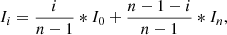
The first metric for the evaluation was the pixel-to-pixel PCC, which was calculated as
 (2)
(2)
where xi, yi in case of RGB images was expanded to (xi1, yi1),(xi2, yi2),(xi3, yi3), corresponding to the R, G, and B color channels, and n is the total number of samples in the validation set. A higher value of the PCC indicates that the model is not only able to generate the correct pixel values, but also that the values are spatially correct.
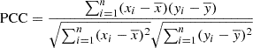
The second metric for the evaluation was the average relative error (RE) of the total pixel value yi, which is given by
 (3)
(3)
where  and yi represent the total pixel values of the generated image and the ground-truth image, respectively, and n is the total number of samples in the validation set. A lower absolute value of the RE indicates a better performance of the model.
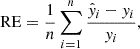
The third metric for the evaluation was the percentage of pixels with REs lower than 10% (PPE10). A higher value of PPE10 indicates more good pixels in the generated images.
The forth metric for the evaluation was the structural similarity index measure (SSIM) (Wang et al. 2004). It can qualify the similarity between two images by modeling the perceived change in the structural image information. A higher value of the SSIM indicates that the structure of the image is well preserved.
All the metrics were calculated for both approaches and all the models. They are shown and discussed in the next subsections.
4.2. Spatial super-resolution
As stated, we obtained three models trained on different resolutions. To analyze the results, we first compared them visually. Figure 2 shows an image with an intensive and highly heterogeneous structure. The 642 resolution model successfully defined relatively small regions and separated them as in the high-quality image. All the models also highlighted regions of minimum and maximum intensity, which facilitates a visual analysis of the image. On the other hand, weaker regions remain smoother than in the high-resolution image. A substantial body of work therefore remains to be addressed.
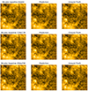 |
Fig. 2. Comparative performance plot across various models. From top to bottom, the rows delineate three distinct models characterized by progressively higher resolution inputs. From left to right, the columns depict the input image, prediction, and ground truth, respectively. |
We then performed some more qualitative comparisons. First of all, we examined the power spectrum and transfer function from Jindal et al. (2023) of the obtained model predictions. The results of this analysis are shown in Figure 3. At lower frequencies, the difference between the ground truth, the predictions, and the input data is minimal because the background frequencies are not significantly altered when the resolution of the images is reduced. The most notable differences arise at higher frequencies, which correspond to the finer details of the images. In these cases, all three models show significant improvements.
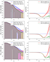 |
Fig. 3. Power spectra and transfer function fractional errors (TFFE) for all three models. The solid, dotted, and dashed lines in the left column represent average power spectra for the whole test set (target, input, and prediction, respectively). The shading around the lines shows the sigma ranges. In the right column, the solid line represents the average TFFE for the prediction and the target, and the dashed line represents the same for the baseline and the target. This time, the shading represents the functional errors through partial derivatives. |
Figure 4 shows the comparison between the input low-resolution image (2562 resolution), shown in the left panel, and the predicted image in the middle with the 10242 resolution. The right panel shows the pixel-wise difference between the ground truth and the resulting image. Higher intensities (pixel values) are represented by brighter colors. This image was chosen randomly from the test data and clearly shows that the difference is higher in dimmer regions, while the difference between brighter regions oscillates near zero values. Because brighter regions change significantly more clearly, the solar activity also becomes more defined and visually divided from the calm zones.
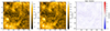 |
Fig. 4. Comparison between the input low-resolution image (2562 resolution), shown in the left panel, and the predicted image in the middle (10242 resolution). The third panel shows the pixel-wise difference between the ground truth and the resulting image. A larger difference corresponds to higher values in the residual plot (the hotter color of the color map). The model performs better in more intensive regions. |
Figure 5 shows difference plots for two different models. The top image in the left panel represents a pixel-to-pixel comparison between the predicted image and the ground truth for the x64 model, but only for pixel values in the μ + 3σ interval. Thereafter, the bottom left plot shows the difference between prediction and ground truth, but only values beyond the μ + 3σ interval. The number of outliers is around 3%. These plots were made to show that the net performs greatly on average, but in the outlier regions (dimmer zones), the difference becomes significantly higher. The right panel shows the same dependence, but for the x256 model. This was done to perform a better visual comparison between the models in the case of the pixel-to-pixel comparison. The pixel difference values for the x256 model are much lower than for the x64 model. The local differences are weaker than for x64, so that the model performed more stably in terms of the difference results. For the x256 case, Figure 9 shows the distribution of the pixel values for the difference between the ground truth and the prediction for the same image as in Figure 4.
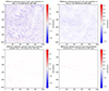 |
Fig. 5. Pair of columns depicting various data representations. The top left panel shows the disparity between the ground truth and the prediction within the mean plus three standard deviation intervals for the pixel values of the model with the resolution of 64 → 1024. The lower section displays a difference map with all pixel values. The right column exhibits analogous relations, but for the model employing a higher-resolution input. |
To perform a more statistical analysis, we built the scatter plots for all the three models indicating the dependence between the pixel values of the prediction and the ground-truth images (Figure 6). The Pearson statistics for the models shows a nearly ideal linear dependence, but the performance of the x64 model leaves much to be desired. On the other hand, the variance shrinks significantly with increasing input resolution.
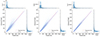 |
Fig. 6. Pixel-to-pixel comparison for three different models. Left panel: Results for the 642 case. Middle panel: Results for 1282 case. Right panel: Results for the 2562 case. The variance shrinks with increasing input resolution. The corresponding Pearson statistics are 0.9879, 0.9936 and 0.9961. The axes of the main plots show pixel values. The margin plots indicate the 1D distributions along the corresponding axes. |
For all the images, we measured all the metrics from Section 4.1 and built Figure 7 based on the calculations we made. In addition to previous conclusions, we highlight that the x256 model (green line) outperforms all the models, but in general, both x256 and x128 seem to be numerically stable and ready to use on any adequately qualitative image from the chosen cycle, as all the statistics are quite good: PCC strongly tends to 1, RE oscillates around 0 with a deviation of nearly a tenth of a %, SSIM tends to 1, but the PPE10 is only acceptable for the x256 model and strongly deteriorates for the other resolutions. An intriguing observation arises when considering the temporal alignment of our images precisely at their respective creation times, denoted by the strictly ascending order of points on the X-axis. Notably, a subtle decline in statistical measures emerges after approximately 60 images, corresponding to the temporal threshold of 2017 and onward. This epoch coincides with a discernible reduction in solar intensity within the solar cycle. This shows that the last decade presented a trend, which is borne out not only by our hypothesis that the application of these models to other solar cycles may yield a notable reduction in accuracy, but is primarily due to the selection of a solar cycle that was characterized by significantly reduced activity. Conversely, we anticipate satisfactory results by employing the same models within the context of the training cycle even with this simplified approach.
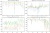 |
Fig. 7. PCC and RE of summed pixel values, PPE10, and SSIM for spatial super-resolution models on the dataset consisting of 98 test images from every year from the chosen cycle. The dotted blue line corresponds to the x64 model, the dashed orange line shows the 128x model, and the solid green line shows the metrics values for the 256x model. All the statistics depend on the resolution and become better as it increases, which correlates with previous inferences. |
The execution time for every trained model was around 0.004 seconds for an Nvidia Tesla T4.
4.3. Temporal reconstruction
4.3.1. Baseline model
To evaluate the temporal reconstruction model, it is important to consider previous works that focused on generating solar images Park et al. (2019). However, these works primarily concentrated on mapping the magnetogram into UV or EUV bands, which does not allow a fair comparison to our model. To address this limitation, we propose a baseline model that computes the differential rotation of the Sun with the rotational profile developed by Howard et al. (1990) as implemented in the SunPy package.
4.3.2. Data analysis
Figure 8 shows a randomly sampled ground image in the 171 Å channel and its corresponding predicted image by the UNet model. The model learns the structures and patterns of active and quiet regions in the disk region and the growth and recession of flares on the limb. The right image in Figure 8 shows the difference between the real and predicted images, where dark red and blue colors represent the regions with the largest differences. The loss shown in the bright regions is higher, justifying the need to assign a higher weight to these regions.
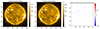 |
Fig. 8. Randomly selected pair of ground (left) and predicted (middle) images in the 171 Å channel. The images were clipped to the [0, 99] percentile range and their square roots were taken to enhance the contrast to illustrate the pattern better. The difference between the actual pixel values of the two images is displayed on the right, and the minimum and maximum values are indicated in the color bar. |
In addition, we present scatter plots in Figure 9, illustrating the predicted values against real values for each pixel across 100 samples in the evaluation dataset. The distribution of the predicted images generally agrees with the ground images. The scattering of low and high predicted values against high and low ground values is due to the mismatched position of the flaring region at the pixel level.
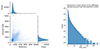 |
Fig. 9. Comparison of the differences in pixel value distributions between the ground truth and the predictions. Panel a: Pixel-to-pixel comparison between the predicted values and ground values of the solar images in a curated dataset. This dataset consisted of 100 randomly selected samples from the evaluation dataset. The figure shows a large difference between the predicted values and the real values, which arises because the model underestimates the intensity of the flaring region, and a mismatch in the flaring region also results in a large difference as the nonflaring region is quiet. Panel b: Distribution of the pixel values for the difference tensor between the ground truth and the prediction for the x256 model. The number of higher pixel values decreases rapidly and is nearly 102 per 20 for values between 0 and 40. |
The same power spectrum and transfer function fractional errors (TFFE) analysis was carried out on the model outputs and the dataset used for the temporal reconstruction in Figure A.1. While the power spectra of the outputs and data exhibited different numerical characteristics, their TFFEs exhibited a similar trend, with the errors oscillating around zero at the large scale and starting to exaggerate around k = 150. This shows that the model outputs capture the details at the large scale and start to deviate at a smaller scale.
4.3.3. Result table
Table A.1 in Appendix A shows the RE, PPE10, and SSIM of the entire evaluation dataset, with the model interpolating a single frame. The baseline model obtains a high score in the evaluation metrics, indicating that the patterns on the solar disk evolve linearly within the short timescale. The extremely small RE and high PPE10 indicate that the total magnitude on the solar disk remains unchanged. However, compared to the first three metrics, the baseline model does not perform as well in the SSIM metric. This was expected because the interpolation between the first and third frames contains all possible distributions of patterns in the second frame, resulting in a blurrier structure.
The high PCC indicates that our model is able to capture the general movement of the patterns on the solar disk. The overall high values in PCC also suggest that it might not be an ideal performance metric in this type of comparison. Although its RE is significantly higher than that of the baseline model, the order of magnitude of RE remains rather small. The overall high PPE10 and SSIM values indicate that the model captures the development of the pattern in fine detail. In general, our model is able to predict images that lie within the real distribution while maintaining the structure of patterns on the solar disk.
The performance of the baseline model also significantly deteriorates when we attempted to interpolate longer sequences. This suggests that the patterns on the solar disk no longer adhere to a linear progression on a larger timescale. In contrast, our model demonstrates only a slight drop in performance with increasing input length, indicating its ability to capture the nonlinearity in pattern development on the solar disk, particularly over extended periods.
The model performed worse in the 94 Å, 131 Å, and 335 Å passbands. This may be attributed to the fact that sunlight emissions in these passbands primarily occur in the active or flaring regions of the corona, which have lower irradiance levels. Consequently, these passbands exhibit a lower pixel value on the disk compared to others, as depicted in Figure 10. This might indicate a low signal-to-noise ratio, and the model may therefore find it challenging to recognize patterns on the solar disk in these passbands, resulting in convergence failure.
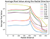 |
Fig. 10. Average pixel values calculated in the radial direction for the passbands with low pixel values on the disk, namely 94 Å, 131 Å, and 335 Å, and for other passbands with high pixel values on the disk. The peaks observed are attributed to the limb region of the Sun, with the disk radius measured at 204 pixels. |
It is also worth mentioning that there is a sudden drop in the PPE10 score for our model at 193 Å and 211 Å for certain input lengths. This indicates that numerical instability remains an issue for the model convergence on specific subsets of data, resulting in outputs with incorrect distributions at the pixel level.
4.4. Discussion
Our findings demonstrate notable improvements in solar image quality through our approach. Compared with previous investigations, such as those presented in Rahman et al. (2020), the authors employed a very deep residual neural network with over 400 layers to upsample from 1282 to 5122. While the training time for their model was not specified in the paper, our model, which consists of only 35 layers, achieved comparable results with a higher resolution step and used half the number of training data. The SSIM averaged across the main part of our dataset (excluding the lowest part of the solar cycle, where all trained models performed poorly) is ≈0.98, 0.93, 0.91 for 642, 1282, and 2562, respectively, compared to 0.98 for the 1282 to 5122 model from Rahman et al. (2020). Similar results were observed for the PCC, where our 2562 and 1282 models outperform by this metric, while the 642 model underperforms slightly. In Yang et al. (2023), the authors explored various CNN-based architectures, including UNet-based models. While mapping 1282 to 5122, they achieved a best model SSIM of 0.9709, which is slightly outperformed by our UNet-based architecture in the case of the 2562 model and is comparable for the 642 and 1282 models. The study presented in Song et al. (2024) demonstrated another UNet-based implementation using multiple attention layers. For this case, the SSIM metric in our work shows a significant improvement across all three models.
5. Conclusions
We demonstrated that a UNet-based architecture can be employed to enhance the spatial and temporal resolution of solar images through pixel-wise comparisons of images and different evaluation metrics that achieved notable results. Higher-quality solar images are significant for advancing our understanding of solar dynamics and facilitates accurate space weather prediction. Our work represents a step toward a fine-grained resolution of solar features, enabling the qualitative characterization and tracking of transient phenomena such as solar flares, coronal mass ejections, and magnetic field evolution.
However, substantial potential remains for further advancements. Future research could explore contemporary super-resolution techniques, such as incorporating attention mechanisms (Vaswani et al. 2023) and leveraging advanced machine-learning methods such as diffusion models (Ho et al. 2020). While diffusion-based architectures have been investigated by various authors (Song et al. 2023, 2024), the reported metrics, such as SSIM, were less favorable than our simplified UNet-based approach. These methods also required significantly longer training times because they are complex. Nevertheless, their potential should not be overlooked. The primary limitation of our models lies in their reduced precision when capturing fine details. We hypothesize that this issue could be addressed by incorporating attention mechanisms that focus on specific regions of solar activity. Additionally, diffusion-based techniques might enhance the model ability to generalize. However, implementing these features is challenging because these methods often require significant training time and may result in suboptimal inference speeds. Careful consideration of these trade-offs is necessary to determine whether these advanced techniques can be integrated in the future.
Data availability
We will provide the code for implementing the models and evaluation metrics used in this paper for spatial super-resolution at https://github.com/alexgugnin/solar_superres and for temporal reconstruction at https://colab.research.google.com/drive/1wfghvEj7WMBG1ITXz643lIPom2mmumxt?usp=sharing
Acknowledgments
The authors acknowledge the Center for Computational Astrophysics of the Flatiron Institute provided resources that have contributed to the research results reported within this paper. Work of O. Gugnin was supported by the National Research Foundation of Ukraine under project No. 2023.03/0149.
References
- Cai, Z., Zhong, Z., & Zhang, B. 2023, New Astron., 101, 102018 [NASA ADS] [CrossRef] [Google Scholar]
- Dash, A., Ye, J., Wang, G., & Jin, H. 2022, Ann. Data Sci., 11, 1545 [Google Scholar]
- Domingo, V., Fleck, B., & Poland, A. I. 1995, Space Sci. Rev., 72, 81 [Google Scholar]
- Galvez, R., Fouhey, D. F., Jin, M., et al. 2019, ApJS, 242, 7 [Google Scholar]
- Goodfellow, I. J., Pouget-Abadie, J., Mirza, M., et al. 2014, ArXiv e-prints [arXiv:1406.2661] [Google Scholar]
- Hanslmeier, A., & Messerotti, M. 1999, Proceedings of the Summerschool and Workshop held at the Solar Observatory, Kanzelhöhe, Kärnten, Austria, 1 [Google Scholar]
- Ho, J., Jain, A., & Abbeel, P. 2020, ArXiv e-prints [arXiv:2006.11239] [Google Scholar]
- Howard, R. F., Harvey, J. W., & Forgach, S. 1990, Sol. Phys., 130, 295 [NASA ADS] [CrossRef] [Google Scholar]
- Jindal, V., Liang, A., Singh, A., Ho, S., & Jamieson, D. 2023, ArXiv e-prints [arXiv:2303.13056] [Google Scholar]
- Kaiser, M. L., Kucera, T. A., Davila, J. M., et al. 2008, Space Sci. Rev., 136, 5 [Google Scholar]
- Lemen, J. R., Title, A. M., Akin, D. J., et al. 2011, Sol. Phys., 275, 17 [Google Scholar]
- Mumford, S. J., Freij, N., Stansby, D., et al. 2023, https://doi.org/10.5281/zenodo.8384174 [Google Scholar]
- Park, E., Moon, Y.-J., Lee, J.-Y., et al. 2019, ApJ, 884, L23 [NASA ADS] [CrossRef] [Google Scholar]
- Pesnell, W. D., Thompson, B. J., & Chamberlin, P. C. 2012a, Sol. Phys., 1, 12 [Google Scholar]
- Pesnell, W. D., Thompson, B. J., & Chamberlin, P. C. 2012b, The Solar Dynamics Observatory (New York: Springer) [Google Scholar]
- Rahman, S., Moon, Y. J., Park, E., et al. 2020, ApJ, 897, L32 [NASA ADS] [CrossRef] [Google Scholar]
- Rimmele, T., Warner, M., Keil, S., et al. 2020, Sol. Phys., 295, 172 [NASA ADS] [CrossRef] [Google Scholar]
- Ronneberger, O., Fischer, P., & Brox, T. 2015, Medical Image Computing and Computer-Assisted Intervention – MICCAI 2015 (Cham: Springer International Publishing), 234 [Google Scholar]
- Salvatelli, V., Bose, S., Neuberg, B., et al. 2019, ArXiv e-prints [arXiv:1911.04006] [Google Scholar]
- Song, W., Ma, W., Ma, Y., et al. 2023, ApJS, 263, 25 [Google Scholar]
- Song, W., Ma, Y., Sun, H., Zhao, X., & Lin, G. 2024, A&A, 686, A272 [NASA ADS] [CrossRef] [EDP Sciences] [Google Scholar]
- Therese, A. K. 2015, Stereo – Solar Conjunction Science, https://stereo-ssc.nascom.nasa.gov/solar_conjunction_science.shtml [Google Scholar]
- Vaswani, A., Shazeer, N., Parmar, N., et al. 2023, ArXiv e-prints [arXiv:1706.03762] [Google Scholar]
- Wang, Z., Bovik, A. C., Sheikh, H. R., & Simoncelli, E. P. 2004, IEEE Trans. Image Process., 13, 600 [Google Scholar]
- Yang, Q., Chen, Z., Tang, R., Deng, X., & Wang, J. 2023, ApJS, 265, 36 [NASA ADS] [CrossRef] [Google Scholar]
Appendix A: Metrics for temporal super-resolution
PCC, RE, PPE10, and SSIM values for Each passband with the input length as 3,5,7,9, respectively
 |
Fig. A.1. Power spectra and transfer function fractional errors (TFFE) for models’ targets and predictions across nine channels. Solid, dotted, and dashed lines in the left figures represent average power spectra for the evaluation set. Shades around lines are sigma ranges. In the right figures, the solid line represents the average TFFE for the prediction/target. This time, shades represent functional errors through partial derivatives. |
All Tables
PCC, RE, PPE10, and SSIM values for Each passband with the input length as 3,5,7,9, respectively
All Figures
|
Fig. 1. UNet-based architecture used for the temporal reconstruction of solar images, where n represents the input length of the solar image sequence. Each box corresponds to a multichannel feature map. The gray boxes are copied maps. The number of channels is shown at the top of the box. The resolution in pixels is indicated at the side of the box. The arrows represent operations. A similar architecture is also used in spatial super-resolution, but with only three pairs of double convolutional blocks, and a dropout rate of 0.25 is introduced at each convolutional layer. |
| In the text | |
|
Fig. 2. Comparative performance plot across various models. From top to bottom, the rows delineate three distinct models characterized by progressively higher resolution inputs. From left to right, the columns depict the input image, prediction, and ground truth, respectively. |
| In the text | |
|
Fig. 3. Power spectra and transfer function fractional errors (TFFE) for all three models. The solid, dotted, and dashed lines in the left column represent average power spectra for the whole test set (target, input, and prediction, respectively). The shading around the lines shows the sigma ranges. In the right column, the solid line represents the average TFFE for the prediction and the target, and the dashed line represents the same for the baseline and the target. This time, the shading represents the functional errors through partial derivatives. |
| In the text | |
|
Fig. 4. Comparison between the input low-resolution image (2562 resolution), shown in the left panel, and the predicted image in the middle (10242 resolution). The third panel shows the pixel-wise difference between the ground truth and the resulting image. A larger difference corresponds to higher values in the residual plot (the hotter color of the color map). The model performs better in more intensive regions. |
| In the text | |
|
Fig. 5. Pair of columns depicting various data representations. The top left panel shows the disparity between the ground truth and the prediction within the mean plus three standard deviation intervals for the pixel values of the model with the resolution of 64 → 1024. The lower section displays a difference map with all pixel values. The right column exhibits analogous relations, but for the model employing a higher-resolution input. |
| In the text | |
|
Fig. 6. Pixel-to-pixel comparison for three different models. Left panel: Results for the 642 case. Middle panel: Results for 1282 case. Right panel: Results for the 2562 case. The variance shrinks with increasing input resolution. The corresponding Pearson statistics are 0.9879, 0.9936 and 0.9961. The axes of the main plots show pixel values. The margin plots indicate the 1D distributions along the corresponding axes. |
| In the text | |
|
Fig. 7. PCC and RE of summed pixel values, PPE10, and SSIM for spatial super-resolution models on the dataset consisting of 98 test images from every year from the chosen cycle. The dotted blue line corresponds to the x64 model, the dashed orange line shows the 128x model, and the solid green line shows the metrics values for the 256x model. All the statistics depend on the resolution and become better as it increases, which correlates with previous inferences. |
| In the text | |
|
Fig. 8. Randomly selected pair of ground (left) and predicted (middle) images in the 171 Å channel. The images were clipped to the [0, 99] percentile range and their square roots were taken to enhance the contrast to illustrate the pattern better. The difference between the actual pixel values of the two images is displayed on the right, and the minimum and maximum values are indicated in the color bar. |
| In the text | |
|
Fig. 9. Comparison of the differences in pixel value distributions between the ground truth and the predictions. Panel a: Pixel-to-pixel comparison between the predicted values and ground values of the solar images in a curated dataset. This dataset consisted of 100 randomly selected samples from the evaluation dataset. The figure shows a large difference between the predicted values and the real values, which arises because the model underestimates the intensity of the flaring region, and a mismatch in the flaring region also results in a large difference as the nonflaring region is quiet. Panel b: Distribution of the pixel values for the difference tensor between the ground truth and the prediction for the x256 model. The number of higher pixel values decreases rapidly and is nearly 102 per 20 for values between 0 and 40. |
| In the text | |
|
Fig. 10. Average pixel values calculated in the radial direction for the passbands with low pixel values on the disk, namely 94 Å, 131 Å, and 335 Å, and for other passbands with high pixel values on the disk. The peaks observed are attributed to the limb region of the Sun, with the disk radius measured at 204 pixels. |
| In the text | |
|
Fig. A.1. Power spectra and transfer function fractional errors (TFFE) for models’ targets and predictions across nine channels. Solid, dotted, and dashed lines in the left figures represent average power spectra for the evaluation set. Shades around lines are sigma ranges. In the right figures, the solid line represents the average TFFE for the prediction/target. This time, shades represent functional errors through partial derivatives. |
| In the text | |
Current usage metrics show cumulative count of Article Views (full-text article views including HTML views, PDF and ePub downloads, according to the available data) and Abstracts Views on Vision4Press platform.
Data correspond to usage on the plateform after 2015. The current usage metrics is available 48-96 hours after online publication and is updated daily on week days.
Initial download of the metrics may take a while.