| Issue |
A&A
Volume 698, June 2025
|
|
|---|---|---|
| Article Number | A263 | |
| Number of page(s) | 15 | |
| Section | Numerical methods and codes | |
| DOI | https://doi.org/10.1051/0004-6361/202453627 | |
| Published online | 20 June 2025 | |
Tracking the photospheric horizontal velocity field with shallow U-net models
1
National Key Laboratory of Deep Space Exploration, School of Earth and Space Sciences, University of Science and Technology of China,
Hefei
230026,
China
2
CAS Center for Excellence in Comparative Planetology/CAS Key Laboratory of Geospace Environment/Mengcheng National Geophysical Observatory, University of Science and Technology of China,
Hefei
230026,
China
3
Planetary Environmental and Astrobiological Research Laboratory (PEARL), School of Atmospheric Sciences, Sun Yat-sen University,
Zhuhai,
China
4
School of Data Science, Qingdao University of Science and Technology,
Qingdao
266061,
China
5
Yunnan Observatories, Chinese Academy of Sciences,
Kunming
650216,
China
★ Corresponding author: This email address is being protected from spambots. You need JavaScript enabled to view it.
Received:
30
December
2024
Accepted:
29
April
2025
Abstract
Context. Understanding the horizontal velocity field of the highly magnetized plasma within the solar atmosphere is essential to understanding the complicated dynamics and energy evolution of solar phenomena at various scales, from small-scale swirls to coronal mass ejections. Most traditional methods estimate the photospheric horizontal velocity field by tracking bright features. These reconstructed velocity fields may differ from the ground truth because the photosphere is not a single layer but has a depth of ~500 km. The observed bright features are combined emissions from different heights in the photosphere.
Aims. In this work, we aim to develop a series of models for tracking the photospheric horizontal velocity field with high accuracy from high-resolution observations using a modified shallow U-Net architecture and to evaluate the performance of different models.
Methods. We used photospheric intensity, vertical magnetic field strength, and horizontal velocity fields from a realistic 3D radiative numerical simulation of a quiet-Sun region generated using the Bifrost code to train and validate the shallow U-Net models. We built three shallow U-Net models: an intensity model using photospheric intensity as the input, a magnetic model using vertical magnetic field strength as the input, and a hybrid model combining both.
Results. All three models yield good performances, among which the hybrid model shows the best performance with a correlation coefficient of 0.85 with the ground-truth velocity field. Comparisons with the Fourier local correlation tracking (FLCT) and the DeepVel methods demonstrate the superiority of the shallow U-Net models. Based on the research of this work, we have released a software named SUVEL for public use to extract photospheric horizontal velocity fields from high-resolution observations. SUVEL is only designed to be used on photospheric observations in the quiet-Sun regions with high temporal (best at 10 s, preferably less than 50 s) and high spatial resolutions.
Key words: Sun: atmosphere / Sun: general / Sun: photosphere
© The Authors 2025
 Open Access article, published by EDP Sciences, under the terms of the Creative Commons Attribution License (https://creativecommons.org/licenses/by/4.0), which permits unrestricted use, distribution, and reproduction in any medium, provided the original work is properly cited.
This article is published in open access under the Subscribe to Open model. This email address is being protected from spambots. You need JavaScript enabled to view it. to support open access publication.
1 Introduction
Tracking the velocity field of highly magnetized solar plasma is a key objective in understanding the complicated dynamics at various layers of the solar atmosphere from the photosphere to the corona. Understanding plasma motions provides vital information about the Sun’s dynamic behavior, magnetic activities, and the resulting space weather phenomena that can impact the Earth. The movement of plasma in the solar atmosphere, especially the photosphere, where the plasma β > 1, is closely related to a range of phenomena from small scales to large scales, including the generation and propagation of vortices and Alfvén pulses (e.g., Wang et al. 1995; Velli & Liewer 1999; Bonet et al. 2008; Attie et al. 2009; Shelyag et al. 2011, 2013; Requerey et al. 2018; Liu et al. 2019c,d; Tziotziou et al. 2023), the emergence and evolution of sunspots (e.g., Evershed 1910; Brown et al. 2003; Yan & Qu 2007; Su et al. 2008; Bi et al. 2016; Gou et al. 2024), the formation and propagation of spicules and jets (see e.g., Sterling 2000; Pariat et al. 2009; Matsumoto & Shibata 2010; Raouafi et al. 2016; Liu et al. 2016; Huang et al. 2019; Tian et al. 2021; Dey et al. 2022), and the initiation and dynamics of solar flares and coronal mass ejections (CMEs) (e.g., Nindos & Zhang 2002; Schrijver 2009; Chen 2011; Shen et al. 2012; Wang et al. 2018; Georgoulis et al. 2019; Zhou et al. 2022). Understanding the plasma velocity field helps to elucidate the complex interactions between the Sun’s magnetic fields and plasma, providing insights into the processes that govern solar activities.
The solar plasma’s line-of-sight (LOS) velocity component can be obtained using spectroscopic observations. Space-borne observatories such as Hinode (Kosugi et al. 2008), the Interface Region Imaging Spectrograph (IRIS, De Pontieu et al. 2014), and the Chinese Hα Solar Explorer (CHASE, Li et al. 2022), and ground-based telescopes including the Swedish Solar Telescope (SST, Scharmer et al. 2003), the New Vacuum Solar Telescope (NVST, Liu et al. 2014), and the Daniel K. Inouye Solar Telescope (DKIST, Rimmele et al. 2020) provide high-resolution spectroscopic data that allow for precise measurements of Doppler shifts at various heights of the solar atmosphere, offering estimates of the velocity along the line of sight. These measurements are critical for investigating the solar atmosphere’s velocity structure and impact on solar features with different spatial and temporal scales. Numerous significant findings have been made based on the Doppler velocities obtained from spectral observations of the solar atmosphere. This topic is among the most important in solar and stellar physics research. We will not list all the literature due to the vast number of papers, but readers are encouraged to look into some relevant research. Nevertheless, the LOS velocity alone is insufficient for a complete characterization of the solar plasma flows, as it only provides a projection of the velocity along the observer’s viewing angle and neglects the horizontal components of the velocity field.
Various techniques have been developed to map the horizontal velocity field at the solar photosphere. For studies involving a limited number of features or events, the horizontal velocity field could be measured using manual methods such as constructing the time-distance plots along the propagating direction of the target motions. While effective for specific applications, these manual methods are time-consuming and lack automation. Thus, automated processes have been introduced. For example, one of the most widely used techniques is the Fourier local correlation tracking method (FLCT, Welsch et al. 2004; Fisher & Welsch 2008). Local correlation tracking (LCT) methods estimate the 2D horizontal velocity field by calculating the correlation between the intensity (brightness) features in two successive images taken within a short interval. Despite its successful applications in tracking solar horizontal velocity fields, studies have shown that FLCT usually underestimates the actual speed and should be used with caution (e.g., Verma et al. 2013; Louis et al. 2015). Another disadvantage of FLCT when applied to photospheric observations is that the estimated velocity field may be biased because the observed photospheric intensity is generally an integration of the emission over the LOS, i.e., the observed features in the images may not be located at the same layer.
One way to bypass FLCT’s above shortcomings is to use the photospheric magnetic field to estimate its horizontal velocity field (e.g., Schuck 2006, 2008). The most used methods are the differential affine velocity estimator (DAVE, Schuck 2006) for the LOS magnetic field observations and DAVE4VM (Schuck 2008) for the vector magnetic field observations. DAVE and DAVE4VM have been extensively used to reconstruct the horizontal velocity fields, especially in active regions. These reconstructed horizontal velocity fields can be used to estimate the variations of the magnetic energy, helicity, and magnetic twist (e.g., Kusano et al. 2002; Berger & Field 1984; Liu et al. 2013a; Tziotziou et al. 2015; Wang et al. 2017; Liu et al. 2018; Korsós et al. 2022), as well as the input of realistic data-driven numerical simulations (e.g., Liu et al. 2019a).
One shortcoming of these traditional methods is the relatively slow calculation speed, though parallelization techniques have been used. In recent years, deep learning techniques have shown great promise in automating the tracking of the solar horizontal velocity fields. Masaki et al. (2023) proposed to estimate the horizontal velocity field using one intensity image at only a specific moment for the input of a neural network. Despite the relatively low correlation coefficient between the evaluated and the ground-truth velocities, the physics of how the velocity field could be derived from one intensity map instead of at least two consecutive ones remains questionable. Asensio Ramos et al. (2017) and Tremblay & Attie (2020) employed two different neural network architectures and built models named DeepVel and DeepVelU with the numerical simulation data as their inputs to estimate the horizontal velocity field. Although the performances were found to be good, the temporal (30 s) and spatial (48 km pixel−1) resolutions were relatively low. This was later improved by Ishikawa et al. (2022), whose temporal and spatial resolutions are 35 s and 42 km, respectively. Instead of using numerical simulation data to train the neural networks, Shang et al. (2023) developed a model based on PWCNet to estimate the horizontal velocity field specifically from the Hα and TiO observations by NVST. Considering that the highest available (and future) spatial resolution provided by DKIST (Rimmele et al. 2020), the European Solar Telescope (EST, 4-m aperture, under construction, Collados et al. 2013), and the Chinese Giant Solar Telescope (CGST, 8-m aperture, actively promoted, Liu et al. 2013b) (will) have pixel scales of 10–20 km, a neural network model able to reconstruct the photospheric horizontal velocity field from these extremely high-resolution observations is urgently needed. Moreover, most of the above models only use the intensity data as their inputs. The contribution of the photospheric magnetic field strength in estimating the horizontal velocity field is not considered.
In this paper, we introduce a new method for tracking the photospheric horizontal velocity field from observations with high temporal and spatial resolutions using shallow U-Net models, a convolutional neural network known for its efficacy in image segmentation tasks (Ronneberger et al. 2015). The shallow U-Net architecture, with its relatively small number of layers compared to the original U-Net architecture, offers a promising trade-off between computational efficiency and model performance. The built models will take simultaneous data of the photospheric intensity and LOS magnetic field strength as input to achieve better performance. The rest of this paper is organized as follows: Data and methods will be described in Sect. 2, with the results presented in Sect. 3, followed by the comparison and generalization test in Sect. 4, and conclusions and discussions in Sect. 5.
2 Data and methods
The data utilized for training and testing in this work is from a realistic numerical simulation of a quiet-Sun region by the Bifrost code (Gudiksen et al. 2011). Bifrost was built by considering the radiative transfer effect in the energy balance equation, with the capability of solving the Magnetohydrodynamics (MHD) equation in three-dimensional space. It has been applied to realistically simulate active regions, quiet-Sun regions, and more in a variety of studies (see, e.g. Carlsson et al. 2016). The simulation data employed to train and validate the neural networks are bounded in a 6 Mm × 6 Mm quiet-Sun region with a 2.93 km pixel size located at the photosphere (τ500 = 1, where τ500 is the optical depth at 500 nm), resulting in 2048× 2048 pix2 in the field of view (FOV). There are 440 frames in the dataset with a temporal cadence of 10 s.
Considering the pixel size of the photospheric observations with the highest resolution is ~12 km at the TiO passband by DKIST (e.g., Rimmele et al. 2020) with currently the world’s largest aperture (4 m) of solar observations, the original numerical simulation data is then downgraded by a factor of 4, resulting in data cubes of 440 × 512 × 512 pix3 for each physical parameter contained in the simulation with a pixel size of 11.71 km. The physical parameters used in this work are photospheric intensity (I), vertical magnetic field strength (Bz), plasma speed along the x-axis (vx), and plasma speed along the y-axis (vy). The photospheric intensity I is the intensity of the continuum bin in the multi-group opacity method (Nordlund 1982), and there is no meaningful physical unit for the photospheric intensity obtained from the simulation. I is then normalized to [0, 1] based on its maximum (0.3) and minimum values (0.15). The vertical magnetic field strength Bz has a maximum value of 1891 G (auss) and a minimum value of −1807 G. Considering that about 98% of Bz has an absolute value less than 200 G, Bz is capped between [−200 G, 200 G] and then normalized to [0, 1]. The horizontal velocities (vx and vy) have maximum and minimum values of 11.5 km/s and −10.4 km/s. To maximize the generalization of the models to be built when applied to new data, the units of vx and vy are converted to pixel per frame (PPF) and then normalized to [0, 1] between −10 PPF and 10 PPF.
The distributions of all the above physical parameters are checked individually in each frame before the normalization, and frames with invalid or infinite values are omitted to maintain the sanity of the whole dataset. To allow the models used to capture more small-scale details in the input images, each frame (with a size of 512 × 512 pix2) is divided into 4×4 equal-sized patches, resulting in patches with a size of 128 × 128 pix2. Examples of these patches are depicted in Figure 1, showing the overall framework of the built models, which will be detailed below. As one can see from Figure 1, there are in total three models built: Model 1 (the intensity model) taking three successive frames of I as the input, Model 2 (the magnetic model) taking three consecutive frames of Bz as the input, and Model 3 (the hybrid model) taking both I and Bz together with the outputs of Models 1 and 2 as the input. The outputs of these three models are the reconstructed horizontal velocity fields vx and vy, but are given different symbols (subscripts i for the intensity model, m for the magnetic model, and h for the hybrid model) to distinguish between their outputs. To obtain the velocity field at time t, three frames of the intensity (vertical magnetic field strength) at t − δt, t, and t + δt are needed for Model 1 (Model 2), where δt = 10 s is the cadence of the simulation. These six frames (three frames of the intensity and three frames of the vertical magnetic field strength), together with the outputs (four frames) of Model 1 and Model 2, are combined to serve as the input of Model 3 (see Fig. 1). These models are built with shallow U-Net architectures.
The original U-Net convolutional neural network was proposed by Ronneberger et al. (2015) and applied to the segmentation task for biomedical images. It was named “U-Net” because its architecture resembles the letter “U.” There have been several different variations of U-Net that revealed good performances in various tasks, including “Attention U-Net” with attention gates added to the architecture (Oktay et al. 2018), “TransUNet” to enable explicit modeling of the long-range dependency in images (Chen et al. 2021), and many more. Besides its success in other fields, U-Net has also been used for solar and space physics research. For example, Liu et al. (2024) developed an automated jet detection algorithm to find off-limb coronal jets based on the U-Net architecture. Zheng et al. (2024) employed a U-Net model to identify and track filaments from the Hα observations by the Chinese H α Solar Explorer (CHASE, Li et al. 2022). An automated and bias-free sunspot detection method was recently proposed by Chen et al. (2025), which is also based on the U-Net architecture. After a series of trial-and-error tests, we found that the original U-Net and TransUNet would lead to over-fitting (good performance in the training set but lousy performance in the validation set) with the specific inputs in this work. Thus, adapted from the original U-Net, we have designed a shallow U-Net architecture depicted in Figure 2. We demonstrate that the shallow U-Net architecture, with its relatively small number of layers compared to the original U-Net, offers a promising trade-off between computational efficiency and model performance.
The light yellow block on the top left in Figure 2 represents the input, which has a size of 128 × 128 × n, where n = 3 for Models 1 and 2 and n = 10 for Model 3. In the first step, the input image is fed into two convolutional layers, each having 64 filters with a kernel size of 3 × 3. In each layer, the Rectified Linear Unit (ReLU) activation function is used after each convolutional operation, where ReLU(x) = max(0, x). The resulting image after the first step is then down-sampled to 64 × 64 by a max pooling operation (purple arrows in Fig. 2), where only the maximum value in every 2 × 2 region in the image is kept, and all other pixels are discarded. This operation is added to increase the ability of the architecture to fit nonlinear relations and to minimize the chance of over-fitting. The image is then taken into the next step, which contains two convolutional layers with 128 filters.
The above process is repeated with the number of filters doubling each step until the image size is down-sampled to 16 × 16 with 512 filters. Then, a reverse series of operations of the above process (yellow arrows in Fig. 2) is performed and skip connected to the left part of the shallow U-Net to up-sample the image until it has a size of 128 × 128. These skip connections remind the shallow U-NET of the previously learned fine details. Two extra convolutional layers, both with two filters, are used to generate the final output images with a size of 128 × 128 × 2, where the first and second channels of the last dimension are vx and vy, respectively (see the blue block in Fig. 2). The architecture’s left (right) part is often called the encoder (decoder).
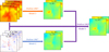 |
Fig. 1 Flow chart of the three shallow U-Net models. Photospheric intensity and vertical magnetic field (Bz) data are from the numerical simulation detailed in the main text. Three models are illustrated in this flow chart. Model 1 (intensity model) takes three consecutive frames of the photospheric intensity as input. Model 2 (magnetic model) takes three successive frames of the photospheric vertical magnetic field strength as input. Model 3 (hybrid model) combines the inputs and outputs of Model 1 and Model 2 as its input. The outputs of the three models are images with two channels; the first channel is the velocity field along the x direction (vx) and the second channel is the velocity field along the y direction (vy). Here, δt represents the cadence of the data (10 s). Subscripts i, m, and h denote outputs of the intensity, magnetic, and hybrid models, respectively. |
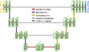 |
Fig. 2 Architecture of the shallow U-Net. This figures is a modification of Figure 2 in Liu et al. (2024). See Sect. 2 for a detailed description of the shallow U-NET architecture. |
3 Results
After removing invalid patches with infinite or invalid values, the final dataset built contains 6843 sets of instances. As illustrated above, each instance includes eight images, i.e., three consecutive images of the photospheric intensity (I), three successive images of the photospheric vertical magnetic field strength (Bz), and two images of the horizontal velocity field (vx and vy). The dataset is then randomly shuffled and divided into two parts: the training set (~80%, 5458 instances) and the validation set (~20%, 1385 instances). The training set is used to train the shallow U-Net models, resulting in the intensity model (Model 1), the magnetic model (Model 2), and the hybrid model (Model 3). The validation set is employed to evaluate the performance of the above three models. Panels a1–a4 in Figure 3 are examples of one instance in the dataset with vx in panel a1, vy in panel a2, intensity in panel a3, and Bz in panel a4. The vector velocity field is also visualized as black arrows in panel a3. It is noted that all three models are trained independently, while Model 3 takes the input and output of Models 1&2 as its input. These models are trained with up to 1000 epochs, with the training process stopped when the loss of the validation set does not improve within 50 epochs.
In this section, we will describe the training and validation results of the intensity model before presenting the training and validation of the magnetic and hybrid models.
3.1 The intensity model
The target of training a neural network is minimizing the loss function between the output and the ground truth labels. In the case of tracking the photospheric horizontal velocity fields, the labels are vx and vy from the numerical simulation, and the task of the built shallow U-Net model is to reconstruct a horizontal velocity field as similar to the ground truth as possible. This means choosing a suitable loss function and the learning rate (the step size at which the optimization algorithm updates the model’s parameters during training) is critical to finding and building the most accurate model.
Table 1 lists the evaluation metrics of the intensity model on the validation set with different learning rates. The loss functions are MS E (mean square error), MAE (mean absolute error), MAS E (a combination of MS E and MAE), and a customized loss function LCOS. The definitions of these loss functions are:
![Mathematical equation: $\[M S E=\frac{1}{N} \sum\left[\left(v_{x i}-v_x\right)^2+\left(v_{y i}-v_y\right)^2\right],\]$](/articles/aa/full_html/2025/06/aa53627-24/aa53627-24-eq1.png) (1)
(1)
![Mathematical equation: $\[M A E=\frac{1}{N} \sum\left[\left|v_{x i}-v_x\right|+\left|v_{y i}-v_y\right|\right],\]$](/articles/aa/full_html/2025/06/aa53627-24/aa53627-24-eq2.png) (2)
(2)
![Mathematical equation: $\[M A S E=M A E+\alpha \cdot M S E,\]$](/articles/aa/full_html/2025/06/aa53627-24/aa53627-24-eq3.png) (3)
(3)
![Mathematical equation: $\[L C O S=M A E+\beta \cdot(1-C O S).\]$](/articles/aa/full_html/2025/06/aa53627-24/aa53627-24-eq4.png) (4)
(4)
Here, vx (vxi) and vy (vyi) are the ground truth (reconstructed values by the intensity model) of the horizontal velocity field in the x direction and y direction. N is the number of pixels in all instances in the validation set. COS is the average cosine of the angle (θ) between the reconstructed velocity field and the ground truth, which is defined as
![Mathematical equation: $\[\operatorname{COS}=\frac{1}{N} \sum \frac{v_{x i} \cdot v_x+v_{y i} \cdot v_y}{\sqrt{v_{x i}^2+v_{y i}^2} \cdot \sqrt{v_x^2+v_y^2}+\epsilon},\]$](/articles/aa/full_html/2025/06/aa53627-24/aa53627-24-eq5.png) (5)
(5)
where ϵ is a small number used to avoid division by zero. α and β in the above equations are used to scale the different losses into the same order of magnitude. Running some test pieces of training revealed that the MAE is, on average, 10 times larger than the MS E and 10 times larger than 1 − COS. So, both α and β have been set to 10 in this work.
The first row in Table 1 lists the evaluation metrics used. They are the RMS E (square root of MS E, Eq. (1)), MAE (Eq. (2)), and COS (Eq. (5)). Note that the RMS E and MAE in the evaluation metrics are rescaled to have their units as pixel per frame (PPF) to allow an intuitive sense of the actual errors in the velocity fields. CC is the correlation coefficient between the estimated and ground-truth velocity fields, ranging from −1 to 1, which considers the pixel-to-pixel relation in the images. S S IM is the structural similarity between the reconstructed and ground-truth velocity fields. It is based on comparing three measurements associated with the pixel values, contrast, and structure. A value close to 1 indicates the two compared images have high similarity. Details on the definition of S S IM can be found in Equations (2)–(13) in Wang et al. (2004).
Considering that the maximum values of vx and vy are less than 10 PPF, 10 pixels at each boundary of the images will be omitted in calculating the evaluation metrics for all the models in the rest of this paper. In practice, the velocity field of these omitted pixels could be easily recovered by having overlaps of at least 20 pixels in each direction when cutting a bigger FOV into patches with a size of 128 × 128 pix2. For each of the four loss functions, we train a series of shallow U-Net models with different learning rates 10−4, 1−3, 10−2, 10−1) as the initial value of the Adaptive Gradient (Adagrad) optimizer (e.g., Ward et al. 2018). These models for each loss function are then evaluated based on the above evaluation metrics, and only the model with the best performance is kept. The second column in Table 1 shows the learning rate that results in the best performance with different loss functions. It is seen that although different loss functions lead to models with similar performances, the model with MAS E as the loss function (Eq. (3)) and a learning rate of 0.01 leads to a better result. The RMS E and MAE of the intensity model are as low as ~1.04 PPF and ~0.79 PPF, respectively. This means that the reconstructed velocity field (vxi and vyi) is on average 1 PPF away from the ground-truth velocity field (vx and vy). COS is very close to 1, indicating that the reconstructed velocity field points in almost the same direction as the ground-truth velocity field on most pixels. CC and S S IM are ~0.78 and 0.79, respectively, suggesting the high correlation and structural similarity between the reconstructed and ground-truth velocity fields.
Panels b1, b2, and the black arrows in panel b3 in Figure 3 are one example of the reconstructed velocity field. Compared with panels a1–a3, one can find that the overall distributions of the reconstructed and ground-truth velocity fields are very similar, with the reconstruction lacking some detailed structures. This is consistent with the fact that most deviations happen at locations with many small-scale structures, as seen as the green areas in the cos(θ) distribution (Fig. 3b3). Figure 3b4 shows the difference (residual) between the absolute value of the reconstructed (vi) and the ground truth (v) velocity fields. In most cases, the absolute difference is less than 1 PPF with maximum values less than 3 PPF, which is consistent with what we have found in the evaluation metrics MAE and RMS E.
Figure 4a1 is the pixel-to-pixel relation between the reconstructed vxi by the intensity model and the ground truth vx. Colors in Figure 4a1 depict the number density distribution of all points in the scatter plot, with warmer colors denoting higher number densities. Most points are located at the diagonal, indicating good alignment between the reconstructed and the ground-truth velocity fields. A good linear relation can be seen with a of 0.80. The slope (1.08) is very close to 1 with an intercept of 0.22, meaning that the intensity model generally overestimates vx slightly. These observations are the same for the velocity field along the y direction (Fig. 4a2). Panel a3 in Figure 4 is the distribution of the angle (θ) between the reconstructed by the intensity model and the ground-truth velocity fields. In most (~82%) cases, the angle is less than 50°, showing the good alignment between the directions of the reconstructed and the ground-truth velocity fields. In only 7% cases, the angle is above 90°.
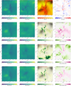 |
Fig. 3 Example velocity fields by the shallow U-Net models. Panels in the first column are the ground-truth vx (a1) and estimated vx by the intensity model (b1), magnetic model (c1) and hybrid model (d1), respectively. Panels in the second column are similar to panels in the first column, but for the velocity field along the y direction (vy). The background in panel (a3) shows the photospheric intensity with the black arrows depicting the vector velocity field. Panel (a4) represents the photospheric vertical magnetic field strength. Backgrounds in panels (b3)–(d3) are the cosine of the angle (θ) between the estimated and ground-truth velocity field by the three shallow U-Net models, with the black arrows depicting the estimated vector velocity fields by the models. Panels (b4)–(d4) are the distributions of the velocity differences between the ground-truth and estimated velocity fields by the three shallow U-Net models. |
Evaluation metrics for the intensity model.
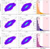 |
Fig. 4 Correlation between the Shallow U-Net velocity fields and the ground truth. Panels (a1), (b1) and (c1) are the pixel-to-pixel correlations between the ground-truth vx and the model estimated vx by the three shallow U-Net models. Colors in these panels depict the number densities of points at each coordinate, with warmer colors for higher number densities. Black dashed lines are the corresponding linear fit results, with their functions displayed on the top left corner of each panel. Panels (a2), (b2), and (c2) are similar to panels (a1), (b1), and (c1) but for vy. Panels (a3), (b3), and (c3) are the distribution of the angles between the ground-truth velocity fields and the estimated velocity fields by the three shallow U-Net models. |
3.2 The magnetic and hybrid models
Unlike the intensity model (Model 1), the magnetic model (Model 2) takes three consecutive frames of the vertical magnetic field strength as its input (Fig. 1). However, similar to the intensity model, the final magnetic model is also selected from a series of models with different loss functions and learning rates. The second row in Table 2 lists the loss function and learning rate used to build the best magnetic model and its evaluation metrics. The magnetic model performs slightly better than the intensity model (first row in Table 2). The RMS E drops to less than 1 (0.96 PPF), with the MAE dropping from 0.79 PPF to 0.74 PPF. CC and S S IM rise from 0.78 and 0.79 by the intensity model to 0.81 and 0.80 by the magnetic model, respectively.
Panels c1–c2 in Figure 3 exhibit the reconstruction by the magnetic model (with three successive frames centered at the vertical magnetic field shown in Fig. 3a4) of the velocity field in Figures 3a1–a3. Compared to the velocity field given by the intensity model in Figures 3b1–b2, the velocity field given by the magnetic model reveals more detailed structures that are consistent with the ground-truth velocity field in panels a1–a2. Although the direction of the reconstructed velocity field shows more deviation from the ground-truth velocity field for this particular instance, evidenced by the distribution of cos(θ) in Figure 3b3, the overall alignment between the reconstructed and ground-truth velocity fields are better in the magnetic field model (COS = 0.998 in the second row in Table 2). Comparison between Figures 3b4 and 3c4 reveals that in regions where the intensity model overestimates the velocity, the magnetic model mainly underestimates it. This indicates that a model considering both the intensity and magnetic field strength would probably perform better. This is indeed the case for the hybrid model, which is detailed below.
Figure 4b1 is the pixel-to-pixel relation between the reconstructed vxm by the intensity model and the ground truth vx. Again, most points are located at the diagonal, showing good alignment between the reconstructed and ground-truth velocity fields. A better linear relation can be seen with an improved CC of 0.82, compared to that of the intensity model in Figure 4a1. The slope (0.99) is almost 1 with an intercept of −0.08, showing no systematic overestimation or underestimation of vx by the magnetic model. The performance of the magnetic model on predicting vy (Fig. 4b2) is not as good as its performance on predicting vx, but still better than the performance of the intensity model. Panel b3 in Figure 4 is the distribution of the angle (θ) between the reconstructed by the magnetic model and ground-truth velocity fields. It reveals very similar results with the intensity model that in most (~82%) cases, the angle is less than 50°, and in only 7% cases, the angle is above 90°.
The hybrid model (Model 3) takes advantage of the information provided by both the photospheric intensity and vertical magnetic field strength. It takes three frames of the intensity, three frames of the vertical magnetic field strength, the output (vxi and vyi) of the intensity model, and the output (vxi and vyi) of the magnetic model as its input to reconstruct the horizontal velocity field (vx and vy) at the simulated photosphere. Fed with this additional information, the hybrid model is expected to perform better than the intensity and magnetic models. This is proven by the evaluation metrics in the third row of Table 2. The best model is again found to be built with MAS E as the loss function and a learning rate of 0.01. The RMS E and MAE are further reduced to 0.84 PPF and 0.64 PPF, respectively. The hybrid model improves CC and S S I M to 0.85 and 0.83, respectively. These improvements in the evaluation metrics are also evidenced by the example in Figures 3d1–d4. The velocity fields (vxh and vyh) in Figures 3d1–d2 have more details than those reconstructed by the intensity (Figs. 3b1–b2 or the magnetic model (Figs. 3c1–c2) and are more similar to the ground truth in Figures 3a1–a2. There are much fewer pixels with values less than 0 in the cos(θ) distribution (Fig. 3d3), suggesting that the hybrid model could produce velocity fields that are more aligned with the ground truth. The residual velocity norm (vh - v) is also further reduced (Fig. 3d4).
The correlations between the reconstructed velocity field by the hybrid model and the ground-truth velocity field are shown in Figures 4c1 and c2. The correlation coefficients are further improved to 0.86 and 0.84 for vx and vy, respectively. The slope between vx (vy) and vxh (vyh) is 1.00 (1.04) with an intercept of – 0.07 (−0.02). This means the hybrid model does not overestimate or underestimate the horizontal velocity fields. In 87% cases, the angle between the reconstructed and the ground-truth velocity fields is below 50°, and in only 5% cases, the angle is above 90°.
Evaluation metrics for all presented models in this work.
4 Comparison and generalization tests
In this section, we will describe a series of benchmark tests between the three models mentioned above and two other models built on traditional and neural network methods. Further tests of the generalization ability of the three shallow U-Net models on the noisy data and data from a different numerical simulation are also presented in this section.
4.1 Comparison with FLCT
As described in the introduction, the Fourier Local correlation tracking (FLCT, Welsch et al. 2004; Fisher & Welsch 2008) method has been widely used to estimate the horizontal velocity field at various layers from the photosphere to the corona in the solar atmosphere since its inception. Many research papers have proven its success, and in this subsection, we will apply FLCT to the particular numerical simulation data employed in this paper, evaluate its performance using the evaluation metrics introduced in the above subsections, and compare it with the shallow U-Net models constructed in this paper. The version of FLCT used is v1.06, with the threshold and low-pass spatial filtering left undefined. Following suggestions in literature (e.g. Louis et al. 2015; Liu et al. 2019c) and to be consistent with that the maximum velocity norm in the data is less than 10 PPF, the pixel width of the Gaussian filter (sigma) is also set to 10. A new feature in v1.06 is to add the bias correction to the calculation. Preliminary tests by Liu et al. (2019b) suggest that turning on the bias correction can increase the calculated horizontal velocity field strength by ~80%, but still underestimate the actual velocity field by a factor of ~3. In the rest of this subsection, we will discuss the velocity fields estimated by FLCT with the photospheric intensity (labeled as FLCT-I) and vertical magnetic field (labeled as FLCT-M) as its input, respectively.
Panels in the first row in Figure 5 show an example instance of the estimated velocity field (vxfi and vyfi) by FLCT-I whose ground truth is shown in the first row of Figure 3. A direct comparison between Figures 5a1–a2 and Figures 3a1–a2 reveals that FLCT-I only recovers very little of the original velocity field. Zero to negative values of cos(θ), which represent large angles (90° to 180°) between the directions of the estimated and ground-truth velocity fields, are almost randomly distributed throughout the whole FOV. The residuals of the velocity norm are relatively high, with absolute values up to 5 PPF, while the absolute velocity residuals of the shallow U-Net models are below 3 PPF. Figures 5b1–b4 are similar to Figures 5a1–a4, but are results of FLCT-M. It is hard to see which of FLCT-I and FLCT-M performs better, but we can find the answer from their statistics in Figure 6.
Figure 6 is similar to Figure 4 but for velocity fields estimated by FLCT-I (panels a1–a3) and FLCT-M (panels b1–b3). The correlation between the velocity field (vxfi and vyfi) given by FLCT-I and the ground-truth velocity field (vx and vy) is barely above 0.20. The slopes of the linear fit (black dashed lines in Figs. 6a1 and a2) are both 0.16, suggesting that FLCT-I underestimates the horizontal velocity field by a factor of about 6. The number density distributions of all points in the scatter plot (colors in Figs. 6a1 and a2) also show the poor alignment between the estimated and ground-truth velocity fields. In ~46% cases, the angle between the FLCT-I estimated velocity field and the ground-truth velocity field is less than 50°, and in 32% cases, the angle is above 90° (Fig. 6a3). The performance of FLCT-M is better with CCs above 0.5 (Figures 6b1 and b2). The slopes of the linear fit (black dashed lines in Figs. 6b1 and b2) are around 0.5, indicating that FLCT-M only underestimates the photospheric horizontal velocity field by a factor of 2. The better performance of FLCT-M over FLCT-I is also seen in the number density distributions in Figures 6b1–b2, as well as in Figure 6b3, where in 62% cases the angle between the FLCT-M reconstructed velocity field and the ground-truth velocity field is less than 50°, and in 19% cases, the angle is above 90°.
The middle two rows in Table 2 list the evaluation metrics of FLCT-I and FLCT-M. The RMS E and MAE for FLCT-I (FLCT-M) are ~1.71 PPF (~1.67 PPF) and ~1.34 PPF (~1.08 PPF), respectively. The alignment between the reconstructed velocity field and the ground-truth velocity field is worse than that of the shallow U-Net models with COS as 0.993 and 0.995, respectively, for FLCT-I and FLCT-M. CC and S S IM of FLCT-I are only ~0.23 and ~0.66. The performance of FLCT-M is better with a CC of ~0.52 and an S S IM of ~0.67. The poor performance of FLCT-I is expected because the photospheric intensity is an integration of the combined emission at different heights in the photosphere. Features in the photospheric intensity images would indicate the plasma motion not only at the τ500 = 1 layer but also at other layers. Horizontal velocity fields derived by FLCT from comparing the intensities at different frames are likely not the same as the horizontal velocity field at the τ500 = 1 layer. These findings that FLCT performs better when taking the magnetic field strength as the input than when taking the intensity as the input is consistent with what was found in Li et al. (2023).
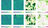 |
Fig. 5 Example velocity fields by FLCT. Panels are similar to their corresponding panels in Figure 3. FLCT-I (FLCT-M) represents the resulting velocity fields by the FLCT with the photospheric intensity (vertical magnetic field strength) as the input. |
4.2 Comparison with DeepVel
The neural network architecture DeepVel proposed by Asensio Ramos et al. (2017), as mentioned in the introduction, also takes numerical simulation data as inputs to train the network. Although the model (hereafter referred to as the original DeepVel) trained on the simulation data with a cadence of 60 s and a pixel size of 96 km may not be fit for other simulation data and observations, Asensio Ramos et al. (2017) suggested retraining DeepVel on data with corresponding temporal and spatial resolutions may improve its performance. Therefore, following the instructions available at their repository1, a version of DeepVel (hereafter referred to as the retrained DeepVel) with new weight parameters was retrained using our training set described in Sect. 2. It is noted that the two versions of DeepVel both use MS E as the loss function with the same learning rate of 10−4, as shown in Table 2 following the suggestions by Asensio Ramos et al. (2017). Similar to Sect. 4.1, we will employ both the original DeepVel and the retrained DeepVel to our validation set, to evaluate their performances using the five evaluation metrics in Table 2, and make comparisons with the shallow U-Net models proposed in this work.
The linear fit between the velocity field (vxod and vyod) reconstructed by the original DeepVel and the ground-truth velocity (vx and vy) show slopes of 2.28 and 2.17, with intercepts of 0.23 and 0.33, respectively. The slopes suggest that the original DeepVel overestimates the horizontal velocity by a factor of ~2. CCs between the estimated and the ground-truth velocity fields are found to be 0.62 and 0.56, for vx and vy respectively, indicating that the original DeepVel reconstructs the velocity field with decent linear relations. On the other hand, the velocity field (vxrd and vyrd) estimated by the retrained DeepVel show better linear fits with the ground-truth velocity field, with slopes of 1.07 and 1.22 (closer to 1), suggesting that the scale of the velocity field estimated by the retrained DeepVel is comparable to the ground truth. The better performance of the retrained DeepVel also proves the future potential of DeepVel by being retrained with new training data.
The evaluation metrics of the original DeepVel and retrained DeepVel are listed in the bottom two rows in Table 2. Consistent with the above results, the RMS E and MAE for the retrained DeepVel are ~1.50 PPF and ~1.20 PPF, less than ~3.17 PPF and ~2.57 PPF for the original DeepVel, respectively. COS s (0.980 and 0.994) are both near 1, but still less than those of the shallow U-Net models proposed in this work. CC and S S IM of the original DeepVel (retrained DeepVel) are not optimal, with values of ~0.59 (~0.53) and ~0.53 (~0.67), respectively. The poor performance of the two versions of DeepVel compared to the shallow U-Net models proposed in this paper might have been caused by the limitation of the neural network structure of DeepVel.
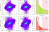 |
Fig. 6 Correlation between the FLCT velocity fields and the ground truth. Panels are similar to panels in Figure 4 but for the results of FLCT-I (top) and FLCT-M (bottom). |
4.3 Generalization test
Noting that DeepVel exhibits less optimal performance when handling simulation and observational data with different temporal resolutions (Asensio Ramos et al. 2017), a natural question is if the shallow U-Net models proposed in this work are also affected by different temporal resolutions. To examine the generalization ability of the shallow U-Net models, in this subsection, we will test them with data from another realistic 3D radiative numerical simulation framework – the CO5BOLD code (Freytag et al. 2012).
Based on a relaxed, purely hydrodynamical model with an initial vertical and homogeneous magnetic field of 50 G, data from the CO5BOLD code simulating the surface layers of the Sun are bounded in a 9.6 × 9.6 × 2.8 Mm3 box, with a pixel size of 10 km. The height of the box (2.8 Mm) is large enough to include the surface layers of the convection zone, the photosphere, and up to the middle chromosphere (Cuissa & Steiner 2024). In this subsection, only the simulation data at the photospheric layer (~1400 km from the bottom of the box) is utilized for testing the shallow U-Net models. In total, 26 frames are obtained from the simulation with a cadence of 240 s.
Notably, the data contains the vertical magnetic field (Bz) at different heights, but only includes the sum of photospheric intensity over all heights. Therefore, only the magnetic model (Model 2) is applied to track the photospheric horizontal velocity in the CO5BOLD simulation. Since vx and vy in the training data are capped between [−10 PPF, 10 PPF] ([−11.7 km/s, 11.7 km/s]) and normalized to [0, 1], we could then re-scale the output (vxm and vym) of Model 2 to the real velocity (vxmr and vymr) in units of km/s by using the following relations:
![Mathematical equation: $\[\begin{aligned}& v_{x m r}=v_{x m} \cdot 23.4-11.7, \\& v_{y m r}=v_{y m} \cdot 23.4-11.7.\end{aligned}\]$](/articles/aa/full_html/2025/06/aa53627-24/aa53627-24-eq6.png) (6)
(6)
By comparing the reconstructed velocity field (vxmr and vymr) given by Model 2 (Figs. 7b1–b2) and the ground-truth velocity field (vx and vy, Figs. 7a1–a2), it can be found that different structures and small details of the velocity field are mostly successfully detected by Model 2. Moreover, the scales of vxmr and vymr are comparable to vx and vy (both concentrating between −10 km/s and 10 km/s), proving the reliability of Eq. (6). Considering that Eq. (6) is irrelevant to spatial and temporal resolutions, it can generally be utilized for different observational and simulation data.
However, the slopes of linear fits between vxmr (vymr) and vx (vy) are 3.53 (4.39), suggesting that Model 2 overestimated the velocity field by a factor of ~4 (see Figs. 7c1–c2). The correlation coefficients drop to 0.36 and 0.35 for vx and vy, respectively. It is natural to speculate that the poor performance of Model 2 on CO5BOLD simulation data might be caused by the longer cadence (240 s) than our Bifrost simulation training data (10 s), given their similar pixel sizes (~11 km vs. ~10 km).
To study the influence of different cadences on the performance of the shallow U-Net models, we can manually increase the cadence of the instances in the validation set from the Bifrost numerical simulation. For instance, for the velocity of the image at time t, its next image is selected at t + n · δt and its previous image is chosen at t − n · δt, where δt = 10 s and n represents the number of frames skipped in the original validation set. In this way, we manually increase the cadence of the inputs and calculate the evaluation metrics obtained from the hybrid model (Model 3, see Fig. 8). When the cadence increases, RMS E and MAE both increase, while CC and S S IM both decline. It’s noted that, when the cadence increases to 240 s (equal to the cadence of CO5BOLD simulation data used above), RMS E and MAE reach 2.4 PPF and 2.0 PPF, respectively. Meanwhile, CC drops quickly to about 0.16, and S S IM slowly decreases to 0.56. The rapidly increasing RMS E and MAE explain the overestimated velocity field by the shallow U-Net models on CO5BOLD simulation data. And the slowly decreasing value (0.56) of S S IM is consistent with the results that different structures and small details are mostly detected. It is also noted that CC stays above 0.5 and MAE is still less than 1.5 PPF even when the cadence is downgraded to 50 s.
In conclusion, these results suggest that the shallow U-Net models in this work focus on the velocity reconstruction from data with high cadences (~10 s to 50 s) which are common for the current and forthcoming solar telescopes with large apertures (e.g., DKIST, EST, and CGST as mentioned in the introduction). Their performance is expected to be less optimal when the cadence increases.
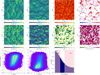 |
Fig. 7 Example velocity fields by Model 2 and their correlation with the ground truth derived from CO5BOLD simulation. Panels (a) and (b) are similar to their corresponding panels in Figures 3 and 5. Panels (c) are similar to panels in Figures 4 and 6 but for the results of Model 2 applied to the CO5BOLD simulation data. |
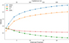 |
Fig. 8 Evaluation parameters of Model 3 (the hybrid model) with different cadences. The bottom x-axis represents the number of the interval frames used to increase the cadence (see the main text), and the top x-axis is the corresponding cadence. The definition of the evaluation metrics (RMS E, MAE, CC, and S S IM) can be found in the main text. RMS E and MAE have units of pixel per frame (PPF). CC and S S IM are unitless. |
4.4 Performance on noisy data
It is worth noting that the data utilized for training and testing in this work are both from a noise-free Bifrost numerical simulation without spatial degradation. Different from the ideal simulation data, high-resolution observational data collected from 4 to 8 m class ground-based telescopes (e.g., DKIST, EST, and CGST) are subject to atmospheric effects, diffraction, and thus noise. To examine the performance of the shallow U-Net models on noisy observational data, in this subsection, we test them with a generated test set by adding 10% noise into the original test set.
The photospheric intensity (I) of the simulation in this work has the maximum value of 0.3, as mentioned in Sect. 2, and approximately 99.8% of the vertical magnetic field strength (Bz) has an absolute value below 200 G. However, it is noticed that ~84% of the values of Bz range between [–50 G, 50 G]. Therefore, to generate the noisy test data, Gaussian noises with intensity values in the range of [−0.03, 0.03] and Bz values in [−5 G, 5 G] are randomly added into the original test data. Then, the shallow U-Net models are employed to reconstruct the velocity field from the noisy test data.
Figure 9 shows the velocity fields at the same time instance but reconstructed by the three different shallow U-Net models (panels a1–a3 for Model 1, panels b1–b3 for Model 2, and panels c1–c3 for Model 3). The ground truth of these velocity fields is shown in the first row of Figure 3. Comparisons with the bottom three rows of Figure 3 suggest that the introduced 10% noise does affect the performance of the Shallow U-Net models in both the direction (Figs. 9a3–c3) and the absolute value (Figs. 9a4–c4) of the estimated velocity field, although the difference are subtle. Figure 10 further shows the influence of noise on the performance of the shallow U-Net models, i.e., decreases in the correlation coefficients (CCs) and deteriorations in the linear regressions compared to Figure 3. Nevertheless, the shallow U-Net models still perform well on the generated noisy test data. For instance, for the hybrid model (Model 3), CCs of vx and vy remain high at 0.78 and 0.76, with slopes close to 1 (0.98 and 1.05) and intercepts close to 0 (−0.03 and −0.02, see Fig. 10). The distributions of the angle θ between the velocity field reconstructed by the three models and the ground truth are highly consistent with the distribution from the noise-free data (see Figs. 9 and 3). In most cases (~66% to ~78%), the angle is less than 50 degrees, while in only ~10% to ~15% of the cases it exceeds 90 degrees. Again, the performance of the hybrid model is, as expected, better than that of the intensity and magnetic models.
Therefore, the shallow U-Net models, especially the hybrid model proposed in this work, demonstrate robust performance on simulation data with a 10% noise, suggesting their applicability to the solar observational data. In the future, it is worth looking into how different noise levels would affect the performance of the shallow U-Net models.
5 Conclusions and discussion
In this paper, we introduce three neural network models to obtain the horizontal velocity field in the solar photosphere. These three models are built upon a realistic 3D MHD numerical simulation of the solar photosphere with a shallow U-Net architecture. The first model takes three consecutive images of the photospheric intensity as its input and achieves a correlation coefficient of 0.78 with the ground-truth velocity field. The second model takes three successive images of the vertical magnetic field strength as its input and achieves a correlation coefficient of 0.80 with the ground-truth velocity field. The third model takes both the inputs and outputs of the first two models, takes advantage of additional information provided by different measurements, and achieves a correlation coefficient of 0.85 with the ground-truth velocity field. These models are named the intensity model, the magnetic model, and the hybrid model, respectively.
Despite the good correlation between the ground-truth velocity field and the estimated velocity fields by the three models, analysis shows that the built shallow U-Net models do not overestimate or underestimate the velocity field. Most importantly, but often overlooked in the literature, we have also investigated the distribution of the angles between the estimated and the ground-truth velocity fields. It is found that in most cases (82–87%), the angle is below 50°, indicating that the reconstructed velocity field of the shallow U-Net models is in good alignment in terms of their vector directions with the ground-truth velocity field. This is vital in many tasks sensitive to the directions of the velocity vectors, such as automated detection of photospheric small-scale swirls (e.g. Liu et al. 2019c).
As a benchmark test, the horizontal velocity field is also estimated by FLCT with the intensity (FLCT-I) and the magnetic field strength (FLCT-M) as the input. FLCT-I reveals a correlation coefficient of 0.23, indicating a poor performance in processing high-resolution photospheric intensity observations. FLCT-M performs better with a correlation coefficient of 0.52, but is still significantly lower than the shallow U-Net models in this work. A deep learning approach for estimating the velocity field named DeepVel is also utilized for comparisons. The horizontal velocity field is reconstructed by the DeepVel built by Asensio Ramos et al. (2017) (original DeepVel) and the version retrained on our training data (retrained DeepVel). The Original DeepVel overestimates the velocity field by a factor of ~2, while the Retrained DeepVel shows a limited improvement of the performance. The lower correlation coefficients (0.59 and 0.53) of these two models with the ground-truth velocity fields suggest the superiority of the shallow U0Net models over the DeepVel models.
Another numerical simulation data from CO5BOLD code with different temporal (240 s) resolutions is applied to the shallow U-Net models, aiming to check their generalization abilities on data with different temporal resolutions. Comparisons between the model-generated and the ground-truth velocity field suggest that different cadences do affect the performance of the shallow U-Net models. But downgrading the cadence of the Bifrost numerical simulation data to 50 s still keeps the CC above 0.5. Moreover, we also test the Shallow U-Net models with a generated test dataset with a 10% noise level to examine their performance on noisy data. By comparing the results estimated from the 10%-noise test data with results from the noise-free data, it is found by the studied evaluation metrics that a 10% noise has little influence on the performance of the Shallow U-Net models when reconstructing the velocity field. The distribution of the angles θ between the estimated velocity field and the ground truth also further proves the robustness of the shallow U-Net models, with a 10% noise introduced. One of our future works is to study the influence of different noise levels on the performance of the shallow U-Net models.
These three pre-trained shallow U-Net models introduced in this paper have been integrated into a user-friendly software named SUVEL available at our Github repository2. This tool takes three successive images of the photospheric intensity or (and) the LOS magnetic field strength as its input. When only the photospheric intensity (magnetic field strength) is provided, the intensity (magnetic) model will be used. When both the intensity and magnetic field strength are supplied as the input, the hybrid model will be used to estimate the horizontal velocity field. It is noted that all the inputs shall be capped with certain upper and lower limits and then normalized to [0, 1] before being fed to SUVEL. The upper and lower limits for the magnetic field observations are suggested to be ±200 G. The upper and lower limits for the photospheric intensity observations shall depend on the data. We demonstrate that SUVEL is superior to FLCT in terms of not only the similarity with the ground-truth velocity field but also the calculation speed. On a test machine with a 24-core Intel i9 12900 K CPU and a modern GPU, it takes SUVEL less than 2 seconds to estimate the horizontal velocity field for the validation set with 1385 instances. The processing time needed for FLCT on the same dataset is ~8 minutes.
It is worth noting that though the hybrid model exhibits good performance, its output still has some deviations from the ground truth (see, e.g., the last row in Fig. 3), especially at locations with many very small-scale structures. Figure 11 shows the variation of the evaluation metrics when the velocity fields are downsampled to different scales with different downsampling factors. The blue, orange, green, and red curves in Figure 11 are for the RMS E, MAE, CC, and S S IM, respectively. Both RMS E and MAE drop rapidly when the downsampling factor rises and the pixel scale increases. The RMS E reaches 0.61 PPF, and the MAE drops to 0.49 PPF when the pixel scale is increased to ~160 km. Meanwhile, CC and S S IM increase when the pixel scale increases. CC and S S IM could be improved to 0.89 and 0.90, respectively, when the pixel scale is ~160 km. These results suggest that SUVEL performs better in reconstructing the velocity field of larger-scale structures. Here, larger scale corresponds to structures with a typical size of ~100 km, which in most cases is still considered small scale. Future work will focus on further improving the model performance and introducing physics constraints in the models.
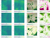 |
Fig. 9 Example velocity fields by the Shallow U-Net models but for the generated noisy test data. Panels are similar to their corresponding panels in Figure 3, but for the results of the Shallow U-Net models from the noisy test data. |
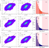 |
Fig. 10 Correlation between the Shallow U-Net velocity fields from the generated noisy test data and the ground truth. Panels are similar to panels in Figure 4 but for the results of the Shallow U-Net models from the noisy test data. |
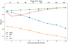 |
Fig. 11 Evaluation parameters of Model 3 (the hybrid model) with different pixel sizes. The bottom x-axis represents the downsampling factor of the velocity field in the validation set, and the top x-axis is the corresponding pixel scale at different downsampling factors. The definition of the evaluation metrics (RMS E, MAE, CC, and S S IM) can be found in the main text. RMS E and MAE have units of pixel per frame (PPF). CC and S S IM are unitless. |
Acknowledgements
We thank Prof. Mats Carlsson at the University of Oslo for providing the numerical simulation data used in this work. J.L. and C.Z. acknowledge the support from the National Natural Science Foundation (NSFC 42188101) and the Strategic Priority Research Program of the Chinese Academy of Science (Grant No. XDB0560000). Jiajia Liu also acknowledges support from the National Natural Science Foundation (NSFC 12373056). Yimin Wang acknowledges the support from the National Natural Science Foundation of China (NSFC 12303103).
References
- Asensio Ramos, A., Requerey, I. S., & Vitas, N. 2017, A&A, 604, A11 [NASA ADS] [CrossRef] [EDP Sciences] [Google Scholar]
- Attie, R., Innes, D. E., & Potts, H. E. 2009, A&A, 493, L13 [NASA ADS] [CrossRef] [EDP Sciences] [Google Scholar]
- Berger, M. A., & Field, G. B. 1984, J. Fluid Mech., 147, 133 [NASA ADS] [CrossRef] [Google Scholar]
- Bi, Y., Jiang, Y., Yang, J., et al. 2016, Nat. Commun., 7, 13798 [Google Scholar]
- Bonet, J. A., Márquez, I., Sánchez Almeida, J., Cabello, I., & Domingo, V. 2008, Astrophys. J. Lett., 687, L131 [Google Scholar]
- Brown, D. S., Nightingale, R. W., Alexander, D., et al. 2003, Solar Phys., 216, 79 [Google Scholar]
- Carlsson, M., Hansteen, V. H., Gudiksen, B. V., Leenaarts, J., & De Pontieu, B. 2016, A&A, 585, A4 [NASA ADS] [CrossRef] [EDP Sciences] [Google Scholar]
- Chen, P. 2011, Living Rev. Solar Phys., 8, 1 [NASA ADS] [CrossRef] [Google Scholar]
- Chen, J., Lu, Y., Yu, Q., et al. 2021, arXiv e-prints [arXiv:2102.04306] [Google Scholar]
- Chen, J., Gyenge, N. G., Jiang, Y., et al. 2025, ApJ, 980, 261 [Google Scholar]
- Collados, M., Bettonvil, F., Cavaller, L., et al. 2013, Mem. Soc. Astron. Italiana, 84, 379 [NASA ADS] [Google Scholar]
- Cuissa, J. C., & Steiner, O. 2024, A&A, 682, A181 [NASA ADS] [CrossRef] [EDP Sciences] [Google Scholar]
- De Pontieu, B., Title, A., Lemen, J., et al. 2014, Solar Phys., 289, 2733 [Google Scholar]
- Dey, S., Chatterjee, P., OVSN, M., et al. 2022, Nat. Phys., 18, 595 [CrossRef] [Google Scholar]
- Evershed, J. 1910, MNRAS, 70, 217 [NASA ADS] [Google Scholar]
- Fisher, G. H., & Welsch, B. T. 2008, ASP Conf. Ser., 383, 373 [NASA ADS] [Google Scholar]
- Freytag, B., Steffen, M., Ludwig, H.-G., et al. 2012, J. Computat. Phys., 231, 919 [NASA ADS] [CrossRef] [Google Scholar]
- Georgoulis, M. K., Nindos, A., & Zhang, H. 2019, Philos. Trans. Roy. Soc. A, 377, 20180094 [Google Scholar]
- Gou, T., Liu, R., Su, Y., et al. 2024, Sol. Phys., 299, 99 [Google Scholar]
- Gudiksen, B. V., Carlsson, M., Hansteen, V. H., et al. 2011, A&A, 531, A154 [NASA ADS] [CrossRef] [EDP Sciences] [Google Scholar]
- Huang, Z., Li, B., & Xia, L. 2019, Solar-Terrestrial Phys., 5, 58 [Google Scholar]
- Ishikawa, R. T., Nakata, M., Katsukawa, Y., Masada, Y., & Riethmüller, T. L. 2022, A&A, 658, A142 [NASA ADS] [CrossRef] [EDP Sciences] [Google Scholar]
- Korsós, M., Erdélyi, R., Huang, X., & Morgan, H. 2022, ApJ, 933, 66 [CrossRef] [Google Scholar]
- Kosugi, T., Matsuzaki, K., Sakao, T., et al. 2008, The Hinode Mission (Springer), 5 [Google Scholar]
- Kusano, K., Maeshiro, T., Yokoyama, T., & Sakurai, T. 2002, ApJ, 577, 501 [NASA ADS] [CrossRef] [Google Scholar]
- Li, C., Fang, C., Li, Z., et al. 2022, Sci. China Phys. Mech. Astron., 65, 289602 [NASA ADS] [CrossRef] [Google Scholar]
- Li, Q., Xu, Y., Verma, M., et al. 2023, Sol. Phys., 298, 62 [Google Scholar]
- Liu, Y., Zhao, J., & Schuck, P. 2013a, Solar Phys., 287, 279 [Google Scholar]
- Liu, Z., Deng, Y., & Ji, H. 2013b, Proc. Int. Astron. Union, 8, 349 [Google Scholar]
- Liu, Z., Xu, J., Gu, B.-Z., et al. 2014, Res. Astron. Astrophys., 14, 705 [Google Scholar]
- Liu, J., Wang, Y., Erdélyi, R., et al. 2016, ApJ, 833, 150 [NASA ADS] [CrossRef] [Google Scholar]
- Liu, L., Cheng, X., Wang, Y., et al. 2018, ApJ, 867, L5 [Google Scholar]
- Liu, C., Chen, T., & Zhao, X. 2019a, A&A, 626, A91 [NASA ADS] [CrossRef] [EDP Sciences] [Google Scholar]
- Liu, J., Carlsson, M., Nelson, C. J., & Erdélyi, R. 2019b, A&A, 632, A97 [NASA ADS] [CrossRef] [EDP Sciences] [Google Scholar]
- Liu, J., Nelson, C. J., & Erdélyi, R. 2019c, ApJ, 872, 22 [Google Scholar]
- Liu, J., Nelson, C. J., Snow, B., Wang, Y., & Erdélyi, R. 2019d, Nat. Commun., 10, 3504 [Google Scholar]
- Liu, J., Ji, C., Wang, Y., et al. 2024, ApJ, 972, 187 [Google Scholar]
- Louis, R. E., Ravindra, B., Georgoulis, M. K., & Küker, M. 2015, Sol. Phys., 290, 1135 [NASA ADS] [CrossRef] [Google Scholar]
- Masaki, H., Hotta, H., Katsukawa, Y., & Ishikawa, R. T. 2023, PASJ, 75, 1168 [Google Scholar]
- Matsumoto, T., & Shibata, K. 2010, ApJ, 710, 1857 [NASA ADS] [CrossRef] [Google Scholar]
- Nindos, A., & Zhang, H. 2002, ApJ, 573, L133 [NASA ADS] [CrossRef] [Google Scholar]
- Nordlund, A. 1982, A&A, 107, 1 [Google Scholar]
- Oktay, O., Schlemper, J., Le Folgoc, L., et al. 2018, arXiv e-prints [arXiv:1804.03999] [Google Scholar]
- Pariat, E., Antiochos, S., & DeVore, C. 2009, ApJ, 691, 61 [Google Scholar]
- Raouafi, N., Patsourakos, S., Pariat, E., et al. 2016, Space Sci. Rev., 201, 1 [NASA ADS] [CrossRef] [Google Scholar]
- Requerey, I. S., Cobo, B. R., Gošić, M., & Rubio, L. R. B. 2018, A&A, 610, A84 [NASA ADS] [CrossRef] [EDP Sciences] [Google Scholar]
- Rimmele, T. R., Warner, M., Keil, S. L., et al. 2020, Sol. Phys., 295, 172 [Google Scholar]
- Ronneberger, O., Fischer, P., & Brox, T. 2015, arXiv e-prints [arXiv:1505.04597] [Google Scholar]
- Scharmer, G. B., Bjelksjo, K., Korhonen, T. K., Lindberg, B., & Petterson, B. 2003, in Proc. SPIE, 4853, Innovative Telescopes and Instrumentation for Solar Astrophysics, eds. S. L. Keil, & S. V. Avakyan, 341 [Google Scholar]
- Schrijver, C. J. 2009, Adv. Space Res., 43, 739 [NASA ADS] [CrossRef] [Google Scholar]
- Schuck, P. W. 2006, ApJ, 646, 1358 [Google Scholar]
- Schuck, P. W. 2008, ApJ, 683, 1134 [NASA ADS] [CrossRef] [Google Scholar]
- Shang, Z.-H., Mu, S.-Y., Ji, K.-F., & Qiang, Z.-P. 2023, Res. Astron. Astrophys., 23, 065009 [Google Scholar]
- Shelyag, S., Fedun, V., Keenan, F. P., Erdélyi, R., & Mathioudakis, M. 2011, Ann. Geophys., 29, 883 [Google Scholar]
- Shelyag, S., Cally, P. S., Reid, A., & Mathioudakis, M. 2013, Astrophys. J. Lett., 776, 2011 [Google Scholar]
- Shen, C., Wang, Y., Wang, S., et al. 2012, Nat. Phys., 8, 923 [Google Scholar]
- Sterling, A. C. 2000, Solar Phys., 196, 79 [Google Scholar]
- Su, J., Liu, Y., Liu, J., et al. 2008, Sol. Phys., 252, 55 [Google Scholar]
- Tian, H., Harra, L., Baker, D., Brooks, D. H., & Xia, L. 2021, Solar Phys., 296, 1 [Google Scholar]
- Tremblay, B., & Attie, R. 2020, Front. Astron. Space Sci., 7, 25 [NASA ADS] [CrossRef] [Google Scholar]
- Tziotziou, K., Park, S. H., Tsiropoula, G., & Kontogiannis, I. 2015, A&A, 581, A61 [NASA ADS] [CrossRef] [EDP Sciences] [Google Scholar]
- Tziotziou, K., Scullion, E., Shelyag, S., et al. 2023, Space Sci. Rev., 219, 1 [NASA ADS] [CrossRef] [Google Scholar]
- Velli, M., & Liewer, P. 1999, Space Sci. Rev., 87, 339 [Google Scholar]
- Verma, M., Steffen, M., & Denker, C. 2013, A&A, 555, A136 [NASA ADS] [CrossRef] [EDP Sciences] [Google Scholar]
- Wang, Y., Noyes, R. W., Tarbell, T. D., & Title, A. M. 1995, Astrophys. J., 447, 419 [Google Scholar]
- Wang, Z., Bovik, A. C., Sheikh, H. R., & Simoncelli, E. P. 2004, IEEE Trans. Image Process., 13.4 [Google Scholar]
- Wang, W., Liu, R., Wang, Y., et al. 2017, Nat. Commun., 8, 1330 [Google Scholar]
- Wang, R., Liu, Y. D., Hoeksema, J. T., Zimovets, I., & Liu, Y. 2018, ApJ, 869, 90 [NASA ADS] [CrossRef] [Google Scholar]
- Ward, R., Wu, X., & Bottou, L. 2018, arXiv e-prints [arXiv:1806.01811] [Google Scholar]
- Welsch, B. T., Fisher, G. H., Abbett, W. P., & Regnier, S. 2004, Astrophys. J., 610, 1148 [Google Scholar]
- Yan, X. L., & Qu, Z. Q. 2007, A&A, 468, 1083 [NASA ADS] [CrossRef] [EDP Sciences] [Google Scholar]
- Zheng, Z., Hao, Q., Qiu, Y., et al. 2024, ApJ, 965, 150 [Google Scholar]
- Zhou, Z., Jiang, C., Liu, R., et al. 2022, ApJ, 927, L14 [NASA ADS] [CrossRef] [Google Scholar]
All Tables
All Figures
|
Fig. 1 Flow chart of the three shallow U-Net models. Photospheric intensity and vertical magnetic field (Bz) data are from the numerical simulation detailed in the main text. Three models are illustrated in this flow chart. Model 1 (intensity model) takes three consecutive frames of the photospheric intensity as input. Model 2 (magnetic model) takes three successive frames of the photospheric vertical magnetic field strength as input. Model 3 (hybrid model) combines the inputs and outputs of Model 1 and Model 2 as its input. The outputs of the three models are images with two channels; the first channel is the velocity field along the x direction (vx) and the second channel is the velocity field along the y direction (vy). Here, δt represents the cadence of the data (10 s). Subscripts i, m, and h denote outputs of the intensity, magnetic, and hybrid models, respectively. |
| In the text | |
|
Fig. 2 Architecture of the shallow U-Net. This figures is a modification of Figure 2 in Liu et al. (2024). See Sect. 2 for a detailed description of the shallow U-NET architecture. |
| In the text | |
|
Fig. 3 Example velocity fields by the shallow U-Net models. Panels in the first column are the ground-truth vx (a1) and estimated vx by the intensity model (b1), magnetic model (c1) and hybrid model (d1), respectively. Panels in the second column are similar to panels in the first column, but for the velocity field along the y direction (vy). The background in panel (a3) shows the photospheric intensity with the black arrows depicting the vector velocity field. Panel (a4) represents the photospheric vertical magnetic field strength. Backgrounds in panels (b3)–(d3) are the cosine of the angle (θ) between the estimated and ground-truth velocity field by the three shallow U-Net models, with the black arrows depicting the estimated vector velocity fields by the models. Panels (b4)–(d4) are the distributions of the velocity differences between the ground-truth and estimated velocity fields by the three shallow U-Net models. |
| In the text | |
|
Fig. 4 Correlation between the Shallow U-Net velocity fields and the ground truth. Panels (a1), (b1) and (c1) are the pixel-to-pixel correlations between the ground-truth vx and the model estimated vx by the three shallow U-Net models. Colors in these panels depict the number densities of points at each coordinate, with warmer colors for higher number densities. Black dashed lines are the corresponding linear fit results, with their functions displayed on the top left corner of each panel. Panels (a2), (b2), and (c2) are similar to panels (a1), (b1), and (c1) but for vy. Panels (a3), (b3), and (c3) are the distribution of the angles between the ground-truth velocity fields and the estimated velocity fields by the three shallow U-Net models. |
| In the text | |
|
Fig. 5 Example velocity fields by FLCT. Panels are similar to their corresponding panels in Figure 3. FLCT-I (FLCT-M) represents the resulting velocity fields by the FLCT with the photospheric intensity (vertical magnetic field strength) as the input. |
| In the text | |
|
Fig. 6 Correlation between the FLCT velocity fields and the ground truth. Panels are similar to panels in Figure 4 but for the results of FLCT-I (top) and FLCT-M (bottom). |
| In the text | |
|
Fig. 7 Example velocity fields by Model 2 and their correlation with the ground truth derived from CO5BOLD simulation. Panels (a) and (b) are similar to their corresponding panels in Figures 3 and 5. Panels (c) are similar to panels in Figures 4 and 6 but for the results of Model 2 applied to the CO5BOLD simulation data. |
| In the text | |
|
Fig. 8 Evaluation parameters of Model 3 (the hybrid model) with different cadences. The bottom x-axis represents the number of the interval frames used to increase the cadence (see the main text), and the top x-axis is the corresponding cadence. The definition of the evaluation metrics (RMS E, MAE, CC, and S S IM) can be found in the main text. RMS E and MAE have units of pixel per frame (PPF). CC and S S IM are unitless. |
| In the text | |
|
Fig. 9 Example velocity fields by the Shallow U-Net models but for the generated noisy test data. Panels are similar to their corresponding panels in Figure 3, but for the results of the Shallow U-Net models from the noisy test data. |
| In the text | |
|
Fig. 10 Correlation between the Shallow U-Net velocity fields from the generated noisy test data and the ground truth. Panels are similar to panels in Figure 4 but for the results of the Shallow U-Net models from the noisy test data. |
| In the text | |
|
Fig. 11 Evaluation parameters of Model 3 (the hybrid model) with different pixel sizes. The bottom x-axis represents the downsampling factor of the velocity field in the validation set, and the top x-axis is the corresponding pixel scale at different downsampling factors. The definition of the evaluation metrics (RMS E, MAE, CC, and S S IM) can be found in the main text. RMS E and MAE have units of pixel per frame (PPF). CC and S S IM are unitless. |
| In the text | |
Current usage metrics show cumulative count of Article Views (full-text article views including HTML views, PDF and ePub downloads, according to the available data) and Abstracts Views on Vision4Press platform.
Data correspond to usage on the plateform after 2015. The current usage metrics is available 48-96 hours after online publication and is updated daily on week days.
Initial download of the metrics may take a while.