| Issue |
A&A
Volume 697, May 2025
|
|
|---|---|---|
| Article Number | A110 | |
| Number of page(s) | 9 | |
| Section | The Sun and the Heliosphere | |
| DOI | https://doi.org/10.1051/0004-6361/202453581 | |
| Published online | 12 May 2025 | |
Improving the spatial resolution of SDO/HMI transverse and line-of-sight magnetograms using GST/NIRIS data with machine learning
1
Institute for Space Weather Sciences, New Jersey Institute of Technology, University Heights, Newark, NJ 07102, USA
2
Department of Computer Science, New Jersey Institute of Technology, University Heights, Newark, NJ 07102, USA
3
Center for Solar-Terrestrial Research, New Jersey Institute of Technology, University Heights, Newark, NJ 07102, USA
4
Big Bear Solar Observatory, New Jersey Institute of Technology, 40386 North Shore Lane, Big Bear City, CA 92314, USA
⋆ Corresponding author: This email address is being protected from spambots. You need JavaScript enabled to view it.
Received:
22
December
2024
Accepted:
25
March
2025
Abstract
Context. High-resolution magnetograms are crucial for studying solar flare dynamics because they enable the precise tracking of magnetic structures and rapid field changes. The Helioseismic and Magnetic Imager on board the Solar Dynamics Observatory (SDO/HMI) has been an essential provider of vector magnetograms. However, the spatial resolution of the HMI magnetograms is limited and hence is not able to capture the fine structures that are essential for understanding flare precursors. The Near InfraRed Imaging Spectropolarimeter on the 1.6 m Goode Solar Telescope (GST/NIRIS) at Big Bear Solar Observatory (BBSO) provides a better spatial resolution and is therefore more suitable to track the fine magnetic features and their connection to flare precursors.
Aims. We propose DeepHMI, a machine-learning method for solar image super-resolution, to enhance the transverse and line-of-sight magnetograms of solar active regions (ARs) collected by SDO/HMI to better capture the fine-scale magnetic structures that are crucial for understanding solar flare dynamics. The enhanced HMI magnetograms can also be used to study spicules, sunspot light bridges and magnetic outbreaks, for which high-resolution data are essential.
Methods. DeepHMI employs a conditional diffusion model that is trained using ground-truth images obtained by an inversion analysis of Stokes measurements collected by GST/NIRIS.
Results. Our experiments show that DeepHMI performs better than the commonly used bicubic interpolation method in terms of four evaluation metrics. In addition, we demonstrate the ability of DeepHMI through a case study of the enhancement of SDO/HMI transverse and line-of-sight magnetograms of AR 12371 to GST/NIRIS data.
Key words: methods: data analysis / techniques: image processing / Sun: activity / Sun: magnetic fields / Sun: photosphere
© The Authors 2025
 Open Access article, published by EDP Sciences, under the terms of the Creative Commons Attribution License (https://creativecommons.org/licenses/by/4.0), which permits unrestricted use, distribution, and reproduction in any medium, provided the original work is properly cited.
This article is published in open access under the Subscribe to Open model. This email address is being protected from spambots. You need JavaScript enabled to view it. to support open access publication.
1. Introduction
It is well known that the topology and evolution of magnetic fields are the determining factors in providing energy storage and triggering solar eruptions. Observations of magnetic and flow fields are critical for our understanding and monitoring of the evolution of nonpotentiality and energy content in active regions (ARs) that may power flares and coronal mass ejections (CMEs). In an effort to identify activity-productive indicators, numerous photospheric magnetic properties were explored (e.g. Schrijver 2007, 2016; Song et al. 2009; Welsch et al. 2009). Vector magnetograms are essential for calculating the key magnetic parameters that are commonly used to predict solar eruptions (Bobra & Couvidat 2015). For example, Nishizuka et al. (2017) applied a number of machine-learning algorithms to the vector data collected by the Helioseismic and Magnetic Imager on board the Solar Dynamics Observatory (SDO/HMI) (Pesnell et al. 2012; Schou et al. 2012) and to ultraviolet brightening observations, to predict M- and X-class flares with high accuracy.
In general, high-resolution magnetograms of flare-producing solar ARs enable the precise tracking of dynamic magnetic structures, capture rapid magnetic field changes, and provide critical insights into the dynamics leading to solar flares. For example, using the unique vector magnetograms collected by the Near InfraRed Imaging Spectropolarimeter on the 1.6 m Goode Solar Telescope (GST/NIRIS) at Big Bear Solar Observatory (BBSO), Wang et al. (2017) presented evidence that small-scale magnetic reconnection in the low atmosphere is closely associated with flare precursors that led to a major flare. In addition, high-resolution GST/NIRIS magnetograms were used to investigate other solar features; for example, moving magnetic features were studied by Li et al. (2019) and Zhao et al. (2024). In a study of type II spicules (Yurchyshyn et al. 2024), GST/NIRIS magnetograms were used to extrapolate the potential field. Moreover, studies of sunspot light bridges (Zhang et al. 2018; Jing et al. 2023) and magnetic outbreaks (Jin et al. 2023) used high-resolution magnetograms.
In recent years, machine learning has drawn significant interest in the heliophysics community. This powerful technology, in particular, deep machine learning or deep learning, has revolutionized diverse fields that include computer vision, natural language processing, solar image analysis (Díaz Baso et al. 2019; Yang et al. 2023; Ramunno et al. 2024; Shan et al. 2024), and space weather forecasting (Liu et al. 2020; Amar & Ben-Shahar 2024). In particular, several attempts have been made to enhance solar images. For example, Díaz Baso & Asensio Ramos (2018) designed convolutional neural networks (CNNs) to enhance the spatial resolution of HMI magnetograms. Song et al. (2022, 2024) developed conditional diffusion models to improve the resolution of HMI continuum images. Deng et al. (2021) used a conditional generative adversarial network (cGAN) to super-resolve the HMI continuum images. Rahman et al. (2020) improved the resolution of HMI line-of-sight (LOS) magnetograms, also using a GAN model. Habeeb et al. (2020) presented techniques for the super-resolution of HMI LOS magnetograms of AR patches. Higgins et al. (2022) and Wang et al. (2024) improved full-disk HMI data to the Hinode level. Muñoz-Jaramillo et al. (2024) employed a CNN model to improve the resolution of the magnetograms collected by the Michelson Doppler Imager (MDI) and the Global Oscillation Network Group instruments to the HMI level. Other researchers also developed deep neural networks to super-resolve MDI magnetograms (Dou et al. 2024; Qin et al. 2024; Xu et al. 2024).
According to a recent study (Song et al. 2024), diffusion models perform best for the task of super-resolving a solar image. As a consequence, we adopted diffusion models in our work. Specifically, we designed a new conditional diffusion model, named DeepHMI, to upgrade the transverse and LOS magnetograms of solar ARs collected by SDO/HMI to the data resolution of GST/NIRIS. HMI observes the Fe i 6173 Å line with six wavelength samples (±34 mÅ, ±103 mÅ, and ±172 mÅ). The spatial resolution of the HMI magnetograms is about 1″, which is remarkable for a full-disk measurement. However, HMI cannot resolve some fine structures, such as magnetic channels, which are essential for understanding flare-triggering mechanisms (Wang et al. 2017). On the other hand, GST/NIRIS provides a better spatial resolution, about 0″.17. Furthermore, NIRIS scans more spectral positions (∼40–60) near the Fe i 15650 Å line, which is formed deeper than the Fe i 6173 Å line and is hence less affected by flare heating.
Therefore, we propose to use GST/NIRIS data to super-resolve the HMI data. By taking the fine-scale structures of the magnetic field observed in high-resolution GST/NIRIS data into account, DeepHMI is able to reconstruct intricate magnetic features that are not captured in the HMI observations. Leveraging the detailed GST/NIRIS observations, DeepHMI attempts to bridge the resolution gap between HMI and NIRIS to produce enhanced HMI magnetograms that reflect nuanced spatial variations and polarity distributions that are beyond the capabilities of a simple upscaling. To our knowledge, this is the first time that a conditional diffusion model is used to super-resolve HMI transverse and LOS magnetograms of solar ARs. We note that HMI and GST/NIRIS magnetograms are derived from two different spectral lines that form at different heights. In reality, the field strength, the spatial structure and other parameters of the two types of data are expected to differ somewhat. The pixel value distribution of the enhanced HMI magnetograms is in between that of the HMI and NIRIS magnetograms. Consequently, the super-resolved HMI data fall in between the original HMI and NIRIS data.
The remainder of this paper is organized as follows. Section 2 describes the data we used. Section 3 provides a detailed description of the DeepHMI model and explains how it works. Section 4 presents experimental results that demonstrate the good performance of the proposed model. Section 5 presents a discussion and concludes the paper.
2. Data
We downloaded the full-disk magnetic field strengths and the full-disk inclination angles in the period between 18 June 2015 and 22 August 2018 from the hmi.B_720s series in the Joint Science Operations Center (JSOC)1. The transverse and LOS components of a vector magnetogram, where B is the total magnetic field strength and θ is the inclination angle, can be obtained from B×sin(θ) and B×cos(θ) respectively. In addition, we downloaded Stokes measurements of GST/NIRIS during the same period and inverted the Stokes measurements into transverse and LOS magnetograms using our previously developed machine-learning code (Jiang et al. 2022). These GST/NIRIS transverse and LOS magnetograms were used as ground-truth labels/targets for the DeepHMI model training and testing. The resolution of the GST/NIRIS magnetograms is approximately 0″.17 (0.083″ per pixel), and the resolution of the HMI magnetograms is 1″ (0.5″ per pixel). The resolution of the GST/NIRIS magnetograms is roughly six times that of the HMI magnetograms.
The GST/NIRIS data set contains 58 active regions (ARs). It consists of 231 AR patches. The GST/NIRIS data and HMI data have different resolutions, and we therefore first resized the GST/NIRIS magnetograms using bicubic interpolation so that the resulting GST/NIRIS data had the same dimension as the HMI data. Then, for each GST/NIRIS AR patch, we cropped the corresponding full-disk HMI magnetogram via a pixel-to-pixel alignment to obtain an AR patch that closely matched the GST/NIRIS AR patch based on the measure of the structural similarity index (Xu et al. 2024). The cropped HMI AR patch was temporally and spatially aligned with the GST/NIRIS AR patch. Thus, the data set had 231 pairs of aligned HMI AR patches and GST/NIRIS AR patches. We selected 28 pairs of AR patches and used them as testing data in the test set. The remaining 203 pairs of aligned AR patches were used as training data in the training set. We then randomly selected 10% of the training data and used them for the validation. The ratios of the different classes of sunspots, such as alpha and beta, based on the Mount Wilson classification scheme (Eren et al. 2017), are similar in the training, validation, and test sets. The test set and the training set are disjoint, and hence, the DeepHMI model can make predictions for the testing data that it never saw during the training phase.
Each AR patch had 720 × 720 pixels. We further cut the AR patch into smaller images with a size of 360 × 360 pixels, where the step size was set to 180 pixels. Thus, each AR patch was segmented into 9 smaller images, each with 360 × 360 pixels. To enlarge the training set, we applied image rotation to the training magnetograms. This process yielded 7308 pairs of aligned images in the training set and 252 pairs of aligned images in the test set. Finally, we divided each pixel value in a transverse magnetogram by 750, we subtracted one from the result, and we divided each pixel value in a LOS magnetogram by 1500 to ensure that most of the pixel values in the magnetograms fell within the range between −1 and 1. These preprocessed magnetograms were then used in our experiments. All experiments were performed with two NVIDIA A100-SXM4-80GB GPUs.
3. Method
DeepHMI is a diffusion model for image generation that learns the reverse diffusion process. The diffusion process repeatedly adds Gaussian noise to a target GST/NIRIS image x0 at step 0 until pure noise is obtained. This (forward) diffusion process of repeatedly adding noise to x0 is a Markov chain process because the added noise is only related to the current state. The equation of the forward diffusion process is (Ho et al. 2020)
 (1)
(1)
Here, qt denotes the forward-diffusion process q at step t, xt represents the image at step t, xt−1 is the image at step t−1, 𝒩 denotes the normal/Gaussian distribution, βt is a predetermined parameter to limit additional noise at step t, and I is the identity matrix. Often, βt is a floating number with a value greater than and close to 0. Let αt = 1−βt. We obtain
 (2)
(2)
where ϵt ∼ 𝒩(0,I) is the noise added at step t. Furthermore, we can calculate xt based on the target image x0 as (Ho et al. 2020)
 (3)
(3)
where
 (4)
(4)
We adopted U-Net (Falk et al. 2019) to learn the reverse diffusion process as in other studies (Ho et al. 2020; Voleti et al. 2022).
To super-resolve the HMI transverse and LOS magnetograms using GST/NIRIS magnetograms as ground-truth labels/targets, we developed two DeepHMI models. We present the model with which we super-resolved the HMI LOS magnetograms. The model for super-resolving the HMI transverse magnetograms is similar, and we do not describe it. The forward-diffusion process starts with the target image x0, where x0 is an LOS magnetogram collected by GST/NIRIS, and it calculates xt and ϵt for 1≤t≤1000. During training, the reverse diffusion process randomly selects xt for some t and sends xt together with a conditional image to U-Net, which predicts the noise  . Here, the conditional image is the corresponding HMI LOS magnetogram that is temporally and spatially aligned with x0. The conditional image is used to guide the model learning. The loss function we adopted is the mean absolute difference between
  and ϵt. Figure 1 explains the training of DeepHMI. When sufficiently many xt are selected and used to train DeepHMI, the weights of the neurons in DeepHMI are optimized. We conducted the above training for each pair of aligned GST/NIRIS and HMI LOS magnetograms in the training set. After all pairs in the training set were used to train the model, the training was completed.
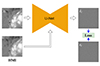 |
Fig. 1. Workflow for the training of DeepHMI in the reverse diffusion process. We send a randomly selected image xt, together with an HMI LOS magnetogram, to U-Net, where the HMI LOS magnetogram is temporally and spatially aligned with the corresponding GST/NIRIS LOS magnetogram x0. U-Net predicts the noise |

During testing/inference, we started with a random Gaussian noise  and sent as input
  , together with an HMI LOS magnetogram that was treated as a conditional image, to the trained DeepHMI model. The conditional image was used to guide the model inference. Through an iterative algorithm, the model transformed
  to an image
  that approximated the target image x0, where x0 is the corresponding GST/NIRIS LOS magnetogram that is temporally and spatially aligned with the input HMI LOS magnetogram. Initially
  . In each iteration, the model predicts
  and obtains
  by denoising
  using
using  . This
  becomes
  in the next iteration. In the end, DeepHMI produces
  as the output. Figure 2 explains the testing of DeepHMI. Thus, the input HMI LOS magnetogram is transformed into the enhanced/super-resolved image
  , which has a resolution similar to x0. In other words, the HMI LOS magnetogram is enhanced to the corresponding GST/NIRIS LOS magnetogram.
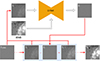 |
Fig. 2. Workflow for the testing of DeepHMI. This is an iterative method. See text for the details of the method. |
4. Results
4.1. Evaluation metrics
We conducted a series of experiments to evaluate the performance of DeepHMI. The metrics we used in the experiments include the structural similarity index measure (SSIM), the Pearson's correlation coefficient (PCC), the peak signal-to-noise ratio (PSNR), and the learned perceptual image patch similarity (LPIPS). The SSIM quantifies the degree of similarity between two images A and B, where A represents an enhanced/super-resolved HMI magnetogram image and B represents the corresponding GST/NIRIS magnetogram image (target image) in the test set. PCC indicates the correlation between A and B. PNSR also quantifies the similarity between A and B, where a high PSNR value implies that A, representing the processed image, is only very little distorted compared to the target image B. Both SSIM and PCC range from −1 to 1, and PSNR ranges from 0 to ∞. The higher the metric values, the greater the likelihood that A and B are similar. These metrics are widely used in super-resolution of solar images (Dou et al. 2024; Qin et al. 2024; Song et al. 2024; Xu et al. 2024). LPIPS quantifies the perceptual difference between A and B (Song et al. 2024). LPIPS ranges from 0 to 1. The smaller LPIPS, the greater the similarity of A to B.
4.2. Performance assessment and comparison
Figure 3 presents the average metric values obtained by DeepHMI on all testing data in the test set where the PSNR values are scaled by dividing the original values by 100. The figure also compares DeepHMI with a baseline method, namely the bicubic interpolation method, which is commonly used in solar image super-resolution (Rahman et al. 2020; Muñoz-Jaramillo et al. 2024; Xu et al. 2024). Figure 3a (Figure 3b, respectively) shows the results for super-resolving HMI transverse (LOS, respectively) magnetograms in the test set. For the enhanced HMI transverse magnetograms, the bicubic method achieves an SSIM of 0.617, a PCC of 0.629, a PSNR of 22.6, and an LPIPS of 0.651 on average. DeepHMI achieves an SSIM of 0.670, a PCC of 0.708, a PSNR of 25.7, and an LPIPS of 0.547 on average. DeepHMI improves the bicubic method by 8.6% in SSIM, 12.6% in PCC, 13.7% in PSNR, and 16.0% in LPIPS. For the enhanced HMI LOS magnetograms, the bicubic method achieves an SSIM of 0.693, a PCC of 0.756, a PSNR of 28.1, and an LPIPS of 0.417 on average. DeepHMI achieves an SSIM of 0.735, a PCC of 0.817, a PSNR of 31.0, and an LPIPS of 0.375 on average. DeepHMI improves the bicubic method by 6.1% in SSIM, 8.1% in PCC, 10.3% in PSNR, and 10.1% in LPIPS. Although DeepHMI only surpasses bicubic by a modest margin according to these metrics, it is important to note that the bicubic interpolation merely fills the resolution gap by assigning fixed values based on nearby pixels. However, DeepHMI can capture finer details and variations in the data, as demonstrated in the case study below.
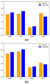 |
Fig. 3. Performance assessment and comparison of DeepHMI and the bicubic method. (a) Results for super-resolving HMI transverse magnetograms. (b) Results for super-resolving HMI LOS magnetograms. The PSNR values are scaled by dividing the original values by 100. DeepHMI performs better than the bicubic method in all metrics. |
4.3. Case study on active region NOAA 12371
In this section, we present a case study in which we used DeepHMI to enhance HMI magnetograms that were collected from the active region NOAA 12371 at 16:48:00 UT on 22 June 2015. We first present results for the HMI transverse magnetogram on the AR, which are followed by results for the HMI LOS magnetogram on the same AR. These magnetogram images were taken from the test set, which is separate from the training set.
4.3.1. Results for the super-resolution of the HMI transverse magnetogram
Figure 4 shows from left to right the original HMI transverse magnetogram, the enhanced transverse magnetogram generated/predicted by DeepHMI, and the corresponding GST/NIRIS transverse magnetogram of AR 12371. The enhanced transverse magnetogram is much clearer and shows more details than the HMI transverse magnetogram. Moreover, the magnetic field strength of the enhanced transverse magnetogram is more similar to that of the GST/NIRIS transverse magnetogram than the magnetic field strength of the HMI transverse magnetogram. Quantitatively, when the HMI transverse magnetogram is compared with the GST/NIRIS transverse magnetogram, we obtain an SSIM of 0.657, a PCC of 0.847, a PSNR of 19.1, and an LPIPS of 0.656. When the enhanced transverse magnetogram is compared with the GST/NIRIS transverse magnetogram, we obtain an SSIM of 0.691, a PCC of 0.883, a PSNR of 21.4, and an LPIPS of 0.603. In terms of the metric values, the enhanced transverse magnetogram is also more similar to the GST/NIRIS transverse magnetogram than the HMI transverse magnetogram.
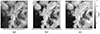 |
Fig. 4. Comparison of the HMI transverse magnetogram, the DeepHMI-enhanced transverse magnetogram, and the corresponding GST/NIRIS transverse magnetogram of AR 12371 at 16:48:00 UT on 22 June 2015. (a) HMI transverse magnetogram. (b) Enhanced HMI transverse magnetogram. (c) GST/NIRIS transverse magnetogram. |
Figure 5a (Figure 5b, respectively) shows the scatterplot of the HMI transverse magnetogram versus the GST/NIRIS transverse magnetogram (the enhanced transverse magnetogram versus the GST/NIRIS transverse magnetogram, respectively). The diagonal black line has a slope of one, and the dashed regression line has a slope of 0.65 (0.89, respectively) in Figure 5a (Figure 5b, respectively). Figure 5c presents histograms showing the number of pixels as a function of the magnetic field strength for the three magnetograms. In terms of the distribution of magnetic field strengths of pixels, the enhanced transverse magnetogram is again more similar to the GST/NIRIS transverse magnetogram than the HMI transverse magnetogram.
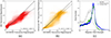 |
Fig. 5. Scatterplots and histograms obtained when the HMI transverse magnetogram of AR 12371 at 16:48:00 UT on 22 June 2015 is super-resolved. (a) Scatterplot of the HMI transverse magnetogram vs. the corresponding GST/NIRIS transverse magnetogram. (b) Scatterplot of the enhanced HMI transverse magnetogram vs. the corresponding GST/NIRIS transverse magnetogram. (c) Histograms of the three magnetograms mentioned above. |
Figures 6a, b, and c show the 2D power spectrum of the HMI transverse magnetogram, the enhanced transverse magnetogram, and the GST/NIRIS transverse magnetogram, respectively, in Figure 4. Figure 6d shows the azimuthally averaged power spectrum of the three transverse magnetograms. The radii of the three circles in the 2D power spectrum in Figures 6a, b, and c represent spatial frequencies of 1.5 Mm−1, 3.0 Mm−1, and 4.5 Mm−1, respectively. The number of pixels in the azimuthally averaged power spectrum in Figure 6d equals 1/(0.06×f), where f is the spatial frequency (Wang et al. 2017; Jing et al. 2023; Yurchyshyn et al. 2024). Thus, the radii of the three circles in the 2D power spectrum in Figures 6a, b, and c correspond to the three dashed red lines in the azimuthally averaged power spectrum in Figure 6d at spatial scales of 1/(0.06×1.5) = 11.1 pixels, 1/(0.06×3.0) = 5.5 pixels, and 1/(0.06×4.5) = 3.7 pixels, respectively.
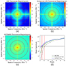 |
Fig. 6. 2D power spectra and azimuthally averaged power spectrum of the magnetograms in Figure 4. (a) 2D power spectrum of the HMI transverse magnetogram. (b) 2D power spectrum of the enhanced HMI transverse magnetogram. (c) 2D power spectrum of the corresponding GST/NIRIS transverse magnetogram. (d) Azimuthally averaged power spectrum of the three magnetograms mentioned above. |
We adopted a power spectrum threshold of 109, represented by the dashed black line, in Figure 6d. We chose this threshold because the differences between the three transverse magnetograms, represented by the three colored curves in Figure 6d, are most apparent with respect to this threshold. The intersections of the dashed black line and the three colored curves in Figure 6d show that the threshold of 109 corresponds to 11.1, 6.8, and 3.7 pixels in the HMI transverse magnetogram, the enhanced transverse magnetogram and the GST/NIRIS transverse magnetogram, respectively. The 11.1, 6.8, and 3.7 pixels correspond to spatial frequencies of 1/(0.06×11.1) = 1.5 Mm−1, 1/(0.06×6.8) = 2.4 Mm−1, and 1/(0.06×3.7) = 4.5 Mm−1, respectively.
In Figures 6a, b, and c, a spatial frequency of zero represents the scale over a full test image with the highest power. When the spatial frequency increases, the power spectrum decreases as the pixel colors change from red to green/blue. The HMI transverse magnetogram, the enhanced transverse magnetogram, and the GST/NIRIS transverse magnetogram achieve the same information content with respect to the power spectrum threshold of 109 at spatial frequencies of 1.5 Mm−1, 2.4 Mm−1 and 4.5 Mm−1, respectively, with mostly green/blue pixel colors in Figures 6a, b and c, respectively. This result suggests that a small area with 3.7 × 3.7 pixels in the GST/NIRIS transverse magnetogram image has the same amount of information as the much larger area with 11.1 × 11.1 pixels in the HMI transverse magnetogram image.
4.3.2. Results for the super-resolution of the HMI LOS magnetogram
Figures 7a, b, and c show the original HMI LOS magnetogram, the enhanced LOS magnetogram generated/predicted by DeepHMI, and the corresponding GST/NIRIS LOS magnetogram of AR 12371. When the HMI LOS magnetogram is compared with the GST/NIRIS LOS magnetogram, we obtain an SSIM of 0.639, a PCC of 0.902, a PSNR of 22.1, and an LPIPS of 0.483. When the enhanced LOS magnetogram is compared with the GST/NIRIS LOS magnetogram, we obtain an SSIM of 0.668, a PCC of 0.924, a PSNR of 23.2, and an LPIPS of 0.446. In terms of the metric values, the enhanced LOS magnetogram is more similar to the GST/NIRIS LOS magnetogram than the HMI LOS magnetogram.
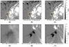 |
Fig. 7. Comparison of the HMI LOS magnetogram, the DeepHMI-enhanced LOS magnetogram, and the corresponding GST/NIRIS LOS magnetogram of AR 12371 at 16:48:00 UT on 22 June 2015. (a) HMI LOS magnetogram. (b) Enhanced HMI LOS magnetogram. (c) GST/NIRIS LOS magnetogram. (d) FOV of the region highlighted by the yellow box in (a). (e) FOV of the region highlighted by the yellow box in (b). (f) FOV of the region highlighted by the yellow box in (c). |
Figures 7d, e, and f present the field of view (FOV) of the region highlighted by the yellow box in Figures 7a, b, and c, respectively. The negative-polarity region in the center of the FOV of the HMI LOS data appears to be fuzzy. In contrast, two small negative-polarity regions in the FOV of the GST/NIRIS LOS data are clearly visible. In the FOV of the enhanced LOS data, the negative-polarity region becomes two small negative-polarity regions, similar to those in the GST/NIRIS LOS data. This indicates that DeepHMI is capable of recognizing intricate magnetic features that are not captured in the HMI LOS observation, while improving the resolution of the HMI LOS data.
Figure 8a (Figure 8b, respectively) shows the scatterplot of the HMI LOS magnetogram versus the GST/NIRIS LOS magnetogram (the enhanced LOS magnetogram versus the GST/NIRIS LOS magnetogram, respectively). The diagonal black line has a slope of 1 and the dashed regression line has a slope of 0.89 (0.96, respectively) in Figure 8a (Figure 8b, respectively). Figure 8c presents histograms showing the number of pixels as a function of the magnetic field strength for the three magnetograms. In terms of the distribution of magnetic field strengths of pixels, the enhanced LOS magnetogram is more similar to the GST/NIRIS LOS magnetogram than the HMI LOS magnetogram.
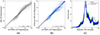 |
Fig. 8. Scatterplots and histograms obtained when super-resolving the HMI LOS magnetogram of AR 12371 at 16:48:00 UT on 22 June 2015. (a) Scatterplot of the HMI LOS magnetogram vs. the corresponding GST/NIRIS LOS magnetogram. (b) Scatterplot of the enhanced HMI LOS magnetogram vs. the corresponding GST/NIRIS LOS magnetogram. (c) Histograms of the three magnetograms mentioned above. |
Moreover, we note that in Figure 5c, the magnetic field strengths of many pixels in the strong magnetic field region of the HMI transverse magnetogram (GST/NIRIS transverse magnetogram, respectively) fall within the range between 800 and 1000 Gauss (between 1100 and 1200 Gauss, respectively). By contrast, in Figure 8c, the magnetic field strengths of many pixels in the strong magnetic field region of the HMI LOS magnetogram (GST/NIRIS LOS magnetogram, respectively) fall within the range between 1100 and 1300 Gauss (between 1000 and 1100 Gauss, respectively). Combing Figures 5c and 8c, we show that the low-resolution HMI assigns many strong magnetic elements to the LOS direction, while the high-resolution GST/NIRIS assigns many strong magnetic elements to the transverse direction. When the HMI magnetograms are enhanced, DeepHMI not only improves the resolutions of the HMI magnetograms but also shifts strong magnetic elements from the LOS component to the transverse component, with a distribution similar to that in the GST/NIRIS data.
Figures 9a, b, and c show the 2D power spectrum of the HMI LOS magnetogram, the enhanced LOS magnetogram, and the GST/NIRIS LOS magnetogram, respectively, in Figure 7. Figure 9d shows the azimuthally averaged power spectrum of the three magnetograms. The three circles in Figures 9a, b, c, the three dashed red lines and the power spectrum threshold of 109, represented by the dashed black line, in Figure 9d are interpreted similarly to those of Figure 6. The HMI LOS magnetogram, the enhanced LOS magnetogram and the GST/NIRIS LOS magnetogram achieve the same information content with respect to the power spectrum threshold of 109 at the spatial frequency of 1.5 Mm−1, 2.5 Mm−1, and 4.0 Mm−1, respectively, with mostly green/blue pixel colors in Figures 9a, b, and c, respectively. The spatial frequencies of 1.5 Mm−1, 2.5 Mm−1, and 4.0 Mm−1 correspond to areas containing approximately 11.1 × 11.1 pixels, 6.6 × 6.6 pixels, and 4.2 × 4.2 pixels in the HMI LOS magnetogram, the enhanced LOS magnetogram, and the GST/NIRIS LOS magnetogram, respectively. This result suggests that the small area with 4.2 × 4.2 pixels in the GST/NIRIS LOS magnetogram image has the same amount of information as the much larger area with 11.1 × 11.1 pixels in the HMI LOS magnetogram image.
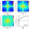 |
Fig. 9. 2D power spectrum and azimuthally averaged power spectrum of the magnetograms in Figure 7. (a) 2D power spectrum of the HMI LOS magnetogram. (b) 2D power spectrum of the enhanced HMI LOS magnetogram. (c) 2D power spectrum of the corresponding GST/NIRIS LOS magnetogram. (d) Azimuthally averaged power spectrum of the three magnetograms mentioned above. |
5. Discussion and conclusion
We proposed DeepHMI, a novel deep-learning model to upgrade SDO/HMI transverse and LOS magnetograms of solar active regions to the resolution of GST/NIRIS data. Our experimental results showed that the proposed model outperforms the commonly used bicubic interpolation method in terms of four metrics (SSIM, PCC, PSNR and, LPIPS). In addition, we presented a case study on AR 12371, in which the enhanced super-resolved HMI magnetogram reveals finer details in the transverse and LOS components, with the LOS component appropriately converted into the transverse component, closely aligning with the high-resolution GST/NIRIS data. A quantitative analysis further validated the improvement in the spatial resolution of the HMI data and highlighted that our model is effective in capturing and enhancing nuanced magnetic field details at small spatial scales. On the basis of these results, we conclude that DeepHMI is a useful tool for enhancing the HMI transverse and LOS magnetograms of solar ARs.
Another component of a vector magnetogram is the azimuth angle, for which we also conducted super-resolution experiments. Figure 10 shows from left to right the original HMI azimuth angle, the enhanced azimuth angle generated/predicted by DeepHMI, and the corresponding GST/NIRIS azimuth angle of AR 12371 at 16:48:00 UT on 22 June 2015. The uncertainties of HMI transverse magnetograms are approximately 300 Gauss, and the uncertainties of HMI LOS magnetograms are approximately 30 Gauss (Tadesse et al. 2013). Therefore, we masked the pixels of the azimuth angle in white, where the corresponding transverse field strength is weaker than 300 Gauss and the LOS field strength is weaker than 30 Gauss. Figure 10 shows that DeepHMI enhances the resolution of the azimuth angle, although the enhancement is not as strong as the enhancements obtained by super-resolving the transverse and LOS magnetograms. This occurs in part due to uncertainties in the azimuth angle calculations (Tadesse et al. 2013; Wiegelmann et al. 2014), and in part due to atmospheric effects on the ground-based GST/NIRIS instrument.
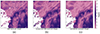 |
Fig. 10. Comparison of the HMI azimuth angle, the DeepHMI-enhanced azimuth angle, and the corresponding GST/NIRIS azimuth angle from AR 12371 at 16:48:00 UT on 22 June 2015. (a) HMI azimuth angle. (b) Enhanced HMI azimuth angle. (c) GST/NIRIS azimuth angle. |
Figure 11a (Figure 11b, respectively) shows the scatterplot of the HMI azimuth angle versus the GST/NIRIS azimuth angle (the enhanced azimuth angle versus the GST/NIRIS azimuth angle, respectively). The diagonal black line has a slope of 1, and the dashed regression line has a slope of 0.45 (0.47, respectively) in Figure 11a (Figure 11b, respectively). The HMI magnetograms and the NIRIS magnetograms used in this study were obtained through Milne-Eddington inversion, which limits their azimuth angles to between 0° and 180° (Orozco Suárez et al. 2010). In realty, the azimuth angles are between 0° and 360°. Therefore, pixels whose azimuth angles are near 0°, 180°, and 360° are clustered at 0° and 180° in Figure 11. The pixel-value distribution of the enhanced azimuth angle matches that of the GST/NIRIS azimuth angle better than that of the HMI azimuth angle. Figure 11a shows that the slope of the regression line is quite different from that of the diagonal line due to the uncertainties in the data. DeepHMI can enhance the resolution of the azimuth angle data, but it is difficult to eliminate the data uncertainties combined with atmospheric effects in this component. This is an inherent limitation in super-resolving the azimuth angle data collected by HMI using GST/NIRIS data.
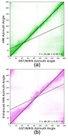 |
Fig. 11. Scatterplots obtained when super-resolving the HMI azimuth angle of AR 12371 at 16:48:00 UT on 22 June 2015. (a) Scatterplot of the HMI azimuth angle vs. the corresponding GST/NIRIS azimuth angle. (b) Scatterplot of the enhanced HMI azimuth angle vs. the corresponding GST/NIRIS azimuth angle. |
Acknowledgments
The authors appreciate the use of data from SDO and BBSO. SDO is a NASA mission. The BBSO operation is supported by NJIT and U.S. NSF grant AGS-1821294. The GST operation is partly supported by the Korea Astronomy and Space Science Institute and Seoul National University. Y. X. acknowledges support from NSF grants AGS-2228996 and AGS-2229064. Q. L. acknowledges support from NASA grants 80NSSC24K0548 and 80NSSC24M0174. J. W. and H. W. acknowledge support from NSF grants AGS-2149748, AGS-2228996, OAC-2320147, and NASA grants 80NSSC24K0548, 80NSSC24K0843, and 80NSSC24M0174.
Available at http://jsoc.stanford.edu/
References
- Amar, E., & Ben-Shahar, O. 2024, ApJS, 271, 29 [Google Scholar]
- Bobra, M. G., & Couvidat, S. 2015, ApJ, 798, 135 [Google Scholar]
- Deng, J., Song, W., Liu, D., et al. 2021, ApJ, 923, 76 [CrossRef] [Google Scholar]
- Díaz Baso, C. J., & Asensio Ramos, A. 2018, A&A, 614, A5 [NASA ADS] [CrossRef] [EDP Sciences] [Google Scholar]
- Díaz Baso, C. J., de la Cruz Rodríguez, J., & Danilovic, S. 2019, A&A, 629, A99 [NASA ADS] [CrossRef] [EDP Sciences] [Google Scholar]
- Dou, F., Xu, L., Zhao, D., & Ren, Z. 2024, ApJS, 271, 9 [Google Scholar]
- Eren, S., Kilcik, A., Atay, T., et al. 2017, MNRAS, 465, 68 [Google Scholar]
- Falk, T., Mai, D., Bensch, R., et al. 2019, Nature Methods, 16, 67 [CrossRef] [PubMed] [Google Scholar]
- Habeeb, M. S., Aydin, B., Ahmadzadeh, A., Georgoulis, M. K., & Angryk, R. A. 2020, IEEE International Conference on Big Data (IEEE BigData 2020), 4200–4207 [Google Scholar]
- Higgins, R. E. L., Fouhey, D. F., Antiochos, S. K., et al. 2022, ApJS, 259, 24 [Google Scholar]
- Ho, J., Jain, A., & Abbeel, P. 2020, in Advances in Neural Information Processing Systems, 33, 6840 [Google Scholar]
- Jiang, H., Li, Q., Xu, Y., et al. 2022, ApJ, 939, 66 [Google Scholar]
- Jin, C., Zhou, G., Ruan, G., et al. 2023, ApJ, 942, L3 [CrossRef] [Google Scholar]
- Jing, J., Liu, N., Lee, J., et al. 2023, ApJ, 952, 40 [Google Scholar]
- Li, Q., Deng, N., Jing, J., Liu, C., & Wang, H. 2019, ApJ, 876, 129 [NASA ADS] [CrossRef] [Google Scholar]
- Liu, H., Liu, C., Wang, J. T. L., & Wang, H. 2020, ApJ, 890, 12 [Google Scholar]
- Muñoz-Jaramillo, A., Jungbluth, A., Gitiaux, X., et al. 2024, ApJS, 271, 46 [Google Scholar]
- Nishizuka, N., Sugiura, K., Kubo, Y., et al. 2017, ApJ, 835, 156 [NASA ADS] [CrossRef] [Google Scholar]
- Orozco Suárez, D., Bellot Rubio, L. R., Vögler, A., & Del Toro Iniesta, J. C. 2010, A&A, 518, A2 [Google Scholar]
- Pesnell, W. D., Thompson, B. J., & Chamberlin, P. C. 2012, Sol. Phys., 275, 3 [Google Scholar]
- Qin, Y., Ji, K. -F., Liu, H., & Yu, X. -G. 2024, Research in Astronomy and Astrophysics, 24, 065029 [Google Scholar]
- Rahman, S., Moon, Y. -J., Park, E., et al. 2020, ApJ, 897, L32 [NASA ADS] [CrossRef] [Google Scholar]
- Ramunno, F. P., Hackstein, S., Kinakh, V., et al. 2024, A&A, 686, A285 [NASA ADS] [CrossRef] [EDP Sciences] [Google Scholar]
- Schou, J., Scherrer, P. H., Bush, R. I., et al. 2012, Sol. Phys., 275, 229 [Google Scholar]
- Schrijver, C. J. 2007, ApJ, 655, L117 [Google Scholar]
- Schrijver, C. J. 2016, ApJ, 820, 103 [Google Scholar]
- Shan, J., Zhang, H., Lu, L., et al. 2024, ApJS, 272, 18 [Google Scholar]
- Song, H., Tan, C., Jing, J., et al. 2009, Sol. Phys., 254, 101 [NASA ADS] [CrossRef] [Google Scholar]
- Song, W., Ma, W., Ma, Y., Zhao, X., & Lin, G. 2022, ApJS, 263, 25 [NASA ADS] [CrossRef] [Google Scholar]
- Song, W., Ma, Y., Sun, H., Zhao, X., & Lin, G. 2024, A&A, 686, A272 [NASA ADS] [CrossRef] [EDP Sciences] [Google Scholar]
- Tadesse, T., Wiegelmann, T., Inhester, B., et al. 2013, A&A, 550, A14 [NASA ADS] [CrossRef] [EDP Sciences] [Google Scholar]
- Voleti, V., Jolicoeur-Martineau, A., & Pal, C. 2022, in Advances in Neural Information Processing Systems, 35, 23371 [Google Scholar]
- Wang, H., Liu, C., Ahn, K., et al. 2017, Nature Astronomy, 1, 0085 [Google Scholar]
- Wang, R., Fouhey, D. F., Higgins, R. E. L., et al. 2024, ApJ, 970, 168 [Google Scholar]
- Welsch, B. T., Li, Y., Schuck, P. W., & Fisher, G. H. 2009, ApJ, 705, 821 [NASA ADS] [CrossRef] [Google Scholar]
- Wiegelmann, T., Thalmann, J. K., & Solanki, S. K. 2014, A&ARv, 22, 78 [Google Scholar]
- Xu, C., Wang, J. T. L., Wang, H., et al. 2024, Sol. Phys., 299, 36 [Google Scholar]
- Yang, P., Bai, H., Zhao, L., et al. 2023, A&A, 677, A121 [NASA ADS] [CrossRef] [EDP Sciences] [Google Scholar]
- Yurchyshyn, V., Schmidt, A., Wang, J., et al. 2024, ApJ, 961, 79 [Google Scholar]
- Zhang, J., Tian, H., Solanki, S. K., et al. 2018, ApJ, 865, 29 [Google Scholar]
- Zhao, J., Yu, F., Zhu, X., et al. 2024, ApJ, 973, 33 [Google Scholar]
All Figures
|
Fig. 1. Workflow for the training of DeepHMI in the reverse diffusion process. We send a randomly selected image xt, together with an HMI LOS magnetogram, to U-Net, where the HMI LOS magnetogram is temporally and spatially aligned with the corresponding GST/NIRIS LOS magnetogram x0. U-Net predicts the noise |
| In the text | |
|
Fig. 2. Workflow for the testing of DeepHMI. This is an iterative method. See text for the details of the method. |
| In the text | |
|
Fig. 3. Performance assessment and comparison of DeepHMI and the bicubic method. (a) Results for super-resolving HMI transverse magnetograms. (b) Results for super-resolving HMI LOS magnetograms. The PSNR values are scaled by dividing the original values by 100. DeepHMI performs better than the bicubic method in all metrics. |
| In the text | |
|
Fig. 4. Comparison of the HMI transverse magnetogram, the DeepHMI-enhanced transverse magnetogram, and the corresponding GST/NIRIS transverse magnetogram of AR 12371 at 16:48:00 UT on 22 June 2015. (a) HMI transverse magnetogram. (b) Enhanced HMI transverse magnetogram. (c) GST/NIRIS transverse magnetogram. |
| In the text | |
|
Fig. 5. Scatterplots and histograms obtained when the HMI transverse magnetogram of AR 12371 at 16:48:00 UT on 22 June 2015 is super-resolved. (a) Scatterplot of the HMI transverse magnetogram vs. the corresponding GST/NIRIS transverse magnetogram. (b) Scatterplot of the enhanced HMI transverse magnetogram vs. the corresponding GST/NIRIS transverse magnetogram. (c) Histograms of the three magnetograms mentioned above. |
| In the text | |
|
Fig. 6. 2D power spectra and azimuthally averaged power spectrum of the magnetograms in Figure 4. (a) 2D power spectrum of the HMI transverse magnetogram. (b) 2D power spectrum of the enhanced HMI transverse magnetogram. (c) 2D power spectrum of the corresponding GST/NIRIS transverse magnetogram. (d) Azimuthally averaged power spectrum of the three magnetograms mentioned above. |
| In the text | |
|
Fig. 7. Comparison of the HMI LOS magnetogram, the DeepHMI-enhanced LOS magnetogram, and the corresponding GST/NIRIS LOS magnetogram of AR 12371 at 16:48:00 UT on 22 June 2015. (a) HMI LOS magnetogram. (b) Enhanced HMI LOS magnetogram. (c) GST/NIRIS LOS magnetogram. (d) FOV of the region highlighted by the yellow box in (a). (e) FOV of the region highlighted by the yellow box in (b). (f) FOV of the region highlighted by the yellow box in (c). |
| In the text | |
|
Fig. 8. Scatterplots and histograms obtained when super-resolving the HMI LOS magnetogram of AR 12371 at 16:48:00 UT on 22 June 2015. (a) Scatterplot of the HMI LOS magnetogram vs. the corresponding GST/NIRIS LOS magnetogram. (b) Scatterplot of the enhanced HMI LOS magnetogram vs. the corresponding GST/NIRIS LOS magnetogram. (c) Histograms of the three magnetograms mentioned above. |
| In the text | |
|
Fig. 9. 2D power spectrum and azimuthally averaged power spectrum of the magnetograms in Figure 7. (a) 2D power spectrum of the HMI LOS magnetogram. (b) 2D power spectrum of the enhanced HMI LOS magnetogram. (c) 2D power spectrum of the corresponding GST/NIRIS LOS magnetogram. (d) Azimuthally averaged power spectrum of the three magnetograms mentioned above. |
| In the text | |
|
Fig. 10. Comparison of the HMI azimuth angle, the DeepHMI-enhanced azimuth angle, and the corresponding GST/NIRIS azimuth angle from AR 12371 at 16:48:00 UT on 22 June 2015. (a) HMI azimuth angle. (b) Enhanced HMI azimuth angle. (c) GST/NIRIS azimuth angle. |
| In the text | |
|
Fig. 11. Scatterplots obtained when super-resolving the HMI azimuth angle of AR 12371 at 16:48:00 UT on 22 June 2015. (a) Scatterplot of the HMI azimuth angle vs. the corresponding GST/NIRIS azimuth angle. (b) Scatterplot of the enhanced HMI azimuth angle vs. the corresponding GST/NIRIS azimuth angle. |
| In the text | |
Current usage metrics show cumulative count of Article Views (full-text article views including HTML views, PDF and ePub downloads, according to the available data) and Abstracts Views on Vision4Press platform.
Data correspond to usage on the plateform after 2015. The current usage metrics is available 48-96 hours after online publication and is updated daily on week days.
Initial download of the metrics may take a while.