| Issue |
A&A
Volume 686, June 2024
|
|
|---|---|---|
| Article Number | A272 | |
| Number of page(s) | 13 | |
| Section | Numerical methods and codes | |
| DOI | https://doi.org/10.1051/0004-6361/202349100 | |
| Published online | 21 June 2024 | |
Improving the spatial resolution of solar images using super-resolution diffusion generative adversarial networks★
1
School of Information Engineering, Minzu University of China,
Beijing
100081, PR China
e-mail: songwei@muc.edu.cn; maying_ya@163.com
2
Key Laboratory of Solar Activity, Chinese Academy of Sciences (KLSA, CAS),
Beijing
100081, PR China
3
National Language Resource Monitoring and Research Center of Minority Languages, Minzu University of China,
Beijing
100081, PR China
4
Key Laboratory of Ethnic Language Intelligent Analysis and Security Governance of MOE, Minzu University of China,
Beijing
100081, PR China
5
National Astronomical Observatories, Chinese Academy of Sciences (NAOC, CAS),
Beijing
100081, PR China
Received:
25
December
2023
Accepted:
21
March
2024
Context. High-spatial-resolution solar images contribute to the study of small-scale structures on the Sun. The Helioseismic and Magnetic Imager (HMI) conducts continuous full-disk observations of the Sun at a fixed cadence, accumulating a wealth of observational data. However, the spatial resolution of HMI images is not sufficient to analyze the small-scale structures of solar activity.
Aims. We present a new super-resolution (SR) method based on generative adversarial networks (GANs) and denoising diffusion probabilistic models (DDPMs) that can increase the spatial resolution of HMI images by a factor four.
Methods. We propose a method called super-resolution diffusion GANs (SDGAN), which combines GANs and DDPMs for the SR reconstruction of HMI images. SDGAN progressively maps low-resolution (LR) images to high-resolution (HR) images through a conditional denoising process. It employs conditional GANs to simulate the denoising distribution and optimizes model results using nonsaturating adversarial loss and perceptual loss. This approach enables fast and high-quality reconstruction of solar images.
Results. We used high-spatial-resolution images from the Goode Solar Telescope (GST) as HR images and created a data set consisting of paired images from HMI and GST. We then used this data set to train SDGAN for the purpose of reconstructing HMI images with four times the original spatial resolution. The experimental results demonstrate that SDGAN can obtain high-quality HMI reconstructed images with just four denoising steps.
Key words: methods: data analysis / techniques: image processing / Sun: activity / Sun: photosphere
The movie is available at https://www.aanda.org. The code and test set are available at https://github.com/laboratory616/SDGAN
© The Authors 2024
 Open Access article, published by EDP Sciences, under the terms of the Creative Commons Attribution License (https://creativecommons.org/licenses/by/4.0), which permits unrestricted use, distribution, and reproduction in any medium, provided the original work is properly cited.
This article is published in open access under the Subscribe to Open model. Subscribe to A&A to support open access publication.
1 Introduction
Observing and studying solar activity is of great significance to humanity (Schwenn 2006). Understanding and predicting the impact of solar activity on the Earth’s environment remains one of the main research topics at the forefront of solar physics. The solar active regions have a wide range of large-scale and small-scale structures, and the small-scale structures are close to the spatial resolution of observational instruments (Nelson et al. 2013). It is generally believed that small-scale solar-activity phenomena are intrinsically related to large-scale phenomena. Therefore, high-spatial-resolution solar data are beneficial for further research into fundamental issues in solar physics.
The Solar Dynamics Observatory (SDO; Pesnell et al. 2012) was launched by NASA in 2010. The Helioseismic and Magnetic Imager (HMI; Scherrer et al. 2012) is one of three instruments on board the SDO. HMI is primarily designed to study the origin of solar variability and to characterize and understand the Sun’s interior and the various components of magnetic activity. For more than a decade, HMI has been continuously observing the full solar disk every 45 s (or every 720s for a better signal-to-noise ratio). HMI has accumulated a large amount of historical observational data. HMI provides 0.504″ resolution solar images of dopplergrams, continuum intensity images, and vector magnetograms. As a space-based telescope, HMI is not affected by the Earth’s atmosphere. The spatial resolution of HMI images is limited by the diffraction limit of the telescope. The trade-off between full-disk observations and spatial resolution means that HMI images are insufficient for analyzing small-scale structures in the solar atmosphere (Baso & Ramos 2018). Improving the spatial resolution of HMI images can provide higher-resolution and richer solar image data for research in astronomy and solar physics, enabling better studies of the morphological and dynamic properties of solar penumbral filaments, granules, and sunspots. Using super-resolution (SR) methods to improve the spatial resolution of HMI images requires the selection of appropriate high-resolution (HR) observation images.
The Goode Solar Telescope (GST) of the Big Bear Solar Observatory (BBSO) is a large-aperture ground-based solar telescope (Goode & Cao 2012). GST observes the Sun with diffraction-limited resolution at visible and near-infrared wavelengths to investigate the solar photosphere and chromosphere. GST uses a high-order adaptive optics (AO) system with 308 subapertures to provide high-order correction of atmospheric distortion (Shumko et al. 2014). Additionally, it utilizes post facto speckle image reconstruction techniques to achieve diffraction-limited imaging of the solar atmosphere (Su et al. 2018). TiO and Hα images are acquired through GST observations. With a spatial resolution of 0.034″, GST images exhibit high spatial resolution and observational accuracy and can effectively capture small-scale solar structures, providing rich details in the observations. However, GST faces limitations imposed by atmospheric turbulence and day-night changes, preventing long-term continuous solar observation. Additionally, the acquired GST images have a restricted field of view, limiting their observation to local solar activity. The structures of solar images observed by GST and HMI are similar, and the spatial resolution of GST images is higher than that of HMI images, which can provide more detailed information for HMI images.
Super-resolution is a classic problem in the field of computer vision, with the aim being to recover an HR image from one or more observed low-resolution (LR) images (Park et al. 2003; Dong et al. 2015; Rahman et al. 2020). For massive data, traditional SR methods, such as interpolation techniques, are no longer sufficient to meet modern requirements. SR methods based on deep learning attempt to learn the internal relationship between LR and HR images from the given data set, and then achieve SR reconstruction of LR images based on the learned mapping relationship. Improving the quality of observational data through deep learning-based methods has gradually become an important method for data analysis and processing in solar physics research (Yang et al. 2023). Different types of deep learning models have been applied to the task of SR reconstruction of solar images. Baso & Ramos (2018) successfully applied a deep convolutional neural network (CNN) to the deconvolution and SR of solar images for the first time, and the reconstructed images can simulate the results observed by a telescope with a diffraction limit twice the diameter of HMI.
Generative adversarial networks (GANs; Goodfellow et al. 2020) generate realistic data samples through adversarial training of generator and discriminator, and are widely used in solar image SR reconstruction (Jia et al. 2019; Alshehhi 2022; Yang et al. 2023). Deng et al. (2021) used the scale-invariant feature transform (SIFT; Lowe 2004) to construct precisely aligned HMI and GST image pairs, and used a neural network combining GANs and self-attention mechanisms (SAGAN) to restore the details of the solar active region, reconstructing HMI images with a spatial resolution increased by a factor four. SAGAN achieves good reconstruction results, but some of the reconstructed images have some unrealistic textures. Although GAN-based approaches have developed rapidly, and many studies are devoted to dealing with the mode collapse problem of GANs (Saxena & Cao 2021; Karras et al. 2021), this latter issue remains challenging.
Diffusion models are likelihood-based generative models that directly learns the probability density of the distribution through maximum likelihood. Inspired by equilibrium thermodynamics, diffusion models define a Markov chain that gradually adds random Gaussian noise to the data, and then learns the inverse diffusion process to construct the desired data samples from the noise. Due to the stepwise random sampling process and explicit likelihood representation, diffusion models can improve the reliability of network mapping, thereby improving the quality and diversity of samples. As powerful generative models, diffusion models obtain good results in terms of sample quality and are superior to GANs in their ability to generate images (Dhariwal & Nichol 2021; Ho et al. 2022). Diffusion models also achieve good mode coverage, indicated by high likelihood (Song et al. 2021a; Huang et al. 2021). Song et al. (2022) proposed the improved conditional denoising diffusion probability model (ICDDPM), which reconstructs HR images from LR images by learning the reverse process of adding noise to LR images. The spatial resolution of HMI images has been increased to four times the original, and the reconstruction effect is better than that of SAGAN. However, the reconstruction speed of ICDDPM for HMI images is about four times that of SAGAN. Although the image quality obtained by diffusion models is relatively good, due to the Gaussian assumption in the denoising distribution, the number of denoising steps in diffusion models ranges from hundreds to thousands (Xiao et al. 2021), resulting in slow sampling speed and requiring significant computational resources, which limits their practical application.
We regard HMI images as LR images and GST images as HR images to achieve SR reconstruction of HMI images. Inspired by denoising diffusion GANs (Xiao et al. 2021), we propose super-resolution diffusion GANs (SDGAN), which uses deep learning methods to learn the mapping relationship between HR images and LR images. SDGAN combines the ideas of GANs and denoising diffusion probabilistic models (DDPMs; Ho et al. 2020), gradually adding noise to HR images through the diffusion process, and modeling the denoising distribution through a GAN conditioned on LR images during the denoising process, removing noise from LR images in large steps, thereby achieving SR reconstruction of LR images. SDGAN can achieve efficient and high-quality image reconstruction through a small number of large diffusion steps, obtaining reconstructed HMI images with four times the spatial resolution of the original images.
The remainder of this paper is organized as follows: in Sect. 2, we introduce the principle and network architecture of our proposed SDGAN model in detail. In Sect. 3, we describe the data set and training details. In Sect. 4, we present the ablation experiments of our model and show the reconstruction results of SDGAN. Additionally, we compare the results of SDGAN with those of SAGAN (Deng et al. 2021) and ICDDPM (Song et al. 2022). We present our conclusions in Sect. 5.
2 Super-resolution diffusion GANs
2.1 Diffusion process and denoising process
In the diffusion process, SDGAN gradually adds Gaussian noise to HR images, transforming the distribution of HR images into Gaussian distribution. In the denoising process, which is conditioned on LR images, the generator gradually removes noise to obtain SR reconstructed images (see Fig. 1).
Given a data point x0 sampled from the distribution q(x) of HR images, one can define a diffusion process by adding Gaussian noise, thereby generating latent variables x1…xt, xt−1,…xT that have the same dimensions as x0. We define the distribution of the diffusion process q(xt|xt−1), which adds Gaussian noise at each timestep t, according to a known variance schedule ß1,…, βT · β1,…, βT is an increasing sequence ranging from 0 to 1, which is used to control the speed of adding noise. This diffusion process can be formulated as follows:

where I represents the identity matrix with the same dimensions as xt−1 . After T steps of adding noise, the data x0 are destroyed, and the latent xT is approximately an isotropic Gaussian distribution (Nichol & Dhariwal 2021).
In order to model the denoising distribution pθ(xt−1|xt) with the Gaussian distribution, DDPMs sets ßt to a relatively small value, and T is set to 1000. This choice results in a slow sampling speed, thereby limiting the efficiency of image generation. In order to speed up model sampling and achieve efficient reconstruction, SDGAN sets T to a smaller value. The method in variance preserving stochastic differential equation (VP SDE; Song et al. 2021b) is used to calculate ßt, which allows us to ensure that the variance schedule remains unchanged and is independent of the number of diffusion steps. ßt can be calculated using the following equation:

where constants ßmax = 20 and ßmin = 0.1 are the maximum and minimum values of ß1,…, ßT respectively.
According to the properties of the Gaussian distribution, if we define αt = 1 − ßt and  , we can use the reparameterization method in a recursive manner to get:

Using Eq. (3), xt can be regarded as a linear combination of the original data x0 and random Gaussian noise ϵ ~ 𝒩(0, I), that is,  . According to the above equation and Bayes’ theorem, we can obtain the posterior probability distribution of xt−1 when x0 and xt are known:

where  .
.
In the diffusion process, SDGAN uses a small T and a large ßt sequence. In this case, the true denoising distribution q(xt−1|xt, y) becomes complex and multimodal, and cannot be modeled as a Gaussian distribution in the form of the reverse process distribution as in DDPMs. Conditional GANs can simulate complex conditional distributions in the image domain (Mirza & Osindero 2014; Ledig et al. 2017; Isola et al. 2017), and so we use the generator of the conditional GANs to model the denoising distribution pθ(xt−1|xt, y) as a non-Gaussian distribution.
The conditional generator Gθ(xt, y, t) performs gradual denoising in each denoising step to synthesize xt−1 ~ pθ (xt−1|xt, y). The generator takes the result xt of the diffusion process and t as input, with the LR image as the condition y. The diffusion level of xt varies for different t, making it challenging to directly predict xt−1 under different values of t. The posterior distribution q(xt−1|xt, x0) is a Gaussian distribution that is independent of both T and the complexity of the data distribution. Therefore, the generator of SDGAN is used to predict x′0 that has not undergone diffusion. Then according to Eq. (4), x′t−1 under the conditions of x′0 and xt is obtained through the posterior distribution q(xt−1|xt, x′0). After T iterations of the above steps, the reconstructed image  can be obtained. The discriminator Dφ (xt−1, xt, t) takes (x′t−1, xt, t) and (xt−1, xt, t) as input, respectively, and determines whether x′t−1 or xt−1 is a plausible denoised version of xt. The t in the generator and discriminator represents the transformer sinusoidal position embedding (Vaswani et al. 2017), enabling parameters to be shared across time.
Training GANs to directly sample from complex distributions can result in unstable training and suboptimal reconstruction outcomes. SDGAN simplifies the modeling process by decomposing the sampling process into multiple conditional denoising steps. Furthermore, the diffusion process can contribute to smoothing the data distribution (Lyu 2009), thereby aiding in mitigating overfitting of the discriminator to some extent. DDPM uses a Gaussian distribution to model the denois-ing distribution, leading to large sampling steps and slow sampling speed. In contrast, SDGAN utilizes conditional GANs to model the denoising distribution, allowing for the use of smaller T, and thereby reducing the sampling steps in the diffusion process and accelerating the sampling speed.
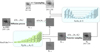 |
Fig. 1 Architecture of SDGAN. The number after n represents the number of channels in the feature map. Gθ and Dφ are the generator and discriminator modules of SDGAN, respectively. x0 and y represent HR images and LR images, respectively. |
2.2 Loss function
We optimize the parameters of the generator by minimizing the nonsaturating adversarial loss between the true denoising distribution q(xt−1|xt, y) and the estimated denoising distribution
pθ(xt−1|xt, y):
![${L_{{G_\theta }}} = {_{t,q\left( {{x_{t - 1}}\mid {x_t},y} \right),{p_\theta }\left( {{x_{t - 1}}\mid {x_t},y} \right)}}\left[ { - \log {D_\phi }\left( {x_{t - 1}^\prime ,{x_t},t} \right)} \right].$](/articles/aa/full_html/2024/06/aa49100-23/aa49100-23-eq9.png)
In addition to the adversarial loss, we also add perceptual loss between x0 and x′0 in the generator:
![${L_{{\rm{perception}}}} = {_{t,{p_\ell }\left( {{x_{t - 1}}\mid {x_t},y} \right)}}\left[ {VGG\left( {x_0^\prime } \right) - VGG\left( {{x_0}} \right)} \right]{\rm{.}}$](/articles/aa/full_html/2024/06/aa49100-23/aa49100-23-eq10.png)
The perceptual loss employs VGG19 (Simonyan & Zisserman 2015) to compute the feature maps of x′0 and x0, and then calculates the mean absolute error between their respective feature maps. Finally, the mean absolute error is added according to a certain weight to obtain the value of perceptual loss. Perceptual loss can decrease the difference between x′0 and x0 in terms of perceptual quality, improve the visual quality of the reconstructed image and the semantic consistency between the reconstructed image and the HR image.
The discriminator Dφ is trained using the nonsaturating adversarial loss with gradient penalty:
![$\matrix{ {{L_{{D_\phi }}} = \left. {{E_{t,q\left( {\left. {{x_t}} \right|{x_0}} \right.}}} \right)\left[ {{_{q\left( {{x_{t - 1}}\mid {x_t},y} \right)}}\left[ { - \log {D_\phi }\left( {{{\bf{x}}_{t - 1}},{{\bf{x}}_t},t} \right)} \right]} \right]} \hfill \cr {\,\,\,\,\,\,\,\,\,\,\,\,\,\,\, + {_{{p_\theta }\left( {{x_{t - 1}}\mid {x_t},y} \right)}}\left[ { - \log \left( {1 - {D_\phi }\left( {x_{t - 1}^\prime ,{x_t},t} \right)} \right)} \right] + {R_1},} \hfill \cr } $](/articles/aa/full_html/2024/06/aa49100-23/aa49100-23-eq11.png)
![${R_1} = \eta {_{q\left( {{x_{t - 1}}\mid {x_t},y} \right)}}\left[ {{{\left\| {{\nabla _{{x_{t - 1}}}}{D_\phi }\left( {{x_{t - 1}},{x_t},t} \right)} \right\|}^2}} \right],$](/articles/aa/full_html/2024/06/aa49100-23/aa49100-23-eq12.png)
where η is the coefficient for the regularization. A gradient penalty encourages the discriminator to remain smooth and improves the convergence of GAN training (Mescheder et al. 2018).
2.3 Network structure
The generator structure mainly refers to the design of NCSN++ (Song et al. 2021b), which is a U-Net structure (Ronneberger et al. 2015) composed of multiple attention blocks (He et al. 2016) and ResNet blocks (Vaswani et al. 2017). We use the pre-upsampling method to upsample the LR image, and then use the network to learn the representation of mapping HR images (Bashir et al. 2021). The HMI image is subjected to bicubic interpolation for 4× upsampling before being input into the generator. The size of the HMI image changes from 64 × 64 to 256 × 256.
During training, y and xt are concatenated along the channel dimension and input into the generator, and the output is the predicted x′0. When testing, conditioned on y, we start sampling from the LR image or Gaussian noise and output the predicted x′0. Gaussian noise is randomly sampled from the standard normal distribution 𝒩(0, I). Then the predicted x′t−1 is obtained through the posterior distribution q(xt−1|xt, x′0). After T iterations, the SR reconstructed image  is obtained.
The U-Net comprises a contracting path and an expanding path (see Fig. 1). The contracting path is utilized to extract abstract features from the input image, and consists of five layers. Each layer includes two convolution operations and one downsampling operation, gradually reducing the feature map size from 256 × 256 to 8 × 8. The expanding path achieves the fusion of image features from shallow and deep layers, and also consists of five layers with two convolution operations and one upsampling operation each. During the upsampling operation, skip connections are employed to concatenate the feature maps of the upsampling and downsampling according to the number of channels. We used the default settings, which entail upsampling and downsampling with anti-aliasing based on the finite impulse response (FIR; Zhang 2019) and the Swish activation function in NCSN++.
The discriminator is a CNN with ResNet blocks, which consists of a series of convolution and downsampling operations. More precisely the CNN consists of six layers, each employing LeakyReLU activation with a negative slope of 0.2. The discriminator takes the concatenation of xt and xt−1 (or x′t−1) along the channel dimension as input and outputs the probability that xt−1 or x′t−1 is a plausible denoised version of xt. To distinguish different diffusion times t, transformer sinusoidal position embeddings are utilized to encode t in both the generator and discriminator. This ensures that the model is aware of which t corresponds to the output when predicting the output in a batch.
3 Data and training
We use the full-disk continuum Intensitygram images from SDO/HMI with 0.504″ spatial resolution and a temporal cadence of 45s, and the images provided by GST/BFI with 0.034″ spatial resolution and irregular cadence. The HMI provides 4096 × 4096 pixel images, and GST provides 900 × 900 pixel images. In order to facilitate comparison with the SAGAN (Deng et al. 2021) and ICDDPM (Song et al. 2022) and verify the effectiveness of the SDGAN, we adopted the same data processing method as SAGAN and ICDDPM.
We selected SDO/HMI images from June 21, 2011 to August 24, 2020 to construct the data set, and selected the temporally closest images provided by GST/BFI as the HR image. To ensure alignment between images captured by different telescopes, we employed the SIFT method for image registration. This involves adjusting the rotation, translation, and scaling of HMI images to achieve precise alignment with GST images Deng et al. (2021). We obtained a total of 1597 image pairs spanning from 2011 to 2020. Due to limitations of hardware conditions, we performed 4× SR reconstruction of HMI images. We resized the original GST image from 900 × 900 to 552 × 552. We then applied 2D Gaussian smoothing with a (5, 5) kernel and 2σ to obtain the downsampled GST image with a spatial resolution of 0.126″. Finally, we obtained the final GST image with a size of 256 × 256 through center cropping. We cropped the HMI image to a size of 64 × 64. After the processing detailed above, we obtained our final data set, which contains 1597 pairs of HMI and GST images. The spatial resolution of GST images is four times that of HMI images. The training set contains 1497 pairs of images, and we randomly selected 100 pairs of images from the data set that differ by more than one day from the images in the training set and used these as the test set.
The Adam optimizer (Kingma & Ba 2014) and cosine learning rate decay (Loshchilov & Hutter 2016) are used to train SDGAN. The initial learning rates for the generator and discriminator are set to 1.6e-5 and 1e-5, respectively. In the training of the generator, we employ an exponential moving average (EMA) with a decay factor of 0.9999 to enhance the performance of SDGAN and ensure training stability. All the experiments presented here involving the training and testing of SDGAN, SAGAN, and ICDDPM were conducted on a single V100 GPU with a batch size of 4 because of experimental constraints.
4 Results
4.1 Evaluation metrics
In order to objectively evaluate the reconstruction results, we use four evaluation metrics: root mean squared error (RMSE), peak signal-to-noise ratio (S/N), structural similarity evaluation (SSIM; Wang et al. 2004), and learned perceptual image patch similarity (LPIPS; Zhang et al. 2018). The RMSE is given by

where N, IHR, and ISR are the total number of pixels in the image, the HR image, and the reconstructed image, respectively. RMSE measures the difference between IHR and ISR using the Euclidean distance; the smaller the RMSE value, the smaller the difference between the two images.
Peak S/N is the ratio of the maximum power of the signal to the power of the noise, and is used to measure the quality of the reconstructed image and is usually expressed in decibels. The peak S/N between IHR and ISR can be expressed as the following equation:

where M represents the maximum value of the pixel, with a value of 255. A higher peak S/N value indicates less distortion in the reconstructed image. Peak S/N primarily focuses on the error between corresponding pixels but does not consider the visual characteristics of the human eye and the structural information of the image.
SSIM is an evaluation metric that measures the similarity between two images from three aspects: brightness, contrast, and structure. The SSIM between IHR and ISR is calculated as follows:

where μHR and μSR represent the mean of IHR and ISR respectively.  and
and  are the variance of IHR and ISR respectively. σHRSR is the covariance of IHR and ISR. The SSIM values range from 0 to 1, with higher values indicating better quality in the reconstructed image.
LPIPS uses a pretrained CNN to compute the perceptual similarity between two images, which is more in line with human image perception than traditional quality-evaluation methods such as peak S/N and SSIM. The equation for calculating LPIPS is:

where ωl is a trainable weight parameter with the same dimensions as the channel and ⊙ represents the Hadamard product operation. As shown in Eq. (12), the feature stack is extracted from layer l and unit-normalized in the channel dimension. For layer l, we denote the obtained result as  ,
,  . The activations are then scaled channel-wise by the vector ωl and the L2 distance is calculated. Finally, we average spatially and sum channel-wise to obtain the value of LPIPS.
Ablation studies of SDGAN.
4.2 Ablation study
We investigated the reconstruction effect using different T when denoising from HMI images (see Table 1). The metrics perform poorly when T = 2 and T = 8. When T = 4, most of the metrics achieve the best results. When T = 1, the SSIM metric is slightly higher, while other metrics are lower compared to T = 4. When T = 1, x1 contains almost no information about x0, making  equivalent to
  . Also, we add perceptual loss (see Eq. (6)) of x0 and x′0 when training the generator. Therefore, the metrics for the reconstructed image
  and the real image x0 are relatively good. SDGAN can achieve effective denoising at T = 1 . For T = 4, following four iterations of denoising, the overall metrics are optimal, prompting us to set the parameter T for SDGAN to 4. Additionally, we explored the reconstruction results using noise images and HMI images as input, respectively, for the case of T = 4. As indicated in Table 1, the metrics for both inputs are similar. This similarity arises from the fact that the generator utilizes the HMI image as condition, conducting iterative denoising operations subsequent to concatenating the HMI image with the input image along the channel dimension. When utilizing the HMI image as input, the reconstruction process benefits from the additional background information present in the HMI image, leading to improved reconstruction performance.
Figure 2 illustrates the iterative denoising process under different T shown in Table 1. The iterative results depicted in Fig. 2 are x′t−1, which are the results obtained by adding Gaussian noise to the outputs x′0 of the generator. It can be observed that the details of the image gradually become clearer during the denois-ing process. When T = 1 and T = 4, the reconstructed images are subjectively better in visual quality. In contrast, when ICD-DPM is iterated four times, the outline of the sunspots in the image remains unclear, and 25 iterations are required to obtain the reconstructed image (Song et al. 2022).
For scientific applications, estimating the uncertainty of SR reconstruction results is as important as prediction (Gitiaux et al. 2019). We utilize Monte Carlo (MC) dropout (Gal & Ghahramani 2016) to assess the uncertainty of SDGAN. Dropout layers are incorporated into the ResNet blocks of the network, and dropout is applied during both the training and sampling phases. During the sampling phase, we acquire MC samples by repeatedly sampling the same LR image. The mean of these MC samples is subsequently employed as the SR reconstruction result, with pixel-wise variance serving as the measure of uncertainty. We set the dropout rate to 0.1. During the testing phase, we used 40 MC samples. Figure 3 illustrates the SR reconstruction results of SDGAN along with the associated uncertainty. It is evident that the uncertainty is higher in the penumbral region of the reconstructed image, whereas the umbra dots and granules exhibit lower uncertainty.
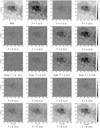 |
Fig. 2 Iterative denoising process for an HMI image with the observation time of July 28, 2020, 20:26:15 under different values of T. The number after L represents the number of iterations. Noise represents denoising starting from Gaussian noise, and the rest starting from the HMI image. |
4.3 Comparative results
Under identical hardware conditions, we trained SAGAN, ICD-DPM, and SDGAN and conducted SR reconstruction on 100 HMI images from the test set. The SR reconstruction times for SAGAN, ICDDPM, and SDGAN were 79 s, 227 s, and 40 s, respectively. The testing times for each HMI image across the three models are illustrated in Fig. 4. The extended reconstruction time for the initial test image can be attributed to the loading of model parameters. It can be observed from Fig. 4 that the reconstruction time of SDGAN and ICDDPM remains relatively stable for each image, whereas the reconstruction time of SAGAN exhibits significant fluctuations. SDGAN demonstrates an advantage in reconstruction efficiency, thereby reducing the computational requirements and resource consumption during sampling. Considering that HMI has accumulated a large amount of observational data and is currently delivering images in a continuous data stream, the enhanced reconstruction speed achieved by SDGAN is beneficial to efficient HMI image research.
The reconstruction results of five HMI images are depicted in Fig. 5. The first three rows exhibit images of active regions containing sunspots and penumbral filaments, and the last two rows depict images of inactive solar areas primarily characterized by solar granules. Subjectively, the reconstructed images from SAGAN, ICDDPM, and SDGAN effectively capture detailed information while preserving the contours, or edges, of the HMI images. Additionally, the spatial resolution of the reconstructed HMI images has been enhanced. SAGAN is capable of reconstructing partial fine structures. However, there are some texture inconsistencies between the reconstructed image and the GST image. One notable difference is observed in the texture direction of the penumbral filaments. ICDDPM excels in reconstructing wider borders of granules and penumbral filaments (Song et al. 2022). However, it is less effective in accurately reproducing the edge textures of granules and sunspots. ICDDPM requires additional adjustments to the brightness of HMI images before sampling, with the aim being to bring the reconstructed images closer to the brightness of GST images. In contrast, SDGAN produces reconstructed images that exhibit greater consistency with GST images, not only in terms of brightness but also in contrast. Additionally, the boundaries of granules and sunspots in the reconstructed images are more pronounced, and the texture direction of penumbral filaments closely resembles that of the GST images.
Figure 6 displays the reconstruction results for small-scale structures in HMI images – such as penumbral filaments, umbral dots, and granules – using SAGAN, ICDDPM, and SDGAN. Notably, SDGAN excels in reconstructing finer structures, yielding clearer results with more natural and detailed structures, indicating that we have achieved our reconstruction objectives.
To further validate the model’s effectiveness in reconstructing HMI images, we processed a total of 833 images captured in a continuous observation sequence from September 1 to 9, 2017. These images were subsequently reconstructed using the models. The reconstructed results were compiled into an animation, as illustrated in Fig. 7. The duration of the animation is 34 s. The reconstructed images in the animation show the typical dynamics of sunspots. From a subjective visual perspective, SAGAN, ICDDPM, and SDGAN all successfully reconstruct numerous image details. It is evident that the reconstruction results of SDGAN are superior in some respects. Notably, there are no artifacts in the reconstructed images produced by SDGAN, and it excels in restoring a greater amount of image detail. This is especially evident in the edge structure of granules, the internal texture of sunspots, and the natural appearance of penumbra filaments.
To quantitatively evaluate the results, we reconstructed 100 test images and calculated four evaluation metrics. Table 2 presents the average results of RMSE, peak S/N, SSIM, and LPIPS between the reconstructed images and GST images. As depicted in Table 2, the results of all three models exhibit improvements across all metrics when compared to HMI images. SDGAN achieves the best average metrics, with RMSE, peak S/N, SSIM, and LPIPS values of 24.7001, 0.5741, 15.4362, and 0.1862, respectively. Figure 8 illustrates a comparison of the evaluation metrics for each reconstructed image generated by SAGAN, ICDDPM, and SDGAN. Overall, the performance indicators of the reconstructed images from all three models show improvement. Compared to the HMI images, the similarity of SDGAN reconstructed images to GST images has significantly improved in terms of pixel fidelity, structural integrity, and perceptual quality. Moreover, the metrics for images reconstructed with SDGAN show that it consistently outperforms SAGAN and ICDDPM, indicating a clear advantage in the quality of SR reconstruction achieved by SDGAN.
The azimuthally averaged power spectrum curves of HMI and GST images, as well as those of the reconstructed images from SAGAN, ICDDPM, and SDGAN, are plotted in Fig. 5 for a comparative analysis of frequency information (see Fig. 9a). The mid-frequency part of the HMI image is low, indicating that there are fewer details in the image. From Fig. 9a, it can be observed that the main difference between the HMI image and the GST image lies in the range of 10–90 Hz, with a peak at 35 Hz. After SR reconstruction, the mid-frequency has been enhanced, and the deviation between the reconstructed image and the GST image is relatively small, indicating that models have achieved some effectiveness in improving image quality and enhancing image details. The curve of the reconstructed SAGAN image closely resembles that of the GST image, but notable fluctuations are observed near the 90Hz frequency. These fluctuations may be attributed to the presence of artifacts or noise in the reconstructed SAGAN image. The curve of the reconstructed image in ICDDPM aligns well with the low-frequency part of the GST image. However, a significant disparity is observed in the high-frequency region. In contrast, the curve of the reconstructed image in SDGAN exhibits greater stability, and compared to ICDDPM, it closely resembles the curve of the GST image. To a certain extent, SDGAN has enhanced the mid-frequency to high-frequency components of the HMI image, resulting in improved preservation of image details.
The HMI image, GST image, and reconstructed image are all grayscale images, and we use the grayscale histogram to evaluate the differences in pixel values among them (see Fig. 9b). The curve of the reconstructed image from SDGAN is more consistent with that of the GST image, indicating that smaller pixel distribution difference. This finding is in line with the RMSE and peak S/N metrics. The pixel values of the reconstructed image from ICDDPM are concentrated around 100, indicating an overall darker image. To further compare the reconstruction results, we used scatter plots to assess the correlation of pixels at corresponding points between GST images and other images (see Figs. 9c–f). Each scatter plot contains 256 × 256 = 65536 data points, and each data point represents a pair of values at corresponding positions in the two images. The proximity of points from other images to those of GST images along a line with a slope of 1 indicates higher pixel similarity. In Fig. 9f, the densely clustered red points near the line with a slope of 1 suggest a smaller pixel difference between the reconstructed image of SDGAN and the GST image.
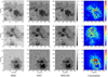 |
Fig. 3 Visualization of SR reconstruction results and the corresponding uncertainty. From left to right are the HMI image, the GST image, the reconstructed image of SDGAN and the corresponding uncertainty estimation. |
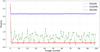 |
Fig. 4 Line chart of the reconstruction time achieved by SAGAN, ICDDPM, and SDGAN for each test image. |
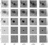 |
Fig. 5 Partial display of SR reconstruction results for images from the test set. Each row from left to right shows an HMI image, a GST image, and an SR reconstructed image from SAGAN, ICDDPM, and SDGAN. |
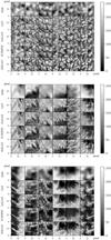 |
Fig. 6 Presentation of reconstruction results for small-scale structures. Top: reconstruction results of solar penumbral filaments. Middle: reconstruction results of solar umbra. Bottom: reconstruction results of solar granules. The HMI in the figure has undergone 4× upsampling. The first row in each image is the HMI image, the second row is the GST image, and the third to fifth rows are the reconstruction results of SAGAN, ICDDPM, and SDGAN for the small-scale structures of HMI images. |
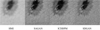 |
Fig. 7 One frame from the animation of SR reconstruction results of HMI images from September 1 to 9, 2017. From left to right, we show the HMI image and reconstructed images of SAGAN, ICDDPM, and SDGAN. The animation is 15 frames s−1 and runs for 34 s; its reconstructed image shows a better representation of the typical dynamics of a sunspot (an animated version of this figure is available online). |
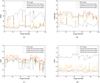 |
Fig. 8 RMSE, peak S/N, SSIM, and LPIPS metrics for SR reconstruction results of images from the test set. The gray, green, orange, and red lines in (a), (b), (c), and (d) represent the metrics calculated by GST images with the corresponding HMI images, images reconstructed by SAGAN, images reconstructed by ICDDPM, and images reconstructed by SDGAN, respectively. |
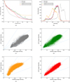 |
Fig. 9 Display of azimuthally average power spectrum plot (panel a), grayscale histogram (panel b) and scatter plots of reconstructed images (panels c, d, e, f). The azimuthally averaged power spectrum plot shows the frequency information of the image, and the grayscale histogram illustrates the density of the pixel distribution. Scatter plots depict the relationship between images. |
Average values of RMSE, peak S/N, SSIM, and LPIPS of the testing results.
5 Conclusion and future work
In this paper, we propose SDGAN, a novel method designed to enhance the spatial resolution of HMI images. SDGAN integrates GANs and DDPM, employing conditional GANs to model the denoising distribution for large-step denoising. Our training data set comprises GST images and HMI images, with the GST image serving as a reference for reconstructing the HMI image at four times the original spatial resolution. Our experimental results demonstrate that SDGAN achieves efficient sampling, producing high-quality reconstructed images. Specifically, SDGAN accomplishes a fourfold spatial resolution reconstruction of HMI images, underscoring its effectiveness. When compared to SAGAN and ICDDPM, SDGAN outperforms in both objective metrics and visual quality, establishing its superiority.
In the future, we plan to explore several different aspects. For model improvement, we aim to investigate more effective ways of integrating GANs and DDPM to further elevate the quality of image reconstruction. Concerning speed optimization, our strategy involves enhancing reconstruction efficiency through techniques such as distillation, pruning, and other methods. Regarding the data set, we are committed to expanding our data set with additional solar images, employing superior image-pairing methods. Furthermore, we intend to curate a comprehensive solar magnetogram data set and leverage SDGAN to enhance the spatial resolution of the solar magnetogram. We hope that this research will provide novel insights into the SR domain of solar images and provide HMI images with higher spatial resolution for solar physics research, allowing more detailed studies of the physical mechanisms of the Sun.
Movies
Movie 1 associated with Fig. 7 Access here
Acknowledgements
The work is supported by the Graduate Research and Practice Projects of Minzu University of China (Grant No: SZKY2023087), the open project of CAS Key Laboratory of Solar Activity (Grant No. KLSA202114), Young Academic Team Leadership Program (Grant No. 2022QNYL31), Ability Enhancement Project for Scientific Research Management (Grant No. 2021GLTS15).
References
- Alshehhi, R. 2022, in 21st International Conference on Image Analysis and Processing (Springer), 451 [Google Scholar]
- Bashir, S. M. A., Wang, Y., Khan, M., & Niu, Y. 2021, PeerJ Comput Sci., 7, e621 [CrossRef] [Google Scholar]
- Baso, C. D., & Ramos, A. A. 2018, A&A, 614, A5 [NASA ADS] [CrossRef] [EDP Sciences] [Google Scholar]
- Deng, J., Song, W., Liu, D., et al. 2021, ApJ, 923, 76 [CrossRef] [Google Scholar]
- Dhariwal, P., & Nichol, A. 2021, Adv. Neural Inform. Process. Syst., 34, 8780 [Google Scholar]
- Dong, C., Loy, C. C., He, K., & Tang, X. 2015, IEEE Trans. Pattern Anal. Mach. Intell., 38, 295 [Google Scholar]
- Gal, Y., & Ghahramani, Z. 2016, in Proceedings of the 33rd International Conference on Machine Learning, 1050 [Google Scholar]
- Gitiaux, X., Maloney, S. A., Jungbluth, A., et al. 2019, arXiv e-print [arXiv:1911.01486] [Google Scholar]
- Goode, P. R., & Cao, W. 2012, Ground-based and Airborne Telescopes IV, Proc. SPIE, 8444, 844403 [NASA ADS] [CrossRef] [Google Scholar]
- Goodfellow, I., Pouget-Abadie, J., Mirza, M., et al. 2020, Commun. ACM, 63, 139 [CrossRef] [Google Scholar]
- He, K., Zhang, X., Ren, S., & Sun, J. 2016, in Proceedings of the IEEE/CVF Conference on Computer Vision and Pattern Recognition, 770 [Google Scholar]
- Ho, J., Jain, A., & Abbeel, P. 2020, in Advances in Neural Information Processing Systems, 6840 [Google Scholar]
- Ho, J., Saharia, C., Chan, W., et al. 2022, JMLR, 23, 1 [Google Scholar]
- Huang, C.-W., Lim, J. H., & Courville, A. C. 2021, Adv. Neural Inform. Process. Syst., 34, 22863 [Google Scholar]
- Isola, P., Zhu, J.-Y., Zhou, T., & Efros, A. A. 2017, in Proceedings of the IEEE/CVF Conference on Computer Vision and Pattern Recognition, 1125 [Google Scholar]
- Jia, P., Huang, Y., Cai, B., & Cai, D. 2019, ApJ, 881, L30 [NASA ADS] [CrossRef] [Google Scholar]
- Karras, T., Laine, S., & Aila, T. 2021, IEEE Trans. Pattern Anal. Mach. Intell., 43, 4217 [CrossRef] [Google Scholar]
- Kingma, D. P., & Ba, J. 2014, arXiv e-print [arXiv:1412.6980] [Google Scholar]
- Ledig, C., Theis, L., Huszár, F., et al. 2017, in Proceedings of the IEEE/CVF Conference on Computer Vision and Pattern Recognition, 4681 [Google Scholar]
- Loshchilov, I., & Hutter, F. 2016, in Proceedings of the International Conference on Learning Representations, 1 [Google Scholar]
- Lowe, D. G. 2004, IJCV, 60, 91 [CrossRef] [Google Scholar]
- Lyu, S. 2009, in Proceedings of the Conference on Uncertainty in Artificial Intelligence, 359 [Google Scholar]
- Mescheder, L., Geiger, A., & Nowozin, S. 2018, in Proceedings of the 35rd International Conference on Machine Learning, PMLR, 3481 [Google Scholar]
- Mirza, M., & Osindero, S. 2014, arXiv e-print [arXiv:1411.1784] [Google Scholar]
- Nelson, C., Doyle, J., Erdélyi, R., et al. 2013, Sol. Phys., 283, 307 [NASA ADS] [CrossRef] [Google Scholar]
- Nichol, A. Q., & Dhariwal, P. 2021, in Proceedings of the 38rd International Conference on Machine Learning, PMLR, 8162 [Google Scholar]
- Park, S. C., Park, M. K., & Kang, M. G. 2003, IEEE Signal Process. Mag., 20, 21 [CrossRef] [Google Scholar]
- Pesnell, W. D., Thompson, B. J., & Chamberlin, P. C. 2012, Sol. Phys., 275, 3 [Google Scholar]
- Rahman, S., Moon, Y.-J., Park, E., et al. 2020, ApJ, 897, L32 [NASA ADS] [CrossRef] [Google Scholar]
- Ronneberger, O., Fischer, P., & Brox, T. 2015, in Medical Image Computing and Computer-Assisted Intervention (Springer), 234 [Google Scholar]
- Saxena, D., & Cao, J. 2021, ACM Comput. Surv., 54, 1 [Google Scholar]
- Scherrer, P. H., Schou, J., Bush, R., et al. 2012, Sol. Phys., 275, 207 [Google Scholar]
- Schwenn, R. 2006, Living Rev. Sol. Phys., 3, 1 [NASA ADS] [CrossRef] [Google Scholar]
- Shumko, S., Gorceix, N., Choi, S., et al. 2014, in Adaptive Optics Systems IV, Proc. SPIE, 1073 [Google Scholar]
- Simonyan, K., & Zisserman, A. 2015, in Proceedings of the International Conference on Learning Representations [Google Scholar]
- Song, Y., Durkan, C., Murray, I., & Ermon, S. 2021a, Adv. Neural Inform. Process. Syst., 34, 1415 [Google Scholar]
- Song, Y., Sohl-Dickstein, J., Kingma, D. P., et al. 2021b, in Proceedings of the International Conference on Learning Representations [Google Scholar]
- Song, W., Ma, W., Ma, Y., Zhao, X., & Lin, G. 2022, ApJS, 263, 25 [NASA ADS] [CrossRef] [Google Scholar]
- Su, Y., Liu, R., Li, S., et al. 2018, ApJ, 855, 77 [NASA ADS] [CrossRef] [Google Scholar]
- Vaswani, A., Shazeer, N., Parmar, N., et al. 2017, Adv. Neural Inform. Process. Syst., 30 [Google Scholar]
- Wang, Z., Bovik, A., Sheikh, H., & Simoncelli, E. 2004, IEEE Trans. Image Process., 13, 600 [CrossRef] [Google Scholar]
- Xiao, Z., Kreis, K., & Vahdat, A. 2021, arXiv e-print [arXiv:2112.07804] [Google Scholar]
- Yang, Q., Chen, Z., Tang, R., Deng, X., & Wang, J. 2023, ApJS, 265, 36 [NASA ADS] [CrossRef] [Google Scholar]
- Zhang, R. 2019, in Proceedings of the 36rd International Conference on Machine Learning, 7324 [Google Scholar]
- Zhang, R., Isola, P., Efros, A. A., Shechtman, E., & Wang, O. 2018, in Proceedings of the IEEE/CVF Conference on Computer Vision and Pattern Recognition, 586 [Google Scholar]
All Tables
All Figures
|
Fig. 1 Architecture of SDGAN. The number after n represents the number of channels in the feature map. Gθ and Dφ are the generator and discriminator modules of SDGAN, respectively. x0 and y represent HR images and LR images, respectively. |
| In the text | |
|
Fig. 2 Iterative denoising process for an HMI image with the observation time of July 28, 2020, 20:26:15 under different values of T. The number after L represents the number of iterations. Noise represents denoising starting from Gaussian noise, and the rest starting from the HMI image. |
| In the text | |
|
Fig. 3 Visualization of SR reconstruction results and the corresponding uncertainty. From left to right are the HMI image, the GST image, the reconstructed image of SDGAN and the corresponding uncertainty estimation. |
| In the text | |
|
Fig. 4 Line chart of the reconstruction time achieved by SAGAN, ICDDPM, and SDGAN for each test image. |
| In the text | |
|
Fig. 5 Partial display of SR reconstruction results for images from the test set. Each row from left to right shows an HMI image, a GST image, and an SR reconstructed image from SAGAN, ICDDPM, and SDGAN. |
| In the text | |
|
Fig. 6 Presentation of reconstruction results for small-scale structures. Top: reconstruction results of solar penumbral filaments. Middle: reconstruction results of solar umbra. Bottom: reconstruction results of solar granules. The HMI in the figure has undergone 4× upsampling. The first row in each image is the HMI image, the second row is the GST image, and the third to fifth rows are the reconstruction results of SAGAN, ICDDPM, and SDGAN for the small-scale structures of HMI images. |
| In the text | |
|
Fig. 7 One frame from the animation of SR reconstruction results of HMI images from September 1 to 9, 2017. From left to right, we show the HMI image and reconstructed images of SAGAN, ICDDPM, and SDGAN. The animation is 15 frames s−1 and runs for 34 s; its reconstructed image shows a better representation of the typical dynamics of a sunspot (an animated version of this figure is available online). |
| In the text | |
|
Fig. 8 RMSE, peak S/N, SSIM, and LPIPS metrics for SR reconstruction results of images from the test set. The gray, green, orange, and red lines in (a), (b), (c), and (d) represent the metrics calculated by GST images with the corresponding HMI images, images reconstructed by SAGAN, images reconstructed by ICDDPM, and images reconstructed by SDGAN, respectively. |
| In the text | |
|
Fig. 9 Display of azimuthally average power spectrum plot (panel a), grayscale histogram (panel b) and scatter plots of reconstructed images (panels c, d, e, f). The azimuthally averaged power spectrum plot shows the frequency information of the image, and the grayscale histogram illustrates the density of the pixel distribution. Scatter plots depict the relationship between images. |
| In the text | |
Current usage metrics show cumulative count of Article Views (full-text article views including HTML views, PDF and ePub downloads, according to the available data) and Abstracts Views on Vision4Press platform.
Data correspond to usage on the plateform after 2015. The current usage metrics is available 48-96 hours after online publication and is updated daily on week days.
Initial download of the metrics may take a while.