| Issue |
A&A
Volume 695, March 2025
|
|
|---|---|---|
| Article Number | A68 | |
| Number of page(s) | 14 | |
| Section | Numerical methods and codes | |
| DOI | https://doi.org/10.1051/0004-6361/202452508 | |
| Published online | 14 March 2025 | |
Composite periodogram analysis for low-event-count fast radio burst repeaters
1
Department of Physics, Faculty of Science, Universiti Malaya,
Kuala Lumpur
50603, Malaysia
2
Institute of Astronomy, National Tsing Hua University,
101, Section 2, Kuang-Fu Road,
Hsinchu
30013, Taiwan
3
Department of Physics, National Chung Hsing University,
145, Xingda Road,
Taichung
40227, Taiwan
★ Corresponding author; taza.aznam@gmail.com
Received:
7
October
2024
Accepted:
30
January
2025
Context. Fast radio bursts (FRBs) are a class of transients characterised by their millisecond-scale duration and relatively high dispersion measures. Some FRBs have been observed to repeat. For such repeating FRBs, measuring the period is key to identifying their physical mechanisms. However, periods have only been measured for two FRBs – FRB 20112002A and FRB 20180916B – because most repeating FRBs have a low event count, making it challenging to measure their periods.
Aims. We aim to introduce a composite periodogram strategy designed to measure periods of repeating FRBs out of low event counts.
Methods. We combined the χ2 periodogram with the inactivity fraction periodogram (F0) to maximise the detection likelihood and minimise noise. Our approach was validated using FRB 20180916B, whereby we successfully recovered the known period with as few as five events. We then applied this method to 17 FRBs whose event counts range from three to 12.
Results. A candidate period is identified in FRB 20190804E, FRB 20190915D, FRB 20200223B, FRB 20201130A, and FRB 20201221B, with a probability of chance coincidence ≤0.050. Additionally, we did further checks to eliminate false positives and concluded that the candidate periods for FRB 20190804E (168.39−0.07+3.86 days) and FRB 20201130A (11.38−0.10+0.10 days) are likely close to its true period. These values provide a basis for informed follow-up observations.
Key words: methods: data analysis / radio continuum: general
© The Authors 2025
 Open Access article, published by EDP Sciences, under the terms of the Creative Commons Attribution License (https://creativecommons.org/licenses/by/4.0), which permits unrestricted use, distribution, and reproduction in any medium, provided the original work is properly cited.
This article is published in open access under the Subscribe to Open model. Subscribe to A&A to support open access publication.
1 Introduction
Fast radio burst (FRB) is a class of transients first discovered by Lorimer et al. (2007) with a currently unknown origin. It is characterised as a radio pulse with durations of the order of milliseconds and a relatively high dispersion measure. Its high dispersion measure suggests an extragalactic origin consistent with observation of identified hosts (Bannister et al. 2019; Chatterjee et al. 2017; Ravi et al. 2019).
Fast radio bursts can be divided into repeaters or one- off FRBs. The population seems to favour one-off FRBs over repeating FRBs. The Canadian Hydrogen Intensity Mapping Experiment/FRB (CHIME/FRB) survey led to a repeater fraction estimate of about  (Andersen et al. 2023). However, a one-off FRB can be re-classified as a repeater FRB if a new signal is associated with the one-off signal. Anticipating this re-classification, Yamasaki et al. (2023) approximated a considerably higher repeater fraction. There is also a lot of research in the FRB literature dedicated to identifying potential repeaters from one-off bursts (Chen et al. 2021; Luo et al. 2022; Zhu-Ge et al. 2023; Pleunis et al. 2021).
Recently, a number of one-off bursts have been re-classified as repeaters with the help of an unsupervised clustering algorithm (Andersen et al. 2023). This discovery serves as the motivation for this paper. Regularly repeating FRBs such as FRB 20121102A, FRB 20180916B, and FRB 20201124A are rare, and newly identified repeaters tend to have low detection counts despite regular daily exposure. With limited data, it is hard to predict when it will happen again, which results in missed opportunities for our further understanding of the origin of FRBs. This study introduces a composite periodogram strategy to address the limited detection count constraint to make a prediction.
2 Repeater periodicity
The periodicity of a repeater can be estimated using a periodogram. A periodogram is a function of metric versus trial period that quantifies the strength of the fit between the given trial period and the time-series data. A trial period with a strong fit will appear as a peak, and the strength relative to neighbouring trial periods will determine the height of such peaks. Table 1 summarises previous methods used to calculate the periodicity of active repeaters using a periodogram.
The Lomb–Scargle periodogram (Lomb 1976; Scargle 1982) is a common astronomical tool for time-series analysis (VanderPlas 2018) that relies on the variation in flux or magnitude. The inactivity fraction method (F0) used by Raj wade et al. (2020) and uniformity measure methods (χ2) used by Amiri et al. (2020); Sand et al. (2023) are useful when information about the light curve and activity cycle is scarce or unknown. Additionally, Li et al. (2024) introduced the phase-folding probability binomial analysis by testing the significance of a central peak at a given trial period.
In this paper, we only use the χ2 and the F0 methods described in Sect. 3. Both methods require the signal function to be folded at the selected trial periods and binned before measuring. These periodograms are known as phase-folding periodograms (VanderPlas 2018). Since they are essentially the same method with different evaluations, we refer to both as metrics and evaluate them in a single pass. In Sect. 4, we continue describing how we used both metrics to evaluate the periodicity of our sample.
Periods of FRBs with different methods in the literature.
3 Periodogram metrics
3.1 Uniformity measure (χ2)
The idea of a uniformity measure for periodicity analysis was introduced in de Jager et al. (1989). Given a time series with an unknown light-curve shape, it is expected to give the maximum difference against a uniform expectation at the phase fold equal to its true periodicity. The authors suggest novel H-test statistics as a uniformity measure, but using Pearson’s chi-squared statistics, χ2, is more common.
Given a telescope’s exposure time, E, towards the designated sky patch in phase bin, ϕ, the χ2 statistics of the period fold is
 (1)
(1)
where Φ is the total number of phase bins, Nϕ is the total number of observed bursts in the ϕ-th bin, and r is the average burst rate of the repeater given by
 (2)
(2)
where N is the number of events and E is the exposure time towards the repeater’s location. We expect different events to accumulate at the same phase bins and cluster around a central peak phase if the signal is folded at its true period. The χ2 periodogram is usually presented in its normalised form by dividing it by the degrees of freedom minus one. We also present it in its normalised form with the more explicit expression χ2/(Φ − 1).
3.2 Inactivity fraction (F0)
This method was described in Rajwade et al. (2020) to tentatively evaluate the periodicity of FRB 20121102A. They measured the longest contiguous inactivity fraction. A long inactive period suggests that the repeater activities are clustered within a certain fraction of each cycle as expected from burst phenomena (Li et al. 2024). The metric can be summarised as the complement of the shortest 1D convex hull containing all events, 1 – min(convex(ϕ)), which we expand to
 (3)
(3)
where ϕ{first/last} is the phase bin number that contains the first or the last event shifted by i-th bin, Φ is the number of bins, and mini(x) is the minimum value of x among all i-th bin shifts. This algorithm can be optimised by knowing that a continued empty- phase bin shift results in the same mini(x) value reducing the total required i shifts from Φ to the number of continuous empty bins. For example, in Fig. 1, there are only two continuous empty bins, so only two shifts give unique values.
Shifting the phase fold to the i-th bin (with the origin rolled over to the end) to find the global minimum is necessary because this metric should be independent of the choice of phase origin. We show this independence in Fig. 1, where the global minimum active region is found with the same value when we account for uncertainty from bin width choices, regardless of the phase origin. We note that the range of this metric is  , and therefore it is an integer multiple of the bin width.
4 Methodology
4.1 Composite periodogram
To overcome the limitation of low event counts of the repeaters, we propose using a biperiodogram scheme so that mutual peaks will correlate but noisy peaks will be muted by the partnering metric. We combined χ2 and F0 metrics to create a χ2−F0 composite periodogram. Each trial period will be assigned a probability of chance coincidence, Pcc, based on the trial periods’ χ2−F0 pair. The probability model is generated from a simulation described in Sect. 4.5. Since F0 measures variation in the phase space and χ2 measures variation in the magnitude space of a given phase fold, the χ2−F0 composite is analogous to studying the activity variation versus the activity concentration.
4.2 Signal function
The signals of FRB repeater events are treated as pure delta functions with a magnitude of 1 at the time of arrivals (TOAs) and 0 everywhere else:
 (4)
(4)
This formulation ignores fluence and energy variations between events but allows us to measure the periodic modulation of the repeaters. The periods for both FRB 20111202A (Rajwade et al. 2020; Cruces et al. 2021; Li et al. 2024) and FRB 20180916B (Amiri et al. 2020; Sand et al. 2023) are measured in terms of periodically modulated activity because bursty phenomena tend to show increasing burst rates in the active phase (Li et al. 2024). The metrics chosen for this study are optimised for finding this concentration of event along the phases. TOA data are obtained from the CHIME/FRB Public Database web site1. These TOAs are topocentric, so we used ‘astropy’2 to convert them to barycentric TOAs before evaluating them.
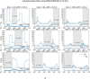 |
Fig. 1 Example phase-folds using FRB 20180916B at 32.56 days with different bin numbers and phase-origin shifts. For each sub-figure, the top figure is the histogram of observed bursts (solid blue) and uniform expectation (dashed green) in each phase bin with the residue displayed in the bottom figure. The χ2 metric is proportional to the sum of the squared value of this residue. The grey span in the histogram shows the inactivity fraction (F0). |
4.3 Exposure function and observation window
The CHIME telescope is a transit telescope oriented in the N- S direction that operates 24 hours daily in nominal conditions. Therefore, the exposure function depends on the Earth’s rotation and the computational operation. We followed the method of Amiri et al. (2021), which considers the sky to be exposed if it is within the full-width-at-half-maximum (FWHM) region of the synthesised beam at 600 MHz with an operational CPU node.
We utilised the daily exposure data provided by CHIME/FRB between 28 Aug 2018 and 1 May 2021 inclusive3. It is stored at four seconds of resolution as a HealPix array (Górski et al. 2005) under a ring configuration with the ‘nside’ parameter equal to 4096. We extracted the exposure duration (in hours) of the sky position of each sample as a function of day. The uncertainty in exposure is modelled as a purely geometric function of declination because it is constant in right ascension (Amiri et al. 2021; Yamasaki et al. 2023):
 (5)
(5)
We then set the date range of this exposure function as the observation window (T = 977 days) of this paper.
4.4 Trial period fold configuration
We evaluated the trial periods, P, across two ranges: the primary range is between 1.5 < P ≤ τ days while the secondary range is between τ < P ≤ 2τ days, where τ as the time difference between the last and first events (the event window). We find our candidate periods only within the primary range. We used the secondary range to calculate the probability of chance coincidence, Pcc in Sect. 4.5. We consider this secondary range as random noise; thus, including it to calculate Pcc tightens the constraints. The secondary range is also useful for understanding the behaviour of the periodograms at the search boundary, which is clear in Sect. 6.3.
The trial period range is spaced at  day spacing, where r is the average burst rate of the repeater (Eq. (2)). We found that reducing the range spacing (e.g. using 1/(nr), n > 1 spacing) gives the same result as our chosen spacing. Moreover, since our probability model uses the same trial period range, we obtained the same probability models even with a finer spacing. Therefore, reducing the trial period spacing adds computational cost with no added benefit.
We set the phase origin to 28 Aug. 2018 at 00:00:00 h for all trial period folds. We then binned the number of signals with the bin width equal to ten degrees each, making the number of bins Φ = 36. We found this number to balance the granularity of the F0 metric and the sparseness of the events in a low-event-count repeater. This is because increasing the bin width will make F0 less precise, but decreasing the bin width will make fewer events accumulate within the same bin, thereby reducing the activity variation per phase. As seen in Fig. 1, increasing the number of bins does not significantly increase the precision of F0, but at the same time it reduces the χ2 metric value because of the reduced event count per phase bin. Figure 1 also shows the effect of shifting the phase origin that only shows minimal differences.
The exposure function is also folded and binned with the same configuration. This serves as the Eϕ value to build the uniform expectation function for our χ2 metric (Eq. (1)). Since the exposure function has a daily precision, we set the exposure to occur at 00:00:00 h every day, affecting the resulting binned curve. At the same time, the TOA values reported in the CHIME/FRB public database are given to subsecond precision levels. This mismatch in precision prevented us from directly comparing the values within a continuous phase domain. By binning the phases, we minimised the effects caused by this difference in precisions.
4.5 Probability of chance coincidence, Pcc
We assign a probability at each trial period based on the probability of each metric pair. It is unlikely for both metrics to peak at the same time in a scenario with random data. We define the probability of chance coincidence, Pcc , for each trial period, P, given that the metric pairs are observed as
 (6)
(6)
where  is the cumulative density function (CDF) value for the χ2−F0 pair generated from the simulation’s
  pair. The subscript ‘sim’ highlights the role of the simulation as a tool to generate the CDF. We aim to find the trial period where Pcc is minimised. The uncertainty is taken as the width of the peak where Pcc(P |χ2, F0) = 0.050.
The CDF in Eq. (6) is generated by simulating 100 scenarios of events randomly occurring within the same observation window. We used the burst rate of each repeater to encode their property into the model. The steps are described below:
Determine the burst rate, r, of the repeater using Eq. (2).
For each simulation:
- (a)
Generate a series of TOAs between 28 August 2018 and 1 May 2021 inclusive, where the event probability at time t is the product of r and exposure E(t):
 (7)
(7)This should give a roughly equal amount of event counts distributed randomly across the observation window.
- (b)
Evaluate both metrics.
- (c)
Accumulate the metrics into their respective collection. The order of the collection should be preserved.
Generate a bivariate normal distribution with the same mean and covariance values as the metric pairs. This bivariate normal distribution is the CDF of the sample. It means the probability that any value X and Y is lower than or equal to the current value x and y:
 (8)
(8)
- (a)
5 Testing our method using FRB 20180916B
5.1 Full observation window
To test the validity of our method, we evaluated the period of FRB 20180916B. We chose this FRB for our test because it is part of the CHIME/FRB catalogue, it has events within the observation window, and it has a measured periodicity (Amiri et al. 2020; Sand et al. 2023). From Fig. 2, we find that our method evaluated the period of  days – which is well within the previously measured periodicity ranges (see Table 1).
5.2 Limiting the observation window
Our second test involves limiting the current observation window of FRB 20180916B into shorter and shorter time frames. By artificially limiting the observation window, we mimic the properties of our repeater sample, which features repeaters with low event counts. By doing so, we demonstrate two properties of our method: (i) the evaluated period is independent of the number of event counts, and (ii) this method can find the periodicity even at low event counts.
For this test, we cut the T = 977 days observation window, into 98-day interval increments, which equates to roughly 10% of the original observation window. This interval increment creates ten subsets for FRB 20180916B. Each subset is selected as FRB 20180916B events that occur within {98,196,294,392,490,588,686,784, 882,977} days of the start of the original observation window (28 Aug 2018). We note that there is a discrepancy in the final interval jump; that is, a 95- day increment – as opposed to a 98-day increment – which is inconsequential to our interest in the low-event-count analysis. For simplicity, we refer to these subsets by the percentages of the original observation window; for example, 10% T.
We can see from Fig. 3 that the evaluated periods are consistent with previous results regardless of the number of events. One notable deviation is the result from the 10% observation window with five event counts, but it still has uncertainty within the established period. Other than that, we can see a general trend of increasing uncertainty as we go down the event counts.
5.3 Alternative view: Metric-metric plot
We plot the values of one metric, F0 , against another metric, χ2 , ignoring the trial period values. This creates a 2D analogue of the two 1D periodogram plots. By using this metric-metric plot, we can see how the number of event counts affects the distribution of the metrics. This view also allows us to compare the distribution of the metrics across the repeater sample done in Sect. 6.
The general distribution of the metric-metric plot is clustered around a mean and smeared towards either χ2 or F0. However, the plots consistently feature a primary tail (red diamond) pointing towards the +χ2, + F0 direction. The end of the primary tail is longer with higher event counts, indicating a higher correlation and confidence. These tails are metric pairs with Pcc ≤ 0.050. In an ideal case where points with lower Pcc consistently correlate, it resembles a tail, as can be seen in the 40% T and 30% T sub-plots for Fig. 4. Even with no prominent primary tail at a 10% observation window, the metric-metric plot still managed to find a significant peak over the Pcc ≤ 0.050 threshold.
Another feature that is noticeable in the metric-metric plot is how the secondary period range (orange cross and green square) evolves as the observation window changes. In small observation windows, the metric pairs of the secondary period range distribute closely to the primary period range, but as the observation window becomes larger, it distributes independently, smearing towards the + F0 direction. This highlights the different sensitivities of the different metrics. This secondary period range bias is suppressed by the χ2, which is less sensitive to this bias (and vice versa), allowing for the correlation tail to emerge and thus identifying the true peak.
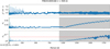 |
Fig. 2 Individual periodograms for χ2 and F0 metric stacked on top of each other and Pcc for FRB 20180916B at full observation window. The y-axis of Pcc is inverted to match the peak pattern of both metrics. The red dash-dotted line shows the Pcc ≤ 0.050 threshold. The green line and span show the evaluated period and its error. The grey span shows the secondary trial period range. |
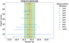 |
Fig. 3 Event count plotted against evaluated periods for FRB 20180916B with limited observation window. The 100% window is coloured red to highlight the result from a full dataset. The green vertical hatch and the orange diagonal hatch represent period ranges from Amiri et al. (2020) and Sand et al. (2023), respectively. |
6 Result: Candidate periods
6.1 Data selection
The sample for this paper is taken from the ‘golden’ sample repeaters identified in Andersen et al. (2023). The original ‘golden’ sample lists 25 repeaters, but we only select repeaters with three or more events within the observation window. The candidates are now reduced to 17 repeaters ranging from three to 12 events for each repeater; these are listed in Table 2.
6.2 Composite periodogram
Applying the composite periodogram method to our selected samples, we find that the shape of these metric–metric plots (Fig. 5) generally follows the shape of FRB 20180916B’s plot (Fig. 4) when the observation window is limited below 50%; this represents a smeared cluster with no prominent primary tail including a secondary period range with similar distribution as primary period range. We found five repeaters with trial periods crossing the Pcc ≤ 0.050 threshold. The trial periods with the lowest Pcc for all repeaters are tabulated in Table 2.
6.3 Anomaly check
In this section, we compare the properties of the five repeaters with a candidate period with some additional properties from FRB 20180916B to check for anomalies. For this check, we introduced two properties: (i) the average number of days between events relative to the period, D, and (ii) the relative difference of the period from the event window. The average number of days between events relative to the period, D, is calculated using the equation
 (9)
(9)
where τ is the event window, n is the event count, and P is the evaluated period, in days.
The first check ensures that the repeaters show activity clustering. The second check ensures that the evaluated period is free from aliasing. Aliasing can occur when the trial period is equal to the event window, causing the first and last events to overlap in the same phase bin. With a low event count, this overlap skews the F0 metric towards higher values. Appendix B discusses this aliasing further.
Figure 6 shows that the period of FRB 20180916B closely matches the average days between events, D, with values of D ≲ 1 showing signs of activity clustering. By comparing this property with our sample, among the five repeaters with Pcc ≤ 0.050, we find three anomalous repeaters whose values are far away from the D = 1 line in either direction.
We first dismiss the FRBs with D ≫ 1, which are FRB 20190915D and FRB 20200223B, because our test sample, FRB 20180916B, does not have D ≫ 1. This sparseness indicates that at least one event is detected every 3.23 cycles (FRB 20190915D) or 3.27 cycles (FRB 20200223B) which does not make sense. It is certainly doubtful whether they truly repeat at these evaluated periods. This anomaly might be caused by one of three things: (i) some or most of the events for these repeaters being missed, especially due to CHIME being rarely exposed to low declinations Amiri et al. (2021) for FRB 20200223B; (ii) the true period being D times the evaluated period; or (iii) the evaluated period being false.
Possibility (i) might be related to possibility (ii), but it does not necessitate the latter. It simply means that the probability of coincidence is lower when there are false non-detections. Possibility (ii) can be illustrated with the analysis done by Voisin et al. (2021), where they argue that the orbital period is three times the evaluated period for FRB 20180916B in their asteroid- assisted emission model. However, FRB 20180916B is already shown to have D ≲ 1, so the suggested emission model should give a result as if the evaluated period is the true period, making this possibility unlikely.
Now we discuss FRB 20201221B with D = 0.2, making it the lowest out of all samples. Although D < 1 shows signs of activity clustering, FRB 20180916B has D value within a reasonable difference compared to its period (0.8 ≲ D ≲ 1.0). When comparing with its closeness to the event window, τ (Fig. 7), it is evident that the evaluated period for FRB 20201221B is near the search boundary. A glance at the generated periodogram in Fig. C.6 reveals it is a plateau from aliasing in F0 near the P ~ τ region and not a peak. In retrospect, the metric-metric plot (Fig. 5) shows that the primary tail and secondary tail for FRB 20201221B are indistinguishable, which is not the case for FRB 20180916B and the other repeaters.
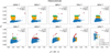 |
Fig. 4 Metric-metric plot for different observation windows (T=977 days) of FRB 20180916B. The blue plus sign and red diamonds represent the primary period range, while the orange cross and the green square represent the secondary period range. The red diamond (primary tail) and the green square (secondary tail) represent trial periods that cross the Pcc ≤ 0.050 threshold for their respective period ranges. The point circled in black denotes the lowest Pcc. |
Properties of FRB sample with its evaluated values.
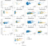 |
Fig. 5 Metric-metric plot for sample of 17 repeaters. The colours have the same meaning as in Fig. 4. The grid-like structure found along the F0 direction occurs because it is an integer multiple of the phase-bin width (see Sect. 3.2). Some repeaters show no primary tail, but we still circle the Pcc with the lowest value. |
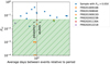 |
Fig. 6 Probability of chance coincidence plotted against the average days between events for our sample with values from FRB 20180916B as reference. The various plot points for FRB 20180916B represent the values from different sub-windows. Points at the bottom line indicate probability values lower than the graph limit. |
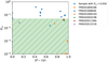 |
Fig. 7 Probability of chance coincidence plotted against relative difference of period from event window for our sample with values from FRB 20180916B as reference. The various plot points for FRB 20180916B represent the values from different sub-windows. Points at the bottom line indicate probability values lower than the graph limit. |
6.4 Acceptance criteria
Using the quick anomaly check described in the previous section, we find two criteria to accept a trial period, P, from a composite periodogram:
The average number of days between events must be reasonably close to the evaluated period. This paper does not attempt to provide a hard limit of how close the value should be, so this is done purely from visual inspection.
The chosen trial period must be distinguishable from the secondary tail of the metric–metric plot. Being indistinguishable is a sign that it is not a peak but a plateau near the search boundary (P ~ τ) spanning both P ≤ τ and P > τ.
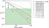 |
Fig. 8 Probability of chance coincidence of evaluated period plotted against the event counts of the FRB. Points along the bottom line of the y-axis show values below the graph limit. |
7 Constraining event counts
With a newly identified repeater, one may wonder how many detections are necessary to be able to evaluate its periodicity. Since active repeaters are rare, considering this question helps shape future observations for non-active repeaters. Figure 8 shows how the probability of coincidence of the evaluated periods is distributed across different event counts.
By visual inspection, we found that the maximum Pcc obtainable at each event count follows a power law, thus creating an upper limit. To find this upper limit, we first define the power law as always less than one:
 (10)
(10)
The value of α and k can be found by first setting αn−k = 1 and algebraically rearranging it to be
 (11)
(11)
By setting n = 2, we define the Pcc upper limit because that is the minimum valid integer required to satisfy k ≠ 0. We find that α = 3 with k = 1.58 rests neatly on the points that make up the upper limit border.
This upper limit implies that at n = 40 we can be certain that this method can find the period of the FRB with a high enough confidence level (Pcc ≤ 0.050) assuming the FRB has a true periodicity. For n < 40, we found that at n = 4 the maximum Pcc is 0.500, allowing us to adjust our expectations accordingly.
8 Summary
This paper proposes the use of a composite periodogram to evaluate the candidate period of FRBs with low event counts to facilitate follow-up observations. The composite periodogram presented in this paper is a combination of a uniformity measure periodogram (χ2) and an inactivity fraction periodogram (F0). We also present some checks for anomalies to reject false positives. Our analysis shows the following:
Fast radio bursts with true period values show a primary tail in the metric–metric plot distinguishable from the secondary tail. The length of the primary tail of the metric-metric plot has an inverse relationship with the evaluated period uncertainty. A shorter primary tail corresponds to high uncertainty, while a longer primary tail corresponds to low uncertainty. Primary tails that are indistinguishable from the secondary tails should be further inspected. The candidate period of FRB 20201221B is rejected following this inspection.
Using the result from FRB 20180916B as a criterion, we found that the average number of days between events, D, should roughly correspond to the period obtained. The candidate periods for FRB 20190915D and FRB 20200223B are rejected because of their D ≫ 1.
Using the composite period to evaluate a candidate period, and doing the checks described in items 1 and 2, we tentatively identify the candidate periods of FRB 20190804E (
 days) and FRB 20201130A (
 days). We encourage the scheduling of follow-up observations after this assumed period.
Acknowledgements
The authors wish to thank the team from CHIME/FRB for providing open data which allowed this work to happen and Ziggy Pleunis whose discussion with MA in the “Localization of fast radio bursts in Taiwan 2024” conference (June 2024) improved the result of this study. TH acknowledges the support of the National Science and Technology Council of Taiwan through grants 113-2112-M-005-009-MY3 and 113-2123-M-001-008-. TG acknowledges the support of the National Science and Technology Council of Taiwan through grants 113-2112-M-007-006-, 113-2927I-007-501-, and 113-2123-M-001-008-.
Appendix A Resulting phase-folded data
In this section we show the results of folding the data at the evaluated period for our sample in Fig. A.1 to give a more complete picture of our result. The residue, Nϕ − r⋅Eϕ, is not shown in this figure because the uniform expectation functions are too uniform compared to available data making the resulting residue resemble the original distribution. We can see that the data is tightly distributed around a central peak except for FRB 20191139A having two prominent peaks.
These shapes are expected for data that is folded at the correct period. However, the challenge arises in low-event-count FRB repeaters because lower event counts gives a limited number of distribution. That is to say that we can distribute 3 events randomly in several ways as opposed to distributing 30 random events in many different ways. This limited number of configurations means a tight distribution around a central peak is just as likely as any highly distributed data for a low data count. Running a random aperiodic simulation in Sect. 4.5 mitigates this effect by encoding the information of the number of events and the burst rate into the probability.
Appendix B Individual periodograms
In this paper, we introduced a metric–metric plot (see Sect. 5.3) to show the overall effects of the combination of periodogram metrics across the whole sample. In this section we present the individual metrics as a function of trial periods stacked on top of each other and Pcc for selected FRBs to highlight the effect in individual samples. We show the plots for FRB 20180916B (at 10% T), FRB 20190804E, FRB 20190915D, FRB 20200223B, FRB 20201130A, and FRB 20201221B.
The colours in the figures have the same meaning as Fig. 2 but we rewrite it here for simplicity. The red dash-dotted line shows the Pcc ≤ 0.050 threshold. The green line and span show the evaluated period and its error. The grey span shows the secondary trial period range. The y-axis of Pcc is inverted to match the peak pattern of both metrics. Thus, in this section we refer to points with low Pcc as peaks to follow the visual.
We see that both metrics’ peaks amplify each other resulting in a strong peak in Pcc . The inverse is true in periods where a peak is observed in only one metric and not the other, resulting in a suppression of peaks in Pcc . In this way, a noisy periodogram in any of the χ2 or F0 metric becomes less noisy in Pcc.
The F0 periodogram shows a tendency to plateau near the event window. This plateau occurs because when the trial period is equal to the event window, the first and the last events overlap at the same phase bin, giving the illusion that the FRB concentrates its activity at that period fold. At high event counts, this illusion is not apparent because of how all the other events are distributed across the phase bins. This illusion is only significant in low event counts resulting in higher F0 values.
Due to the property of the composite periodogram discussed previously, the plateau can be made insignificant with a strong enough suppression from the χ2 periodogram. However, it also means that the F0 plateau can directly impact the Pcc result if the suppression is weak. Some different cases of this plateau are seen:
A plateau near τ but the plateau is not higher than its chosen period peak (FRB 20180916B and FRB 20190804E).
A plateau near or just before τ with almost the same height as its chosen period (FRB 20190915D and FRB 20200223B).
A plateau after τ with almost the same height as its chosen period (FRB 20201130A).
A plateau at τ with no other contesting peak (FRB 20201221B).
These different cases for the F0 plateau correspond neatly with our selection criteria purely based on the composite periodogram and anomaly checks. FRB 20190804E have an insignificant plateau and FRB 20201130A have a plateau after τ with an accepted trial period. Since the secondary trial period range, τ < P ≤ 2τ, is not considered for the period, this case of plateau does not impact the result. FRB 20190915D and FRB 20200223B have a F0 plateau with almost the same height as other peaks, which shows an anomaly of D ≫ 1 and is thus rejected. FRB 20201221B has a F0 plateau near τ with no competing peaks, which shows a D ~ 0 anomaly and is also rejected.
Appendix C A combined statistic?
It is possible to create a new combined statistic such as
 (C.1)
(C.1)
where a is a ratio that quantifies the contribution of each metric. However, using this approach, after determining the parameters of this new statistic using FRB 20180916B, we would need to establish that the parameters are independent of sample choice, whose burst rate varies. It would be a circular task to determine the period and the universality of the parameters using the same sample. The method that we proposed in this paper takes into account the differences in sample properties by encoding the burst rate into the probability model.
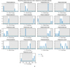 |
Fig. A.1 Phase-folded data for our sample of 17 repeaters showing the distribution of activities as a function of phase. The data is folded at their respective evaluated periods. The blue solid line shows the event count at the phase bin. The green dashed line shows the uniform expectation function derived from the exposure function and burst rate. The grey span shows the inactive region whose length is F0. FRBs with an asterisk near their name are FRBs with Pcc ≥ 0.050. |
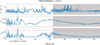 |
Fig. C.1 Individual periodograms for χ2 and F0 metric stacked on top of each other and Pcc for FRB 20180916B at 10% T (T = 977 days). The y-axis of Pcc is inverted to match the peak pattern of both metrics. The text clarifies the meaning of the colours. |
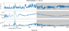 |
Fig. C.2 Individual periodograms for χ2 and F0 metric stacked on top of each other and Pcc for FRB 20190804E. The y-axis of Pcc is inverted to match the peak pattern of both metrics. The text clarifies the meaning of the colours. |
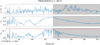 |
Fig. C.3 Individual periodograms for χ2 and F0 metric stacked on top of each other and Pcc for FRB 20190915D. The y-axis of Pcc is inverted to match the peak pattern of both metrics. The text clarifies the meaning of the colours. |
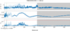 |
Fig. C.4 Individual periodograms for χ2 and F0 metric stacked on top of each other and Pcc for FRB 20200223B. The y-axis of Pcc is inverted to match the peak pattern of both metrics. The text clarifies the meaning of the colours. |
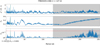 |
Fig. C.5 Individual periodograms for χ2 and F0 metric stacked on top of each other and Pcc for FRB 20201130A. The y-axis of Pcc is inverted to match the peak pattern of both metrics. The text clarifies the meaning of the colours. |
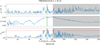 |
Fig. C.6 Individual periodograms for χ2 and F0 metric stacked on top of each other and Pcc for FRB 20201221B. The y-axis of Pcc is inverted to match the peak pattern of both metrics. The text clarifies the meaning of the colours. |
References
- Amiri, M., Andersen, B. C., Bandura, K. M., et al. 2020, Nature, 582, 351 [NASA ADS] [CrossRef] [Google Scholar]
- Amiri, M., Andersen, B. C., Bandura, K., et al. 2021, ApJS, 257, 59 [NASA ADS] [CrossRef] [Google Scholar]
- Andersen, B. C., Bandura, K., Bhardwaj, M., et al. 2023, ApJ, 947, 83 [NASA ADS] [CrossRef] [Google Scholar]
- Bannister, K. W., Deller, A. T., Phillips, C., et al. 2019, Science, 365, 565 [NASA ADS] [CrossRef] [Google Scholar]
- Chatterjee, S., Law, C. J., Wharton, R. S., et al. 2017, Nature, 541, 58 [NASA ADS] [CrossRef] [Google Scholar]
- Chen, B. H., Hashimoto, T., Goto, T., et al. 2021, MNRAS, 509, 1227 [NASA ADS] [CrossRef] [Google Scholar]
- Cruces, M., Spitler, L. G., Scholz, P., et al. 2021, MNRAS, 500, 448 [Google Scholar]
- de Jager, O. C., Raubenheimer, B. C., & Swanepoel, J. W. H. 1989, A&A, 221, 108 [Google Scholar]
- Górski, K. M., Hivon, E., Banday, A. J., et al. 2005, ApJ, 622, 759 [Google Scholar]
- Li, J., Gao, Y., Li, D., & Wu, K. 2024, ApJ, 969, 23 [NASA ADS] [CrossRef] [Google Scholar]
- Lomb, N. R. 1976, Astrophys. Space Sci., 39, 447 [Google Scholar]
- Lorimer, D. R., Bailes, M., McLaughlin, M. A., Narkevic, D. J., & Crawford, F. 2007, Science, 318, 777 [Google Scholar]
- Luo, J.-W., Zhu-Ge, J.-M., & Zhang, B. 2022, MNRAS, 518, 1629 [CrossRef] [Google Scholar]
- Pleunis, Z., Good, D. C., Kaspi, V. M., et al. 2021, ApJ, 923, 1 [NASA ADS] [CrossRef] [Google Scholar]
- Rajwade, K. M., Mickaliger, M. B., Stappers, B. W., et al. 2020, MNRAS, 495, 3551 [NASA ADS] [CrossRef] [Google Scholar]
- Ravi, V., Catha, M., D’Addario, L., et al. 2019, Nature, 572, 352 [NASA ADS] [CrossRef] [Google Scholar]
- Sand, K. R., Breitman, D., Michilli, D., et al. 2023, ApJ, 956, 23 [NASA ADS] [CrossRef] [Google Scholar]
- Scargle, J. D. 1982, ApJ, 263, 835 [Google Scholar]
- VanderPlas, J. T. 2018, ApJS, 236, 16 [Google Scholar]
- Voisin, G., Mottez, F., & Zarka, P. 2021, MNRAS, 508, 2079 [NASA ADS] [CrossRef] [Google Scholar]
- Yamasaki, S., Goto, T., Ling, C.-T., & Hashimoto, T. 2023, MNRAS, 527, 11158 [NASA ADS] [CrossRef] [Google Scholar]
- Zhu-Ge, J.-M., Luo, J.-W., & Zhang, B. 2023, MNRAS, 519, 1823 [Google Scholar]
All Tables
All Figures
|
Fig. 1 Example phase-folds using FRB 20180916B at 32.56 days with different bin numbers and phase-origin shifts. For each sub-figure, the top figure is the histogram of observed bursts (solid blue) and uniform expectation (dashed green) in each phase bin with the residue displayed in the bottom figure. The χ2 metric is proportional to the sum of the squared value of this residue. The grey span in the histogram shows the inactivity fraction (F0). |
| In the text | |
|
Fig. 2 Individual periodograms for χ2 and F0 metric stacked on top of each other and Pcc for FRB 20180916B at full observation window. The y-axis of Pcc is inverted to match the peak pattern of both metrics. The red dash-dotted line shows the Pcc ≤ 0.050 threshold. The green line and span show the evaluated period and its error. The grey span shows the secondary trial period range. |
| In the text | |
|
Fig. 3 Event count plotted against evaluated periods for FRB 20180916B with limited observation window. The 100% window is coloured red to highlight the result from a full dataset. The green vertical hatch and the orange diagonal hatch represent period ranges from Amiri et al. (2020) and Sand et al. (2023), respectively. |
| In the text | |
|
Fig. 4 Metric-metric plot for different observation windows (T=977 days) of FRB 20180916B. The blue plus sign and red diamonds represent the primary period range, while the orange cross and the green square represent the secondary period range. The red diamond (primary tail) and the green square (secondary tail) represent trial periods that cross the Pcc ≤ 0.050 threshold for their respective period ranges. The point circled in black denotes the lowest Pcc. |
| In the text | |
|
Fig. 5 Metric-metric plot for sample of 17 repeaters. The colours have the same meaning as in Fig. 4. The grid-like structure found along the F0 direction occurs because it is an integer multiple of the phase-bin width (see Sect. 3.2). Some repeaters show no primary tail, but we still circle the Pcc with the lowest value. |
| In the text | |
|
Fig. 6 Probability of chance coincidence plotted against the average days between events for our sample with values from FRB 20180916B as reference. The various plot points for FRB 20180916B represent the values from different sub-windows. Points at the bottom line indicate probability values lower than the graph limit. |
| In the text | |
|
Fig. 7 Probability of chance coincidence plotted against relative difference of period from event window for our sample with values from FRB 20180916B as reference. The various plot points for FRB 20180916B represent the values from different sub-windows. Points at the bottom line indicate probability values lower than the graph limit. |
| In the text | |
|
Fig. 8 Probability of chance coincidence of evaluated period plotted against the event counts of the FRB. Points along the bottom line of the y-axis show values below the graph limit. |
| In the text | |
|
Fig. A.1 Phase-folded data for our sample of 17 repeaters showing the distribution of activities as a function of phase. The data is folded at their respective evaluated periods. The blue solid line shows the event count at the phase bin. The green dashed line shows the uniform expectation function derived from the exposure function and burst rate. The grey span shows the inactive region whose length is F0. FRBs with an asterisk near their name are FRBs with Pcc ≥ 0.050. |
| In the text | |
|
Fig. C.1 Individual periodograms for χ2 and F0 metric stacked on top of each other and Pcc for FRB 20180916B at 10% T (T = 977 days). The y-axis of Pcc is inverted to match the peak pattern of both metrics. The text clarifies the meaning of the colours. |
| In the text | |
|
Fig. C.2 Individual periodograms for χ2 and F0 metric stacked on top of each other and Pcc for FRB 20190804E. The y-axis of Pcc is inverted to match the peak pattern of both metrics. The text clarifies the meaning of the colours. |
| In the text | |
|
Fig. C.3 Individual periodograms for χ2 and F0 metric stacked on top of each other and Pcc for FRB 20190915D. The y-axis of Pcc is inverted to match the peak pattern of both metrics. The text clarifies the meaning of the colours. |
| In the text | |
|
Fig. C.4 Individual periodograms for χ2 and F0 metric stacked on top of each other and Pcc for FRB 20200223B. The y-axis of Pcc is inverted to match the peak pattern of both metrics. The text clarifies the meaning of the colours. |
| In the text | |
|
Fig. C.5 Individual periodograms for χ2 and F0 metric stacked on top of each other and Pcc for FRB 20201130A. The y-axis of Pcc is inverted to match the peak pattern of both metrics. The text clarifies the meaning of the colours. |
| In the text | |
|
Fig. C.6 Individual periodograms for χ2 and F0 metric stacked on top of each other and Pcc for FRB 20201221B. The y-axis of Pcc is inverted to match the peak pattern of both metrics. The text clarifies the meaning of the colours. |
| In the text | |
Current usage metrics show cumulative count of Article Views (full-text article views including HTML views, PDF and ePub downloads, according to the available data) and Abstracts Views on Vision4Press platform.
Data correspond to usage on the plateform after 2015. The current usage metrics is available 48-96 hours after online publication and is updated daily on week days.
Initial download of the metrics may take a while.