| Issue |
A&A
Volume 695, March 2025
|
|
|---|---|---|
| Article Number | A40 | |
| Number of page(s) | 12 | |
| Section | The Sun and the Heliosphere | |
| DOI | https://doi.org/10.1051/0004-6361/202452426 | |
| Published online | 03 March 2025 | |
Coronal energy release by MHD avalanches
III. Identification of a reconnection outflow from a nanoflare
1
Dipartimento di Fisica & Chimica, Università di Palermo, Piazza del Parlamento 1, I-90134 Palermo, Italy
2
INAF-Osservatorio Astronomico di Palermo, Piazza del Parlamento 1, I-90134 Palermo, Italy
3
Harvard–Smithsonian Center for Astrophysics, 60 Garden St., Cambridge, MA 02193, USA
4
Lockheed Martin Solar & Astrophysics Laboratory, 3251 Hanover St, Palo Alto, CA 94304, USA
5
Rosseland Centre for Solar Physics, University of Oslo, P.O. Box 1029 Blindern N-0315 Oslo, Norway
6
Institute of Theoretical Astrophysics, University of Oslo, P.O. Box 1029 Blindern N-0315 Oslo, Norway
7
SETI Institute, 339 Bernardo Ave, Suite 200, Mountain View, CA 94043, USA
⋆ Corresponding author; This email address is being protected from spambots. You need JavaScript enabled to view it.
Received:
30
September
2024
Accepted:
2
February
2025
Abstract
Context. Outflows perpendicular to the guide field are believed to be a possible signature of magnetic reconnection in the solar corona. Specifically, outflows can help detect the occurrence of ubiquitous small-angle magnetic reconnection.
Aims. The aim of this work is to identify possible diagnostic techniques of such outflows in hot coronal loops with the Atmospheric Image Assembly (AIA) on board the Solar Dynamics Observatory and the forthcoming MUltislit Solar Explorer (MUSE), in a realistically dynamic coronal loop environment where a magnetohydrodynamic (MHD) avalanche is occurring.
Methods. We considered a 3D MHD model of two magnetic flux tubes, including a stratified, radiative, and thermal-conducting atmosphere, twisted by footpoint rotation. The faster rotating flux tube becomes kink-unstable and soon involves the other one in the avalanche. The turbulent decay of this magnetic structure on a global scale leads to the formation, fragmentation, and dissipation of current sheets, driving impulsive heating akin to a nanoflare storm. We captured a clear outflow from a reconnection episode soon after the initial avalanche and synthesised its emission as detectable with AIA and MUSE.
Results. The outflow has a maximum temperature around 8 MK, total energy of 1024 erg, velocity of a few hundred km/s, and duration of less than 1 min. We show the emission in the AIA 94 Å channel (Fe XVIII line) and in the MUSE 108 Å Fe XIX spectral line.
Conclusions. This outflow shares many features with nanojets recently detected at lower temperatures. However, its low emission measure makes its detection difficult with AIA, while Doppler shifts can be measured with MUSE. Conditions become different in the later steady-state phase, when the flux tubes are filled with denser and relatively cooler plasma.
Key words: magnetic reconnection / magnetohydrodynamics (MHD) / Sun: corona / Sun: magnetic fields / Sun: UV radiation
© The Authors 2025
 Open Access article, published by EDP Sciences, under the terms of the Creative Commons Attribution License (https://creativecommons.org/licenses/by/4.0), which permits unrestricted use, distribution, and reproduction in any medium, provided the original work is properly cited.
This article is published in open access under the Subscribe to Open model. This email address is being protected from spambots. You need JavaScript enabled to view it. to support open access publication.
1. Introduction
The interplay between coronal magnetic field and photospheric motions might explain the exceptionally high temperature measured in the solar corona (Alfvén 1947; Parker 1988; Gudiksen & Nordlund 2005; Klimchuk 2015; Testa et al. 2023). In particular, coronal heating might be the global result of discrete heating events occurring where magnetic braiding induces small-scale, sub-arcsec (with typical loop strands cross-sections of 10–100 km, according to Beveridge et al. 2003; Klimchuk et al. 2008; Vekstein 2009) current sheets (DC heating; Klimchuk 2009; Viall & Klimchuk 2011). These elemental and localised events have been referred to as ‘nanoflares’ (Parker 1988) and they release small amounts of energy (∼1024 erg), which is promptly spread along the reconnected field lines via thermal conduction (and, at least in some cases, also by accelerated particles; see e.g. Testa et al. 2014, 2020; Cho et al. 2023; Wright et al. 2017; Glesener et al. 2020; Cooper et al. 2021).
While small bursts have been observed in various wavelengths within the upper transition region or lower corona (e.g. Testa et al. 2013, 2014) and high temperatures of 10 MK have been indirectly deduced from X-ray observations (e.g. Reale et al. 2011; Testa & Reale 2012; Ishikawa et al. 2017), there has been no conclusive evidence of the widespread nanoflare activity as hypothesised by Parker.
The unprecedented high spatial and temporal resolution observations of the solar atmosphere with the Interface Region Imaging Spectrograph (IRIS De Pontieu et al. 2014) and the Atmospheric Image Assembly (AIA) on board the Solar Dynamics Observatory (SDO) (Pesnell et al. 2012; Lemen et al. 2012) enabled the discovery of fast and bursty ‘nanojets’ (Antolin et al. 2021; Sukarmadji et al. 2022). These have been interpreted as direct evidence of coronal heating by magnetic reconnection in braided magnetic structures and, in particular, as outflow jets accelerated by the slingshot effect of magnetic field lines during small-angle reconnection. Such episodic phenomena provide novel and important diagnostics of nanoflare activity, overcoming the general difficulties in directly observing nanoflares due to several factors, such as the efficient thermal conduction that rapidly wipes out any evidence of the high temperature bursts produced by impulsive heating.
High-resolution observations of active regions (Antolin et al. 2021; Sukarmadji et al. 2022; Patel & Pant 2022; Sukarmadji & Antolin 2024) have revealed a variety of small (500 − 1500 km), and transient (< 30 s) nanoflare-like EUV bursts followed by collimated outflows, known as nanojets, 100 to 300 km/s fast, presumably driven by dynamic instabilities such as magnetohydrodynamic (MHD) avalanches (Antolin et al. 2021), Kelvin-Helmholtz, and Rayleigh–Taylor instabilities (Sukarmadji et al. 2022) or during the catastrophic cooling of coronal loop strands (Sukarmadji & Antolin 2024), often accompanied by the formation of coronal rain (Antolin et al. 2015). Observations of nanojets in different temperature channels support the hypothesis of multi-thermal structuring (e.g. Sukarmadji et al. 2022; Patel & Pant 2022), predominantly at temperatures around and below 1 MK. Although bidirectional jets are expected from reconnection, observed nanojets are often strongly asymmetric (e.g. Patel & Pant 2022), possibly due to the loop’s curvature (Pagano et al. 2021) or braiding.
Properties of such reconnecting plasma outflows were investigated via MHD numerical simulations (e.g. Antolin et al. 2021; Pagano et al. 2021; De Pontieu et al. 2022). Antolin et al. (2021) show a non-ideal MHD simulation of two interacting, gravitationally stratified coronal loops, the footpoints of which are slowly moved in opposite directions to create a small angle between the loops. As the x-type misalignment increases, the electric current between the loops increases as well, thus leading to magnetic field lines reconnection at the mid-plane. The enhanced magnetic tension in the reconnection region drives a transverse displacement of the plasma. A high-velocity (up to 200 km s−1), collimated (widths of the order of a few Mm), bidirectional jet also results from the reconnection process.
The forthcoming MUltislit Solar Explorer (MUSE; De Pontieu et al. 2020) will be able to provide key diagnostics of reconnection outflows, as shown in, for instance, De Pontieu et al. (2022). Distinctive signatures of the ongoing outflow appear in Doppler shifts and non-thermal line widths; for instance, small Doppler velocity and enhanced non-thermal line broadening at the reconnection site, respectively.
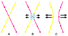 |
Fig. 1. Schematic representation of guide field small-angle reconnection at three different stages. Step A: Two field lines are tilted in opposite directions. Step B: Field lines reconnect in the diffusion region DR, where currents are stronger. Step C: After the reconnection the field line connectivity has changed. The black arrows indicate the outflows. |
A schematic description of the reconnection processes yielding the outflow acceleration is shown in Fig. 1. As drifting magnetic field lines are driven towards one another (A), the magnetic field component perpendicular to the guide field vanishes at the ‘dissipation region’ (DR, where E ⋅ B ≠ 0; Hesse & Schindler 1988; Schindler et al. 1988) and it induces the field connectivity to change (B). The magnetic field reconnects inside DR. The new field lines configuration induces a magnetic tension imbalance which in turn drives field lines to expand outwards (C). Outside of the dissipation region, the plasma is frozen in the field and is accelerated by the slingshot effect caused by the released magnetic tension.
Beyond the work already done with basic models, it remains to be addressed if reconnection collimated outflows can occur in more realistic and dynamic scenarios and whether even in these circumstances they can be detected and observed with current or upcoming instruments. To answer these questions, this work addresses the MHD and forward modelling of an outflow that forms and evolves during an MHD Avalanche (Hood et al. 2016). We investigate the full 3D MHD simulation of an MHD avalanche described in Cozzo et al. (2023b) and check the occurrence of nanojets-like events during the evolution of instability.
2. MHD modelling
We considered the 3D MHD simulation described in Cozzo et al. (2023b) of a MHD avalanche in a kink-unstable, multi-threaded coronal loop system (see also Hood et al. 2016; Reid et al. 2018, 2020). In this case, small angle reconnection episodes result from the turbulent dissipation of the twisted magnetic field during the instability (rather than from regular photospheric motions) directly tilting the field lines, as described in Pagano et al. (2021) and De Pontieu et al. (2022). Two identical magnetic flux tubes are embedded in a stratified solar atmosphere with a 1 MK corona anchored on both sides to a dense and cooler isothermal (104 K) chromosphere. The flux tubes are progressively twisted at different angular velocities by photospheric rotation motions at their footpoints, mirrored with respect to the middle plane (Reale et al. 2016; Cozzo et al. 2023a), in a background magnetic field (Bbkg = 10 Gauss). The time-dependent 3D MHD equations are solved with the Pluto code (Mignone et al. 2007). The computational box has a size of Δx = 16 Mm, Δy = 8 Mm, Δz = 62 Mm. Anomalous magnetic resistivity (η0 = 1014 cm−2 s−1; Hood et al. 2009; Reale et al. 2016) turns on in the corona (T > 104 K) when and where the electric current density, j, exceeds the threshold value jcr = 250 Fr cm−2 s−1. The equations include radiative losses, thermal conduction, and gravity component for a curved flux tube (closed coronal loop).
Due to progressive twisting, the faster rotating flux tube becomes kink-unstable and rapidly fragments into a chaotic system with thin current sheets hosting small-sized impulsive reconnection events. The instability soon propagates to the nearby slower tube, which then evolves in a similar way. The impulsive events cause local heating of the plasma to temperature peaks above 10 MK.
Following the evolution of several magnetic field lines in the aftermath of the MHD avalanche, we identified a few examples of reconnection jets, namely, bundles of magnetic field lines whose evolution follows the patterns described in Fig. 1. We selected one of them as a reference case resulting from the reconnection of two slightly misaligned magnetic filaments carried out by swirling plasma flows.
Figure 2 shows a localised reconnection event with the reference outflow. In the box (62 Mm long, and 8 Mm × 16 Mm cross-section), the atmosphere is stratified, with two chromospheric layers at the top and bottom of the box, and a 50 Mm corona (see Appendix C for details). Field lines in the box are shown in full-3D rendering at three different times and from two different perspectives. They are computed using a fourth-order Runge-Kutta scheme, while the colour is attributed depending on the starting points at the lower photospheric boundary, which move following photospheric twisting. On the left, a view from the top, along the coronal loop axis (z-axis), with a cut at the mid-plane of the box showing in blue the electric field component parallel to the magnetic field. Arrows mark the orientation and strength of the velocity field. On the right, a front view. We draw two reconnecting magnetic field lines. The sites of reconnection are localised as those where the electric field component parallel to the magnetic field is non-zero (E∥; blue spots in the left panels; Hesse & Schindler 1988; Schindler et al. 1988; Reale et al. 2016, see also Fig. A.5 for a full-3D rendering of DR). The velocity field (arrows) illustrates the approaching flows and the collimated outflows diverging from the reconnection site. Movie 1 shows the evolution of the 3D rendering. Initially, the two field lines approach each other, dragged by the chaotic dynamics of the MHD avalanche. The outflowing plasma is then accelerated (second panel) in the dissipation region near the mid-plane centre, namely, where E∥ becomes stronger. Afterwards (third panel) the reconnecting field pushes the plasma outwards where it eventually disperses in the ambient magnetic field.
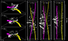 |
Fig. 2. Magnetic reconnection and the outflow. 3D Rendering at three different times since the beginning of the avalanche: Δt = 0 s (lines approaching), Δt = 10 s (lines reconnecting), and Δt = 20 s (new lines detaching). Left column, top view, and cut at the middle plane: Two reconnecting magnetic field lines (marked by yellow and magenta lines among two bundles), reconnection sites (blue spots close to the centre of the plane), and velocity field (white arrows), which shows the collimated outflow departing from the reconnecting lines (see Movie 1). Right row: Same reconnecting lines from a front view (the coronal part of the loop is 50 Mm long; see Movie 2). |
On the right (and in Movie 2), the front view shows the reconnecting lines emphasizing the presence of the guide field, similar to Fig. 1. In the first panel, the reconnecting magnetic field is starting to push the plasma outwards (as emphasised by arrows in a few high velocity spots near the reconnection site). The plasma velocity is mostly perpendicular to the field lines, with a small component along them. This transverse motion is stronger (middle panel) and longer-lasting (third panel) around the middle of the flux tube.
In Fig. 3, we illustrate details of the outflow from the selected reconnection event. The three columns show the velocity component perpendicular to the magnetic field (v⊥), current density, and temperature maps on the mid-plane perpendicular to the z vertical axis and at the same times as in Fig. 2. Movie 3 shows the evolution of the same quantities. The velocity maps, v⊥, emphasise where the plasma is accelerated by the magnetic field tension (as the Lorentz force acts always perpendicular to B) and where instead the plasma drags the magnetic field lines. As expected, the velocity field diverges from the central reconnection site, near x = 0 Mm and y = −1 Mm in two strong, sub-Alfvénic collimated jets. The current maps show an intense sheet in the central reconnection region (middle panel), where the magnetic field clearly reverses its direction on the mid plane. The current density in the sheet exceeds the threshold for dissipation into ohmic heating imposed in the simulation (jcr = 250 Fr cm−2 s−1). The current density is rather weak at the beginning; it intensifies first in the DR, and then in the region around the collimated jets, where it fragments. The dissipation of the reconnection current sheets into heat is confirmed in the temperature maps, with very high values (T ≳ 8 MK), although rapidly decreasing because of the effect of expansion and thermal conduction. The reference outflow itself is actually at these high temperatures, while the density does not exceed n ∼ 109 cm−3 (see Appendix C for more details).
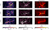 |
Fig. 3. Dynamics of the reconnection outflow. First column: Horizontal mid-plane map of the value of the velocity component perpendicular to the magnetic field at the same three times shown in Fig. 2, i.e. Δt = 0 s (top, current sheet formation), Δt = 10 s (middle, outflow acceleration), and Δt = 20 s (bottom, outflow deceleration). The velocity field in the plane is also shown (arrows). Second column: Horizontal mid-plane map of the current density. The map saturates where the current density exceeds the threshold value for dissipation. The magnetic field in the plane is also shown (arrows). Third column: Horizontal mid-plane map of the temperature. (See Movie 3.) |
The evolution of the reconnection outflow in the midst of the first 300 s from the onset of the instability is shown in Fig. 4. The top panel shows the X-component of the velocity averaged in a box with a size of Δx = 10 Mm, Δy = 4 Mm, Δz = 10 Mm, centred at the origin, as a function of time and x. The plasma is expelled in opposite directions at t ∼ 170 s. At the same time, the current density and the temperature are already high (J > Jcr, second panel, T ∼ 6 MK, third panel) and grow even higher (J ∼ 400, T ∼ 8 MK) in about 10 s. The velocity stays high (≳200 km s−1) for about 30 s, then the jet slows down, the current density dissipates, and the plasma smoothly cools down. We can therefore estimate as ∼30 s the outflow overall duration. The two opposite jets propagate (toward positive and negative  , respectively) with different velocities (as also remarked by the different front slopes in the first panel of Fig. 4). In particular, the bidirectional jet, after Δt = 30 s the reconnection takes place, has expanded by about 10 Mm, with ∼40% of asymmetry between the two parts.
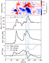 |
Fig. 4. Evolution of the coronal loop plasma in a box containing the reconnection outflow. This reference volume has a size of Δx = 10 Mm, Δy = 4 Mm, Δz = 10 Mm, and is centred at the origin. First panel: X-component of the velocity, averaged along Δy and Δz. Second panel: Maximum temperature in the box. Third panel: Maximum current density in the box. Fourth panel: Total magnetic (solid), kinetic (dashed), and internal (dotted line) energy in the box. |
During the event, a magnetic energy amount of ∼1024 erg is converted into kinetic and internal energy, as shown in the bottom panel of Fig. 4, which shows the evolution of the total magnetic, kinetic, and internal energy over the entire elapsed time of the MHD avalanche in the slab where the outflow dynamics is stronger. This energy budget is compatible with the nanoflare energy predicted by Parker (1988). Within the box, an excess of magnetic energy initially increases, but then rapidly drops (below its initial level) upon activation of the anomalous resistivity. Concurrently, both the thermal and kinetic energies rise at similar rates. Magnetic and thermal energy variations are larger compared to kinetic variations: plasma compression occurs in heating at the expense of the kinetic energy, localised near the centre of the reconnection (where the plasma is accelerated to ∼200 km s−1). The peak in kinetic energy lasts about 30 s, compatibly with the estimated duration of the outflow.
3. Forward modelling and diagnostics
Having described the physical processes that lead to a reconnection outflow in our MHD avalanche simulation, we then tested the detection of such an event. Specifically, the question is whether the outflow can be detected in the EUV band. We considered the 94 Å channel of the Atmospheric Imaging Assembly (AIA; Lemen et al. 2012) on board the Solar Dynamics Observatory (SDO; Pesnell et al. 2012), including the Fe XVIII line emitted at log T ∼ 6.8, and the 108 Å Fe XIX spectral line, formed around log T ∼ 7.0, which will be observed by the forthcoming Multi-slit Solar Explorer (MUSE; De Pontieu et al. 2022; Cheung et al. 2022; see Fig. A.1, which also describes how the synthetic observables are calculated). Both bands are particularly suitable for detecting the outflow with an estimated apex temperature of 8 MK. Appendix A discusses more generally the emission in the six EUV AIA channels and in the three MUSE lines (Fig. A.1). We have also convolved all the emission maps at the original resolution with the instrumental point spread functions (PSFs) and then re-binned them to the instrument pixel size. MUSE PSF is modelled by a Gaussian with FWHM of 0.45″. AIA PSFs are described in, for instance, Poduval et al. (2013).
In the synthetic maps, for a more realistic representation, the flux tube box has been remapped onto a curved loop-like geometry (as in Cozzo et al. 2024). Figure 5 presents how we would detect the emission in the AIA 94 Å channel integrated along a line of sight from a side view of the loops. The model has been remapped and oriented along the selected line-of-sight to maximise the brightness of observational signatures at the apex. The overlapping magnetic field lines at the loop top align the hot plasma along the line-of-sight within a compact region, thereby increasing the emission filling factor.
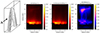 |
Fig. 5. Synthetic maps in the AIA 94 Å channel integrated along a line of sight from a side view of the curved loop system (first panel, exposure time: 9 s). Second panel: In this geometry the top of the loop is high in the image, as shown in the left panel. intensity map in the entire filter band. Third panel: intensity map of the cool component (∼1 MK). Fourth panel: map of the hot (Fe XVIII) component only, after subtracting the middle from the left. |
Under nominal operations, AIA exposure times are up to 2.9 s while the basic time step between snapshots is set to 12 s (Lemen et al. 2012). We assume an exposure time of ∼9 s, to sample an event ≲36 s long (3 × 12 s merged observing windows) from t = 0 s. On the left, we show the emission map in the whole filter band. The low dense and cooler regions of the image are very bright because the filter band includes other intense 1 MK lines (Testa & Reale 2012; Boerner et al. 2014).
The hot outflow emission is already visible, but very faint, high (z ∼ 15 Mm) in the image. To enhance its contrast, we subtracted the cooler component (middle panel of Fig. 5), as obtained from other properly rescaled AIA channels (Reale et al. 2011; Warren et al. 2012; Cadavid et al. 2014; Antolin et al. 2024; see also Appendix A). The result is shown in the right panel. The signature of the jet is the horizontal elongated feature high in the image with a bright spot on the left. The brightest emission (above 50% of the peak) is about 10 Mm long. In this synthetic image, the emission from the hot outflow plasma leads to counts about four times higher than the rest of the image, but nevertheless barely detectable without rebinning.
In Fig. 6, we present the corresponding synthetic emission for the MUSE Fe XIX 108 Å spectral line. We considered an observing mode with a long exposure time of 30 s from t = 0 s. This exposure time envelopes the event completely, although the bulk of the emission is contained in a shorter time, as shown in Fig. 4 and new movies A1 and A2 in Appendix A. The line of sight is the same as in Fig. 5. A 3D rendering of the Fe XIX line emission is shown in Fig. A.4. To improve on the photon statistics closer to the detection level (De Pontieu et al. 2020), we rebinned the map on macro-pixels (0.4″ × 2.7″). The Fe XIX emission map is very similar to the ‘hot’ 94 Å map on the right of Fig. 5 and it highlights the bipolar jet about 500% more clearly, and the hot emission is better isolated in this single line. Also, in this case, the brightest emission (above 50% of the peak) has an elongated shape, about 10 Mm long. The Fe XIX line profile (on the right) is obtained by integrating over an area 5 × 5 Mm2 large and inclined by 10 degrees (schematically highlighted on the right and between the white lines of the mid panel) and using a spectral bin of 80 km s−1 (twice that selected for MUSE De Pontieu et al. 2020). The surface is oriented exactly along the jet and, in this way, we have emphasised the plasma motion along the line of sight. The double-sided jet determines the presence of a clearly defined double peak in the line profile, with peaks located at v ≈ ±200 km s−1 (the Alfvén velocity is about 1000 km s−1).
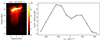 |
Fig. 6. MUSE synthetic map and spectrum (line of sight shown in the Fig. 5). Left: the Fe XIX 108 Å line emission map as in Fig. 5. The emission is integrated over macro-pixels with a size of Δh = 0.28 Mm, Δv = 1.89 Mm (0.4″ × 2.7″) (exposure time: 30 s). Right: Fe XIX line spectrum obtained by integrating the emission along the volume marked in the map on the left (white solid lines, cross-section 5 × 5 Mm). The spectral bin is Δv = 80 km s−1. We account for thermal, non-thermal, and instrumental broadening. |
4. Discussion and conclusions
In this work, we study the serendipitous formation and evolution of a reconnection outflow within the complex background of a coronal flux tube system, which fragments into smaller current sheets with random reconnection episodes. We analyse what kind of detection we might expect both with current instruments, such as the AIA imager, and with the forthcoming MUSE spectrometer. This outflow is the result of a reconnection event, of nanoflare size and comes out perpendicular to the flux tube guide field. It shares therefore many features with observed small-sized jets, named nanojets (Antolin et al. 2021). Previous 3D MHD simulations had addressed the issue of nanojets acceleration with ad hoc setups where field lines are tilted by photospheric motions (Antolin et al. 2021) or where their misalignment is provided from the outset via the initial conditions (Pagano et al. 2021).
Cozzo et al. (2023b) 3D MHD model describes the turbulent, large-scale energy release of multiple magnetic strands within a stratified atmosphere, twisted by footpoint motions. This model provides an excellent opportunity to study the development of jets and possibly nanojets and their possible detection, where they are dispersed in a more realistic situation. In this work, we single out a magnetic reconnection event based on the heating and plasma acceleration that it causes, in the midst of the dynamic and thermally evolving loop structures.
The described event is localised. It involves the thick field lines in Fig. 2, which are driven to cross each other and then detach again with a different topology. Although the configuration is not ideal as in plane parallel cases, there are all signatures of reconnection, including localised heating and perpendicular flows. The E∥ component can be different from zero only in non-ideal plasma conditions (reconnection) and shows very high values halfway down the loop, where the field lines initially cross each other, and much smaller nearby, as emphasised in Fig. A.5 showing the extension of the dissipation region (E∥ ≠ 0) in full 3D. Similarly to Antolin et al. (2021) observations, the jet is observed after the initial MHD avalanche. The outflow event is generated as a result of the formation and dissipation of a current sheet, induced by the chaotic motion of plasma and magnetic field lines during the MHD avalanche. The evolution of the magnetic field lines is remarkably similar to the schematic picture shown in Fig. 1. This event exhibits typical signatures of nanojets as anticipated by previous theoretical and numerical investigations, as well as observations (e.g. Antolin et al. 2021; Sukarmadji et al. 2022). These signatures include typical lateral dimensions of a few thousand kilometres and typical velocities of a few hundreds of kilometres per second. The event also takes place at the top of the loop, as in the case of a number of nanojets observed by Antolin et al. (2021), Sukarmadji et al. (2022), Sukarmadji & Antolin (2024). The magnetic energy released during this event approximates 1024 erg, in agreement with Parker (1988). A significant fraction of this energy is converted into heat, increasing the plasma temperature above 8 MK, while the remaining energy propels the outflow. The jets originate from a localised reconnection event that is the dominant source of plasma heating. Field lines that are overlapping when the system is mapped onto a curved geometry increases the plasma filling factor, influencing the signatures seen in the forward modelling.
Figure 5 shows that the outflow described here is very difficult to detect with present-day capabilities (AIA). Specifically, the AIA 94 Å channel is (in principle) sensitive to such hot plasma, but its detection is made difficult both by the low emission measure of these events and by the presence of a strong cool component in the same filter band. The subtraction of this cool component is an approximation that does not work perfectly and introduces an extra source of noise (on top of photon noise, readout noise, and digitisation noise). The noise related to the subtraction is likely to be significantly higher than the other sources of noise and not properly quantifiable because the individual contributions of the different spectral lines within the broad AIA passbands cannot be determined with a high level of accuracy.
Instead, the MUSE spectrometer is able to isolate the Fe XIX line, which is specifically sensitive to hot plasma only. In consideration of the low emission measure of these events, MUSE thus offers significant advantages over AIA given its sensitivity to the high temperature signal and its capability of detecting the predicted bidirectional Doppler shifts. The characterization of these events will be made even stronger by the peculiar expected bidirectional Doppler shift, which MUSE is tailored to capture.
It is arguable that a stronger magnetic field, or denser loops, can lead to events that would be easier to detect. In fact, higher heat capacity c (due to high averaged density) requires higher magnetic energy budgets, ΔEB, to keep the temperature high; namely, in the Fe XVIII-Fe XIX temperature range, according to
 (1)
(1)
indicating that ΔT ∝ B2/n. With such a scaling pattern, the dissipation of a magnetic field just  times stronger (e.g. ∼30 G) heats up a plasma ten times denser (e.g. ∼1010 cm−3) to million degrees (up to ∼10 MK), attaining a 102 larger emission measure (enough to be easily detected by MUSE at a cadence as short as 10 s). In our simulation, we considered a typical coronal magnetic field strength of 10 G (Long et al. 2017), with a plasma density of about 109 cm−3. Nevertheless, in active regions, magnetic field can exceed 30 G (e.g. Van Doorsselaere et al. 2008; Jess et al. 2016; Brooks et al. 2021), while the density can reach 1010 cm−3 (Reale 2014). In these cases, higher emission is expected and, comparably, shorter exposure times would be needed to single out the outflow jet, making its evolution suitable to be inferred with short-cadence (10 s or less) observing modes (that will be available with MUSE). This scaling needs to be verified to pave the way for the detection of magnetic reconnection in the solar corona.
The event described has all the physical features predicted by the theory of reconnection and shows strong similarities with the theoretical model proposed by Antolin et al. (2021): they both originate from a small-angle reconnection event and share the same orders of magnitude in terms of dimensions, velocity, and duration of the outflow jets. A detailed, physical analysis of the simulated event has also shown many features matching with Antolin et al. (2021) numerical model, including: the distribution and orientation of the velocity field (Fig. 2), the detailed evolution of the magnetic, kinetic, and thermal energy (Fig. 4), and the location and structuring of the dissipation region (Fig. A.5). As a significant deviation from the more idealised model by Antolin et al. (2021), we have shown a bidirectional, but asymmetric jet. Although we have not accounted for magnetic curvature (Pagano et al. 2021) in the simulation, other factors (in particular, local field line braiding and warping and the non-uniform background plasma) effectively make the propagation different on the two sides.
The Antolin et al. (2021) model suggests the role of small-angle magnetic reconnection in accelerating (nano-) jets within a non-vanishing coronal loop magnetic field. This is supported by observational evidence of collimated jets, interpreted as the kinetic counterpart of nanoflare heating. Smoking guns of such nanoflare heating in the tenuous solar corona are difficult to catch because of the small emission measure, and the highly efficient thermal conduction, limiting the visibility of such events to their already short kinetic time scales. In this work, we show that detection of nanoflare jets might be possible with MUSE, even at high temperatures, when the plasma is under-dense and fainter, thanks to the MUSE detailed EUV spectroscopic diagnostics; until now, studies have been restricted to the UV band (De Pontieu et al. 2014).
The onset of the reconnection event is caused by the overlapping of two misaligned bundles of field lines, ultimately brought together by the residual dynamics of the MHD avalanche. This scenario supports the interpretation of Antolin et al. (2021) and Sukarmadji et al. (2022) observations, where it is argued that MHD instabilities can trigger reconnection nanojets.
This study focuses on MHD events occurring around the MHD avalanche triggered by the kink instability. At that time, the impulsive heating events have not been effective in filling the flux tubes with dense plasma yet. In these conditions of tenuous plasma, the heat pulse is effective in determining a steep increase of the local temperature and the outflowing jet is therefore hot as well and faint because of the low density.
This period of the evolution probably represents a relatively short transient in the global evolution of a loop system. Thus, such hot and faint jets are also probably more infrequent and fainter than any of the nanojets observed so far (e.g. Antolin et al. 2021). In a future work, we intend to study the formation and possible detection of reconnection jets in more steady-state conditions, that is, later in the loop evolution, when the flux tubes are filled with denser plasma coming up from the chromosphere, driven by the heating. Cooler and brighter nanojets are therefore expected to occur at a later stage in this more steady-state regime.
Data availability
Movies associated to Figs. 2, 3, A.2, A.3 are available at https://www.aanda.org
Acknowledgments
GC, PP, and FR acknowledge support from ASI/INAF agreement n. 2022-29-HH.0. This work made use of the HPC system MEUSA, part of the Sistema Computazionale per l’Astrofisica Numerica (SCAN) of INAF-Osservatorio Astronomico di Palermo. PT was supported by contract 4105785828 (MUSE) to the Smithsonian Astrophysical Observatory, and by NASA grant 80NSSC20K1272x. BDP and JMS were supported by NASA contract 80GSFC21C0011 (MUSE).
References
- Alfvén, H. 1947, MNRAS, 107, 211 [CrossRef] [Google Scholar]
- Antolin, P., Vissers, G., Pereira, T., van der Voort, L. R., & Scullion, E. 2015, ApJ, 806, 81 [NASA ADS] [CrossRef] [Google Scholar]
- Antolin, P., Pagano, P., Testa, P., Petralia, A., & Reale, F. 2021, Nat. Astron., 5, 54 [NASA ADS] [CrossRef] [Google Scholar]
- Antolin, P., Auchère, F., Winch, E., Soubrié, E., & Oliver, R. 2024, Sol. Phys., 299, 94 [NASA ADS] [CrossRef] [Google Scholar]
- Beveridge, C., Longcope, D., & Priest, E. R. 2003, Sol. Phys., 216, 27 [NASA ADS] [CrossRef] [Google Scholar]
- Boerner, P., Edwards, C., Lemen, J., et al. 2012, Sol. Dyn. Obs., 41 [Google Scholar]
- Boerner, P., Testa, P., Warren, H., Weber, M., & Schrijver, C. 2014, Sol. Phys., 289, 2377 [Google Scholar]
- Brooks, D. H., Warren, H. P., & Landi, E. 2021, ApJ, 915, L24 [NASA ADS] [CrossRef] [Google Scholar]
- Cadavid, A., Lawrence, J., Christian, D., Jess, D., & Nigro, G. 2014, ApJ, 795, 48 [CrossRef] [Google Scholar]
- Cheung, M. C., Martínez-Sykora, J., Testa, P., et al. 2022, ApJ, 926, 53 [NASA ADS] [CrossRef] [Google Scholar]
- Cho, K., Testa, P., De Pontieu, B., & Polito, V. 2023, ApJ, 945, 143 [NASA ADS] [CrossRef] [Google Scholar]
- Cooper, K., Hannah, I. G., Grefenstette, B. W., et al. 2021, MNRAS, 507, 3936 [NASA ADS] [CrossRef] [Google Scholar]
- Cozzo, G., Pagano, P., Petralia, A., & Reale, F. 2023a, Symmetry, 15, 627 [NASA ADS] [CrossRef] [Google Scholar]
- Cozzo, G., Reid, J., Pagano, P., Reale, F., & Hood, A. W. 2023b, A&A, 678, A40 [NASA ADS] [CrossRef] [EDP Sciences] [Google Scholar]
- Cozzo, G., Reid, J., Pagano, P., et al. 2024, A&A, 689, A184 [NASA ADS] [CrossRef] [EDP Sciences] [Google Scholar]
- De Pontieu, B., Title, A., Lemen, J., et al. 2014, Sol. Phys., 289, 2733 [NASA ADS] [CrossRef] [Google Scholar]
- De Pontieu, B., Martínez-Sykora, J., Testa, P., et al. 2020, ApJ, 888, 3 [NASA ADS] [CrossRef] [Google Scholar]
- De Pontieu, B., Testa, P., Martínez-Sykora, J., et al. 2022, ApJ, 926, 52 [NASA ADS] [CrossRef] [Google Scholar]
- Del Zanna, G., Dere, K., Young, P., & Landi, E. 2021, ApJ, 909, 38 [NASA ADS] [CrossRef] [Google Scholar]
- Feldman, U. 1992, Phys. Scr., 46, 202 [CrossRef] [Google Scholar]
- Glesener, L., Krucker, S., Duncan, J., et al. 2020, ApJ, 891, L34 [Google Scholar]
- Gudiksen, B. V., & Nordlund, Å. 2005, ApJ, 618, 1020 [Google Scholar]
- Hesse, M., & Schindler, K. 1988, J. Geophys. Res.: Space Phys., 93, 5559 [NASA ADS] [CrossRef] [Google Scholar]
- Hood, A., Browning, P., & Van der Linden, R. 2009, A&A, 506, 913 [NASA ADS] [CrossRef] [EDP Sciences] [Google Scholar]
- Hood, A. W., Cargill, P., Browning, P., & Tam, K. 2016, ApJ, 817, 5 [NASA ADS] [CrossRef] [Google Scholar]
- Ishikawa, S.-N., Glesener, L., Krucker, S., et al. 2017, Nat. Astron., 1, 771 [NASA ADS] [CrossRef] [Google Scholar]
- Jess, D. B., Reznikova, V. E., Ryans, R. S., et al. 2016, Nat. Phys., 12, 179 [NASA ADS] [CrossRef] [Google Scholar]
- Klimchuk, J. A. 2009, arXiv e-prints [arXiv:0904.1391] [Google Scholar]
- Klimchuk, J. A. 2015, Phil. Trans. Roy. Soc. A: Math. Phys. Eng. Sci., 373, 20140256 [CrossRef] [Google Scholar]
- Klimchuk, J., Patsourakos, S., & Cargill, P. 2008, ApJ, 682, 1351 [NASA ADS] [CrossRef] [Google Scholar]
- Lemen, J. R., Title, A. M., Akin, D. J., et al. 2012, Sol. Phys., 275, 17 [Google Scholar]
- Long, D. M., Valori, G., Pérez-Suárez, D., Morton, R. J., & Vasquez, A. M. 2017, A&A, 603, A101 [NASA ADS] [CrossRef] [EDP Sciences] [Google Scholar]
- Mignone, A., Bodo, G., Massaglia, S., et al. 2007, ApJS, 170, 228 [Google Scholar]
- Pagano, P., Antolin, P., & Petralia, A. 2021, A&A, 656, A141 [NASA ADS] [CrossRef] [EDP Sciences] [Google Scholar]
- Parker, E. N. 1988, ApJ, 330, 474 [Google Scholar]
- Patel, R., & Pant, V. 2022, ApJ, 938, 122 [CrossRef] [Google Scholar]
- Pesnell, W. D., Thompson, B. J., & Chamberlin, P. 2012, The Solar Dynamics Observatory (SDO) (Springer) [Google Scholar]
- Poduval, B., DeForest, C., Schmelz, J., & Pathak, S. 2013, ApJ, 765, 144 [NASA ADS] [CrossRef] [Google Scholar]
- Reale, F. 2014, Liv. Rev. Sol. Phys., 11, 1 [NASA ADS] [Google Scholar]
- Reale, F., Guarrasi, M., Testa, P., et al. 2011, ApJ, 736, L16 [NASA ADS] [CrossRef] [Google Scholar]
- Reale, F., Orlando, S., Guarrasi, M., et al. 2016, ApJ, 830, 21 [CrossRef] [Google Scholar]
- Reid, J., Hood, A. W., Parnell, C. E., Browning, P., & Cargill, P. 2018, A&A, 615, A84 [NASA ADS] [CrossRef] [EDP Sciences] [Google Scholar]
- Reid, J., Cargill, P., Hood, A. W., Parnell, C. E., & Arber, T. D. 2020, A&A, 633, A158 [NASA ADS] [CrossRef] [EDP Sciences] [Google Scholar]
- Schindler, K., Hesse, M., & Birn, J. 1988, J. Geophys. Res.: Space Phys., 93, 5547 [NASA ADS] [CrossRef] [Google Scholar]
- Sukarmadji, A. R. C., & Antolin, P. 2024, ApJ, 961, L17 [NASA ADS] [CrossRef] [Google Scholar]
- Sukarmadji, A. R. C., Antolin, P., & McLaughlin, J. A. 2022, ApJ, 934, 190 [NASA ADS] [CrossRef] [Google Scholar]
- Testa, P., & Reale, F. 2012, ApJ, 750, L10 [NASA ADS] [CrossRef] [Google Scholar]
- Testa, P., & Reale, F. 2023, in Handbook of X-ray and Gamma-ray Astrophysics, eds. C. Bambi, & A. Santangelo, 134 [Google Scholar]
- Testa, P., De Pontieu, B., Martínez-Sykora, J., et al. 2013, ApJ, 770, L1 [NASA ADS] [CrossRef] [Google Scholar]
- Testa, P., De Pontieu, B., Allred, J., et al. 2014, Science, 346, 1255724 [Google Scholar]
- Testa, P., Polito, V., & De Pontieu, B. 2020, ApJ, 889, 124 [Google Scholar]
- Van Doorsselaere, T., Nakariakov, V. M., Young, P. R., & Verwichte, E. 2008, A&A, 487, L17 [NASA ADS] [CrossRef] [EDP Sciences] [Google Scholar]
- Vekstein, G. 2009, A&A, 499, L5 [NASA ADS] [CrossRef] [EDP Sciences] [Google Scholar]
- Viall, N. M., & Klimchuk, J. A. 2011, ApJ, 738, 24 [Google Scholar]
- Warren, H. P., Winebarger, A. R., & Brooks, D. H. 2012, ApJ, 759, 141 [NASA ADS] [CrossRef] [Google Scholar]
- Wright, P. J., Hannah, I. G., Grefenstette, B. W., et al. 2017, ApJ, 844, 132 [NASA ADS] [CrossRef] [Google Scholar]
Appendix A: Details on forward modelling
To make a comparison with the familiar semicircular shape of coronal loops, the original simulation outputs were remapped and interpolated onto a new cartesian grid. In this process, the initially straight coronal section of the domain was curved into a half-cylinder shell with a characteristic radius of R = L/π with L = 50 Mm, the loop’s coronal length. On the other hand, the chromospheric layers were modelled as two parallel parallelepipeds, as described in Cozzo et al. (2024).
To remap on observation-like images, we computed line emission I0 from the pixel i, j, by integrating cells intensity Fi, j, k (in units of ph s−1 pix−1) along the line of sight (as in De Pontieu et al. 2022; Cozzo et al. 2024):
 (A.1)
(A.1)
with
 (A.2)
(A.2)
where ne is the free electron density, Λ(T) is the instrument temperature response function, and Δz is the cell width. Instrument temperature response functions are calculated using CHIANTI 10 (Del Zanna et al. 2021) with the CHIANTI ionization equilibrium, coronal element abundances (Feldman 1992), assuming a constant electron density of 109 cm−3, and no absorption considered.
In Fig. A.1, we show the temperature response functions Λ(T) of the three MUSE EUV lines: Fe IX 171 Å, Fe XV 285 Å, and Fe XIX 108 Å (top panel, De Pontieu et al. 2020); and of the six AIA EUV channels at 94 Å, 131 Å, 171 Å, 193 Å, 211 Å, and 335 Å, respectively (mid panel, Boerner et al. 2012).
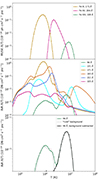 |
Fig. A.1. Temperature response functions Λi(T) for the AIA and MUSE channels. Top: MUSE spectrometer lines: Fe IX 171 Å, Fe XV 284 Å, and Fe XIX 108 Å. Middle: AIA 94 Å (containing Fe XVIII line), 131 Å, 171 Å, 193 Å, 211 Å, and 335 Å channels. Bottom: expected response function of the 94 Å AIA channel (black line) after the subtraction of the cold component (dotted line) obtained by combination of 131 Å, 171 Å, 193 Å, 211 Å, and 335 Å AIA channels from the total one (light green). |
In Fig. A.2, we show synthetic AIA emission maps from 9 s effective exposures. Each panel shows the side view of the intensity distribution integrated over the entire filter band of the six EUV channels in Fig. A.1. Emission in 131 Å, and 171 Å channels is dominated by a relatively cool (≲1 MK) plasma component just above the transition region (< 5 Mm in height); 193 Å, 211 Å, and 335 Å channels show evidence of warmer plasma (2 − 4 MK) at intermediate height (≳5 Mm). A faint feature from hot (≳5 MK) plasma shows up around the loop top (∼15 Mm) in the 94 Å channel (containing the ‘hot’ Fe XVIII line), although most of the intensity comes from the cooler plasma background. Movie A1 shows the evolution of the coronal loop emission as imaged by the six AIA channels (Fig A.1), and contributing to the integrated emission of Fig. A.2. The atmosphere appears roughly steady in all the channels, with some noisy gleaming in the lower, cooler corona, and slow variations in the atmospheric structuring of the warm plasma at intermediate heights. Only the hot plasma jet at the loop top evolves dynamically, and expands outward until its emission vanishes in the background.
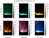 |
Fig. A.2. Synthetic maps of AIA emission integrated along a line of sight from a side view of the curved loop system for 94 Å, 131 Å, 171 Å, 193 Å, 211 Å, and 335 Å channels, respectively (see Movie A1). |
 |
Fig. A.3. Synthetic maps of MUSE emission integrated along a line of sight from a side view of the curved loop system for the Fe IX 171 Å, Fe XV 284 Å, and Fe XIX 108 Å lines, respectively (see Movie A2). |
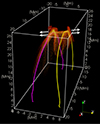 |
Fig. A.4. 3D rendering of the MUSE Fe XIX line emission at t = 10 s. In the 3D box, we show two field lines remapped in curved geometry for reference. The arrow point in the direction of the jet propagation. |
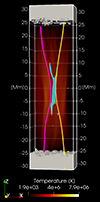 |
Fig. A.5. 3D rendering of the analysed magnetic reconnection region. Field lines are the same as in the second panel of Fig. 2 (t = 10 s). The temperature (red) is shown in the background. Here we also show the diffusion region DR (pale blue, Fig. 1) defined by the region where where E ⋅ B ≠ 0. The solid blocks at the top and bottom are the footpoints in the chromosphere. |
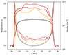 |
Fig. A.6. Plasma vertical stratification: temperature (solid line) and density (dashed) along a 1-pixel column crossing the jet centre (coordinates: x = y = 0 Mm) before the instability (black line) and at times t = 0 s (orange) Δt = 10 s (red), t = 20 s (dark-red) from the ignition of the jet. |
The synthetic emission as sampled by the three MUSE channels (Fig. A.1) is shown in Fig. A.3. We assumed a 30 s exposure time and line of sight from a side view of the curved loop. MUSE lines (Fe IX 171Å, Fe XV 284Å, and Fe XIX 108Å) detect plasma emitting mostly around ∼1 MK, ∼2 MK, and ∼10 MK plasma, respectively. In particular, the Fe IX line is emitted mostly at the loop footpoints; in the Fe XV line we see the bulk of the loop; the Fe XIX line shows a transient brightening around the loop apex. Similarly to Movie A1, Movie A2 shows the evolution of the loop in the MUSE lines when the jet is visible. No evidence of the jet is found in the cooler MUSE channels. In the hot 108Å line, the bright feature stretches into a strongly elongated structure.
In Fig. A.4, the 3D rendering in curved geometry clearly shows the jet emission in the MUSE Fe XIX channel at 108 Å to be perpendicular to the guide field (represented by the drawn field lines). This can be compared to observed nanojets as in Antolin et al. (2021). Specifically, the brighter plasma (yellow volume) envelopes the jet at the loop top, but “tails” of hot plasma (redder parts), propagating along the field, also stand out in the EUV Fe XIX line emission. They form because thermal conduction efficiently spreads heat from the reconnection site.
Figure A.1 shows also the temperature response function Λ(T) for the AIA filter at 94 Å (light green curve; Boerner et al. 2012) The figure also shows the same response function after subtraction of the cool component (dotted line) obtained by a combination of the other AIA responses (131 Å, 171 Å, 193 Å, 211 Å, and 335 Å). More in particular, we derived the background-subtracted emission maps  for the AIA filter at 94 Å as follows:
 (A.3)
(A.3)
where I0bkg is the cooler background image we obtain from the other AIA filters (Reale et al. 2011; Warren et al. 2012; Cadavid et al. 2014; Antolin et al. 2024). In this way we manage to isolate better the emission in the hot Fe XVIII line.
To compute the line profiles (Fe XIX line), we assumed at fixed temperature, density, plasma velocity, and a Gaussian profile,
![Mathematical equation: $$ \begin{aligned} f_{\mathrm{cell} } (v) = \frac{F_{\mathrm{cell} }}{\sqrt{2 \pi \sigma _T^2}} \exp { \left[ -\left(\frac{v - v_{\mathrm{cell} }}{\sigma _T} \right)^2 \right] } ,\end{aligned} $$](/articles/aa/full_html/2025/03/aa52426-24/aa52426-24-eq8.gif) (A.4)
(A.4)
where  is the thermal broadening, mFe is the Fe atomic mass, and vcell is the plasma velocity parallel to the line of sight in a single cell. MUSE Fe XIX spectral bin is Δv = 40 km s−1 (De Pontieu et al. 2020). We assumed a spectral bin twice as large, Δv = 80 km s−1, to increase the photon counts. We account for both thermal and non-thermal broadening.
Finally, we rebinned MUSE Fe XIX observables on macropixels (0.4″ × 2.7″) that collect more photon counts, namely, which are closer to the detection level (De Pontieu et al. 2020). Here, the AIA 94 Å channel intensity is shown with the original pixel size (0.6″ × 0.6″).
Appendix B: Other 3D renderings
Figure A.5 shows the 3D rendering of the diffusion region (in solid cyan; see also Fig. 1) between two reconnecting field lines at t = 10 s (as in Fig. 2). The thin diffusion region develops where the field lines meet and reconnect (i.e. close to the box centre). It is elongated and oriented along the guide field, with short ‘branches’ inclined with the magnetic field bundles to form an ‘X shape’. Hot coronal plasma is in the proximity of the reconnection site. Field lines are embedded in the chromosphere, shown by solid blocks at the top and bottom sides of the box.
Appendix C: Atmospheric stratification
The simulated solar atmosphere consists of a chromospheric and a coronal column separated by a thin transition region. Specifically, field-aligned gravity, thermal conduction, optically thin radiative losses, heating by anomalous magnetic resistivity, and background heating structures a 5 Mm long coronal loop, while its chromospheric footpoints are ∼6 Mm wide each and 104 K hot (Reale et al. 2016; Cozzo et al. 2023b).
Figure A.6 shows the temperature and density stratification along a column of pixels passing through the jet centre (coordinates: x = y = 0 Mm). Before the avalanche (black curve), the atmosphere is initially tenuous (n ∼ 108 cm−3) and cold (T ≲ 1 MK). After the instability, when the jet is formed, the plasma is rapidly heated (solid, orange line, t = 0 s) and the temperature rises up to 10 MK (red line, t = 10 s), and subsequently cools down (orange line, t = 20 s). The density (dashed lines) increases as well, approaching, but never exceeding, n ∼ 109 cm−3.
All Figures
|
Fig. 1. Schematic representation of guide field small-angle reconnection at three different stages. Step A: Two field lines are tilted in opposite directions. Step B: Field lines reconnect in the diffusion region DR, where currents are stronger. Step C: After the reconnection the field line connectivity has changed. The black arrows indicate the outflows. |
| In the text | |
|
Fig. 2. Magnetic reconnection and the outflow. 3D Rendering at three different times since the beginning of the avalanche: Δt = 0 s (lines approaching), Δt = 10 s (lines reconnecting), and Δt = 20 s (new lines detaching). Left column, top view, and cut at the middle plane: Two reconnecting magnetic field lines (marked by yellow and magenta lines among two bundles), reconnection sites (blue spots close to the centre of the plane), and velocity field (white arrows), which shows the collimated outflow departing from the reconnecting lines (see Movie 1). Right row: Same reconnecting lines from a front view (the coronal part of the loop is 50 Mm long; see Movie 2). |
| In the text | |
|
Fig. 3. Dynamics of the reconnection outflow. First column: Horizontal mid-plane map of the value of the velocity component perpendicular to the magnetic field at the same three times shown in Fig. 2, i.e. Δt = 0 s (top, current sheet formation), Δt = 10 s (middle, outflow acceleration), and Δt = 20 s (bottom, outflow deceleration). The velocity field in the plane is also shown (arrows). Second column: Horizontal mid-plane map of the current density. The map saturates where the current density exceeds the threshold value for dissipation. The magnetic field in the plane is also shown (arrows). Third column: Horizontal mid-plane map of the temperature. (See Movie 3.) |
| In the text | |
|
Fig. 4. Evolution of the coronal loop plasma in a box containing the reconnection outflow. This reference volume has a size of Δx = 10 Mm, Δy = 4 Mm, Δz = 10 Mm, and is centred at the origin. First panel: X-component of the velocity, averaged along Δy and Δz. Second panel: Maximum temperature in the box. Third panel: Maximum current density in the box. Fourth panel: Total magnetic (solid), kinetic (dashed), and internal (dotted line) energy in the box. |
| In the text | |
|
Fig. 5. Synthetic maps in the AIA 94 Å channel integrated along a line of sight from a side view of the curved loop system (first panel, exposure time: 9 s). Second panel: In this geometry the top of the loop is high in the image, as shown in the left panel. intensity map in the entire filter band. Third panel: intensity map of the cool component (∼1 MK). Fourth panel: map of the hot (Fe XVIII) component only, after subtracting the middle from the left. |
| In the text | |
|
Fig. 6. MUSE synthetic map and spectrum (line of sight shown in the Fig. 5). Left: the Fe XIX 108 Å line emission map as in Fig. 5. The emission is integrated over macro-pixels with a size of Δh = 0.28 Mm, Δv = 1.89 Mm (0.4″ × 2.7″) (exposure time: 30 s). Right: Fe XIX line spectrum obtained by integrating the emission along the volume marked in the map on the left (white solid lines, cross-section 5 × 5 Mm). The spectral bin is Δv = 80 km s−1. We account for thermal, non-thermal, and instrumental broadening. |
| In the text | |
|
Fig. A.1. Temperature response functions Λi(T) for the AIA and MUSE channels. Top: MUSE spectrometer lines: Fe IX 171 Å, Fe XV 284 Å, and Fe XIX 108 Å. Middle: AIA 94 Å (containing Fe XVIII line), 131 Å, 171 Å, 193 Å, 211 Å, and 335 Å channels. Bottom: expected response function of the 94 Å AIA channel (black line) after the subtraction of the cold component (dotted line) obtained by combination of 131 Å, 171 Å, 193 Å, 211 Å, and 335 Å AIA channels from the total one (light green). |
| In the text | |
|
Fig. A.2. Synthetic maps of AIA emission integrated along a line of sight from a side view of the curved loop system for 94 Å, 131 Å, 171 Å, 193 Å, 211 Å, and 335 Å channels, respectively (see Movie A1). |
| In the text | |
|
Fig. A.3. Synthetic maps of MUSE emission integrated along a line of sight from a side view of the curved loop system for the Fe IX 171 Å, Fe XV 284 Å, and Fe XIX 108 Å lines, respectively (see Movie A2). |
| In the text | |
|
Fig. A.4. 3D rendering of the MUSE Fe XIX line emission at t = 10 s. In the 3D box, we show two field lines remapped in curved geometry for reference. The arrow point in the direction of the jet propagation. |
| In the text | |
|
Fig. A.5. 3D rendering of the analysed magnetic reconnection region. Field lines are the same as in the second panel of Fig. 2 (t = 10 s). The temperature (red) is shown in the background. Here we also show the diffusion region DR (pale blue, Fig. 1) defined by the region where where E ⋅ B ≠ 0. The solid blocks at the top and bottom are the footpoints in the chromosphere. |
| In the text | |
|
Fig. A.6. Plasma vertical stratification: temperature (solid line) and density (dashed) along a 1-pixel column crossing the jet centre (coordinates: x = y = 0 Mm) before the instability (black line) and at times t = 0 s (orange) Δt = 10 s (red), t = 20 s (dark-red) from the ignition of the jet. |
| In the text | |
Current usage metrics show cumulative count of Article Views (full-text article views including HTML views, PDF and ePub downloads, according to the available data) and Abstracts Views on Vision4Press platform.
Data correspond to usage on the plateform after 2015. The current usage metrics is available 48-96 hours after online publication and is updated daily on week days.
Initial download of the metrics may take a while.