| Issue |
A&A
Volume 689, September 2024
|
|
|---|---|---|
| Article Number | A184 | |
| Number of page(s) | 13 | |
| Section | The Sun and the Heliosphere | |
| DOI | https://doi.org/10.1051/0004-6361/202450644 | |
| Published online | 16 September 2024 | |
Coronal energy release by MHD avalanches
II. EUV line emission from a multi-threaded coronal loop
1
Dipartimento di Fisica & Chimica, Universitá di Palermo, Piazza del Parlamento 1, 90134 Palermo, Italy
2
School of Mathematics and Statistics, University of St Andrews, St Andrews, Fife KY16 9SS, UK
3
INAF-Osservatorio Astronomico di Palermo, Piazza del Parlamento 1, 90134 Palermo, Italy
4
Harvard–Smithsonian Center for Astrophysics, 60 Garden St., Cambridge, MA 02193, USA
5
Lockheed Martin Solar & Astrophysics Laboratory, 3251 Hanover St, Palo Alto, CA 94304, USA
6
Rosseland Centre for Solar Physics, University of Oslo, PO Box 1029 Blindern 0315 Oslo, Norway
7
Institute of Theoretical Astrophysics, University of Oslo, PO Box 1029 Blindern 0315 Oslo, Norway
8
Bay Area Environmental Research Institute, NASA Research Park, Moffett Field, CA 94035, USA
Received:
7
May
2024
Accepted:
5
June
2024
Abstract
Context. Magnetohydrodynamic (MHD) instabilities, such as the kink instability, can trigger the chaotic fragmentation of a twisted magnetic flux tube into small-scale current sheets that dissipate as aperiodic impulsive heating events. In turn, the instability could propagate as an avalanche to nearby flux tubes and lead to a nanoflare storm. Our previous work was devoted to related 3D MHD numerical modeling, which included a stratified atmosphere from the solar chromosphere to the corona, tapering magnetic field, and solar gravity for curved loops with the thermal structure modelled by plasma thermal conduction, along with optically thin radiation and anomalous resistivity for 50 Mm flux tubes.
Aims. Using 3D MHD modeling, this work addresses predictions for the extreme-ultraviolet (EUV) imaging spectroscopy of such structure and evolution of a loop, with an average temperature of 2–2.5 MK in the solar corona. We set a particular focus on the forthcoming MUSE mission, as derived from the 3D MHD modeling.
Methods. From the output of the numerical simulations, we synthesized the intensities, Doppler shifts, and non-thermal line broadening in 3 EUV spectral lines in the MUSE passbands: Fe IX 171 Å, Fe XV 284 Å, and Fe XIX 108 Å, emitted by ∼1 MK, ∼2 MK, and ∼10 MK plasma, respectively. These data were detectable by MUSE, according to the MUSE expected pixel size, temporal resolution, and temperature response functions. We provide maps showing different view angles (front and top) and realistic spectra. Finally, we discuss the relevant evolutionary processes from the perspective of possible observations.
Reults. We find that the MUSE observations might be able to detect the fine structure determined by tube fragmentation. In particular, the Fe IX line is mostly emitted at the loop footpoints, where we might be able to track the motions that drive the magnetic stressing and detect the upward motion of evaporating plasma from the chromosphere. In Fe XV, we might see the bulk of the loop with increasing intensity, with alternating filamentary Doppler and non-thermal components in the front view, along with more defined spots in the topward view. The Fe XIX line is very faint within the chosen simulation parameters; thus, any transient brightening around the loop apex may possibly be emphasized by the folding of sheet-like structures, mainly at the boundary of unstable tubes.
Conclusions. In conclusion, we show that coronal loop observations with MUSE can pinpoint some crucial features of MHD-modeled ignition processes, such as the related dynamics, helping to identify the heating processes.
Key words: Sun: corona / Sun: UV radiation
Corresponding author; This email address is being protected from spambots. You need JavaScript enabled to view it. .
© The Authors 2024
 Open Access article, published by EDP Sciences, under the terms of the Creative Commons Attribution License (https://creativecommons.org/licenses/by/4.0), which permits unrestricted use, distribution, and reproduction in any medium, provided the original work is properly cited.
This article is published in open access under the Subscribe to Open model. This email address is being protected from spambots. You need JavaScript enabled to view it. to support open access publication.
1. Introduction
The solar corona consists of plasma confined by and interacting with the coronal magnetic field (Vaiana et al. 1973; Testa & Reale 2023). Frequently, it appears as arch-shaped, dense, and bright filamentary structures, confined by the magnetic field, and known as coronal loops (e.g., Reale 2014). These loops are at temperatures above one million Kelvin, however, the explanation behind this still remains a long-standing problem (Grotrian 1939; Edlén 1943; Peter & Dwivedi 2014).
Presently, there is a general acknowledgment of the magnetic field’s predominant role as the primary source of heating energy (Alfvén 1947; Parker 1988, and see also reviews by e.g., Klimchuk 2015; Testa & Reale 2023 and references therein). In particular, to address the coronal heating problem, two main classes of mechanisms have been envisaged: one involves the dissipation of stored magnetic stresses, referred to as DC heating and the other involves the damping of magnetohydrodynamic (MHD) waves, known as AC heating (Parnell & De Moortel 2012; Zirker 1993).
Overall, DC heating involves magnetic energy storage and impulsive, widespread release. In fact, as the magnetic field evolves over time, energy builds up in the solar corona, which can later be converted into thermal energy. In particular, turbulent photospheric motions cause coronal magnetic field lines to twist and tangle with each other, leading to the inevitable growth of magnetic stresses (Parker 1988; Klimchuk 2015). As a consequence of the ongoing stirring of plasma in the photosphere, caused by magnetoconvection, the magnetic field lines (forming coronal loops) are expected to exhibit intricate braiding patterns at extremely fine resolutions, smaller than an arcsecond (Klimchuk 2009; Cirtain et al. 2013). Parker envisaged that this ongoing process would ultimately give rise to widespread formation of tangential discontinuities in the magnetic field and small-scale current sheets within the solar corona. These discontinuities would serve as sites for magnetic reconnection events, leading to the release of small amounts of energy, on the order of 1024 erg in what are called ‘nanoflares’ (Parker 1988).
Although photospheric plasma induces slow and local dragging of magnetic field lines at loop “footpoints”, according to Parker’s theory, magnetic energy release in the large scale coronal environment is expected to occur through impulsive and widespread heating events. One potential heating mechanism that can produce rapid surges of energy release from the slow, continual driving of boundary motions is the avalanche model (Hood et al. 2016). In this model, a localized MHD instability, within a single strand of a coronal loop, results in widespread disruption as neighboring strands become affected by the propagating disturbance. This mechanism offers a promising explanation for the complex interplay between slow and fast processes in coronal energy release.
In particular, as turbulent motion induces twisting of the loop’s magnetic field lines, such flux tubes can become susceptible to the kink instability (Hood & Priest 1979; Hood et al. 2009), resulting in the release of magnetic energy through sudden, widespread heating events. The initial helical current sheet progressively fragments in a turbulent way into smaller scale sheets. The turbulent dissipation of the magnetic structure into small-scale current sheets occurs as a sequence of aperiodic, impulsive heating events, similar to nanoflare storms.
This is the case of the numerical experiments described in Tam et al. (2015), Hood et al. (2016), and Reid et al. (2018, 2020), where strongly twisted multi-threaded coronal loops undergo kink instabilities and dissipate energy through a turbulent cascade of current sheets. In these cases, purely coronal loops were taken into account, without considering the interaction with the underlying chromospheric layer. In particular, when multiple magnetic strands coexist within the same coronal loop, a single unstable magnetic strand could disrupt the stable strands nearby and trigger a global dissipation of magnetic energy, through a domino-effect called an “MHD avalanche” (Hood et al. 2016). Recently, Cozzo et al. (2023b) addressed the problem of MHD avalanches by means of non-ideal MHD modeling and fully 3D numerical simulations. They considered a stratified solar atmosphere (including the chromospheric layer, transition region, and lower corona), where multiple interacting coronal loop strands are progressively twisted and eventually become unstable. They confirm that avalanches are a viable mechanism for the storage and release of magnetic energy in coronal loops, as a result of photospheric motions in a more realistic solar atmosphere.
The Multi-slit Solar Explorer (De Pontieu et al. 2020, 2022; Cheung et al. 2022, MUSE) is an upcoming NASA MIDEX mission, featuring a multi-slit extreme-ultraviolet (EUV) spectrometer and an EUV context imager, planned for launch in 2027. MUSE is designed to offer high spatial and temporal resolution for spectral and imaging observations of the solar corona. One of the MUSE science goals is to advance the understanding of the heating mechanisms in the corona of both the quiet Sun and active regions, as well as of the physical processes governing dynamic phenomena like flares and eruptions. MUSE will provide fine spatio-temporal coverage of coronal dynamics, as well as wide field of view (FoV) observations, offering valuable insights into the physics of the solar atmosphere. In particular, it will obtain high resolution spectra (≈0.38″), with wide angular coverage (≈156″ × 170″; resembling the typical size of an active region) and 12 s cadence. With its 35-slit spectrometer, MUSE will provide spectral observations, with unprecedented combination of cadence and spatial coverage, in different EUV passbands dominated by strong lines formed over a wide temperature range, enabling the testing of state-of-the-art models related to coronal heating, solar flares, and coronal mass ejections.
The main EUV lines in the MUSE passbands (171 Å Fe IX, 284 Å Fe XV, and 108 Å Fe XIX and Fe XXI), are listed in Table 1 (for details, see De Pontieu et al. 2020, 2022). Here, we focus on the new spectroscopic diagnostics provided by MUSE, but of course the findings can be extended to observations with other imaging and spectroscopic solar instruments observing at similar wavelengths, for instance, SDO/AIA (Pesnell et al. 2012; Lemen et al. 2012), Hinode/EIS (Culhane et al. 2007; Tsuneta et al. 2008), and the forthcoming Solar-C/EUVST (Shimizu et al. 2019).
MUSE spectrometer emission lines.
To make meaningful predictions that can then be compared with solar observations, two critical developments are essential. Firstly, the modeling approach must encompass crucial physical components, including the thermodynamic response of atmosphere, to derive realistic observational outcomes. Secondly, observational techniques must achieve sufficient temporal and spatial resolution within the pertinent spectral bands. The synergistic comparison between coronal observations and synthetic plasma diagnostics from numerical simulations can, on the one hand, significantly improve our interpretative power on real observational data. On the other hand, it can also help to refine the solar coronal modeling process.
This study focuses on extending the plasma diagnostics of the MHD avalanche model introduced by Cozzo et al. (2023b) to observations with the forthcoming MUSE spectrograph. Although our analysis addresses plasma diagnostics from the MUSE spectrometer, the present work has a more general application to the plasma emission at representative coronal temperatures.
We extracted plasma diagnostics from a full 3D MHD simulation of a flaring coronal loop undergoing an MHD avalanche, as described in Cozzo et al. (2023b). In particular, we modeled the response of the MUSE spectrometer by using our simulated plasma output to synthesize line emission, intensity maps, Doppler shifts and non-thermal line widths, across the three spectral channels available with the instrument.
In Section 2, the MHD avalanche model from which observables are synthesized is briefly presented. In Section 3, we describe the method employed to extract these synthetic observables. In Section 4, we present our results. In Section 5, we discuss the results and give our conclusions.
2. Model
As described in Cozzo et al. (2023b), we modeled a magnetized solar atmosphere in a 3D cartesian box of size, −xM < x < xM, −yM < y < yM, and −zM < z < zM, where xM = 2yM = 8.5 × 108 cm, and zM = 3.1 × 109 cm with PLUTO Code (Mignone et al. 2007).
The background atmosphere consists of a chromospheric and a coronal column separated by a thin transition region. Specifically, in the corona, two flux tubes interact, each with a length 50 Mm and initial temperature of approximately 106 K, while the two chromospheric layers are ∼6 Mm wide each and 104 K hot. The transition region, ≈1 Mm wide, is artificially broadened using Linker–Lionello–Mikić method (Linker et al. 2001; Lionello et al. 2009; Mikic et al. 2013).
The loop’s magnetic field is line-tied to the photospheric boundaries, at the opposite sides of the domain. The coronal loop is rooted to the chromosphere by its footpoints and it expands approaching the corona. Radiative losses and thermal conduction drain internal energy from the corona while a uniform and static heating prevents the atmosphere from cooling down and maintains the corona in steady conditions.
Two rotational motions at the footpoints twist each of the flux tubes. The two rotating regions have the same radius (R ≈ 1 Mm), but one has an angular velocity that is higher than the other by 10% (≈10−3 rad s−1 vs. ≈0.9 × 10⁻³ rad s−1), so that the faster strand becomes unstable first, triggering the avalanche process. As a reference time, deemed t = 0 s, we chose the time when the faster flux tube is nearly kink-unstable. Then, this kink-unstable tube rapidly disrupts the other one (t = 285 s). A 3D rendering of the two flux tubes and of their interaction as a result of the instability is shown in Fig. 1. Here, we focus on the evolution after the first kink instability.
 |
Fig. 1. 3D rendering of the magnetic field lines inside the box at times (from left to right): t = 0 s (initial condition), 180 s, (first loop disruption), and 500 s. The change in the field line connectivity during the evolution of the MHD cascade is emphasized by the colors. |
The instability makes the initially monolithic flux tubes fragment into a turbulent structure of thinner strands. The initially helical current sheet fragments into smaller and smaller currents sheets, which dissipate by magnetic reconnection and are responsible for a sequence of aperiodic impulsive heating events.
The left panels of Fig. 2 shows a cross-section at the mid-plane of the computational box at time t = 180 s, after the beginning of the instability, when the flux tube on the left (x < 0) has already become unstable and fragmented, and is about to trigger the instability of the flux tube on the right (x > 0). The current density map (top left panel) clearly shows on the left the thin, intense current sheets, around which magnetic reconnection occurs and magnetic energy dissipates. On the right of the map, we see the other flux tube, still not involved in the instability. In the lower-left panel, we show the magnetic field intensity: where the left-hand flux tube was, the field is more blurred, dispersed, and irregularly distributed as a consequence of the instability. The flux tube on the right is still compact and coherent. The twisting is emphasized by the vector field of the component parallel to the plane. The right panels of Fig. 2 show the same quantities as do those on the left, but at a later time (t = 285 s), when the flux tube on the right has also been disrupted.
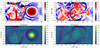 |
Fig. 2. MHD avalanche 2D snapshots. Upper panels. Horizontal cuts of the current density across the mid plane at time t = 180 s (left) and t = 285 s (right). The green contours encloses the regions of the domain heated by ohmic dissipation. Lower panels. Horizontal cuts of the magnetic field across the mid-plane at the same snapshot-times as before. The vector field is included. |
3. Methods: Forward modeling
The emission intensity I (Boerner et al. 2012) from the modelled (optically thin) plasma expected to be measured with MUSE is:
 (1)
(1)
where Λf(T) is the temperature response function per unit pixel for the line, f, and  is the differential emission measure (with ne the free electron density). Then, Λf(T) combines the emission properties of the plasma with the response of the instrument:
 (2)
(2)
where G(λ, T) is the plasma contribution function, Rf(λ) is the spectral response of the f-th instrument channel, and Apix is the area of a single MUSE pixel (0.167″ × 0.4″). The temperature response functions for the three MUSE channels are shown in Fig. 3. They are calculated using CHIANTI 10 (Del Zanna et al. 2021) with the CHIANTI ionization equilibrium, coronal element abundances (Feldman 1992), assuming a constant electron density of 109 cm−3, and no absorption considered. Each curve is multiplied by a factor to convert photons into data-numbers (DN). Each curve peaks approximately at the temperatures listed in table 1. The intensity of a single cell, labeled in the numerical grid by the indices i, j, k, in units of DN s−1 pix−1, is equal to (De Pontieu et al. 2022):
 (3)
(3)
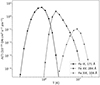 |
Fig. 3. Response function Λi(T) for the three MUSE emission lines (Fe IX, Fe XV, and Fe XIX) as a function of temperature. |
with  , where ρ is the mass density, mH is the hydrogen mass, and Δz is the cell extent along a specific line of sight (LoS), such as
  . We assume a Gaussian profile for each line, at a fixed temperature and density. Therefore, each cell, with a local velocity of vi, j, k along the LoS, contributes to the overall line spectrum with the following single-cell line profile:
![Mathematical equation: $$ \begin{aligned} f_{i,j,k} (v) = \frac{F_{i,j,k}}{\sqrt{2 \pi \sigma _T^2}} \exp { \left[ -\left(\frac{v - v_{i,j,k}}{\sigma _T} \right)^2 \right] } ,\end{aligned} $$](/articles/aa/full_html/2024/09/aa50644-24/aa50644-24-eq7.gif) (4)
(4)
where
 (5)
(5)
is the thermal broadening and mFe is the iron atomic mass, since we will look only at iron lines. The synthetic instrument response, namely, the integrated emission along the LoS is computed as:
 (6)
(6)
MUSE will measure the line profiles, from which we can derive the line Doppler shifts and the line widths. We can compute the first moment of the velocity distribution along the LoS:
 (7)
(7)
which can be compared to the Doppler shifts measured along the LoS. We can derive the non-thermal contribution to the line width (measured after subtracting the thermal line broadening, σT, and instrumental broadening) from the second moment of the velocity:
 (8)
(8)
4. Results
To replicate the typical, semicircular, coronal loops shape better, the original data have been remapped and interpolated onto a new cartesian grid. The method is discussed in Appendix A. Fig. 4 shows the 3D rendering of magnetic field lines in the new geometry, at the same snapshot times used for Fig. 1. Magnetic field lines are color-coded according to the plasma temperature, ranging from 104 K in the chromosphere (blue-layer in the lower part of the box) up to 4 × 10⁶ K in the upper corona. The sequence clearly shows that both flux tubes are progressively heated from about 1 MK to more than 2 MK in the coronal part.
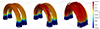 |
Fig. 4. 3D rendering of the magnetic field lines inside the box at the same times shown in Fig. 1. Magnetic field lines are color-coded according to the plasma temperature. |
4.1. Side view
Figure 5 shows a side view of the loop in the MUSE passbands, obtained from the PLUTO 3D MHD model of the kink-unstable, multi-threaded coronal loop (discussed in Section 2) at the time t = 180 s (as in Fig. 2). The top three rows show the possible positions of the MUSE slits (dashed vertical lines). Each column for the MUSE line (Fe IX, Fe XV, and Fe XIX) shows the intensity, Doppler shift, non-thermal line broadening, current density, and the emission measure integrated along the LoS and in a temperature range the line is most sensitive to. Here, we show MUSE observables only where the line intensity exceeds 5 % of the peak, as we address the main emission features. Regarding the Fe XIX line, we have decided to equally show emission features in this line for completeness, even though this line hardly reaches an acceptable level for detection with MUSE for this specific simulation, both because the response function is quite lower than the other two and because the densities are also lower at these temperatures. We expect more emission in this line for more energetic simulations, for instance, with a higher background magnetic field.
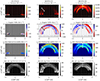 |
Fig. 5. MUSE synthetic maps, from PLUTO 3D MHD model of the multi-threaded magnetic flux tube discussed in Section 2. Here we show the tube structure at time ∼180 s after the onset of the instability and with the loop in off-limb configuration (LoS along the |

As shown in Fig. 3, the emission in the Fe IX line peaks around 1 MK. Figure 4 shows that the bulk of the flux tubes is soon heated to higher temperatures. As a consequence, the emission in this line mostly comes from the transition region at the footpoints, where the temperature steadily remains around 1 MK. On the other hand, the Fe XV line is emitted higher in the flux tubes, although the loop is still not entirely bright at this time.
For the hot Fe XIX line, we show the emission maps rebinned on macropixels (0.4″ × 2.7″), increasing the level of emission closer to the detection level (De Pontieu et al. 2020). We acknowledge that the emission in this line would come mostly from the region around the loop apex, where the temperature can reach around 10 MK.
The second row of Fig. 5 shows the Doppler shifts maps obtained as the first moment of the velocity distribution along the LoS (see Eq. (7)). For the Fe IX line, we show only the regions where the emission is within 5% of the maximum intensity, because we focus our attention on the brightest, low part of the loop. The overlapping velocity patterns along the LoS similar to those shown in Fig. 2 (bottom left) designate an irregularly alternate Doppler shift pattern at the footpoints visible in the Fe IX line, generally below 25 km s−1, complicated by the starting instability.
The Fe XV line captures the emission from most of the loop and emphasizes the chaotic filamentary (cross-section on the order of 1000 km) pattern of alternating blue-red shifts (≤50 km s−1), due to the initial MHD instability. Within the limitations above, we might infer a similar pattern (with higher speeds to about 100 km s−1) also in the Fe XIX line, although the structuring does not overlap with the Fe XV one, because of different contributions along the LoS.
The third row shows maps of the second moment of each line, which is a proxy of the non-thermal line broadening. As a reference, we mention that the thermal line broadenings as defined in Eq. (5), at the line peak temperatures, namely, T = 0.9 MK for the Fe IX line, T = 2.5 MK for the Fe XV line, and T = 10 MK for the Fe XIX line, is 16 km s−1, 27 km s−1, and 54 km s−1, respectively. The non-thermal broadening describes co-existing velocity components in different directions along the LoS. In very elongated structures, the thermal and non-thermal components are comparable; however, for the Fe XV (and Fe XIX) line in outer shells, the latter can exceed the former significantly, with a chaotic structure resembling that of the Doppler shifts. In the Fe XV line, there is a long strip around the loop apex where the non-thermal broadening exceeds 75 km s−1. The fourth row shows the maximum of the current density-magnetic field ratio (per each pixel plasma column) in three temperature bins, around the temperature peak of each line, to locate the regions where reconnection is most likely to occur.
Figure 6 shows the synthetic line profiles for the Fe IX, Fe XV, and Fe XIX lines, as a function of height z, slit number, and Doppler shift velocity, in a slit-like format, similar to the expected direct output of the spectrometer (e.g., De Pontieu et al. 2022, Fig. 4). These profiles account for both the thermal and non-thermal line broadening since they have been obtained from the integration of the single-cell Gaussian profiles (see Eq. (4)) along the LoS and the angular coverage of each slit. The Fe IX line, bright at the footpoints only, does not show significant overall Doppler shift. The Fe XV line, brighter low in the loop, shows some distortion when moving to the upper and fainter regions. In the faintest top region we also see an oscillatory trend.
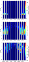 |
Fig. 6. MUSE synthetic line profiles for Fe IX, Fe XV and Fe XIX emission line, as a function of height, z, slit number, and Doppler shift velocity, as seen in Fig. 5. The spectral bins here are Δv = 25 km s−1 for Fe IX, Δv = 30 km s−1 for Fe XV, and Δv = 40 km s−1 for Fe XIX. The angular pixel along z is 0.4″, equivalent to 290 km (see Appendix A) for Fe IX and Fe XV lines and 2.7″ for Fe XIX. The positions of the profiles shown in Fig. 10 are marked (circle, diamond and star). |
Regarding the Fe XIX line, we might say (solely in generical sense) that we could expect to see some Doppler shifts that are more on the blue side, but only if we had enough sensitivity in the top loop region. In general, having multi-slit allows us to see all these features across the loop in these three lines in the same instance.
4.2. Top view
Figure 7 shows the MUSE synthetic images from a different perspective, with the LoS along  (i.e. the loop is observed from the top) at times of t = 285 s, when the emission intensity is high in all three lines. Also in this case, the maximum current density (weighted for the strength of the magnetic field) in the three lines temperature bins is shown in the fourth row, as in Fig. 5.
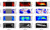 |
Fig. 7. MUSE synthetic maps at time ∼285 s and with the LoS along the |


In Fig. 7, as expected, the Fe IX line intensity map shows bright footpoints at the sides, with no emission in between. In particular, helical patterns map the footpoint rotations of the two flux tubes. The upper tube is better defined because not involved in the kink instability yet. The related Doppler map shows mostly blue shifts of up-moving plasma, driven by the heating. At the footpoints, the non-thermal broadening is noisy and mostly below 20 km s−1. Overall, it maps the current density pattern rather well.
The Fe XV line is bright along most of the loop, but more so in the lower, kink-unstable loop than in the upper kink-stable loop. Significant blue-shifts at about 100 km s−1 are present low in the loop legs, marking bulk upflows. An alternation of blue and red shifts are present high in the loop. Non-thermal broadening above 50 km s−1 is located at intermediate heights it and maps the structuring of the current density quite well.
Also, from this perspective, the hot Fe XIX line is at its brightest around the loop apex and, in particular, at the boundary between the two flux tubes (in the mid plane). The Doppler shift pattern is diluted by rebinning, except for a couple of spots of redshift and non-thermal broadening.
4.3. Time evolution
In Fig. 5, we mark the cross-sections along the loop where each line is bright and we use them to analyse the time evolution of the lines emission. In Fig. 8, we show the same quantities as in the top three rows of Fig. 5, but considering three single slits (marked in Fig. 5) as a function of time. The time of Fig. 5 (t = 180 s) is marked.
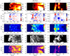 |
Fig. 8. Same as in Fig. 5, but considering the three single slits marked in Fig. 5, as a function of time and of the distance from the loop’s inner radius r. Times from Fig. 5 are shown as solid vertical lines. |
The Fe IX line, sampled at one loop footpoint, starts to brighten quite early (t ∼ 100 s) overall and, in particular, in correspondence to the outer shell of the loop. While it does not occur uniformly, the brightness increases progressively over time. Conversely, the Doppler shift and the non-thermal broadening show higher values earlier in the evolution, around 150–200 s. Both of them have a patchy pattern, with alternating red and blue Doppler shifts and high small-line broadening, respectively.
The Fe XV line brightens significantly after t = 200 s, which is quite later than the Fe IX line, because of the time taken by dense plasma to come up from the chromosphere. The brightening is more uniform than that seen for the Fe IX line and it already gets to its peak, in part of the loop, at about t = 300 s. Also in this case we have more significant dynamics at early times (between t = 100 s and t = 300 s), with Doppler shifts declining well below 50 km s−1 and broadenings below 20 km s−1 by the time the intensity peak is reached. However, the predicted intensities are already high enough (De Pontieu et al. 2020) at the time of peak shift or broadening to detect those line properties. In the Doppler-shift maps, we see more defined alternating red and blue patterns both in terms of the time and along the slit.
While it is quite faint, the Fe XIX line, emitted at the loop top, brightens very early (t ∼ 100 s), for a short time and with an irregular pattern, marking the time interval when the heating from reconnection is most effective (because the density is still relatively low) and the temperature has a peak (see Fig. 9 in Cozzo et al. 2023b). In the interval between 100 s and 300 s we also see a bright spot of blue shift (100 km s−1) and one of line broadening (100 km s−1.)
Figure 9 is similar to Fig. 8, but the evolution is taken along a line in the XY plane, with a LoS that is parallel to the Z-direction (top view). Also, in this case, we see an increasing line luminosity in the Fe IX and Fe XV lines and flashes in the Fe XIX line. The evolution of the Doppler shifts cut shows clearly the presence of strong and long-lasting upflows from the loop footpoints (Fe IX).
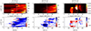 |
Fig. 9. Same details as in the top two rows of Fig. 7, but considering three single slits (slit numbers 2, 4, and 6 in Fig. 7, for the Fe IX, Fe XV, and Fe XIX lines, respectively), as a function of time and y. The time of Fig. 7 is marked (solid vertical lines). |
Movie 1 shows the system evolution in the side view of Fig. 5, from the onset of the instability to 500 s, when the system is close to a steady state. Significant currents appear first in the low temperature bin and around the loop apex at the onset of the instability and then again after 1 min in the other temperature bins. After about 2 min, when the plasma suddenly reaches 10 MK, we see some faint emission at the top in the Fe XIX line, which rapidly extends down along the loop. At about t = 150 s we start to see emission also in the other two lines, starting from the loop footpoints, and then propagating upwards in the Fe XV line only. At t = 300 s the whole loop appears illuminated in this line, while the Fe XIX line rapidly disappears completely. In the Fe XV line, we clearly see bright fronts moving up and down and also that the brightness is not uniform across the loop, but with a filamented structuring which changes in time.
The Doppler shift images have quite well defined patterns around t = 170 s (blue on the right, red on the left in the Fe XV line), alternating wide strips in the Fe XIX line. These patterns rapidly become finely structured and chaotic by t ∼ 200 s in both lines. In the first 2 min, we also see large intense (red) spots of non-thermal broadening in the same two lines, which become filamentary later on, until they decrease significantly below 50 km s−1 after about 5 min. The movie confirms that there is some level of correspondence between the evolution and structuring of the non-thermal broadening in the Fe XV line and those of the current density.
When looking more closely at the single lines, the Fe XIX line shows a brightening strip at the onset of the first instability (130 s < t < 160 s) at the low boundary around the apex of the curved tube. There we can also see some blue-shift, more to the left, a spot of non-thermal broadening (> 100 km/s) and intense current density. These features are produced by the folding of elongated structures which align along the LoS. We see an analogous effect at the onset of the second instability (250 s < t < 290 s), this time involving more the top boundary. The evolution of the Fe XV line emission is more independent of the onset of the instabilities. In this side view, the loop starts to brighten from the footpoints after t = 150 s and is filled in about 100 s. Then, its intensity increases more or less uniformly and progressively. Irregular Doppler-shifts and non-thermal broadening patterns are more intense at some times but progressively fade out. The Fe IX line shows irregular patterns, which are difficult to discern as they are very flat at the footpoints.
Movie 2 shows the system evolution (analogously to Movie 1) from the top view of Fig. 7. Again we clearly see the first brightening in the Fe XIX line in a thin strip at the boundary between the two rotating tubes (t = 125 s). Then the first unstable loop brightens up in all lines at the same time. At t = 153 s, bright helices appear at the footpoints in both Fe XV and Fe IX lines and a broad oblique band extending over the whole loop length in the Fe XIX line. The Fe XV and Fe IX brightenings rapidly extent to the other flux tube, with two definite helices. The helices rapidly blur and fade away in the Fe XV line, while the emission gradually bridges over the whole loop region. Initially, it is brighter in the first unstable tube. In the Fe XIX line, there are rapid faint flashes of few tens of seconds involving different, but relatively large coronal regions: the first unstable tube earlier and the other one later. Regarding the Doppler shifts, this view clearly shows the expected strong upflows as the flux tubes initiate the instability, from t ∼ 200 s. We see strong blueshifts in the first unstable tube at the footpoints in the Fe IX line, propagating to the body of the loop in the Fe XV line, and continuing with redshifts in the Fe XIX line flows, moving from one side to the other.
Also, from this view, we see the strongest non-thermal broadenings soon after the instabilities are triggered in both flux tubes, with a structuring similar to the one shown by the current density, especially in the Fe XV and Fe XIX lines. In particular, the Fe XIX line confirms the large non-thermal broadening when the line is more intense. Looking in more detail at each line, in the Fe XIX line emission boundary strips brighten again, due to the folding of emission sheets that overlap along the LoS. At the same time, there are significant downflows and line broadening, downstream, or close to the areas of intense current density.
The Fe IX emission shows the helical patterns clearly at the onset of the instability (t > 150 s, t > 260 s). Alternating blueshifts and redshifts are also present at the onset of the instability (t = 167 s, with velocity v > 50 km/s), then blue-shifts become dominant (t > 200 s). Transient non-thermal broadenings are present for 160s < t < 330 s (3 min, Δv ∼ 30 km/s).
In the Fe XV line, we see the ignition of the lower part of the first unstable tube at t = 167 s, the whole tube is bright at t = 264 s. The other tube starts to brighten at t = 264 s, and is entirely bright at t = 313 s. Strong blueshifts appear at the footpoints early after each tube becomes unstable and extends upwards. Redshifts are present in area of weak emission, as well as large non-thermal broadenings.
5. Discussion and conclusions
This work addresses how coronal loops, heated by an MHD avalanche process, would be observed with the forthcoming MUSE mission. It is an extension of the modeling-oriented work described in Cozzo et al. (2023b) and it delves into the synthesis of spectroscopic observations in Fe IX, Fe XV, and Fe XIX lines with the forthcoming MUSE mission, which will probe plasma at ∼1 MK, ∼2 MK, and ∼10 MK, respectively, at high spatial and temporal resolution.
In this work, forward-modeling bridges theoretical investigation of loop heating through MHD instability (Hood et al. 2009; Cozzo et al. 2023b) with realistic observations in the EUV band. This approach represents a significant progress both because it is based on a non-ideal MHD model (see also Guarrasi et al. 2014; Cozzo et al. 2023a) and because it realistically accounts for future instrumental improvements (the MUSE mission). In particular, we provide specific observational constraints that are useful for testing the model and guide future modeling efforts. Forward-modeling for comparison with real observations requires a very detailed and complete physical description and including the space-time dependence at different spectral lines makes this task even more difficult. Historically, time-dependence has been possible using the 1D hydrodynamic modeling applied, for instance, to the light curves and line spectra of impulsively heated loops, (e.g., Peres et al. 1987; Antonucci et al. 1993; Testa et al. 2014). Constraints on the heating parameters of non-flaring loops were derived from comparing space-time dependent loop modeling with the brightness distribution and evolution observed with TRACE (Reale et al. 2000a,b) and SDO/AIA (Price et al. 2015). Collections of single loop models have been used to synthesize the emission and patterns of entire active regions (Warren & Winebarger 2007; Bradshaw & Viall 2016). Collections of 1D loop models have been used also to describe the emission of multi-stranded loops (Guarrasi et al. 2010).
Regarding proper multi-D MHD loop modeling, Reale et al. (2016) showed the synthetic emission of a coronal loop heated by twisting in two EUV (SDO/AIA 171 Å and 335 Å, Lemen et al. 2012; Pesnell et al. 2012) channels and in one X-ray (Hinode/XRT Ti-poly, Lee et al. 2009) channel. Also in that case, only the transition region footpoints brighten in the 171 Å channel since the loop plasma is mostly at temperatures around 2⌣3 MK, at which the 335 Å channel is more sensitive. The central region of the coronal loop, at higher temperature plasma, is also bright in the X-ray band.
A list of preliminary applications of MHD forward-modeling to the MUSE mission is reported in De Pontieu et al. (2022) and Cheung et al. (2022). They show that Doppler shifts and line broadening are important tools to provide key diagnostics of the mechanisms behind coronal activity. Moreover, they point out the importance of coupling high-cadence, high-resolution observations with advanced numerical simulations.
The full 3D MHD model in Cozzo et al. (2023b) describes a release of magnetic energy in a stratified atmosphere. It accounts for a multi-threaded coronal loop made up by two (or more) interacting magnetic strands, subjected to twisting at the photospheric boundaries. The global, turbulent decay of the magnetic structure is triggered by the disruption of a single coronal loop strand, made kink-unstable by twisting. Massive reconnection episodes are triggered and determine local impulsive heating and rapid rises in temperature. These are then tempered by efficient thermal conduction and optically-thin radiative losses. The overpressure drives the well-known chromosphere evaporation into the hot corona and consequent loop brightening in the EUV and X-ray bands.
The model allows for both space and time resolved diagnostics. In particular, we synthesized MUSE observations in the Fe IX, Fe XV, and Fe XIX emission lines, sensitive to a wide range of emitting plasma temperature, i.e., ∼1 MK, ∼2 MK, and ∼10 MK, respectively.
The modeled loop is a typical active region loop of length 50 Mm with an average temperature of about 2.5 MK. As such, much of it its brightness is steadily in the Fe XV line, only at the footpoints in the Fe IX line, and (very faintly and transiently) at the apex of the Fe XIX line.
The loop is initially cold (T ≲ 1 MK) and tenuous (n ∼ 108 cm−3), with faint emission only in the 171 Å channel of Fe IX. Rapid, high temperature peaks, with faint emission in the Fe XIX line, occur during the dynamic phase of the instability, but most of the radiation is emitted by Fe XV at a temperature of ≳2 MK (Fig. 4).
In Fig. 6, we show the overall distribution of lines intensity and shape at time ∼180 s. In this case, line profiles show deviations from the Gaussian profile, such as an asymmetric shape and/or multiple peaks, as a consequence of the dynamic and impulsive behaviour of the instability. This is remarked also in Fig. 10 with three examples of Fe IX (solid), Fe XV (dashed), and Fe XIX (dotted) profiles at different slits and heights. The main peak of the Fe IX line is almost at rest, whereas Fe XV and Fe XIX show strong Doppler shifts (blue and red, respectively, at |v|≳50 km s−1). In all these cases, there is an increase of non-thermal width in locations where reconnection seems to occur. In particular, multi Gaussian components appear in Fe IX line (small, red-shifted peak at v ∼ 100 km s−1), in the Fe XIX line (small, blue-shifted peak at v ∼ −100 km s−1) and the Fe XV line (strong contribution at rest).
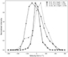 |
Fig. 10. Detailed (normalized) profiles of the Fe IX (solid), Fe XV (dashed), and Fe XIX (dotted) lines at the positions marked in Fig. 6. |
Testa & Reale (2020) show evidence of plasma heated at 10 MK during a microflare. In particular, they analyzed the coronal (131 and 94 Å channels of AIA) and spectral (Fe XXIII 263.76 Å line of Hinode/EIS) imaging and compared observations with hydrodynamic 1D modeling of a single loop heated by a 3 min pulse up to 12 MK. Forward modeling from the simulations provides additional evidence of the coronal loop multistructuring into independently heated substrands.
We have obtained results in both a spatially resolved (Section 4.1) and a time-resolved (Section 4.3) fashion. In all cases, we conclusively show how the three lines provide plasma information at different places, dynamical stages, and physical conditions. In particular, we have managed to efficiently disentangle the instability evolution into: (Fe IX) foot point response and plasma ablation in the transition region; (Fe XV) over-dense and warm plasma rising at intermediate heights; and, faintly in this case, (Fe XIX) hot flaring plasma inside current sheets.
Progressive brightening is expected in the cooler lines, while we expect that the hottest line might be bright only occasionally and with a lower count rate. This is due to the low densities at the loop apex and the small filling factor, namely, only a small plasma volume gets close to the Fe XIX line formation temperature. We might expect more emission for higher temperature loops, as produced, for instance, by a stronger background magnetic field. The hot Fe XIX shows faint emission here as soon as the flux tube becomes unstable, therefore, it may potentially become a signature of the initial phase of the instability. Fe XIX emission is expected to be short-lived and around the loop top, to be compared with recent evidence of traces of very hot plasma (e.g., Ishikawa et al. 2017; Miceli et al. 2012).
In this analysis, we have reproduced expected line profiles integrated along possible lines of sight (Fig. 6). In a limb snapshot view (Fig. 5), MUSE observations might show alternating red-blue patterns along the loop, especially in the Fe XV line. The non-thermal broadening might be also quite irregular with filamented structure. The line profiles taken in a side view might show an irregular trend across the loop in the hot lines. The top view (Fig. 7) provides complementary information, helical patterns in the footpoints region, and systematic blue-shifts in the loop legs during the rise phase, but also possible faint one-way flows and filamented non-thermal patterns in the corona. More intense plasma dynamics from Doppler-shifts and non-thermal broadenings are expected during loop ignition, namely, just after the onset on the instabilities and avalanche process. Blue-shifts might be more persistent in the 1 MK line. Cross-structuring is ultimately linked to the assumptions on dissipation, in particular the resistivity determines the cross-size. The photospheric drive plays a role too close to the strands footpoints while it does not seem to influence cross-structuring in the upper corona. MUSE observations might provide crucial information. The instability propagates with a delay of about 2 min, the timing depends on some assumptions (thickness of the flux tubes/rotation radius, rotation rate, field intensity).
The Fe XIX line (if detectable) might be a fair proxy of strong and dynamic current buildups such as current sheets. They form and rapidly dissipate during the earliest, most violent phase of the instability. At the same time (i.e., at the time of the disruption of the threads), the Fe IX footpoint emission provides complementary information about the status of the magnetic structure (Fig. 2), suggesting a potential diagnostics role in terms of extrapolating information about the linear phase of the instability (Fig. 7), as it might outclass the observational restriction imposed by the small counts-rate obtained with Fe XIX line (De Pontieu et al. 2020).
After the early stages of the instability, Fe XV emission returns information about the evaporation process triggered by the avalanche. This is the only case in which almost the whole coronal loop structure becomes visible to the instrument.
Doppler shifts and non-thermal line broadening can provide additional information about the plasma dynamics, confirming the strongly turbulent behaviour of the avalanche process, which is otherwise difficult to grasp only from emission maps analysis. Doppler-shift maps also contribute complementary information on the strength of the chromospheric evaporation nearby footpoints (Fig. 7). Indeed, after the instability, the lines from the simulation broaden and strongly blue-shift, due to the strong chromospheric evaporation up-flows and in agreement also with Testa & Reale (2020) forward modeling of 1D microflaring coronal loop.
According to the estimated uncertainties in centroid and line width determination discussed in De Pontieu et al. (2020), minimum line intensities of ∼100/150 photons for Fe IX/Fe XV, lines and ∼20 photons for Fe XIX, are required to obtain the desired accuracy. In our simulations, Fe IX, and Fe XV, Doppler shifts, and non-thermal line broadening can be accurately estimated in the brightest regions (above 5% of the intensity peak) and with exposure times of ≳5 s. Emission in the Fe XIX MUSE line would perhaps be detectable only with particularly deep exposures (> 30 s) with our setup, but with shorter exposures for stronger magnetic field.
This work addresses in detail the observability of a 2 MK coronal loop system that is triggered by an MHD instability and described by a full 3D MHD model. To be specific, this forward-modeling approach is applied to the EUV spectrometry to be obtained with the forthcoming MUSE mission. Although calibrated on the high capabilities of this ambitious mission, our analysis is generally valid for observations made with instruments working in similar bands, such as present-day SDO/AIA, Hinode/EIS, Solar Orbiter SPICE (Anderson et al. 2020), and EUI (Rochus et al. 2020), or the forthcoming Solar-C/EUVST as well. The capabilities in terms of spatial, temporal, and spectral resolution of current observations (e.g., SDO/AIA, Hinode/EIS, Solar Orbiter SPICE and EUI) do not allow us to reach the diagnostic level shown by our analysis and further support the implementation of the MUSE mission.
Data availability
Movies are available at https://www.aanda.org
Acknowledgments
GC, PP, and FR acknowledge support from ASI/INAF agreement n. 2022-29-HH.0. This work made use of the HPC system MEUSA, part of the Sistema Computazionale per l’Astrofisica Numerica (SCAN) of INAF-Osservatorio Astronomico di Palermo. JR and AWH acknowledge the financial support of Science and Technology Facilities Council through Consolidated Grant ST/W001195/1 to the University of St Andrews. PT was supported by contract 4105785828 (MUSE) to the Smithsonian Astrophysical Observatory, and by NASA grant 80NSSC20K1272x.
References
- Alfvén, H. 1947, MNRAS, 107, 211 [CrossRef] [Google Scholar]
- Anderson, M., Appourchaux, T., Auchère, F., et al. 2020, A&A, 642, A14 [NASA ADS] [CrossRef] [EDP Sciences] [Google Scholar]
- Antonucci, E., Dodero, M., Martin, R., et al. 1993, ApJ, 413, 786 [CrossRef] [Google Scholar]
- Boerner, P., Edwards, C., Lemen, J., et al. 2012, Sol. Dyn. Obs., 41 [Google Scholar]
- Bradshaw, S. J., & Viall, N. M. 2016, ApJ, 821, 63 [NASA ADS] [CrossRef] [Google Scholar]
- Cheung, M. C., Martínez-Sykora, J., Testa, P., et al. 2022, ApJ, 926, 53 [NASA ADS] [CrossRef] [Google Scholar]
- Cirtain, J. W., Golub, L., Winebarger, A., et al. 2013, Nature, 493, 501 [NASA ADS] [CrossRef] [Google Scholar]
- Cozzo, G., Pagano, P., Petralia, A., & Reale, F. 2023a, Symmetry, 15, 627 [NASA ADS] [CrossRef] [Google Scholar]
- Cozzo, G., Reid, J., Pagano, P., Reale, F., & Hood, A. W. 2023b, A&A, 678, A40 [NASA ADS] [CrossRef] [EDP Sciences] [Google Scholar]
- Culhane, J. L., Harra, L. K., James, A. M., et al. 2007, Sol. Phys., 243, 19 [Google Scholar]
- De Pontieu, B., Martínez-Sykora, J., Testa, P., et al. 2020, ApJ, 888, 3 [NASA ADS] [CrossRef] [Google Scholar]
- De Pontieu, B., Testa, P., Martínez-Sykora, J., et al. 2022, ApJ, 926, 52 [NASA ADS] [CrossRef] [Google Scholar]
- Del Zanna, G., Dere, K., Young, P., & Landi, E. 2021, ApJ, 909, 38 [NASA ADS] [CrossRef] [Google Scholar]
- Edlén, B. 1943, Zeitschrift für Astrophysik, 22, 30 [Google Scholar]
- Feldman, U. 1992, Phys. Scr., 46, 202 [CrossRef] [Google Scholar]
- Grotrian, W. 1939, Naturwissenschaften, 27, 555 [NASA ADS] [CrossRef] [Google Scholar]
- Guarrasi, M., Reale, F., & Peres, G. 2010, ApJ, 719, 576 [NASA ADS] [CrossRef] [Google Scholar]
- Guarrasi, M., Reale, F., Orlando, S., Mignone, A., & Klimchuk, J. 2014, A&A, 564, A48 [NASA ADS] [CrossRef] [EDP Sciences] [Google Scholar]
- Hood, A. W., & Priest, E. 1979, Sol. Phys., 64, 303 [NASA ADS] [CrossRef] [Google Scholar]
- Hood, A., Browning, P., & Van der Linden, R. 2009, A&A, 506, 913 [NASA ADS] [CrossRef] [EDP Sciences] [Google Scholar]
- Hood, A. W., Cargill, P., Browning, P., & Tam, K. 2016, ApJ, 817, 5 [NASA ADS] [CrossRef] [Google Scholar]
- Ishikawa, S.-N., Glesener, L., Krucker, S., et al. 2017, Nat. Astron., 1, 771 [NASA ADS] [CrossRef] [Google Scholar]
- Klimchuk, J. A. 2009, ArXiv e-prints [arXiv:0904.1391] [Google Scholar]
- Klimchuk, J. A. 2015, Philos. Trans. R. Soc. A: Math. Phys. Eng. Sci., 373, 20140256 [NASA ADS] [CrossRef] [Google Scholar]
- Lee, J.-Y., Leka, K., Barnes, G., et al. 2009, ASP Conf. Ser., 415, 279 [NASA ADS] [Google Scholar]
- Lemen, J. R., Title, A. M., Akin, D. J., et al. 2012, Sol. Phys., 275, 17 [Google Scholar]
- Linker, J. A., Lionello, R., Mikic, Z., & Amari, T. 2001, J. Geophys. Res., 106, 25165 [NASA ADS] [CrossRef] [Google Scholar]
- Lionello, R., Linker, J. A., & Mikic, Z. 2009, ApJ, 690, 902 [CrossRef] [Google Scholar]
- Miceli, M., Reale, F., Gburek, S., et al. 2012, A&A, 544, A139 [NASA ADS] [CrossRef] [EDP Sciences] [Google Scholar]
- Mignone, A., Bodo, G., Massaglia, S., et al. 2007, ApJS, 170, 228 [Google Scholar]
- Mikic, Z., Lionello, R., Mok, Y., Linker, J. A., & Winebarger, A. R. 2013, ApJ, 773, 112 [NASA ADS] [CrossRef] [Google Scholar]
- Parker, E. N. 1988, ApJ, 330, 474 [Google Scholar]
- Parnell, C. E., & De Moortel, I. 2012, Philos. Trans. R. Soc. A: Math. Phys. Eng. Sci., 370, 3217 [NASA ADS] [CrossRef] [Google Scholar]
- Peres, G., Reale, F., Serio, S., & Pallavicini, R. 1987, ApJ, 312, 895 [NASA ADS] [CrossRef] [Google Scholar]
- Pesnell, W. D., Thompson, B. J., & Chamberlin, P. 2012, The Solar Dynamics Observatory (SDO) (Springer) [Google Scholar]
- Peter, H., & Dwivedi, B. N. 2014, Front. Astron. Space Sci., 1, 2 [NASA ADS] [CrossRef] [Google Scholar]
- Price, D. J., Taroyan, Y., Innes, D., & Bradshaw, S. J. 2015, Sol. Phys., 290, 1931 [NASA ADS] [CrossRef] [Google Scholar]
- Reale, F. 2014, Liv. Rev. Sol. Phys., 11, 1 [NASA ADS] [Google Scholar]
- Reale, F., Peres, G., Serio, S., et al. 2000a, ApJ, 535, 423 [NASA ADS] [CrossRef] [Google Scholar]
- Reale, F., Peres, G., Serio, S., DeLuca, E., & Golub, L. 2000b, ApJ, 535, 412 [NASA ADS] [CrossRef] [Google Scholar]
- Reale, F., Orlando, S., Guarrasi, M., et al. 2016, ApJ, 830, 21 [CrossRef] [Google Scholar]
- Reid, J., Hood, A. W., Parnell, C. E., Browning, P., & Cargill, P. 2018, A&A, 615, A84 [NASA ADS] [CrossRef] [EDP Sciences] [Google Scholar]
- Reid, J., Cargill, P., Hood, A. W., Parnell, C. E., & Arber, T. D. 2020, A&A, 633, A158 [NASA ADS] [CrossRef] [EDP Sciences] [Google Scholar]
- Rochus, P., Auchere, F., Berghmans, D., et al. 2020, A&A, 642, A8 [NASA ADS] [CrossRef] [EDP Sciences] [Google Scholar]
- Shimizu, T., Imada, S., Kawate, T., et al. 2019, in UV, X-Ray, and Gamma-Ray Space Instrumentation for Astronomy XXI (SPIE), 11118, 27 [Google Scholar]
- Tam, K. V., Hood, A. W., Browning, P., & Cargill, P. 2015, A&A, 580, A122 [NASA ADS] [CrossRef] [EDP Sciences] [Google Scholar]
- Testa, P., & Reale, F. 2020, ApJ, 902, 31 [NASA ADS] [CrossRef] [Google Scholar]
- Testa, P., & Reale, F. 2023, in Handbook of X-ray and Gamma-ray Astrophysics, eds. C. Bambi, & A. Santangelo, 134 [Google Scholar]
- Testa, P., De Pontieu, B., Allred, J., et al. 2014, Science, 346, 1255724 [Google Scholar]
- Tsuneta, S., Ichimoto, K., Katsukawa, Y., et al. 2008, Sol. Phys., 249, 167 [Google Scholar]
- Vaiana, G., Krieger, A., & Timothy, A. 1973, Sol. Phys., 32, 81 [NASA ADS] [CrossRef] [Google Scholar]
- Warren, H. P., & Winebarger, A. R. 2007, ApJ, 666, 1245 [NASA ADS] [CrossRef] [Google Scholar]
- Zirker, J. B. 1993, Sol. Phys., 148, 43 [NASA ADS] [CrossRef] [Google Scholar]
Appendix A: Data interpolation
To resemble the typical, semicircular, coronal loops shape, the original simulation results have been remapped and interpolated onto a new cartesian grid (see Fig. A.1). In particular, points (x, y, z) in the original grid corresponds to points  defined by equations (A.1) for the corona and (A.2) for the chromospheric layer.
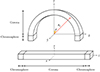 |
Fig. A.1. Original and interpolated box geometry. Lower picture: schematic representation of the 3D box containing the computational domain of the simulation. Upper picture: geometry of the interpolated domain mapping the straight flux tube into a curved one. |
Specifically, the coronal region of the domain (z ∈ [−L,L]) is transformed into a half cylinder shell with characteristic radius R0 = 2 L/π:
![Mathematical equation: $$ \begin{aligned} {\left\{ \begin{array}{ll} \tilde{x} = R \sin \theta , \\ \tilde{y} = x, \\ \tilde{z} = R \cos \theta . \end{array}\right.} \mathrm{ for } z \in \left[-L, L\right] \end{aligned} $$](/articles/aa/full_html/2024/09/aa50644-24/aa50644-24-eq18.gif) (A.1)
(A.1)
with R = R0 + y and  .
.
The chromospheric layers are instead threaded as two parallel parallelepipeds of height zmax − L:
 (A.2)
(A.2)
New vectors components  , such as velocity and magnetic field, are obtained from the former (vx, vy, vz) using the following rule:
 (A.3)
(A.3)
where both triads  and vi are functions of
  . In general, the correspondence between the former set of coordinates and latter is that the gravity vector g points uniformly along
  . Magnetohydrodynamic quantities are interpolated and rebinned in the new geometry at the given instrument resolution. In particular the grid pixel size, i.e. the dimension of the cells edges perpendicular to the LoS, will be equal to 170 km × 290 km, corresponding to 0.16″ × 0.4″ i.e. the angular extension of the instrument’s pixel (parallel and perpendicular to the slits orientation).
Figure 4 shows the resulting field line configuration colored by temperature in the new geometry at the three times already shown in Fig. 1.
All Tables
All Figures
|
Fig. 1. 3D rendering of the magnetic field lines inside the box at times (from left to right): t = 0 s (initial condition), 180 s, (first loop disruption), and 500 s. The change in the field line connectivity during the evolution of the MHD cascade is emphasized by the colors. |
| In the text | |
|
Fig. 2. MHD avalanche 2D snapshots. Upper panels. Horizontal cuts of the current density across the mid plane at time t = 180 s (left) and t = 285 s (right). The green contours encloses the regions of the domain heated by ohmic dissipation. Lower panels. Horizontal cuts of the magnetic field across the mid-plane at the same snapshot-times as before. The vector field is included. |
| In the text | |
|
Fig. 3. Response function Λi(T) for the three MUSE emission lines (Fe IX, Fe XV, and Fe XIX) as a function of temperature. |
| In the text | |
|
Fig. 4. 3D rendering of the magnetic field lines inside the box at the same times shown in Fig. 1. Magnetic field lines are color-coded according to the plasma temperature. |
| In the text | |
|
Fig. 5. MUSE synthetic maps, from PLUTO 3D MHD model of the multi-threaded magnetic flux tube discussed in Section 2. Here we show the tube structure at time ∼180 s after the onset of the instability and with the loop in off-limb configuration (LoS along the |
| In the text | |
|
Fig. 6. MUSE synthetic line profiles for Fe IX, Fe XV and Fe XIX emission line, as a function of height, z, slit number, and Doppler shift velocity, as seen in Fig. 5. The spectral bins here are Δv = 25 km s−1 for Fe IX, Δv = 30 km s−1 for Fe XV, and Δv = 40 km s−1 for Fe XIX. The angular pixel along z is 0.4″, equivalent to 290 km (see Appendix A) for Fe IX and Fe XV lines and 2.7″ for Fe XIX. The positions of the profiles shown in Fig. 10 are marked (circle, diamond and star). |
| In the text | |
|
Fig. 7. MUSE synthetic maps at time ∼285 s and with the LoS along the |
| In the text | |
|
Fig. 8. Same as in Fig. 5, but considering the three single slits marked in Fig. 5, as a function of time and of the distance from the loop’s inner radius r. Times from Fig. 5 are shown as solid vertical lines. |
| In the text | |
|
Fig. 9. Same details as in the top two rows of Fig. 7, but considering three single slits (slit numbers 2, 4, and 6 in Fig. 7, for the Fe IX, Fe XV, and Fe XIX lines, respectively), as a function of time and y. The time of Fig. 7 is marked (solid vertical lines). |
| In the text | |
|
Fig. 10. Detailed (normalized) profiles of the Fe IX (solid), Fe XV (dashed), and Fe XIX (dotted) lines at the positions marked in Fig. 6. |
| In the text | |
|
Fig. A.1. Original and interpolated box geometry. Lower picture: schematic representation of the 3D box containing the computational domain of the simulation. Upper picture: geometry of the interpolated domain mapping the straight flux tube into a curved one. |
| In the text | |
Current usage metrics show cumulative count of Article Views (full-text article views including HTML views, PDF and ePub downloads, according to the available data) and Abstracts Views on Vision4Press platform.
Data correspond to usage on the plateform after 2015. The current usage metrics is available 48-96 hours after online publication and is updated daily on week days.
Initial download of the metrics may take a while.