| Issue |
A&A
Volume 681, January 2024
|
|
|---|---|---|
| Article Number | L11 | |
| Number of page(s) | 7 | |
| Section | Letters to the Editor | |
| DOI | https://doi.org/10.1051/0004-6361/202347790 | |
| Published online | 11 January 2024 | |
Letter to the Editor
Identifying Alfvén wave modes in the solar corona
1
School of Mathematics and Statistics, University of St Andrews, St Andrews, Fife KY16 9SS, UK
e-mail: ee30@st-andrews.ac.uk
2
Rosseland Centre for Solar Physics, University of Oslo, PO Box 1029 Blindern, 0315 Oslo, Norway
3
School of Design and Informatics, Abertay University, Bell Street, Dundee DD1 1HG, UK
Received:
23
August
2023
Accepted:
6
November
2023
Context. Oscillations are observed to be pervasive throughout the solar corona, but it remains challenging to positively identify different wave modes. Improving this identification would provide a powerful tool for investigating coronal wave heating and improving seismological inversions.
Aims. We aim to establish whether theoretical methods used to identify magnetohydrodynamical wave modes in numerical simulations can be employed on observational datasets.
Methods. We applied wave identifiers based on fundamental wave characteristics such as compressibility and direction of propagation to a fully 3D numerical simulation of a transversely oscillating coronal loop. The same wave identifiers were applied to the line-of-sight integrated synthetic emission derived from the numerical simulation data to investigate whether this method could feasibly be useful for observational studies.
Results. We established that for particular line(s) of sight and assumptions about the magnetic field, we can correctly identify the properties of the Alfvén mode in synthetic observations of a transversely oscillating loop. Under suitable conditions, there is a strong agreement between the simulation and synthetic emission results.
Conclusions. For the first time, we have provided a proof of concept that this theoretically derived classification of magnetohydrodynamic wave modes can be applied to observational data.
Key words: magnetohydrodynamics (MHD) / waves / instrumentation: spectrographs / Sun: corona / Sun: oscillations
© The Authors 2024
 Open Access article, published by EDP Sciences, under the terms of the Creative Commons Attribution License (https://creativecommons.org/licenses/by/4.0), which permits unrestricted use, distribution, and reproduction in any medium, provided the original work is properly cited.
This article is published in open access under the Subscribe to Open model. Subscribe to A&A to support open access publication.
1. Introduction
Although it has long been known that the solar corona is orders of magnitude hotter than the photosphere, the full details of coronal heating remain unresolved. The proposed heating mechanisms are often divided into AC and DC heating, depending on the timescales at which energy is transported. DC heating corresponds to timescales longer than the Alfvén travel time and is typically associated with magnetic reconnection (e.g. see review by Wilmot-Smith 2015). AC (or wave) heating, on the other hand, is associated with timescales shorter than the Alfvén travel time. In this paradigm, photospheric convective motions excite waves that propagate upwards through the atmosphere before dissipating their energy as heat. Despite extensive research, it remains unclear whether magnetohydrodynamic (MHD) waves contribute significantly to coronal heating (see e.g. Parnell & De Moortel 2012; Arregui 2015; Van Doorsselaere et al. 2020; Banerjee et al. 2021; Howson 2022).
In a uniform plasma, there are three distinct MHD wave modes: Alfvén, and slow and fast magnetoacoustic waves. In a non-uniform fully 3D plasma (e.g. the corona), wave modes often have mixed characteristics (e.g. Nakariakov & Verwichte 2005), and it is not trivial to correctly identify wave modes. Different wave modes are associated with different phase speeds, energy fluxes, damping mechanisms, and dissipation rates. The difficulties associated with correctly identifying these oscillations, alongside observational uncertainties, ensure that measurements of coronal wave energy flux remain poorly constrained. For example, Tomczyk et al. (2007) inferred an energy flux from Doppler perturbations (interpreted as Alfvénic waves) of 0.01 W m−2. On the other hand, McIntosh et al. (2011) estimated a value of 100 W m−2 from AIA observations, a flux that is sufficient to heat the quiet Sun and accelerate the solar wind. For further discussion, we refer to the review by Van Doorsselaere et al. (2020).
Many solar atmospheric wave models assume a simplified setup that could lead to an overestimate of the energy flux (Goossens et al. 2013). Identifying which wave modes that are observed in complex systems could therefore lead to more accurate energy flux estimates, which would improve our understanding of the role waves play in coronal heating. Furthermore, this would also have powerful implications for coronal seismology, where the observed oscillation parameters are used to deduce plasma properties such as the magnetic field strength, the density, and the temperature (e.g. Nakariakov & Kolotkov 2020; Srivastava et al. 2021).
Previously, several authors have classified MHD waves in complex media using a variety of approaches, such as velocity decomposition (Khomenko & Cally 2011, 2012; Leenaarts et al. 2015; Shelyag et al. 2016; Yadav et al. 2022). However, it is not straightforward to associate each component with one wave mode. Instead, this study uses identifiers based on fundamental wave mode characteristics such as compressibility and the direction of propagation (see also Raboonik 2022). By considering a numerical simulation of a transversely oscillating loop (De Moortel & Howson 2022), we investigate how robustly the wave identifiers track the oscillatory dynamics. By using synthetic emission derived from the simulations, we then establish how the identifiers could be used to extract information from coronal observations.
This Letter is structured as follows: In Sect. 2 we outline our method, and we also define the wave identifiers and provide context for the numerical data and the synthetic emission. In Sect. 3 we show the result of using the wave identifiers on the numerical data and synthetic emission, and in Sect. 4 we discuss our findings.
2. Method
2.1. Wave identifiers
In a uniform plasma, Alfvén waves are incompressible transverse perturbations that propagate along the magnetic field. Fast and slow magnetoacoustic waves are compressible waves. For a low-β plasma (e.g. the corona), slow waves are longitudinal sound-like waves predominantly travelling parallel to the magnetic field. Fast waves, on the other hand, propagate fastest across the magnetic field. These properties are represented in the three wave identifiers used in this study (see Raboonik 2022; for a detailed derivation):
where e∥ = B/B is the unit vector parallel to the magnetic field, B, v is the velocity, and v∥ is the velocity component parallel to the field. These identifiers provide an incompressible parallel component (νA), a compressible parallel component (ν∥), and a compressible perpendicular component (ν⊥). Although these identifiers do not coincide with the rigorous definitions of the three basic MHD wave modes, they are associated with important distinguishing characteristics of the different modes. For brevity, we refer to them as the Alfvén (νA) and the fast (ν⊥) and slow (ν∥) identifiers.
2.2. Numerical model
To demonstrate the potential of these identifiers, we used a numerical simulation first presented by De Moortel & Howson (2022). The authors modelled a coronal loop as a 3D flux tube where the magnetic field is aligned with the z-axis. The initial density has a smooth transverse profile, with the external and internal density being ρe = 1.67 × 10⁻¹³ kg m−3 and ρi = 3ρe, respectively (see Fig. 1). The initial temperature was 1 MK everywhere. At the lower z-boundary, a transverse wave driver was imposed with an amplitude of approximately 8 km s−1 and a frequency set to the natural kink frequency of the loop (see e.g. Edwin & Roberts 1983; Nakariakov & Verwichte 2005). Further details of the numerical model are presented in Appendix A. As time progresses, the smooth density profile allows for resonant absorption (or mode coupling; Ionson 1978), resulting in the transfer of wave energy from the global transverse mode to small-scale azimuthal Alfvén waves confined to the loop boundary, where they are subject to phase-mixing and the Kelvin-Helmholtz instability (KHI; see e.g. Howson 2022 for a summary of this process). We aim to track the transfer of energy between these different wave modes using the wave identifiers.
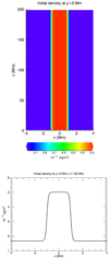 |
Fig. 1. Vertical cut (top) and horizontal cross section (bottom) of the initial density (i.e. at t = 0 s) both at y = 0 Mm. |
Figure 2 shows time-distance plots of the density and temperature at the loop apex. The density plot shows that the loop boundary broadens over time as a result of the onset of the KHI. The small length scales associated with the instability lead to enhanced dissipation rates and plasma heating. The temperature plot confirms that heating is concentrated in the loop boundary where phase-mixing and the KHI occur. The core of the loop cools as the simulation progresses because of the higher densities (i.e. stronger radiative losses) and because the wave heating is greatest in the loop boundary (and not in the core).
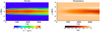 |
Fig. 2. Time-distance plot of the density (left) and temperature (right) at the apex of the loop (z = 100 Mm and x = 0 Mm). |
2.3. MUSE synthetic emission
The Multi-Slit Solar Explorer (MUSE) mission, due to launch in 2027, aims to deliver the high spatial resolution and temporal cadence necessary to understand the physical mechanisms of coronal heating (De Pontieu et al. 2020, 2022; Cheung et al. 2022). MUSE will consist of a multi-slit extreme-ultraviolet (EUV) spectrograph and context imager. By obtaining spectra from four EUV lines (Fe IX 171 Å, Fe XV 284 Å, Fe XIX 108 Å, and Fe XXI 108 Å) along 37 slits, MUSE will simultaneously capture spectroscopic snapshots of coronal and transition region plasma.
To investigate the accuracy and robustness of the wave identifiers when applied to observational data, we generated MUSE Fe IX synthetic spectra from the numerical data. The Fe IX passband captures temperatures of about 0.6 to 1.5 MK (e.g. Krucker et al. 2011). In the numerical simulation, the temperature was initially 1 MK, and the plasma was heated to a mean of 1.1 MK with a maximum temperature of just below 1.8 MK in the loop boundary. Therefore, most of the simulation is captured by this passband. As illustrated in Fig. 3, we generated synthetic emission data for three different lines of sight (LOS) integrated along the x-, y-, and z-axis of the numerical simulation and corresponding to the direction perpendicular to the oscillation, parallel with the oscillation and along the loop, respectively.
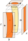 |
Fig. 3. Illustration of the three LOS considered in this paper. The transverse oscillations will be visible as actual loop displacements in the x- and z-LOS. |
2.4. Observational data
In the optically thin corona, spectroscopic data provide LOS-integrated intensities, Doppler velocities, and line widths. This presents a challenge because the wave identifiers νA, ν∥ and ν⊥ require the curl and divergence of the velocity and the direction of the magnetic field (about which we have limited information).
In our setup, the transverse wave in the y-direction will be apparent as a displacement of the loop in the plane-of-the-sky intensity in the x- and z-LOS, but not in the y-LOS. In the x- and z-LOS, for any displacement Δy observed over a time step Δt, we can estimate vy = Δy/Δt. Assuming the magnetic field is frozen-in to the plasma and is tangential to the loop, we can deduce By in a similar way. In Table 1 we list the velocity components that we either observed directly or can estimate from each LOS. For each LOS, we always have the Doppler velocity as a function of the perpendicular plane coordinate system.
Derivatives that can be obtained from each LOS.
Even if all three LOS were available, it would not be possible to calculate all nine velocity derivatives needed to estimate the fast and slow identifiers (ν⊥ and ν∥). However, the Alfvén identifier (νA) only requires the components off the main diagonal in Table 1. In this study, we present two ways to estimate νA. Firstly, in Sect. 3.2, we assume that the observational data are along the LOS parallel to the oscillation (the y-LOS). Here, we can deduce νA accurately from this single LOS. Secondly, in Sect. 3.3, we assume that we have the two LOS that are not parallel to the oscillation, and we demonstrate how νA can be estimated using loop tracking.
3. Results
3.1. Wave identifiers in numerical data
Before we applied the wave identifiers to the synthetic emission, we applied them directly to the original numerical simulation data. Figures 4 and 5 show time-distance plots of the Alfvén, νA, and fast, ν⊥, identifier at the loop apex (y = 0 Mm and z = 100 Mm) in the range x ∈ [ − 2, 2] Mm. For the fast identifier (Fig. 4), the magnitude is greatest at the centre of the loop, but it decreases with time. The reason is that the global kink mode decays as a result of the energy transfer to azimuthal Alfvén waves in the loop boundary (Ionson 1978). This is reflected in the time-distance plot of the Alfvén identifier in Fig. 5, where the magnitude of the Alfvén identifier gradually increases with time in the loop boundary (x ≈ ±1 Mm). The non-zero regions of the Alfvén identifier also broaden into the interior of the loop as a result of the disruption of the loop cross section at later times (e.g. middle row of Fig. 7 in De Moortel & Howson 2022). The signatures of the Alfvén waves are clearly visible in vertical and horizontal cross sections of νA (left panels of Figs. 6 and 8, respectively) as distinct positive or negative bands at x = ±1 Mm.
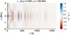 |
Fig. 4. Time-distance plot of the numerical simulation ν⊥ along y = 0 Mm, z = 100 Mm for x ∈ [ − 2, 2] Mm. |
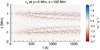 |
Fig. 5. Time-distance plot of the numerical simulation νA along y = 0 Mm, z = 100 Mm for x ∈ [ − 2, 2] Mm. |
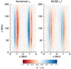 |
Fig. 6. Alfvén identifier νA for numerical data (left) and the MUSE synthetic emission (right) at t = 193 s. For the synthetic emission, |

3.2. Synthetic emission data. Single line of sight
When we assume that one can observe the loop from the direction parallel to the oscillation (y-LOS), the observed Doppler velocity, vy(x, z), coincides with the oscillation. Along this LOS, we do not observe any oscillation in the intensity, and because the field is approximately frozen into the plasma, we assumed Bx = 0 G. Because the wave amplitude is relatively small, the component of the field induced by the oscillation will be small in comparison to the background field. Thus, we assumed that the field is parallel to the initial loop axis (z-direction) throughout the simulation. Lastly, we assumed vx = 0 and ∂vx/∂y = 0 because we do not observe any velocity perturbation in the x-direction. Hence, the synthetic emission Alfvén identifier reduces to νA = ∂vy/∂x.
In Fig. 6, we compare the Alfvén identifier for the numerical simulation (left panel) and the synthetic emission (right panel). For the numerical simulation, we show the y = 0 Mm plane, while the synthetic emission is integrated over the y-LOS. It is clear that νA calculated from the synthetic emission captures the nature of the numerical data well. In both panels, we see vertical bands with the same signs and roughly the same magnitude in the loop boundaries (around x = ±1 Mm), where the azimuthal Alfvén waves develop due to resonant absorption.
Moreover, the synthetic emission captures the numerical behaviour in the time-distance plot in Fig. 7, which shows the cross section at z = 100 Mm over time. There are clear oscillations in the boundary that expand into the loop interior, matching the corresponding numerical simulation νA plot in Fig. 5.
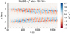 |
Fig. 7. Time-distance plot of the synthetic emission |

So far, we considered the particular case in which the LOS coincides with the dominant direction of the oscillation. Along the x-LOS, the oscillation would be visible as a periodic loop displacement. However, for the x-LOS, we do not have vy(x), which provides the dominant derivative in νA. If, as we did above, we assume that the velocity derivative we do not observe is zero, that is, ∂vy/∂x = 0, then we obtain a synthetic emission νA with little correspondence to the numerical simulation νA.
3.3. Synthetic emission data. Multiple lines of sight
As stated above, we can estimate νA from the y-LOS emission (i.e. the LOS parallel to the oscillation), but not from any other single LOS. However, when we have both the x- and z-LOS, we can use loop tracking (see Appendix B) to deduce vy(y, z) vy(x, y) and By = BzΔy/Δz. Our expression for the Alfvén identifier now becomes νA = (∂vx/∂z − ∂vz/∂x)By + (∂vy/∂x − ∂vx/∂y)Bz. The loop-tracking algorithm works best before the loop becomes significantly deformed by the KHI, that is, the first 400 seconds. In Fig. 8 we show the Alfvén identifier in the xy-plane for the numerical simulation (left) and synthetic emission (right) at t = 203 s. The numerical data νA are taken at a horizontal cut at z = 100 Mm (loop apex). The synthetic emission νA is derived using the x- and z-LOS simultaneously.
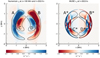 |
Fig. 8. Horizontal cut of νA at z = 100 Mm for the numerical simulation (left) and synthetic emission (right). The labelled contours highlight areas of predominantly negative or positive νA values. |
Although it is more complex, the synthetic emission νA displays the same large-scale features (outlined by the black contours) as the numerical simulation. For example, regions A and B are predominantly positive and negative, as are the corresponding regions A* and B* in the synthetic emission results (right panel). Although they are approximately cospatial, we note that the areas are not identical between the two panels. This is due to the compression of the loop and associated errors from the loop-tracking algorithm (see the discussion below). The A (A*) and B (B*) regions correspond to the azimuthal Alfvén waves in the boundary of the loop, which are clearly visible in the vertical cuts discussed earlier (Fig. 5 and left panel of Fig. 6).
Clearly, the agreement between the numerical measurements and the synthetic estimates of νA is not perfect. There are several reasons for this, including integration over the entire loop length (due to the optically thin plasma) for the synthetic emission case. Further, inherent to the loop-tracking method (see Appendix B) is the assumption that the displacement evolves linearly between the two time steps (i.e. the velocity is constant). However, as the cadence (∼19 s) is relatively long (but comparable to existing instruments), the velocity is not constant over the interval, and this can lead to differences in the estimated velocities compared to the numerical values.
Figure 9 shows a time-distance plot of the synthetic emission νA at y = 0 Mm. We overplot the outlines of the simulation νA (at y = 0 Mm and z = 100 Mm), where the solid and dotted lines enclose negative and positive values, respectively. Although there is some additional fine-scale structuring, clear oscillations between positive and negative values are visible in the loop boundary for the synthetic emission νA. These oscillations, including the broadening into the loop, correspond to the location of the same oscillations as in the numerical simulation νA.
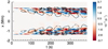 |
Fig. 9. Time-distance plot of the synthetic emission νA based on two LOS at y = 0 Mm. The numerical simulation νA at y = 0 Mm and z = 100 Mm is overplotted (black contours), where the solid lines enclose negative values and the dotted lines enclose positive values of νA. |
4. Discussion and conclusion
We have focused on the wave identifiers νA and ν⊥ from Eqs. (1) and (3) in a numerical simulation of a transversely oscillating coronal loop. We have shown that in a numerical simulation, the fast identifier, ν⊥, isolates the global transverse oscillation of the loop and the decay of the kink-mode due to resonant absorption. We also showed that the Alfvén identifier, νA, picks up the simultaneous excitation of azimuthal Alfvén waves in the loop boundary.
The synthetic emission data allowed us to provide a proof of concept of the applicability of the Alfvén identifier for observational data. In the particular case when the LOS is parallel to the direction of oscillation, the oscillation would not be observed as a physical displacement of the loop axis, but only as a periodic variation in the Doppler shift. However, because ∂vy/∂x is the dominant term in νA (for this model), the agreement between the Alfvén identifier calculated from the simulation and that estimated from the synthetic emission is good.
In the more general case when the LOS does not align with the direction of the oscillation, a single LOS is not sufficient to calculate any of the wave identifiers. However, as we have demonstrated, the Alfvén identifier could still be estimated if a second LOS were available to observe the loop at a different angle. We considered the case of two LOS, one perpendicular to both the loop axis and the polarisation of the kink wave, and the other along the loop. This allowed us to estimate νA by tracking the loop displacement from intensity data alone (no spectroscopic requirement). Observations like this would require coordination between different telescopes, for example, a combination of an Earth-orbiting telescope, such as MUSE, Hinode, or Interface Region Imaging Spectrograph (IRIS), and a second spacecraft orbiting the Sun, such as Solar Orbiter. In reality, simultaneous imaging is unlikely to be available from two perpendicular LOS, and a combination of spectroscopic data and imaging may be required. We will investigate the feasibility of this approach in future studies.
The loop-tracking algorithm we used requires the loop profile to remain coherent, which for this specific simulation worked well for the first 400 seconds, when the loop profile was substantially disrupted by the KHI. However, even at early times, we find some inaccuracies in the velocity estimates. These are due to compression and rarefaction at the leading and trailing edges of the loop and (as discussed in Appendix B) because of the relatively poor cadence in comparison to the oscillation period (chosen to be comparable to the cadence of modern telescopes).
As this current study is intended as a proof of concept, we only considered one set of model parameters. Hence, further investigation into the performance of the wave identifiers with different values for, for instance, the wave driver amplitude, the magnetic field, and the density profile is required to understand their robustness. Lastly, the synthesised emission contained only a single structure along any LOS, and no noise was added to the data. Real observations will inevitably contain multiple (other) structures along the LOS and noise from instrumental effects, for example, which will likely impact the estimates of the derivatives. Therefore, it would be useful in a future study to quantify how much useful information can be extracted for different signal-to-noise ratios. However, in our relatively simplistic setup, we showed two instances for which it would be possible to ascertain the Alfvén identifier. Therefore, we conclude that under suitable conditions, it may be possible to use this method to classify different wave modes in observations of the solar corona.
Acknowledgments
E.E. received funding from the University of St Andrews Global Fellowship Scheme. I.D.M. received funding from the Research Council of Norway through its Centres of Excellence scheme, project number 262622.
References
- Arber, T. 2021, https://github.com/Warwick-Plasma/Lare3d [Google Scholar]
- Arregui, I. 2015, Philos. Trans. R. Soc. London Ser. A, 373, 20140261 [Google Scholar]
- Banerjee, D., Krishna Prasad, S., Pant, V., et al. 2021, Space Sci. Rev., 217, 76 [NASA ADS] [CrossRef] [Google Scholar]
- Cheung, M. C. M., Martínez-Sykora, J., Testa, P., et al. 2022, ApJ, 926, 53 [NASA ADS] [CrossRef] [Google Scholar]
- De Moortel, I., & Howson, T. A. 2022, ApJ, 941, 85 [NASA ADS] [CrossRef] [Google Scholar]
- De Pontieu, B., Martínez-Sykora, J., Testa, P., et al. 2020, ApJ, 888, 3 [NASA ADS] [CrossRef] [Google Scholar]
- De Pontieu, B., Testa, P., Martínez-Sykora, J., et al. 2022, ApJ, 926, 52 [NASA ADS] [CrossRef] [Google Scholar]
- Edwin, P. M., & Roberts, B. 1983, Sol. Phys., 88, 179 [Google Scholar]
- Goossens, M., Doorsselaere, T. V., Soler, R., & Verth, G. 2013, ApJ, 768, 191 [NASA ADS] [CrossRef] [Google Scholar]
- Howson, T. 2022, Symmetry, 14, 384 [NASA ADS] [CrossRef] [Google Scholar]
- Ionson, J. A. 1978, ApJ, 226, 650 [NASA ADS] [CrossRef] [Google Scholar]
- Khomenko, E., & Cally, P. S. 2011, J. Phys. Conf. Ser., 271, 012042 [NASA ADS] [CrossRef] [Google Scholar]
- Khomenko, E., & Cally, P. S. 2012, ApJ, 746, 68 [Google Scholar]
- Krucker, S., Raftery, C. L., & Hudson, H. S. 2011, ApJ, 734, 34 [NASA ADS] [CrossRef] [Google Scholar]
- Leenaarts, J., Carlsson, M., & van der Voort, L. R. 2015, ApJ, 802, 136 [NASA ADS] [CrossRef] [Google Scholar]
- McIntosh, S. W., de Pontieu, B., Carlsson, M., et al. 2011, Nature, 475, 477 [Google Scholar]
- Nakariakov, V. M., & Kolotkov, D. Y. 2020, ARA&A, 58, 441 [Google Scholar]
- Nakariakov, V. M., & Verwichte, E. 2005, Liv. Rev. Sol. Phys., 2, 3 [Google Scholar]
- Parnell, C. E., & De Moortel, I. 2012, Philos. Trans. R. Soc. London Ser. A, 370, 3217 [Google Scholar]
- Raboonik, A. 2022, Ph.D. Thesis, Monash University, Australia [Google Scholar]
- Shelyag, S., Khomenko, E., de Vicente, A., & Przybylski, D. 2016, ApJ, 819, L11 [Google Scholar]
- Srivastava, A. K., Ballester, J. L., Cally, P. S., et al. 2021, J. Geophys. Res. (Space Phys.), 126, e029097 [NASA ADS] [Google Scholar]
- Tomczyk, S., McIntosh, S. W., Keil, S. L., et al. 2007, Science, 317, 1192 [Google Scholar]
- Van Doorsselaere, T., Srivastava, A. K., Antolin, P., et al. 2020, Space Sci. Rev., 216, 140 [Google Scholar]
- Wilmot-Smith, A. L. 2015, Philos. Trans. R. Soc. London Ser. A, 373, 20140265 [Google Scholar]
- Yadav, N., Keppens, R., & Braileanu, B. P. 2022, A&A, 660, A21 [NASA ADS] [CrossRef] [EDP Sciences] [Google Scholar]
Appendix A: Setup of the numerical model
The numerical simulation discussed in this Letter was first presented by De Moortel & Howson (2022). The authors modelled a coronal loop as a 3D flux tube with parameters representative of the quiet-Sun corona. For simplicity, the flux tube was straightened, where the z-axis in the simulation is aligned with the loop axis (see Fig. 1). The numerical grid consisted of 512 × 512 × 100 grid points, where −4 ≤ x, y ≤ 4 Mm and 0 ≤ z ≤ 200 Mm. The initial density profile was given by
where  . The values ρe and ρi are the exterior and interior densities of the loop, respectively. The constants a and b define the radius of the flux tube and the width of the boundary layer, respectively, and were selected such that the loop had a radius of 1 Mm and the boundary layer was approximately 0.4 Mm thick. Initially, the exterior density was ρe = 1.67×10⁻¹³ kg/m3 and ρi = 3ρe (see Fig. 1), and the temperature was initially 1 MK everywhere. The background magnetic field was aligned with the z-axis and had a field strength of 30 G, with a small reduction ( 0.7%) in the loop interior to maintain total pressure balance.
The simulation was performed using Lare3D (Arber 2021), which advances the fully 3D resistive MHD equations in normalised form. The equations are given by


where ρ is the plasma pressure, v is the velocity, j is the normalised current density, B is the magnetic field, P is the gas pressure, and ϵ is the specific internal energy. The viscosity was included in the momentum equation in the form of a viscous force, Fvisc. The energy equation contains terms for the optically thin radiation (Λ(T)), uniform background heating (Qbg), and viscous heating (Qvisc). The background heating term was chosen to balance the radiative losses in the exterior environment, that is, to maintain the temperature of 1 MK in the low-density part of the loop. Radiative losses will be stronger in the higher-density interior of the loop, and hence, the background heating is not enough to balance the radiative losses inside the flux tube. Therefore, without any additional heating (e.g. from the dissipation of wave energy), the loop is expected to cool.
The x and y boundaries were set to be periodic. At the lower-z boundary, a transverse wave driver of the form vy = v0sin(ωt) was imposed. Here, v0 is the amplitude, and it was set to approximately 8 km/s, and ω is the wave frequency, set to the natural kink frequency (see e.g. Edwin & Roberts 1983; Nakariakov & Verwichte 2005), with the resonant period being 86.3 s. A reflecting upper boundary ensured that the fixed-frequency wave driver excited the fundamental kink mode in the system.
Appendix B: Loop tracking and magnetic field approximation
In this appendix, we outline the process we used to estimate the velocity vy and the magnetic field By based on tracking the displacement (Δy) of the loop in the y direction. For the velocity, we used the displacement in time, while the magnetic field estimate was based on the displacement in space (i.e. how the loop changes with z). We describe the algorithm for deducing vy from the x-LOS, but the same method was used to calculate vy from the z-LOS and By from the x-LOS.
From the x-LOS, everything is projected onto the yz-plane, and through this, the intensity Ix(t, y, z) is known. For this initial study, we assumed that the intensity is a smooth function with only one clear maximum (i.e. Gaussian-like). For our simulation, this assumption holds for relatively early times (t < 400 s) before the loop cross section is substantially deformed by the KHI. To track the loop displacement at each height z, we used the relative values of the intensity at this height at different time steps. For example, we matched 10% of the maximum intensity at time step t1 to 10% of the maximum intensity at time step t2, and so on. We repeated this on either side of the loop to ensure that we tracked the full loop profile. This process gives the Δyi as illustrated in Figure B.1. The loop tracking in this study was based on n = 100 intensity intervals and was repeated for each value of z. The estimate of the velocity vy(y, z) at time t = (t1 + t2)/2 was based on these displacements Δyi.
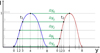 |
Fig. B.1. Loop tracking to derive the displacements. For clarity, we only show a selection of the Δy’s. |
An artefact of this loop-tracking algorithm are the distinct outer edges that are evident in Fig 8 (right panel). They can be ignored when the synthetic νA is compared with the numerical data. This artefact arises when the velocity is estimated only for the loop (where the displacement is evident) and not for the rest of the domain, where we set vy = 0 m/s. This causes an abrupt change in the loop boundary between vy = 0 and vy ≠ 0, which in turn means that the derivatives of vy will be artificially large at this location.
To estimate the magnetic field, we assumed that it was frozen-in to the oscillating loop and that the background field was uniform and aligned with the z direction. Because there is no visible motion in the x direction, we assumed Bx = 0. To estimate By, we employed a method similar to what we used to find vy, but instead of calculating the displacement in time, we tracked the position of the loop as a function of z. Because we assumed that the field is tangential to the loop, we obtained By = BzΔy/Δz.
All Tables
All Figures
|
Fig. 1. Vertical cut (top) and horizontal cross section (bottom) of the initial density (i.e. at t = 0 s) both at y = 0 Mm. |
| In the text | |
|
Fig. 2. Time-distance plot of the density (left) and temperature (right) at the apex of the loop (z = 100 Mm and x = 0 Mm). |
| In the text | |
|
Fig. 3. Illustration of the three LOS considered in this paper. The transverse oscillations will be visible as actual loop displacements in the x- and z-LOS. |
| In the text | |
|
Fig. 4. Time-distance plot of the numerical simulation ν⊥ along y = 0 Mm, z = 100 Mm for x ∈ [ − 2, 2] Mm. |
| In the text | |
|
Fig. 5. Time-distance plot of the numerical simulation νA along y = 0 Mm, z = 100 Mm for x ∈ [ − 2, 2] Mm. |
| In the text | |
|
Fig. 6. Alfvén identifier νA for numerical data (left) and the MUSE synthetic emission (right) at t = 193 s. For the synthetic emission, |
| In the text | |
|
Fig. 7. Time-distance plot of the synthetic emission |
| In the text | |
|
Fig. 8. Horizontal cut of νA at z = 100 Mm for the numerical simulation (left) and synthetic emission (right). The labelled contours highlight areas of predominantly negative or positive νA values. |
| In the text | |
|
Fig. 9. Time-distance plot of the synthetic emission νA based on two LOS at y = 0 Mm. The numerical simulation νA at y = 0 Mm and z = 100 Mm is overplotted (black contours), where the solid lines enclose negative values and the dotted lines enclose positive values of νA. |
| In the text | |
|
Fig. B.1. Loop tracking to derive the displacements. For clarity, we only show a selection of the Δy’s. |
| In the text | |
Current usage metrics show cumulative count of Article Views (full-text article views including HTML views, PDF and ePub downloads, according to the available data) and Abstracts Views on Vision4Press platform.
Data correspond to usage on the plateform after 2015. The current usage metrics is available 48-96 hours after online publication and is updated daily on week days.
Initial download of the metrics may take a while.