| Issue |
A&A
Volume 690, October 2024
|
|
|---|---|---|
| Article Number | A202 | |
| Number of page(s) | 8 | |
| Section | The Sun and the Heliosphere | |
| DOI | https://doi.org/10.1051/0004-6361/202451196 | |
| Published online | 10 October 2024 | |
Can we rely on EUV emission to identify coronal waveguides?
1
Rosseland Centre for Solar Physics, University of Oslo, P.O. Box 1029 Blindern, NO-0315 Oslo, Norway
2
Institute of Theoretical Astrophysics, University of Oslo, P.O. Box 1029 Blindern, NO-0315 Oslo, Norway
3
Department of Mathematics, Physics and Electrical Engineering, Northumbria University, Newcastle Upon Tyne NE1 8ST, UK
Received:
20
June
2024
Accepted:
13
August
2024
Abstract
Context. Traditional models of coronal oscillations rely on a modelling of the coronal structures that support them as compact cylindrical waveguides. An alternative model of the structure of the corona has recently been proposed, in which the thin strand-like coronal loops, that are observed in the extreme-UV (EUV) emission are the result of the line-of-sight integration of warps in more complex coronal structures. This is referred to as the coronal veil model.
Aims. We extend the implications of the coronal veil model of the solar corona to models of coronal oscillations.
Methods. Using convection-zone-to-corona simulations with the radiation-magnetohydrodynamics (rMHD) code Bifrost, we analysed the structure of the self-consistently formed simulated corona. We focused on the spatial variability of the volumetric emissivity of the Fe IX 171.073 Å EUV line and on the variability of the Alfvén speed, which captures the density and magnetic structuring of the simulated corona. We traced features associated with large magnitudes of the Alfvén speed gradient, which trap MHD waves and act as coronal waveguides. We searched for the correspondence with emitting regions, which appear as strand-like loops in the line-of-sight-integrated EUV emission.
Results. We find that the cross sections of the waveguides bounded by large Alfvén speed gradients become less circular and more distorted with increasing height in the solar atmosphere. The waveguide filling factors corresponding to the fraction of the waveguides filled with plasma that emits in the given EUV wavelength range from 0.09–0.44. This suggests that we can only observe a small fraction of the waveguide. Similarly, the projected waveguide widths in the plane of the sky are several times larger than the widths of the apparent loops that are observed in the EUV.
Conclusions. We conclude that the coronal veil structure is independent of the model. As a result, we find a lack of straightforward correspondence between peaks in the integrated emission profile that constitute apparent coronal loops and regions of plasma bound by a large Alfvén speed gradient that act as waveguides. Coronal waveguides cannot be reliably identified based on emission in a single EUV wavelength is not reliable in the simulated corona formed in convection-zone-to-corona models.
Key words: magnetohydrodynamics (MHD) / Sun: corona / Sun: magnetic fields / Sun: oscillations
Corresponding author; This email address is being protected from spambots. You need JavaScript enabled to view it.
© The Authors 2024
 Open Access article, published by EDP Sciences, under the terms of the Creative Commons Attribution License (https://creativecommons.org/licenses/by/4.0), which permits unrestricted use, distribution, and reproduction in any medium, provided the original work is properly cited.
This article is published in open access under the Subscribe to Open model. This email address is being protected from spambots. You need JavaScript enabled to view it. to support open access publication.
1. Introduction
Coronal loops are the basic building blocks of the solar corona. They are the thin strand-like structures that are most commonly observed in extreme-ultraviolet (EUV) and soft X-ray (SXR) emission. They correspond to the coronal plasma that is confined inside magnetic structures and therefore traces the topology of the coronal magnetic field. This gives coronal loops an arch-like appearance, with typical lengths from tens to some hundred megameters (Reale 2014). They are typically few hundred kilometers in the diameter, but higher-resolution observations with instruments such as Hi-C and the High-Resolution Imager (HRI) of the Extreme Ultraviolet Imager (EUI) of Solar Orbiter have revealed fine-scale coronal loop structure that was previously unresolved by comparably lower-resolution imagers such as the Atmospheric Imaging Assembly on board the Solar Dynamics Observatory (SDO/AIA) (Peter et al. 2013; Williams et al. 2020; Antolin et al. 2023). Cool tracers of the coronal magnetic field such as coronal rain (Antolin & Rouppe van der Voort 2014; Kohutova & Verwichte 2016) observable by high-resolution ground-based instruments provide further insight into the fine scale structure of the corona (Scullion et al. 2014).
The solar corona is a dynamic environment, and the coronal magnetic field continuously changes and evolves. Recent observational evidence suggests complex density structuring (Berghmans et al. 2023). Simplified models of static coronal loops neglect this spatial and temporal variability of the solar atmosphere. In order to account for realistic magnetic field configurations and density structuring in the solar corona, a more self-consistent approach to modelling the evolution of coronal structures is necessary. One such approach involves using self-consistent convection-zone-to-corona simulations, in which the structuring and the evolution of the corona is driven entirely by the dynamics of the lower solar atmosphere. It can be therefore argued that the simulated corona that forms in these models is more realistic.
The structure of the corona in these models has been analysed by Malanushenko et al. (2022), who investigated the relation between integrated synthetic EUV emission and the three-dimensional structure of the volumetric emissivity using a self-consistent MURaM simulation. In contrast to the popular image of coronal loops as well-defined plasma cylinders that are clearly distinct from the surroundings, the emitting structures seen in this type of models are much more complex, and the strand-like appearance of coronal loops visible in the synthetic EUV emission comes from wrinkles in these shapes that are integrated along the line of sight, similar to folds in a veil. This coronal veil structure is present in other convection-zone-to-corona models, including Bifrost models (Gudiksen et al. 2011), and it therefore appears to be independent of the model. It is worth noting that even simple three-dimensional MHD coronal models of transverse wave propagation along flux tubes that generate shear-flow instabilities (e.g. Kelvin-Helmholtz; KH) can produce strand-like structures through the compressive physical processes of the KH roll-ups (Antolin et al. 2014). Hence, the fine-scale structure of the corona can be independent of the motions of the footpoints of flux tubes at photospheric or chromospheric heights.
In the case of oscillations in coronal structures, the coronal loops act as waveguides, in which the inhomogeneity of physical properties provides a boundary that often leads to an onset of standing modes in the structures. The waveguide boundaries are determined by the transverse variation in the density at the loop edges, or more generally, by the variation in the Alfvén speed (Nakariakov et al. 1996).
The classical model for coronal oscillations relies on the magnetised cylinder model (Edwin & Roberts 1983) and assumes that the individual coronal loops have approximately circular cross sections and are to a large degree decoupled from the surrounding background plasma. This model forms the basis for coronal seismology, which is a widely used method that employs coronal oscillation parameters for diagnostics of physical properties of the coronal plasma that are otherwise difficult to measure directly, such as coronal densities and magnetic fields (Nakariakov & Kolotkov 2020). The complexity of the coronal structure seen in self-consistent models of the solar atmosphere, however, clearly contradicts this simplified picture. The impact of the coronal veil structure on the accuracy of coronal seismological methods that are largely based on the magnetic cylinder approximation for coronal loops is still not clear.
In this paper, we analyse the structure of the corona in a three-dimensional convection-zone-to-corona simulation using the radiation-MHD code Bifrost. We aim to identify the waveguides in the coronal veil based on the variation in the Alfvén speed in three dimensions, and match them to the strand-like features that appear in the forward-modelled EUV emisssion. This tells us how valid our approximations about the 3-dimensional structure of oscillating coronal loops are.
2. Numerical model
We analysed the structure of the corona that formed in the numerical simulation of a magnetically enhanced network spanning from the upper convection zone to the coronal heights using the radiation-MHD code Bifrost (Gudiksen et al. 2011). Bifrost is a radiation-MHD code that solves resistive MHD equations on a staggered Cartesian grid. Built on top of the Stagger code (Stein et al. 2024), it includes radiative transfer with scattering in the photosphere and lower chromosphere and parameterised radiative losses and heating in the upper chromosphere, transition region, and corona. The simulation used in this work also accounts for field-aligned thermal conduction and non-equilibrium ionisation of hydrogen in the equation of state. The size of the numerical box was 24 × 24 × 16.8 Mm spanning from 2.4 Mm below the photosphere to 14.4 Mm in the corona, and the grid resolution was 504 × 504 × 496. The simulation boundary conditions were periodic in the x and y directions and open in the z direction. The top boundary used characteristic boundary conditions, designed to transmit disturbances with minimum reflection (Gudiksen et al. 2011). The flows were allowed to pass through the bottom boundary, and the magnetic field wass passively advected – no additional magnetic field was introduced into the domain. The numerical setup is described in more detail in Kohutova et al. (2023). The analysed snapshot corresponds to the t = 980 s time step of the extended simulation run described therein. In this model, the coronal evolution and heating is driven by the dynamics of the lower solar atmosphere and the associated convective motions. The high coronal temperatures are maintained primarily through Joule and viscous heating associated with magnetic braiding. The heating in the vast majority of the domain is hence self-consistent. The temporal variability of the simulated corona is significantly more complex than in more idealised models, as the footpoints of the magnetic structures are dragged around by the convective motions. Similarly, the coronal structure is driven by the dynamics of the lower solar atmosphere; the magnetic configuration is initialised from two opposite-polarity patches that are quickly swept into the intergranular lanes by the convective downflows. The structure of the corona is therefore free from a priori assumptions about the shape of the coronal loops. There are several coronal structures with densities higher than the surrounding plasma. These are filled by the chromospheric evaporation in response to heating events (e.g. Kohutova et al. 2020).
To analyse the appearance of the coronal loops in the model in EUV, we calculated the synthetic emission in the Fe IX 171.073 Å coronal line. The emission intensity Iλ for the optically thin coronal EUV lines corresponds to the integral of the volumetric emissivity at the specific wavelength along the line of sight:
 (1)
(1)
where ϕλ is the Gaussian line profile accounting for the Doppler shift due to the velocity along the line-of-sight (LOS) and for the thermal line broadening, and ϵλ0 is the volumetric emissivity of the given spectral line at the rest wavelength,
 (2)
(2)
Here, ne is the electron density, T is the plasma temperature, and Gλ0 is the contribution function of the specific spectral line calculated using the CHIANTI atomic database v.10 (Del Zanna et al. 2021). We calculated Gλ0 values of the Fe IX 171.073 Å coronal line on a 200 × 3000 grid of temperatures and densities to create a look-up table for speeding up the calculation. We do this for the temperature range from log T = 4.0 to log T = 7.0 and for the density range log ne = 8 to log ne = 11 (in cgs units). We then used cubic spline interpolation in T and zero-order interpolation in ne to determine the value of GFeIX and subsequently ϵλ0 at each simulation grid point. As we are interested in the three-dimensional structure of the coronal EUV emission, ϵFeIX is the main quantity on which we focus in the analysis below.
3. Coronal waveguides
We used the 3-dimensional volumetric Fe IX emissivity to examine the coronal structures in the simulation. Vertical slices across the simulation domain at x = 13 Mm showing the structure of the plasma density, temperature, and the corresponding volumetric emissivity, along with the line-of-sight (LOS) integrated Fe IX emission in the x–z plane are shown in Fig. 1. The synthetic LOS-integrated emission contains several coronal loops, which are aligned with the magnetic field connecting the two magnetic polarity patches at z = 0 Mm. We partially marked the axis outline of five distinct loops and label them A–E. The width of the coronal loops varies from ∼1 Mm for the more diffuse loops (e.g. loop E) to 200 km for the most fine-scale strands (loop B). The coronal structure visible in the x = 13 Mm slice across the coronal loops shows complex wrinkled surfaces and does not contain clearly defined loop cross sections. The transverse structuring of the coronal loops is consistent with the coronal veil interpretation discussed by Malanushenko et al. (2022). The temperature and density structure in the identical slices follows the complex shapes seen in the emissivity slice.
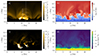 |
Fig. 1. Coronal structure in the simulation. We show the LOS-integrated Fe IX emission intensity in the x–z plane (a). The dashed line at x = 13 Mm marks the y–z plane along which the subsequent slices are taken. The dotted lines mark a portion of the loop axis for loops A–E. Vertical slices taken across the coronal loops at x = 13 Mm show the plasma temperature (b), volumetric emissivity (c), and the plasma density (d). |
To cross-correlate the loops visible in the LOS-integrated emission with the emitting features in the volumetric emissivity, we examined the emission profile along the dashed line intersecting the loops that are visible in the synthetic EUV emission at the apex (Fig. 2). The local peaks in the emission profile were matched to the loops marked in Fig. 1. The z-coordinates of the loop boundaries were then plotted over the x = 13 Mm emissivity slice to highlight the emitting features that contribute to peaks A–E when integrated along the y-axis. We find that multiple coronal structures with varying y-coordinates contribute to a single peak in the emission profile, which we identify as a single loop, due to the LOS superposition. We note that the features located at lower coronal heights have a very high degree of LOS superposition, which subsequently decreases at greater coronal heights. We highlight the dominant contributing emission regions corresponding to each loop. The dominant features in the EUV emissivity have irregular shapes, and the cross-sections of the corresponding coronal structures therefore cannot be approximated as circular.
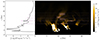 |
Fig. 2. Vertical slice across the volumetric emissivity at x = 13 Mm (right), and the corresponding x = 13 Mm LOS-integrated emission profile (left). The local emission peaks corresponding to the loops A–E are marked by dashed purple lines. These also mark the z-coordinates of the contributing regions in the emissivity slice. The dominant emitting regions corresponding to each loop are marked by purple rectangles. |
We show the full three-dimensional rendering of the volumetric emissivity in Fig. 3 together with the associated animation, which demonstrates the line-of-sight effects when viewing the entire simulation domain from different directions. Several features with enhanced emissivity aligned with the coronal magnetic fields are clearly visible in the simulation domain, with a varying thickness and complex cross-sections. In particular, we find that the primary contributing sources to features with strand-like appearance in the LOS-integrated EUV emission in the x–z plane are thin sheet-like structures with elongated spatial extent in the y-direction (this is most prominent for loops A, B and C).
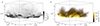 |
Fig. 3. Three-dimensional rendering of |∇vA| (a) and the volumetric emissivity ϵFe IX (b). An animation is available online. |
We further determined the variation in the Alfvén speed  in the simulated corona by calculating the Alfvén speed gradient ∇vA, which highlights the regions with inhomogeneities in the physical properties of the coronal plasma acting as waveguide boundaries (Fig. 3). The spatial distribution of |∇vA| in the simulation domain has a similar veil-like structure as the EUV emissivity, and the regions with the strongest |∇vA| form coherent surfaces extending across several megameters, suggesting that the regions in the corona acting as individual waveguides have a large spatial extent and complex shapes. Fig. 4 shows the variation in the structures corresponding to enhanced |∇vA| with height. In the figure, we show the horizontal slices of |∇vA| at three different heights at z = 2 Mm corresponding to the loop footpoints close to the transition region, at z = 5 Mm corresponding to the loop legs in the lower corona, and at z = 10 Mm at coronal heights corresponding to the location of the loop apex (this is only approximate, as the loop tops are extensive, see Fig. 3). The associated animation shows the transition through the entire solar atmosphere starting from the photosphere at z = 0 Mm to the upper boundary of the simulation domain. This highlights how the footpoints of the structures defined by enhanced |∇vA| transition from well-defined, albeit irregular closed cross-sections at z = 2 Mm in the transition region into the veil-like structure at coronal heights at z = 10 Mm.
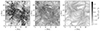 |
Fig. 4. Horizontal slices across |∇vA| at z = 2 Mm (a) z = 5 Mm (b) and z = 10 Mm (c). An animation is available online. |
In order to determine the characteristics of the individual waveguides that are associated with coronal loops A–E, or rather, with the source regions responsible for the appearance of the loops, we plot the x = 13 Mm slice through |∇vA| (Fig. 5). We trace the edges visible in the |∇vA| plot while identifying enclosed shapes that form the waveguide cross-section in the x = 13 slice overlapping the loop emission source regions marked in Fig. 2 (also shown by emissivity contours in Fig. 5). We then trace the magnetic connectivity of the waveguide boundaries to obtain the full three-dimensional structure of each waveguide. We terminate the integration of B at z = 1.5 Mm, as below this height there is no emission in the coronal lines. We note that the |∇vA| varies along the waveguide boundaries (although not as strongly as across the waveguide boundaries), which complicates a separation in places with weaker gradients.
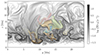 |
Fig. 5. x = 13 Mm slice across |∇vA|. The cross sections of waveguides encompassing dominant emitting regions for each loop are shown in blue (waveguide 1), green (waveguide 2), orange (waveguide 3), and red (waveguide 4). The emissivity contours are overplotted. |
Fig. 6 shows cuts across the volumetric emissivity and the corresponding waveguide cross-sections along different planes corresponding to the loop footpoints close to the transition region, loop legs in the lower corona, and the coronal loop apex. The full three-dimensional structure of the waveguides is shown in Fig. 7. Even though some of the boundaries of the strong emissivity regions and strong Alfvén speed gradients are aligned (Fig. 5), we find that the waveguides generally encompass regions that are larger than the emitting coronal structures. This is particularly true for the emitting structures that appear as loops D and E in the line-of-sight-integrated emission. These two structures are both part of a much larger waveguide.
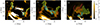 |
Fig. 6. Cuts across the volumetric emissivity along the z = 3 Mm (a), z = 4.5 Mm (b), and x = 13 Mm (c) plane corresponding to cuts across the coronal loop footpoints, coronal loop legs, and the coronal loop apex. The corresponding cuts across the individual waveguides are overplotted in blue (waveguide 1), green (waveguide 2), orange (waveguide 3), and red (waveguide 4). |
The boundary surfaces of the waveguides are complex and contain multiple folds that are aligned with the direction of the magnetic field strength. We quantified the complexity of the surface of each individual waveguide by calculating a circularity index Ic at different positions in the simulation domain: in the x = 13 Mm plane close to the apex of the magnetic loops in the simulation domain, in the z = 3 Mm plane close to the loop footpoints in the transition region, and in the z = 4.5 Mm plane intersecting the loop legs in the lower corona (the waveguide cross-sections are shown in Fig. 6). The circularity index is defined as Ic = 4πA/d2, where A is the cross-sectional area of the waveguide, and d is the circumference of the waveguide cross-section. It is a measure of a departure of the waveguide cross-section from a circular cross-section (Ic = 1 for a perfect circle). The Ic values of both footpoints and the apex for each waveguide are listed in Table 1 and vary from 0.11–0.41. We find that Ic in general decreases with height, except for waveguide 3, and is highest at the footpoints, and decreases at the apex. The asymmetry varies between the left and right footpoints.
Waveguide properties.
We further estimated the projected width of the waveguides, that is, the total extent of each waveguide along the z-axis at x = 13 Mm, when considering the LOS-projection (Table 1). This enabled us to compare the waveguide extent to the apparent width of the coronal loops observed in LOS-integrated emission. They vary from 2.21 Mm to 4.42 Mm, as opposed to the apparent loop widths in emission, which are of the order of several hundred kilometers (the exact values are depend on the instrument and bandpass), meaning that large parts of the waveguides are unaccounted for in EUV observations.
We finally calculated the waveguide filling factor, that is, the fraction of the total waveguide volume that is filled by the emitting coronal plasma. To estimate this, we set 2.88 × 10⁻⁶ erg cm−3 s−1 sr−1 as the emissivity threshold, the exact value of which depends on the instrument (in our model, the typical emissivity value for the background quiet corona are around 1 − 2 × 10⁻⁶ erg cm−3 s−1 sr−1). Plasma with a higher volumetric Fe IX emissivity than the threshold is considered to be emitting and is shown in yellow in Fig. 7. The filling factor values for the waveguides 1–4 are shown in Table 1 and range from 0.09–0.44.
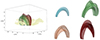 |
Fig. 7. Three-dimensional structure of waveguide 1 (blue), waveguide 2 (green), waveguide 3 (orange), and waveguide 4 (red). The volumetric emissivity above the threshold is shown in yellow. An animation of this figure is available online. |
4. Discussion
4.1. The coronal structure inferred from observations compared to self-consistent magnetohydrodynamics models
The convection-zone-to-corona models of the solar atmosphere seem to agree on the veil-like structure of the solar corona and the absence of well-defined cylindrical coronal loops, as also reported in Malanushenko et al. (2022).
Even in MHD models initiated with simple cylindrical loop configurations, it was found that the turbulent evolution of oscillating loops quickly leads to a distortion of the loop boundaries (Magyar & Van Doorsselaere 2018; Karampelas et al. 2019). This highlights that the models of coronal loops as long-lived confined structures might be too idealised in a real coronal environment. In a realistic corona that is highly dynamic and in which the coronal structures are subject to translational motion, oscillations in different modes and polarisations, and external perturbations leading to displacements of the magnetic structures (e.g. Kohutova & Popovas 2021; Kohutova et al. 2023), it is expected that they all affect the morphology and lifetimes of the coronal loops.
Additional complexities, such as the non-cospatiality of enhanced temperature and density structures, both of which lead to increased volumetric emissivity, have been highlighted in three-dimensional MHD simulations by Peter & Bingert (2012), Chen et al. (2014). Peter & Bingert (2012) also highlighted a case where a fraction of a simulated coronal loop was subject to temperature variations that were large enough to lie outside of the contribution function of the synthesised emission line. This coronal loop part hence appeared dark in the synthetic observations and might therefore lead to erroneous conclusions about the width, transverse density profile, and vertical cross-section variation in the coronal loop in question.
Observational analyses of the real cross-sectional structure of coronal loops remain limited. This is mainly due to the requirement of having multiple vantage points as well as sufficient spatial resolution to enable stereoscopic reconstruction, as a direct probing of the three-dimensional coronal structure is not possible. This has been attempted by McCarthy et al. (2021) using a combination of SDO/AIA and STEREO-EUVI (Kaiser et al. 2008) observations. They reported a lack of correlation between the loop diameters seen from multiple perspectives. This suggests features traditionally identified as monolithic and cylindrical coronal loops might in fact be more complex structures.
Using an alternative approach, Klimchuk & DeForest (2020) used Hi-C data to analyse the cross-sectional shape of the coronal loops by investigating the relation between the coronal loop width and the emission intensity seen in the EUV emission band centred on 193 Å. The lack of correlation between the coronal loop width and the intensity was used as a proof of circularity of the loop cross-section, under the key assumption that each coronal loop contains non-negligible magnetic twist. We note that an anti-correlation between the loop widths and intensity was found by McCarthy et al. (2021).
The discussion about whether coronal loops are better represented by confined strands or extended veils is nuanced, and very likely, both scenarios occur at some point in the corona. A notable example is a recently published analysis of the polarisation of a decayless kink oscillation using multi-viewpoint data from SDO/AIA and Solar Orbiter/EUI (Zhong et al. 2023), in which case the thin studied loop was well isolated from the surroundings and was identifiable in both datasets. However, conclusive observational evidence pointing to either form of the coronal structure being more prevalent is still lacking. A combination of newly available data from Solar Orbiter and SDO observations might shed more light on the question because of their potential for multi-viewpoint observations and the boost in the available resolution compared to stereoscopic studies using the pair of STEREO spacecraft. However, because of the stereoscopic ambiguity discussed by Malanushenko et al. (2022), the use of additional diagnostics might be necessary.
4.2. Concept of a waveguide
In the context of coronal oscillations, we typically understand by the term ‘waveguide’ or ‘wave cavity’ a coherent structure in the solar corona that can trap MHD waves and oscillates as a whole. It can guide propagating waves along and can undergo resonant, or standing-mode, oscillations, where the supported oscillation periods are one of the natural modes of the waveguide (e.g. Edwin & Roberts 1982, 1983), provided there is a sufficient change in the physical conditions inside and outside of the waveguide that cause wave refraction and act as a waveguide boundary (Nakariakov et al. 1996). In standard models of coronal oscillations, this boundary is typically provided by an increased density inside the loop, but a uniform density with a varying magnetic field strength is also possible (Howson et al. 2019). We based the waveguide identification on regions with high values of the magnitude of the Alfvén speed gradient, which act as a boundary for the magnetoacoustic waves. However, the exact behaviour of the waves at this boundary depends on the wave mode and frequency. Furthermore, we note that in a realistic coronal setup, both gravitational stratification and the magnetic field expansion cause the density and the magnetic field strength to vary along the magnetic field lines, leading to the variation in the Alfvén speed gradient along the magnetic field lines.
Our analysis suggests that in the self-consistent MHD models where the corona is driven by the dynamics of the lower solar atmosphere, the coronal waveguides are far from the idealised image of long and thin cylinders, and these approximations are therefore not valid in these models. In order to have a clear understanding of the coronal oscillations in this setup, it is necessary to model the oscillatory behaviour of the entire waveguide, including oscillation modes and their spatial characteristics and the oscillation polarisation. We further find that waveguide boundaries follow the veil-like features of the coronal structure, leading to a wrinkled waveguide surface. The waveguide cross-sections are far from circular, and the circularity index of the cross-sections decreases with the increasing height in the solar atmosphere. This might be caused by more complex dynamics higher in the simulated atmosphere, where small perturbations in chromospheric heights lead to larger disturbances in the corona because of the magnetic field expansion and density stratification.
We note that the emissivity structures are likely to vary on the timescales given by the sound speed, as they depend on density and temperature, whereas the spatial structure of the waveguides will vary on the Alfvén timescales. The mismatch between the two timescales adds another layer of complexity to the problem, and a detailed analysis of the temporal evolution of both structures is necessary to quantify this. The evolution of coronal oscillations and the temporal variation of the veil emissivity structure will be addressed in a follow-up work.
Our analysis highlights the complexity and a lack of clear one-to-one correspondence between a peak in the integrated emission profile that constitutes a loop cross-section, the regions of plasma along the LOS that contribute to this emission, and the regions of plasma that are bound by a large Alfvén speed gradient. This is clearly illustrated by waveguide 4, where what appears as two distinct loops D and E are in fact parts of a single waveguide with a large spatial extent.
Another factor that has to be considered when discussing waveguide characteristics is the waveguide skin depth. This corresponds to the exponential decay length at which the oscillation is evanescent at the boundary of the waveguide. Generally speaking, the skin depth also depends on oscillation mode and frequency. In the idealised scenario of a discontinuous boundary between a waveguide and the ambient plasma it is given by (Hindman & Jain 2021)
 (3)
(3)
Δ here corresponds to the length scale to which the oscillations extend beyond the waveguide, and is independent from the transverse geometry, ω is the frequency, kz is the longitudinal wavenumber, and ve is the Alfvén speed in the ambient plasma. We note that this is different from the ‘skin depth’ in some studies of coronal loop oscillations, where the term is simply used to refer to the width of the boundary layer in an idealised model of a cylindrical flux tube, where the density changes linearly from the internal (the coronal loop density) to the external value (ambient plasma density). This quantity is usually defined in the model setup a priori and is not directly related to the actual spatial extent of the wave field into the ambient plasma surrounding the waveguide.
The effect of the finite skin depth is that different waveguides located close to an oscillating waveguide will be affected when their separation is closer than the skin depth of that particular mode. This is the case in the coronal structures analysed in this work, as waveguides 1–4 lie very close to each other. The coupling of modes of an oscillating coronal loop to the modes of the surrounding arcade was investigated by Hindman & Jain (2021), highlighting the possibility of an arcade resonance that appears as resonant modes of individual loops and might lead to errors in the seismological estimates. Although the model is limited to 2D, a very similar coupling can be expected in three dimensions. Similarly, Luna et al. (2019) investigated oscillation modes of a cluster of strands and reported a large degree of collective behaviour.
The observational evidence also seems to suggest that coronal loops in an active region do not oscillate in isolation, but are often coupled to oscillations of surrounding structures (Verwichte et al. 2004, 2009; Jain et al. 2015; Tian et al. 2016; Li et al. 2023). The nature of the EUV observations means, however, that only the evolution of the emitting loops can be analysed.
This suggests that the connection of the coronal waveguides to the ambient plasma should be also considered, as opposed to modelling coronal loops as isolated entities. The downside is the complexity of modelling the collective oscillation of the whole active region loop system. This is not to say that well-defined coronal loops evolving independently of their surroundings do not exist. For instance, loops that catastrophically cool and exhibit coronal rain, considered to be in a state of thermal non-equilibrium and thermal instability (known as ‘TNE-TI’ scenario Antolin & Froment 2022), can be considered as isolated coronal waveguides, and Şahin & Antolin (2022) showed that they can be prevalent over an active region.
In the above analysis we have also estimated the waveguide filling factors, that is, the fraction of the coronal waveguide that is filled with plasma that emits in EUV. We note that the exact values will depend on the resolution and the sensitivity of the instrument, as well as on the wavelength extent of the instrument bandpass. The overarching conclusion that is still valid regardless of the above is that we can only observe a small part of the actual coronal waveguide. The discussion of the filling factors in the corona is usually focused on the volume filling factors of multistranded coronal loops, to quantify the number of strands that emit in the given channel (Peter et al. 2013), where the outer envelope of the loop is determined from EUV observations. In our work, we focused on the relation between the EUV volumetric emissivity and regions that are bounded by large Alfvén speed gradients.
The natural next step is to investigate the link between the temporal evolution and oscillations in the EUV emission and the actual dynamics of the oscillating plasma structures in three dimensions; this will be done in a follow-up study. The impact of these non-ideal waveguides on the accuracy of the coronal seismology will also be addressed.
4.3. Model limitations
One of the obvious limitations of the model we used (and by extension, of most purely MHD codes that are used to simulate the solar atmosphere with high realism) is the artificially low Reynolds number. This affects the formation of the fine-scale structure in the model because the code is inherently diffusive. Despite this, the observed fine-scale structure of the corona, as it appears in LOS-integrated emission, is still reproduced (Malanushenko et al. 2022). The fine-scale structure is additionally affected by the spatial resolution of the model.
The coronal structure reproduced in convection-zone-to-corona simulations might simply be an artefact of the model. However, the fact that the same veil structure has been reported in self-consistent MURaM simulations suggests that this structure of the corona is independent of the model. Furthermore, even models that only include a coronal waveguide are also subject to strong LOS superposition, which leads to the apparent strand formation (Antolin et al. 2014). The properties of coronal oscillations that are reproduced in these models such as the excitation of different modes, harmonics, and the oscillation damping timescales, so far agree with the observations (Kohutova & Popovas 2021; Kohutova et al. 2023). More generally, a number of complex phenomena has been successfully reproduced by the convection-zone-to-corona models including solar flares (Cheung et al. 2019), surges (Nóbrega-Siverio et al. 2016), the formation of coronal rain (Kohutova et al. 2020), and coronal bright points (Nóbrega-Siverio et al. 2023), all suggesting a high degree of realism of the solar atmosphere in these models.
Regardless of how accurate the solar corona that forms in convection-zone-to-corona models really is, we highlighted the possibility that observations of oscillations in coronal structures might be misinterpreted, namely of what does constitute a waveguide. This can occur as a result of the ambiguities induced by the LOS integration combined with the finite temperature-range sensitivity of a given bandpass and the fact that both the density and the magnetic structure govern the propagation and potentially also the trapping of MHD waves in the corona.
5. Conclusions
We have extended the implications of the coronal veil model of the solar corona to models of coronal oscillations. Using the convection-zone-to-corona simulations with the radiation-MHD code Bifrost, we analysed the structure of the simulated corona that forms self-consistently in the model. We conclude that the coronal veil structure is independent of the model and appears in convection-zone-to-corona models other than MURaM.
We focused on the spatial variability of the volumetric emissivity of the Fe IX 171.073 Å EUV line and on the variability of the Alfvén speed, which captures the density and magnetic structuring of the simulated corona. We traced features with boundaries associated with the large magnitudes of the Alfvén speed gradient and which most likely trap MHD waves and act as coronal waveguides. We also searched for the correspondence with emitting regions that appear as strand-like loops in LOS-integrated EUV emission.
We found that the cross-sections of the waveguides bounded by large Alfvén speed gradients become less circular and more distorted with increasing height in the solar atmosphere. Small filling factors corresponding to the fraction of the waveguides filled with plasma that emits in the given EUV wavelength suggest that we can only observe a small fraction of the waveguide. Similarly, the projected waveguide widths in the plane of the sky are several times larger than the widths of the apparent loops that can be observed in EUV. Our results point to the lack of a straightforward correspondence between a peak in the integrated emission profile that constitutes an apparent coronal loop and regions of plasma that are bound by a large Alfvén speed gradient acting as waveguides. This may lead to incorrect assumptions about the size, shape, and transverse density structuring of the oscillating coronal features. Coronal waveguides therefore cannot be idientified reliably based on emission in a single EUV wavelength in the simulated corona that forms in convection-zone-to-corona models.
Data availability
Movies associated to Figs 3, 4, and 7 are available at https://www.aanda.org
Acknowledgments
PK and NP acknowledge funding from the Research Council of Norway, project no. 324523. This research was also supported by the Research Council of Norway through its Centres of Excellence scheme, project no. 262622 and through grants of computing time from the Programme for Supercomputing.
References
- Antolin, P., & Froment, C. 2022, Front. Astron. Space Sci., 9, 820116 [NASA ADS] [CrossRef] [Google Scholar]
- Antolin, P., & Rouppe van der Voort, L. 2012, ApJ, 745, 152 [Google Scholar]
- Antolin, P., Yokoyama, T., & Van Doorsselaere, T. 2014, ApJ, 787, L22 [Google Scholar]
- Antolin, P., Dolliou, A., Auchère, F., et al. 2023, A&A, 676, A112 [NASA ADS] [CrossRef] [EDP Sciences] [Google Scholar]
- Berghmans, D., Antolin, P., Auchère, F., et al. 2023, A&A, 675, A110 [NASA ADS] [CrossRef] [EDP Sciences] [Google Scholar]
- Chen, F., Peter, H., Bingert, S., & Cheung, M. C. M. 2014, A&A, 564, A12 [NASA ADS] [CrossRef] [EDP Sciences] [Google Scholar]
- Cheung, M. C. M., Rempel, M., Chintzoglou, G., et al. 2019, Nat. Astron., 3, 160 [NASA ADS] [CrossRef] [Google Scholar]
- Del Zanna, G., Dere, K. P., Young, P. R., & Landi, E. 2021, ApJ, 909, 38 [NASA ADS] [CrossRef] [Google Scholar]
- Edwin, P. M., & Roberts, B. 1982, Sol. Phys., 76, 239 [Google Scholar]
- Edwin, P. M., & Roberts, B. 1983, Sol. Phys., 88, 179 [Google Scholar]
- Gudiksen, B. V., Carlsson, M., Hansteen, V. H., et al. 2011, A&A, 531, A154 [NASA ADS] [CrossRef] [EDP Sciences] [Google Scholar]
- Hindman, B. W., & Jain, R. 2021, ApJ, 921, 29 [CrossRef] [Google Scholar]
- Howson, T. A., De Moortel, I., Antolin, P., Van Doorsselaere, T., & Wright, A. N. 2019, A&A, 631, A105 [NASA ADS] [CrossRef] [EDP Sciences] [Google Scholar]
- Jain, R., Maurya, R. A., & Hindman, B. W. 2015, ApJ, 804, L19 [NASA ADS] [CrossRef] [Google Scholar]
- Kaiser, M. L., Kucera, T. A., Davila, J. M., et al. 2008, Space Sci. Rev., 136, 5 [Google Scholar]
- Karampelas, K., Van Doorsselaere, T., & Guo, M. 2019, A&A, 623, A53 [NASA ADS] [CrossRef] [EDP Sciences] [Google Scholar]
- Klimchuk, J. A., & DeForest, C. E. 2020, ApJ, 900, 167 [NASA ADS] [CrossRef] [Google Scholar]
- Kohutova, P., & Popovas, A. 2021, A&A, 647, A81 [NASA ADS] [CrossRef] [EDP Sciences] [Google Scholar]
- Kohutova, P., & Verwichte, E. 2016, ApJ, 827, 39 [CrossRef] [Google Scholar]
- Kohutova, P., Antolin, P., Popovas, A., Szydlarski, M., & Hansteen, V. H. 2020, A&A, 639, A20 [EDP Sciences] [Google Scholar]
- Kohutova, P., Antolin, P., Szydlarski, M., & Carlsson, M. 2023, A&A, 676, A32 [NASA ADS] [CrossRef] [EDP Sciences] [Google Scholar]
- Li, D., Bai, X., Tian, H., et al. 2023, A&A, 675, A169 [NASA ADS] [CrossRef] [EDP Sciences] [Google Scholar]
- Luna, M., Oliver, R., Antolin, P., & Arregui, I. 2019, A&A, 629, A20 [NASA ADS] [CrossRef] [EDP Sciences] [Google Scholar]
- Magyar, N., & Van Doorsselaere, T. 2018, ApJ, 856, 144 [Google Scholar]
- Malanushenko, A., Cheung, M. C. M., DeForest, C. E., Klimchuk, J. A., & Rempel, M. 2022, ApJ, 927, 1 [NASA ADS] [CrossRef] [Google Scholar]
- McCarthy, M. I., Longcope, D. W., & Malanushenko, A. 2021, ApJ, 913, 56 [NASA ADS] [CrossRef] [Google Scholar]
- Nakariakov, V. M., & Kolotkov, D. Y. 2020, ARA&A, 58, 441 [Google Scholar]
- Nakariakov, V. M., Roberts, B., & Mann, G. 1996, A&A, 311, 311 [NASA ADS] [Google Scholar]
- Nóbrega-Siverio, D., Moreno-Insertis, F., & Martínez-Sykora, J. 2016, ApJ, 822, 18 [Google Scholar]
- Nóbrega-Siverio, D., Moreno-Insertis, F., Galsgaard, K., et al. 2023, ApJ, 958, L38 [CrossRef] [Google Scholar]
- Peter, H., & Bingert, S. 2012, A&A, 548, A1 [NASA ADS] [CrossRef] [EDP Sciences] [Google Scholar]
- Peter, H., Bingert, S., Klimchuk, J. A., et al. 2013, A&A, 556, A104 [NASA ADS] [CrossRef] [EDP Sciences] [Google Scholar]
- Reale, F. 2014, Living Rev. Sol. Phys., 11, 4 [NASA ADS] [CrossRef] [Google Scholar]
- Şahin, S., & Antolin, P. 2022, ApJ, 931, L27 [CrossRef] [Google Scholar]
- Scullion, E., Rouppe van der Voort, L., Wedemeyer, S., & Antolin, P. 2014, ApJ, 797, 36 [Google Scholar]
- Stein, R. F., Nordlund, Å., Collet, R., & Trampedach, R. 2024, ApJ, 970, 24 [NASA ADS] [CrossRef] [Google Scholar]
- Tian, H., Young, P. R., Reeves, K. K., et al. 2016, ApJ, 823, L16 [Google Scholar]
- Verwichte, E., Nakariakov, V. M., Ofman, L., & Deluca, E. E. 2004, Sol. Phys., 223, 77 [Google Scholar]
- Verwichte, E., Aschwanden, M. J., Doorsselaere, T. V., Foullon, C., & Nakariakov, V. M. 2009, ApJ, 698, 397 [NASA ADS] [CrossRef] [Google Scholar]
- Williams, T., Walsh, R. W., Winebarger, A. R., et al. 2020, ApJ, 892, 134 [Google Scholar]
- Zhong, S., Nakariakov, V. M., Kolotkov, D. Y., et al. 2023, Nat. Commun., 14, 5298 [NASA ADS] [CrossRef] [Google Scholar]
All Tables
All Figures
|
Fig. 1. Coronal structure in the simulation. We show the LOS-integrated Fe IX emission intensity in the x–z plane (a). The dashed line at x = 13 Mm marks the y–z plane along which the subsequent slices are taken. The dotted lines mark a portion of the loop axis for loops A–E. Vertical slices taken across the coronal loops at x = 13 Mm show the plasma temperature (b), volumetric emissivity (c), and the plasma density (d). |
| In the text | |
|
Fig. 2. Vertical slice across the volumetric emissivity at x = 13 Mm (right), and the corresponding x = 13 Mm LOS-integrated emission profile (left). The local emission peaks corresponding to the loops A–E are marked by dashed purple lines. These also mark the z-coordinates of the contributing regions in the emissivity slice. The dominant emitting regions corresponding to each loop are marked by purple rectangles. |
| In the text | |
|
Fig. 3. Three-dimensional rendering of |∇vA| (a) and the volumetric emissivity ϵFe IX (b). An animation is available online. |
| In the text | |
|
Fig. 4. Horizontal slices across |∇vA| at z = 2 Mm (a) z = 5 Mm (b) and z = 10 Mm (c). An animation is available online. |
| In the text | |
|
Fig. 5. x = 13 Mm slice across |∇vA|. The cross sections of waveguides encompassing dominant emitting regions for each loop are shown in blue (waveguide 1), green (waveguide 2), orange (waveguide 3), and red (waveguide 4). The emissivity contours are overplotted. |
| In the text | |
|
Fig. 6. Cuts across the volumetric emissivity along the z = 3 Mm (a), z = 4.5 Mm (b), and x = 13 Mm (c) plane corresponding to cuts across the coronal loop footpoints, coronal loop legs, and the coronal loop apex. The corresponding cuts across the individual waveguides are overplotted in blue (waveguide 1), green (waveguide 2), orange (waveguide 3), and red (waveguide 4). |
| In the text | |
|
Fig. 7. Three-dimensional structure of waveguide 1 (blue), waveguide 2 (green), waveguide 3 (orange), and waveguide 4 (red). The volumetric emissivity above the threshold is shown in yellow. An animation of this figure is available online. |
| In the text | |
Current usage metrics show cumulative count of Article Views (full-text article views including HTML views, PDF and ePub downloads, according to the available data) and Abstracts Views on Vision4Press platform.
Data correspond to usage on the plateform after 2015. The current usage metrics is available 48-96 hours after online publication and is updated daily on week days.
Initial download of the metrics may take a while.