| Issue |
A&A
Volume 689, September 2024
|
|
|---|---|---|
| Article Number | A295 | |
| Number of page(s) | 12 | |
| Section | The Sun and the Heliosphere | |
| DOI | https://doi.org/10.1051/0004-6361/202449677 | |
| Published online | 19 September 2024 | |
Effects of coronal rain on decayless kink oscillations of coronal loops⋆
1
Aryabhatta Research Institute of Observational Sciences, Nainital 263002, India
e-mail: This email address is being protected from spambots. You need JavaScript enabled to view it.
2
Indian Institute of Astrophysics, Bangalore 560034, India
3
Joint Astronomy Programme and Department of Physics, Indian Institute of Science, Bangalore 560012, India
4
Department of Mathematics, Physics and Electrical Engineering, Northumbria University, Newcastle Upon Tyne NE1 8ST, UK
Received:
20
February
2024
Accepted:
11
May
2024
Abstract
Decayless kink oscillations are ubiquitously observed in active region coronal loops with an almost constant amplitude for several cycles. Decayless kink oscillations of coronal loops triggered by coronal rain have been analyzed, but the impact of coronal rain formation in an already oscillating loop is unclear. As kink oscillations can help diagnose the local plasma conditions, it is important to understand how these are affected by coronal rain phenomena. In this study, we present the analysis of an event of coronal rain that occurred on 25 April 2014 and was simultaneously observed by Slit-Jaw Imager (SJI) on board Interface Region Imaging Spectrograph (IRIS) and Atmospheric Imaging Assembly (AIA) on board the Solar Dynamic Observatory (SDO). We investigated the oscillation properties of the coronal loop in AIA images before and after the appearance of coronal rain as observed by SJI. We find signatures of decayless oscillations before and after coronal rain at similar positions to those found during coronal rain. The individual cases show a greater amplitude and period during coronal rain. The mean period is increased by 1.3 times during coronal rain, while the average amplitude is increased by 2 times during rain, in agreement with the expected density increase from coronal rain. The existence of the oscillations in the same loop at the time of no coronal rain indicates the presence of a footpoint driver. The properties of the observed oscillations during coronal rain can result from the combined contribution of coronal rain and a footpoint driver. The oscillation amplitude associated with coronal rain is approximated to be 0.14 Mm. The properties of decayless oscillations are considerably affected by coronal rain, and without prior knowledge of coronal rain in the loop, a significant discrepancy can arise from coronal seismology with respect to the true values.
Key words: Sun: corona / Sun: oscillations
Movie associated to Fig. 1 is available at https://www.aanda.org.
© The Authors 2024
 Open Access article, published by EDP Sciences, under the terms of the Creative Commons Attribution License (https://creativecommons.org/licenses/by/4.0), which permits unrestricted use, distribution, and reproduction in any medium, provided the original work is properly cited.
This article is published in open access under the Subscribe to Open model. This email address is being protected from spambots. You need JavaScript enabled to view it. to support open access publication.
1. Introduction
Coronal loops are building blocks of the solar corona, and the dense, confined plasma that constitutes them gives rise to their brightness (Reale 2010). Non-thermal velocities and up-flows have been observed near footpoints of active region coronal loops, suggesting footpoint heating (Doschek et al. 2007; Hara et al. 2008). Thermal conduction distributes the footpoint heating to the chromosphere, which heats the plasma, leading to chromospheric evaporation. The density increases in the corona, which eventually becomes thermally imbalanced, with radiative cooling dominating the heating, and driving the loop into a state of thermal nonequilibrium (TNE) cycle, which is a global state of a coronal loop (for a detailed review of the TNE cycle, we refer the reader to Antolin 2020; Antolin & Froment 2022). During cooling, thermal instability (TI) can set in at a specific density and temperature value. Because of this process, the loop apex cools down catastrophically to chromospheric and transition-region temperatures, forming plasma clumps within a few minutes. These clumps fall along the loop, guided by the magnetic field lines, and are known collectively as coronal rain. The first reports of coronal rain date back to the 1970s (Kawaguchi 1970; Leroy 1972), although McMath & Pettit (1938) provide the first description of a phenomenon that strongly resembles coronal rain. When seen on the limb, the coronal rain clumps appear as bright features in the chromospheric lines, such as Hα (De Groof et al. 2004, 2005) and Ca II H (Antolin et al. 2010; Antolin & Verwichte 2011), or transition region lines, such as He II and Si IV (De Groof et al. 2005; Antolin et al. 2015). These clumps appear as dark structures when observed on-disk (Antolin et al. 2012). They fall towards the solar surface with acceleration of less than the free-fall gravitational acceleration, and numerical simulations indicate an increased pressure gradient downstream of the rain as one of the reasons for this difference (Müller et al. 2004; Antolin et al. 2010; Oliver et al. 2014). Coronal rain has previously been considered a sporadic phenomenon with a frequency in days (Schrijver 2001), but more recent estimates of occurrence times using high-resolution observations with the Swedish 1 m Solar Telescope show that coronal rain is a common phenomenon of active regions (Antolin & Rouppe van der Voort 2012). More recently, a strong link was established between coronal rain and the phenomenon of long-period intensity pulsations (Auchère et al. 2018). The latter corresponds to highly periodic extreme-ultraviolet (EUV) pulsations observed along coherent structures (such as loops) lasting several days (Auchère et al. 2014; Froment et al. 2015), now understood as the manifestation of TNE cycles in loops (Froment et al. 2017, 2018; Pelouze et al. 2022). Coronal rain can therefore be recurrent in the same loop bundle over a timescale of hours. The density of coronal rain clumps varies within the range of 1010 − 1012 cm−3 (Antolin et al. 2015) and, on average, these clumps have widths of hundreds of kilometers (km) and lengths reaching up to a few thousand km. The formation of coronal rain carries important observable features in the EUV. As the rain forms, magnetically enhanced strands strongly emitting in the UV and EUV can form due to flux freezing, and are linked to the condensation-corona transition region (CCTR) at the boundaries of the rain. Furthermore, significant compression can occur downstream from the rain, leading to strongly variable plume-like structures (Antolin et al. 2022).
Coronal loop oscillations are powerful tools for diagnosing coronal parameters through magnetohydrodynamic (MHD) seismology. Transverse oscillations in coronal loops have been interpreted as fast MHD kink waves (Edwin & Roberts 1983; Roberts et al. 1984). The Transition Region and Coronal Explorer (TRACE) observed the earliest transverse oscillations of coronal loops in EUV wavelengths (Aschwanden et al. 1999; Schrijver et al. 1999; Nakariakov et al. 1999). Coronal rain, prominences, and similar chromospheric flows occurring in the corona have also been used as tracers of transverse MHD waves (Okamoto et al. 2007; Ofman & Wang 2008; Antolin & Verwichte 2011; Kohutova & Verwichte 2016; Verwichte et al. 2017; Verwichte & Kohutova 2017). Furthermore, ultra-long period oscillations (10−30 h), interpreted in terms of MHD waves, have been observed in filaments (Foullon et al. 2004, 2009). The first identification of transverse oscillations in coronal rain was performed by Antolin & Verwichte (2011) using the Hinode/Solar Optical Telescope. These oscillations have amplitudes of below 500 km and periods in the range of 100−200 s. The oscillations were interpreted as the first harmonic of the standing kink MHD mode because the amplitude of oscillations was maximum at midway between the loop apex and footpoint. Coronal loops have been seen to exhibit persistent low-amplitude oscillations, known as decayless kink oscillations, that show no apparent decay over multiple periods. These latter are frequent features in the solar corona (Anfinogentov et al. 2015; Gao et al. 2022; Shrivastav et al. 2024). The study of Kohutova & Verwichte (2016) revealed low-amplitude, persistent transverse oscillations of coronal rain with an average period of 3.4 min and amplitude lying between 0.2 and 0.4 Mm.
Verwichte & Kohutova (2017) reported the first observation of the excitation of kink oscillations by coronal rain. This study indicated that the oscillations become apparent as condensation forms due to the significant coronal rain mass. Kohutova & Verwichte (2017) performed a 2.5 dimensional numerical MHD simulation of a coronal loop by introducing low-temperature, highly condensed mass at the loop top. The loop was displaced downwards, setting up the transverse oscillation. This latter study shows that the amplitude of the excited transverse oscillations increases with rain mass compared to the total loop mass. This study also revealed that as the rain blobs fall towards the loop leg, the period of kink oscillations decreases due to the temporally varying average density of the loop. The generation of transverse MHD waves by coronal rain was first studied analytically by Verwichte et al. (2017). These authors present a mechanical model of coronal rain, which they used to investigate the role of the ponderomotive force arising from the transverse oscillations in the kinematics of rain blobs. The authors find that the low amplitudes of transverse oscillations previously seen in rain events are insufficient to account for the reduced downward acceleration. The model indicates that the amplitude of excited transverse oscillations due to the rain is likely to depend on various parameters and to be affected by the timescales of rain formation. Although kink oscillations and coronal rain are common phenomena in active region loops, the cause-and-effect relationship is unclear. For instance, although coronal rain can excite transverse MHD oscillations, it is not clear how common this process is in the solar corona. We present observations of transverse oscillations accompanied by coronal rain and simultaneously observed by the Slit-Jaw Imager (SJI) and Atmospheric Imaging Assembly (AIA). We applied the motion magnification technique to magnify transverse oscillations in the AIA channels, which allowed us to detect and compare the properties of oscillations before, during, and after coronal rain.
The paper is arranged as follows: Section 2 covers the details of the observations and data. In Sect. 3, we present the methodology, individual cases of oscillations before and after coronal rain, and a comparison of the average properties of oscillations. In Sect. 4, we summarise the work and discuss the possible scenarios leading to the observed results.
2. Observational data
We studied coronal rain observed by SJI on board IRIS (De Pontieu et al. 2014) at the northeast limb on April 25, 2014. IRIS started observing the region around 00:39 UT and observed the event in two passbands, 1400 (far-UV) and 2796 (near-UV). The emission in the SJI 1400 passband is contributed by Si IV emission lines that form at the transition region temperature of about 63 000 K, whereas the SJI 2796 passband is dominated by the Mg II K line core that forms at the chromospheric temperature of about 10 000 K. The dataset has a pixel scale of 0.166″ pix−1 and a cadence of 18.7 s. IRIS observations are centered around [x, y]=[957″, 229″].
The event was also observed by AIA (Lemen et al. 2012) on board SDO (Pesnell et al. 2012), which provides full-disk, nearly simultaneous observations of the Sun in seven EUV narrow-band filters, and has a pixel-scale of 0.6″ pix−1 and a cadence of 12 s. AIA data are derotated, co-aligned, and brought to the same pixel scale using aia_prep.pro. Coronal rain condensations are spotted in AIA 304 channel, which is dominated by He II (304 Å) emission at approximately equal to 50 000 K. Of all the AIA channels, the loop system was best visible in the AIA 171 passband (dominated by Fe IX 171.09 Å emission at 0.7 MK). We therefore used 304 and 171 passband images to analyze this event.
Figure 1a shows the AIA 171 intensity image processed using the multi-Gaussian normalization (MGN) technique (Morgan & Druckmüller 2014) at 03:15 UT. The green rectangle represents the field of view (FOV) observed by SJI, and Fig. 1b shows a zoomed-in view of the same FOV with the loop system observed in AIA 171. Panels c–e in Fig. 1 show the coronal rain in SJI 1400, 2796, and AIA 304, respectively. A radial gradient filter similar to a normalizing radial graded filter (Morgan et al. 2006) is applied to SJI 2796, 1400, and AIA 304 intensity images to enhance off-limb intensity. AIA 171 intensity images appear fuzzy due to the diffuse background and foreground emission (DelZanna & Mason 2003; Viall & Klimchuk 2013) produced in an active-region coronal loop system with a peak temperature of about 1.5 MK (Subramanian et al. 2014; Brooks 2019). Although it is difficult to segregate adjacent loops and their strands, we attempt to separate the loops with diffuse emission using unsharp masking to identify oscillating strands, as shown in Fig. 2b. The images are convolved with a Gaussian kernel to remove the noise and are then subtracted from the original to identify and enhance the edges. AIA and SJI channels are aligned by matching the off-limb features in the near-simultaneous images of SJI 1400 and AIA 304.
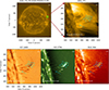 |
Fig. 1. Overview of the observation. (a) Full-disk intensity image of the Sun in AIA 171 processed using the MGN technique. The small green box highlights the event location and FOV of SJI. (b) Zoomed-in view of the green box in AIA 171 Å with the loop system. (c)–(e) Approximately simultaneous SJI 1400, 2796, and AIA 304 (radial-gradient-filtered) images. The presence of coronal rain in the loops can be seen. The cyan lines mark the position of artificial slits chosen for generating space-time maps. Slit 8 overlaps the position of a smaller loop. An animation associated with this figure is available online. |
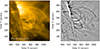 |
Fig. 2. Example of edge detection in AIA 171 images. The left panel shows the AIA 171 intensity image of the small green box shown in Fig. 1. The fuzziness of the emission is clearly visible. The right panel shows the unsharp masked inverted image of the same FOV in which loop edges are enhanced. |
Additionally, we used data from the Extreme Ultraviolet Imager (EUVI; Wuelser et al. 2004) on board the Solar Terrestrial Relations Observatory (STEREO; Kaiser et al. 2008). The EUVI captures full-disk images of the Sun in four passbands, with a pixel scale of 1.6″ pix−1. For our analysis, we relied on the 171 Å images to estimate the 3D geometry of the loop. During the observation period, EUVI 171 provided only two images.
3. Analysis and results
3.1. Space-time maps
We placed eight artificial slits over two coronal loops at different positions to capture oscillations before, during, and after coronal rain. Figures 1b–e show the positions of the slits as cyan lines orthogonal to the loop in different passbands. Slits 1 to 7 are placed on the larger loop, while the second loop hosting slit 8 is smaller. These artificial slits are five pixels wide, and intensity is averaged across the artificial slit to increase the signal-to-noise ratio (S/N). Figure 3a shows the space-time (x − t) maps for slit 1 in SJI 1400, and it is evident that different blobs are subjected to transverse oscillations. These x − t maps also indicate that these oscillations are decayless, and we did not observe any eruption or flare near the loop system for about 3 h before the start of IRIS observation. It is important to highlight that the rain blobs observed between 02:50 and 02:56 UT in Fig. 3a are oscillating in phase, indicating the potential existence of standing kink oscillations.
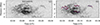 |
Fig. 3. Oscillation detection and fitting. (a) Space-time map of Slit 1 near the apex of the loops in SJI 1400 are shown in Fig. 1. The negative intensity is shown in each map. These x − t maps show that the different rain clumps oscillate in phase at varying positions of the slits. The decay-less nature of transverse oscillations is also visible in the x − t maps. (b) The plus symbols mark the centers of the threads over-plotted with the obtained sinusoidal fits, which are represented by red curves. The oscillation properties are derived using sinusoidal fits. |
To determine oscillation parameters, we estimated the oscillating thread center by fitting a Gaussian function over the distance along the slit at each time step. The centers of best-fit Gaussian are overplotted with a “plus” symbol over time distance maps (see Fig. 3b). We fitted the oscillations using the following relation:
 (1)
(1)
where A0 is the mean position, A1 is displacement amplitude, P is time period, ϕ is the phase, A2 is a constant parameter for linear trend, k is a coefficient for the linear increase or decrease in the period of oscillations, and τ provides the damping or growth timescale. We used the Levenberg-Marquardt least-squares minimization to obtain fitting parameters. The obtained fits for slit 1 are plotted with the centers in Fig. 3b. We use the width of the fitted Gaussian as the uncertainty on the position of the loop. The amplitude and period are also supplemented with errors obtained after sinusoidal fitting. The parameters of the fitted oscillations are provided in Table A.1.
3.2. Motion magnification
We find oscillations with an average amplitude of less than 1 Mm in SJI 1400 and 2796 x − t maps. It was challenging to find oscillations at the same spatial positions in AIA channels as these amplitudes are comparable to the pixel resolution of AIA. Anfinogentov et al. (2015) showed that low-amplitude decayless oscillations are common features in solar corona, with an average displacement amplitude of less than the pixel size of AIA. To enhance the transverse motions in AIA observations, we used the motion magnification (Anfinogentov & Nakariakov 2016) technique, which magnifies transverse oscillation amplitudes while preserving the oscillation periods. This technique was previously used for the identification of second harmonics of decayless kink oscillations (Duckenfield et al. 2018), coronal seismology of quiet Sun using decayless kink oscillations (Anfinogentov & Nakariakov 2019), investigation of transverse oscillations linked to flares (Mandal et al. 2021), and identification of decayless oscillations in coronal bright points (Gao et al. 2022). In this work, we use a magnification factor of 7 as we find this to be optimal for identifying the oscillations.
3.3. Individual cases of oscillations before and after coronal rain
3.3.1. Oscillations in the smaller loop
We used the motion magnification algorithm to capture oscillations before and after coronal rain. Figure 4a shows x − t maps – generated after motion magnification – corresponding to slit 8 on the smaller loop in AIA 171. The x − t maps are presented in inverted intensity, and so dark features correspond to emission. The two blue vertical lines in Fig. 4a correspond to the time of the start and end of the coronal rain, as observed from SJI 2796. The SJI 2796 x − t map shows the signature of oscillations between 4 and 6 Mm. The oscillation observed in slit 8 in Fig. 4b shows the increase in amplitude over time. We fitted this growing amplitude oscillation using Eq. (1) in Wang et al. (2012), which is overplotted in red. The oscillation amplitude and period are computed as 0.11 ± 0.01 Mm and 2.1 ± 0.01 min, respectively. The growth timescale, tg, for oscillation is 695 s. The increase in the amplitude is estimated from the ratio A1, t1/A1, t0 = e(t1 − t0)/tg = 2.1, where t0 and t1 are the start and end time of the observed oscillation. If we trace back to a similar location in the AIA 171 passband in Fig. 4a, we see an oscillation, O1, between 02:35 and 02:41 UT with an amplitude of 0.09 ± 0.01 Mm and a period of 1.7 ± 0.04 min. We confirm the presence of oscillation signatures around 03:12 UT (i.e., during the coronal rain) in the AIA 304 channel between 4 and 6 Mm. The oscillating blob is not fitted for AIA 304 because it does not have a clear contrast relative to the background. During coronal rain, we detect the oscillation labeled as O2 in emission from 5 to 7 Mm in the AIA 171 x − t map. This could be a signature of coronal rain oscillation in CCTR emission.
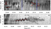 |
Fig. 4. Oscillations captured in smaller loop. (a) AIA 171 x − t map of Slit 8 for the time before, during, and after coronal rain. The blue vertical lines indicate the time interval when coronal rain was present in the SJI 2796 passband. The x − t maps for AIA channels are produced after motion magnification. These x − t maps are inverted in intensity. (b) The x − t map of Slit 8 in SJI 2796. The increase in amplitude is clearly visible, and the oscillation is fitted with the red curve. |
The coronal rain is observed in SJI 2796 between 03:02 and 03:24 UT. Just after 03:24 UT, we see an oscillation, O3, at about 4 Mm in AIA 171. The estimated amplitude and period are 0.07 ± 0.01 Mm and 1.9 ± 0.02 min, respectively. We do not see a clear signature of oscillations after 03:30 UT in AIA 171. The diffused background and foreground and overlapping loops can make it challenging to capture oscillations after motion magnification. The increase or decrease in emission in a particular passband due to the thermal evolution of the loop top could also be the cause of the fading nature of these oscillations. The thermal evolution for the loop top is not discussed for the smaller loop, as the emission in cooler channels was affected by coronal rain in a foreground loop.
3.3.2. Oscillations in the larger loop
Figures 5a–c display the location of the curved slit in AIA 304, SJI 2796, and AIA 171 intensity images taken along the larger loop. Panels d–f in Fig. 5 depict the corresponding x − t maps for the curved slit, with the black dashed line indicating the location of slit 3 on the curved slit. Rain blob signatures are observed near the loop top in AIA 304 and SJI 2796 x − t maps after 02:55 UT. These maps reveal the position of rain blobs along the loop, reaching the bottom of the loop around 03:25 UT. Notably, there is no evidence of rain in the loop between 02:27 and 02:55 UT, as observed in AIA 304 and SJI 2796 x − t maps. This suggests that rain occurred only between 02:55 and 03:25 in the larger loop. The AIA 171 x − t map shows the coronal rain signature in EUV absorption around 03:20 UT, indicated by the dashed red line (see Fig. 5f). The line is shifted in the time axis to view the rain in absorption clearly. The corresponding positions of the red line in AIA 304 and SJI 2796 are indicated by blue lines.
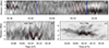 |
Fig. 5. Tracking of the rain blobs along larger loop. Panels a–c depict the location of the curved slit traced along the rain blobs in AIA 304, SJI 2796, and along the loop in AIA 171. Here we aim aim to detect the presence of rain blobs. The placement of the slit is determined based on the trajectory of the rain blobs observed in SJI 2796 images. Panels d–f illustrate the x − t maps associated with the curved slit in AIA 304, SJI 2796, and AIA 171. The black line in the x − t maps represents the estimated position of slit 3 on the curved slit. Around 03:20 UT, the descending rain in EUV absorption is traced by the red dashed line in the AIA 171 x − t map. The line is displayed with an offset to clearly identify the rain features in EUV absorption. The blue dashed line in AIA 304 and SJI 2796 corresponds to the red dashed line in AIA 171. |
Figures 6a–c show the x − t maps for slit 3 on the bigger loop in which the x − t maps of AIA 171 and 304 are made after motion magnification. AIA 171 x − t map of slit 3 shows the detected oscillation, O1, around 02:30 UT, while the coronal rain started after 02:55 UT. The oscillation has amplitude and period of 0.08 ± 0.02 Mm and 2.6 ± 0.02 min, respectively. The oscillation captured by AIA 304 has amplitude and period of 0.16 ± 0.01 Mm and 3.8 ± 0.09 min, respectively, though these values are 0.22 ± 0.04 Mm and 3.9 ± 0.03 min for the oscillation captured by SJI 2796. However, when we plot the oscillations detected in slit 3 using SJI 2796 and AIA 304 channels on the same time line and position along the slit, we find that they line up and have similar phases (see Fig. 7). Furthermore, their mean positions along the slit are close to each other, suggesting that these oscillations are almost identical. The oscillations during coronal rain are seen in AIA 304, and SJI 2796 persisted until 03:17 UT (Figs. 6b and c). We find evidence of oscillations at similar positions in AIA 171 x − t maps after coronal rain in different slits. Figure 6a shows the oscillation, O4, in the AIA 171 x − t map after 03:25 UT at a spatial position close to that detected in SJI 2796 and AIA 304 x − t maps. The oscillation detected in AIA 171 after coronal rain has an amplitude of 0.09 ± 0.01 Mm and a period of 2.4 ± 0.02 min.
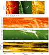 |
Fig. 6. Oscillations captured in larger loop. (a) AIA 171 x − t map of Slit 3 for the time during and after coronal rain. The two vertical blue lines represent the time span from the first appearance of coronal rain until it reaches the footpoint of the loop in the SJI 2796 channel. (b) and (c) Oscillation captured in AIA 304 and SJI 2796, respectively, for the same slit when coronal rain appeared. The x − t maps for AIA channels are produced after motion magnification. All x–t maps are inverted in intensity. |
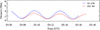 |
Fig. 7. Phase lag of the oscillations detected in different passbands during coronal rain. Curves representing the oscillations observed in slit 3 during rain are shown for both SJI 2796 and AIA 304. The SJI 2796 oscillation amplitude is scaled by a factor of 7 to facilitate a more meaningful comparison. The phase difference between these oscillations is negligible. |
From 03:15 to 03:25 UT, we detect oscillations, O2 in absorption, and O3 in emission in AIA 171 x − t maps (Fig. 4a). These oscillations could be attributed to EUV absorption and CCTR emission originating from rain blobs, as we also observe rain oscillations during this time interval in the SJI 1400 channel with similar amplitude and period (see Fig. 8).
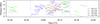 |
Fig. 8. All identified oscillations across various channels on a single timeline with slit distance in the y-axis. The oscillations from different slits are randomly distributed along the slit. The blue dashed lines mark the time interval during which coronal rain is observed in the SJI channels. |
Figure 8 presents a compilation of all detected oscillations in SJI and AIA channels within slits 1 to 7, focusing on the larger loop. The oscillations are arbitrarily shifted along the slit distance for clarity. Within this time line, two blue dashed lines delineate the time frame during which coronal rain is visible in SJI images. Notably, oscillations detected across various slits exhibit an in-phase behavior before, during, and after the occurrence of coronal rain, indicating their standing nature. Furthermore, no evidence of propagating waves is discerned before or after the coronal rain in AIA 171 x − t maps.
We find several oscillations before and after coronal rain to be decayless. However, as discussed in Sect. 3.3.1, we observe a case of amplification during coronal rain. Apart from that, we also observed an oscillation with decreasing period and displacement amplitude during coronal rain in slit 1 of the x − t map of SJI 2796 (Fig. 9). Oscillations of a similar nature were observed by Verwichte & Kohutova (2017) during coronal rain.
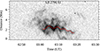 |
Fig. 9. SJI 2796 x − t map of slit 1. The amplitude and period of oscillation captured in the x − t map decay with time. |
The individual cases shown here indicate that the amplitude and period are lower before coronal rain, as seen in AIA 171 x − t maps. The amplitudes and periods are higher during coronal rain, as observed in AIA 304 and SJI channels. During coronal rain, we observe a case of damping and also a case of amplification of oscillations. We also find oscillations of lower amplitude and shorter period after coronal rain in AIA 171.
3.4. Effect of the thermal evolution of the larger loop on the appearance of oscillations
The AIA 171 x − t map in Fig. 6a shows that oscillations are not present between 02:38 and 03:15 UT, while the oscillations are visible between 03:00 and 03:17 UT in AIA 304 and SJI 2796 (Figs. 6b and c). To investigate the impact of the thermal evolution of the loop on the appearance of oscillations in x − t maps, we placed a curved box surrounding the loop top on the bigger loop (left panel of Fig. 10). The average normalized counts in the box are plotted against time for different channels in the right panel. The emission is significant in AIA 304 and SJI 2796 channels when oscillations are visible in the x − t maps for both. The green box shows the time between two maximums in AIA 171 normalized counts. The AIA 171 emission decreases after 02:32 UT, which may be a signature of cooling. The AIA 171 emission is lower between 02:32 and 03:14 UT, which is approximately the same range where oscillations are not present in the AIA 171 x − t map. This suggests that the thermal evolution of the loop can also affect the appearance of oscillations.
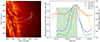 |
Fig. 10. Intensity variation of the loop top in multiple passbands. The left panel shows the cyan box enclosing the loop top at which slit 3 was placed. The right panel shows the temporal evolution of the intensity summed over the cyan box in four passbands. The green box shows the time interval between the maximum of the counts observed in AIA 171. |
3.5. Comparison of average oscillation properties during, before, and after coronal rain
Above, we discuss individual cases of transverse oscillations captured before and after coronal rain in bigger and smaller loops at slit 3 and slit 8. Now, we consider the average properties of decayless oscillations captured in AIA 171 before and after coronal rain. Coronal rain is clearly observable in SJI 1400, 2796, and AIA 304, and oscillations during rain in both absorption and emission are identified in AIA 171. Consequently, we study the average properties of oscillations during coronal rain using these passbands. The left panel of Fig. 11 shows the amplitude of oscillations captured by SJI 1400, 2796, and AIA 304 and 171 during rain. We find that the oscillations captured in these channels have amplitudes ranging from 43 to 415 km with an average of 187 km. Previous studies indicated amplitudes during coronal rain of below 500 km (Antolin & Verwichte 2011) and in the range of 200−400 km (Kohutova & Verwichte 2016). The right panel of Fig. 11 shows the distribution of oscillation amplitudes detected in AIA 171 before and after coronal rain in every slit position at similar locations as observed during rain. The amplitudes have a range of 45−164 km with a mean of 94 km. Similarly low amplitudes have been reported in various active-region loops (Anfinogentov et al. 2015; Mandal et al. 2021; Zhong et al. 2022). Thus, on average, the amplitudes of the oscillations during coronal rain are two times those of the oscillations before and after coronal rain.
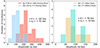 |
Fig. 11. Distribution of oscillation amplitudes captured during (left panel), and before and after coronal rain (right panel). ⟨A⟩ and ⟨σA⟩ denote average amplitude and standard deviation in amplitude, respectively. |
When we look at the distribution of period in Fig. 12, it has a range of 1.4−4.6 min for oscillations detected during rain in SJI 1400, 2796, AIA 304 and 171 passbands, with a mean of 2.9 min, in agreement with earlier reported periods in the range of 1.4−3.3 min in coronal-rain clumps (Antolin & Verwichte 2011). In contrast, the periods range from 1.7 to 2.9 min with a mean of 2.3 min for oscillations captured in the AIA 171 passband before and after rain. Thus, on average, the periods of oscillations during coronal rain are 1.3 times larger than those of oscillations before and after coronal rain. The average amplitude and period before coronal rain as calculated from AIA 171 are 93 ± 28 km and 2.4 ± 0.4 min, respectively, while these values are 94 ± 34 km and 2.2 ± 0.2 min after coronal rain.
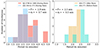 |
Fig. 12. Distribution of oscillation periods captured during (left panel), and before and after coronal rain (right panel). ⟨P⟩ and ⟨σP⟩ denote the average period and standard deviation in the period, respectively. |
We observe coronal rain oscillations in EUV absorption and possible signatures of the oscillations in CCTR emission during coronal rain in AIA 171 x − t maps. The average amplitude of these oscillations is 90 ± 31 km, and the average period is 2.5 ± 0.2 min. The average amplitudes and periods are smaller compared to the same averages calculated from AIA 304 and SJI x − t maps. The oscillations in AIA 171 x − t maps during rain for slit 3 (O2 and O3 in Fig. 6) correspond to a time interval in which rain blobs started descending from the loop top to the footpoint. The oscillation period and amplitude can decrease during this interval, as observed previously in Verwichte & Kohutova (2017). However, the periodic shift in the amplitude and period was not observed in AIA 304 x − t maps, as seen in the SJI 2796 x − t map of slit 1 (Fig. 9). This could be due to the lower resolution of AIA compared to SJI. The underestimation of displacement amplitudes compared to its actual value could be up to 20% after motion magnification (Gao et al. 2022). This could also be a plausible explanation for the lower amplitude in AIA 304 x − t maps during coronal rain found in slit 3. To quantitatively confirm this, we reduced the resolution of SJI 2796 images to match AIA and performed motion magnification. After magnification, we analyzed the oscillation in slit 3 and obtained a period identical to that derived based on AIA 304. However, the amplitude is estimated to be 0.14 ± 0.02 Mm for the SJI 2796 oscillation, while it is 0.16 ± 0.01 Mm for AIA 304, as discussed in Sect. 3.3.2. These amplitudes are quite similar considering their error bars.
3.6. Calculation of loop geometry
We estimated the 3D geometry of the larger loop where slits 1 to 7 are positioned, and it is clearly visible in AIA images. We used the data from EUVI-A/STEREO located at 156.5° Stonyhurst longitude. The lower resolution of EUVI compared to AIA makes it difficult to identify the specific loop in EUVI-A images. However, we exploited the similarity between structures seen in AIA and EUVI-A to distinguish the loop in EUVI-A. Figures 13a and b show the region observed from two viewpoints (e.g. AIA and EUVI-A). We applied the MGN filter in both images to better distinguish between loops. We performed the stereoscopic triangulation using a Python-based GUI tool (Nisticò 2023). The loop fitting was performed using principal component analysis (PCA; Nisticò et al. 2013; Nisticò 2023). The red points in Figs. 13a and b represent the tie-points used for 3D reconstruction.
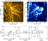 |
Fig. 13. 3D geometry of larger loop and estimation of inclination angle. Panels a and b show the regions of interest as viewed by AIA 171 and EUVI-A 171. The images were processed using the MGN filter. The red points lie on the epipolar line and are used for 3D reconstruction. Panels c–e present the projections of the reconstructed loop in three different planes in the HEEQ coordinate system. The red dashed line indicates the fitted loop. The red and blue arrows show the minor and major axis of the fitted loop, while the green arrow indicates the normal to the loop plane. |
Figures 13c–e presents the projection of the 3D points in blue – calculated after triangulation – in the different orientations of the heliocentric Earth equatorial (HEEQ) coordinates system. The fitted loop is overplotted in red dashed curves. The loop is elliptical in shape with major and minor radii of 0.047 and 0.025 R⊙, respectively. The loop length is estimated to be 140 Mm. The PCA fitting also provides the normal to the loop plane, which can be used to estimate the inclination angle of the loop (Nisticò et al. 2013). The inclination angle of the loop is found to be 36°, which is a crucial parameter for obtaining rain mass. We consider an error of 10% in loop length and 10° in inclination angle.
4. Discussion and conclusions
In this paper, we explore the effect of coronal rain on already present transverse oscillations in coronal loops observed by the AIA and SJI on April 25, 2014. Our analysis of oscillations using SJI suggests oscillation amplitudes of below 1 Mm during coronal rain, motivating us to use the motion magnification technique to capture oscillations in the AIA passbands. We took eight artificial slits in two coronal loops to generate x − t maps for before, during, and after coronal rain. The individual cases presented in this study show the signature of transverse oscillation at the same spatial positions before and after coronal rain in AIA 171. The individual cases show an increase in period and amplitude during coronal rain. The average amplitude during coronal rain is found to be two times higher than before and after coronal rain. The average period is found to be 1.3 times larger during coronal rain.
Verwichte & Kohutova (2017) confirmed the presence of coronal rain oscillations as soon as rain appeared in SJI channels. These authors also pointed out the presence of oscillations in an overlying loop in AIA 171 and 193 passbands. The periods in the overlying loop were similar, but amplitudes were larger than those found during coronal rain in the lower loop. The overlying loop was oscillating about 10 arcsec (7 Mm) above the lower loop. The oscillations were not present after coronal rain in AIA 171 or 193 (see Fig. 7 of Verwichte & Kohutova 2017). However, we see a spatial difference in oscillations of about 1 Mm before, during, and after coronal rain in a few slits, which is only 8 Mm in length. The motion magnification allows us to quantify the oscillations with amplitudes of lower than the resolution of AIA, whereas Verwichte & Kohutova (2017) did not use motion magnification to capture oscillation before and after rain in AIA passbands.
We observe a larger mean period during coronal rain. The loop is denser during coronal rain than prior and is largely evacuated after coronal rain. In the long wavelength limit, kink speed is equal to phase speed and is inversely proportional to the period of oscillation (Nakariakov & Verwichte 2005). The kink speed decreases during coronal rain due to an increase in density, and eventually, the period of oscillation becomes larger. Analytical studies and numerical simulations of transverse oscillations in a cooling coronal loop reveal that the period decreases in a cooling coronal loop with time (Ruderman 2011; Magyar et al. 2015). The plasma cooling changes the density variation along the loop and produces flows from the loop top to the footpoints. Kohutova & Verwichte (2017), using numerical simulations, pointed out that as the condensations reach the loop legs from the loop top, the amplitude and period decrease and are converted into low-amplitude, short-period transverse oscillations. The decrease in the amplitude and period seen after coronal rain could be due to the rearrangement of loop plasma on a small timescale in the whole loop.
We can gain information on density changes due to rain using period variation. For kink oscillations, the square of the period will be proportional to the internal loop density for the constant magnetic field and outside density. Taking a crude assumption that the variation in density is simultaneous at each position of the loop (Verwichte & Kohutova 2017), we can write the following relation,
 (2)
(2)
where ρ and P denote the internal density and period. The subscripts a, b, and d denote the after, before, and during coronal rain scenarios. If we consider the period for oscillations detected in slit 3, which is near the loop top on the larger loop (Fig. 1), then ρd/ρb = 2.25, which means a 125% increase in the internal density in the formation of coronal rain. However, it should be noted that this formula is applicable for density variation occurring in the whole loop, while in coronal rain there is a redistribution of mass and an increase in the density near the loop apex; now, ρa/ρd = 0.38. If we consider a constant volume of the loop, then approximately 60% of the rain mass is drained from the loop due to falling coronal rain.
Assuming that the observed amplitude during coronal rain is solely excited by coronal rain, we can calculate the rain mass fraction present during coronal rain using Eq. (39) of Verwichte et al. (2017). Using oscillation parameters for oscillation detected in slit 3, and loop length and inclination angle obtained after 3D reconstruction, we find the value of rain mass fraction to be 0.41 . We observe that no coronal rain is present in the loop when oscillations are observed before and after coronal rain in AIA 171 (see Fig. 5). This indicates that the oscillations seen in AIA 171 before and after rain are not excited by coronal rain. It is suggested in numerical models and simulations that decayless oscillations can be triggered by footpoint drivers (Nakariakov et al. 2016; Karampelas et al. 2017, 2019; Afanasyev et al. 2020). Considering the footpoint driver being present all the time, the oscillations observed before and after coronal rain might result from footpoint driving. During rain, the observed oscillation properties could be influenced by two drivers: coronal rain and footpoint driving. The amplitude of oscillations can either increase or decrease due to coronal rain depending on whether the two drivers are in phase or out of phase.
The amplitude during the coronal rain is larger than before rain, and given the small observed amplitudes of the oscillations, we can obtain the amplitude specifically associated with rain by subtracting the amplitude resulting from footpoint driving from the overall amplitude during the rain, taking into account the linear regime. In the context of slit 3 on the larger loop, the amplitude attributable to footpoint driving is 0.08 Mm as detected from oscillation O1 in Fig. 6, while the amplitude during rain considering the oscillation from SJI amounts to 0.22 Mm. Consequently, we calculate the amplitude of oscillations solely attributed to rain as 0.14 Mm.
For the second loop (slit 8), the prerain amplitude is 0.09 Mm as obtained from oscillation O1 in Fig. 4. The initial amplitude during rain is 0.11 Mm, which grows by 2.1 times due to rain formation, resulting in the final amplitude being 0.23 Mm. Assuming the amplitude before rain is a consequence of footpoint driving, the amplitude specifically due to rain is found to be 0.14 Mm, which is comparable to the amplitude of previously observed decayless oscillations (Anfinogentov et al. 2015).
We observe signatures of oscillations in AIA 171 during rain, potentially resulting from CCTR emission (Fig. 6). This implies that the amplitude of rain-driven oscillations can indeed be detected using AIA 171 alone, owing to the significant intensity produced by CCTR. If the analysis relies solely on AIA 171, there is a risk of incorrectly using the observed rain-driven oscillations in MHD seismology. The assumption of a coronal density that is lower than the actual value during rain would lead to inaccurate estimation of local conditions in the loop. Assuming a rain density of 1010 cm−3, the calculated magnetic field value from MHD seismology will be  times larger compared to the value obtained using a coronal density of 109 cm−3, with the density ratio considered to be zero.
The results shown in this paper provide evidence of decayless oscillation before and after coronal rain at similar spatial positions. We conclude that increased density due to coronal rain formation can alter the period of already present transverse oscillations in coronal loops. Our study indicates that the contribution to the observed oscillation properties during rain can be attributed to coronal rain and footpoint driving. To check the broad applicability of our results, we need more studies of coronal rain with transverse oscillations and numerical simulations of the same.
Movie
Movie 1 associated with Fig. 1 (Animation1) Access Supplementary Material
Acknowledgments
The authors express their gratitude to the anonymous referee for providing constructive feedback that contributed to the improvement of the paper. A.K.S. is supported by funds of the Council of Scientific & Industrial Research (CSIR), India, under file no. 09/079(2872)/2021-EMR-I. V.P. is supported by SERB start-up research grant (File no. SRG/2022/001687). P.A. acknowledges funding from STFC grants No. ST/R004285/2 and ST/W006790/1. V.P. acknowledges Dr. Erwin Verwichte for useful discussion. A.K.S. and V.P. express gratitude to Tom Van Doorsselaere for insightful discussions. A.K.S. also acknowledges Krishna Prasad S., Ritesh Patel, Bibhuti Kumar Jha, and Satabdwa Majumdar for engaging and helpful discussions. We acknowledge NASA and SDO team for providing AIA data products. SDO is a mission for NASA’s Living With a Star program. IRIS is a NASA small explorer mission developed and operated by LMSAL with mission operations executed at NASA Ames Research Center and major contributions to downlink communications funded by ESA and the Norwegian Space Centre.
References
- Afanasyev, A. N., Van Doorsselaere, T., & Nakariakov, V. M. 2020, A&A, 633, L8 [NASA ADS] [CrossRef] [EDP Sciences] [Google Scholar]
- Anfinogentov, S., & Nakariakov, V. M. 2016, Sol. Phys., 291, 3251 [Google Scholar]
- Anfinogentov, S. A., & Nakariakov, V. M. 2019, ApJ, 884, L40 [CrossRef] [Google Scholar]
- Anfinogentov, S. A., Nakariakov, V. M., & Nisticò, G. 2015, A&A, 583, A136 [NASA ADS] [CrossRef] [EDP Sciences] [Google Scholar]
- Antolin, P. 2020, Plasma Phys. Control. Fusion, 62, 014016 [Google Scholar]
- Antolin, P., & Froment, C. 2022, Front. Astron. Space Sci., 9, 820116 [NASA ADS] [CrossRef] [Google Scholar]
- Antolin, P., & Rouppe van der Voort, L. 2012, ApJ, 745, 152 [Google Scholar]
- Antolin, P., & Verwichte, E. 2011, ApJ, 736, 121 [NASA ADS] [CrossRef] [Google Scholar]
- Antolin, P., Shibata, K., & Vissers, G. 2010, ApJ, 716, 154 [NASA ADS] [CrossRef] [Google Scholar]
- Antolin, P., Vissers, G., & Rouppe van der Voort, L. 2012, Sol. Phys., 280, 457 [NASA ADS] [CrossRef] [Google Scholar]
- Antolin, P., Vissers, G., Pereira, T. M. D., Rouppe van der Voort, L., & Scullion, E. 2015, ApJ, 806, 81 [Google Scholar]
- Antolin, P., Martínez-Sykora, J., & Şahin, S. 2022, ApJ, 926, L29 [NASA ADS] [CrossRef] [Google Scholar]
- Aschwanden, M. J., Fletcher, L., Schrijver, C. J., & Alexander, D. 1999, ApJ, 520, 880 [Google Scholar]
- Auchère, F., Bocchialini, K., Solomon, J., & Tison, E. 2014, A&A, 563, A8 [NASA ADS] [CrossRef] [EDP Sciences] [Google Scholar]
- Auchère, F., Froment, C., Soubrié, E., et al. 2018, ApJ, 853, 176 [Google Scholar]
- Brooks, D. H. 2019, ApJ, 873, 26 [NASA ADS] [CrossRef] [Google Scholar]
- De Groof, A., Berghmans, D., van Driel-Gesztelyi, L., & Poedts, S. 2004, A&A, 415, 1141 [NASA ADS] [CrossRef] [EDP Sciences] [Google Scholar]
- De Groof, A., Bastiaensen, C., Müller, D. A. N., Berghmans, D., & Poedts, S. 2005, A&A, 443, 319 [NASA ADS] [CrossRef] [EDP Sciences] [Google Scholar]
- DelZanna, G., & Mason, H. E. 2003, A&A, 406, 1089 [NASA ADS] [CrossRef] [EDP Sciences] [Google Scholar]
- De Pontieu, B., Title, A. M., Lemen, J. R., et al. 2014, Sol. Phys., 289, 2733 [Google Scholar]
- Doschek, G. A., Mariska, J. T., Warren, H. P., et al. 2007, ApJ, 667, L109 [NASA ADS] [CrossRef] [Google Scholar]
- Duckenfield, T., Anfinogentov, S. A., Pascoe, D. J., & Nakariakov, V. M. 2018, ApJ, 854, L5 [Google Scholar]
- Edwin, P. M., & Roberts, B. 1983, Sol. Phys., 88, 179 [Google Scholar]
- Foullon, C., Verwichte, E., & Nakariakov, V. M. 2004, A&A, 427, L5 [NASA ADS] [CrossRef] [EDP Sciences] [Google Scholar]
- Foullon, C., Verwichte, E., & Nakariakov, V. M. 2009, ApJ, 700, 1658 [NASA ADS] [CrossRef] [Google Scholar]
- Froment, C., Auchère, F., Bocchialini, K., et al. 2015, ApJ, 807, 158 [NASA ADS] [CrossRef] [Google Scholar]
- Froment, C., Auchère, F., Aulanier, G., et al. 2017, ApJ, 835, 272 [Google Scholar]
- Froment, C., Auchère, F., Mikić, Z., et al. 2018, ApJ, 855, 52 [Google Scholar]
- Gao, Y., Tian, H., Van Doorsselaere, T., & Chen, Y. 2022, ApJ, 930, 55 [NASA ADS] [CrossRef] [Google Scholar]
- Hara, H., Watanabe, T., Harra, L. K., et al. 2008, ApJ, 678, L67 [NASA ADS] [CrossRef] [Google Scholar]
- Kaiser, M. L., Kucera, T. A., Davila, J. M., et al. 2008, Space Sci. Rev., 136, 5 [Google Scholar]
- Karampelas, K., Van Doorsselaere, T., & Antolin, P. 2017, A&A, 604, A130 [NASA ADS] [CrossRef] [EDP Sciences] [Google Scholar]
- Karampelas, K., Van Doorsselaere, T., Pascoe, D. J., Guo, M., & Antolin, P. 2019, Front. Astron. Space Sci., 6, 38 [Google Scholar]
- Kawaguchi, I. 1970, PASJ, 22, 405 [NASA ADS] [Google Scholar]
- Kohutova, P., & Verwichte, E. 2016, ApJ, 827, 39 [CrossRef] [Google Scholar]
- Kohutova, P., & Verwichte, E. 2017, A&A, 606, A120 [NASA ADS] [CrossRef] [EDP Sciences] [Google Scholar]
- Lemen, J. R., Title, A. M., Akin, D. J., et al. 2012, Sol. Phys., 275, 17 [Google Scholar]
- Leroy, J.-L. 1972, Sol. Phys., 25, 413 [Google Scholar]
- Magyar, N., Van Doorsselaere, T., & Marcu, A. 2015, A&A, 582, A117 [NASA ADS] [CrossRef] [EDP Sciences] [Google Scholar]
- Mandal, S., Tian, H., & Peter, H. 2021, A&A, 652, L3 [NASA ADS] [CrossRef] [EDP Sciences] [Google Scholar]
- McMath, R. R., & Pettit, E. 1938, ApJ, 88, 244 [NASA ADS] [CrossRef] [Google Scholar]
- Morgan, H., & Druckmüller, M. 2014, Sol. Phys., 289, 2945 [Google Scholar]
- Morgan, H., Habbal, S. R., & Woo, R. 2006, Sol. Phys., 236, 263 [Google Scholar]
- Müller, D. A. N., Peter, H., & Hansteen, V. H. 2004, A&A, 424, 289 [CrossRef] [EDP Sciences] [Google Scholar]
- Nakariakov, V. M., & Verwichte, E. 2005, Liv. Rev. Sol. Phys., 2, 3 [Google Scholar]
- Nakariakov, V. M., Ofman, L., Deluca, E. E., Roberts, B., & Davila, J. M. 1999, Science, 285, 862 [Google Scholar]
- Nakariakov, V. M., Anfinogentov, S. A., Nisticò, G., & Lee, D. H. 2016, A&A, 591, L5 [NASA ADS] [CrossRef] [EDP Sciences] [Google Scholar]
- Nisticò, G. 2023, Sol. Phys., 298, 36 [CrossRef] [Google Scholar]
- Nisticò, G., Verwichte, E., & Nakariakov, V. M. 2013, Entropy, 15, 4520 [CrossRef] [Google Scholar]
- Ofman, L., & Wang, T. J. 2008, A&A, 482, L9 [NASA ADS] [CrossRef] [EDP Sciences] [Google Scholar]
- Okamoto, T. J., Tsuneta, S., Berger, T. E., et al. 2007, Science, 318, 1577 [Google Scholar]
- Oliver, R., Soler, R., Terradas, J., Zaqarashvili, T. V., & Khodachenko, M. L. 2014, ApJ, 784, 21 [Google Scholar]
- Pelouze, G., Auchère, F., Bocchialini, K., et al. 2022, A&A, 658, A71 [NASA ADS] [CrossRef] [EDP Sciences] [Google Scholar]
- Pesnell, W. D., Thompson, B. J., & Chamberlin, P. C. 2012, Sol. Phys., 275, 3 [Google Scholar]
- Reale, F. 2010, Liv. Rev. Sol. Phys., 7, 5 [Google Scholar]
- Roberts, B., Edwin, P. M., & Benz, A. O. 1984, ApJ, 279, 857 [CrossRef] [Google Scholar]
- Ruderman, M. S. 2011, Sol. Phys., 271, 41 [Google Scholar]
- Schrijver, C. J. 2001, Sol. Phys., 198, 325 [Google Scholar]
- Schrijver, C. J., Title, A. M., Berger, T. E., et al. 1999, Sol. Phys., 187, 261 [NASA ADS] [CrossRef] [Google Scholar]
- Shrivastav, A. K., Pant, V., Berghmans, D., et al. 2024, A&A, 685, A36 [NASA ADS] [CrossRef] [EDP Sciences] [Google Scholar]
- Subramanian, S., Tripathi, D., Klimchuk, J. A., & Mason, H. E. 2014, ApJ, 795, 76 [NASA ADS] [CrossRef] [Google Scholar]
- Verwichte, E., & Kohutova, P. 2017, A&A, 601, L2 [NASA ADS] [CrossRef] [EDP Sciences] [Google Scholar]
- Verwichte, E., Antolin, P., Rowlands, G., Kohutova, P., & Neukirch, T. 2017, A&A, 598, A57 [NASA ADS] [CrossRef] [EDP Sciences] [Google Scholar]
- Viall, N. M., & Klimchuk, J. A. 2013, ApJ, 771, 115 [NASA ADS] [CrossRef] [Google Scholar]
- Wang, T., Ofman, L., Davila, J. M., & Su, Y. 2012, ApJ, 751, L27 [Google Scholar]
- Wuelser, J. P., Lemen, J. R., Tarbell, T. D., et al. 2004, in Telescopes and Instrumentation for Solar Astrophysics, eds. S. Fineschi, & M. A. Gummin, SPIE Conf. Ser., 5171, 111 [NASA ADS] [CrossRef] [Google Scholar]
- Zhong, S., Nakariakov, V. M., Kolotkov, D. Y., Verbeeck, C., & Berghmans, D. 2022, MNRAS, 516, 5989 [NASA ADS] [CrossRef] [Google Scholar]
Appendix A: Table
Details of slits and parameters of oscillations.
All Tables
All Figures
|
Fig. 1. Overview of the observation. (a) Full-disk intensity image of the Sun in AIA 171 processed using the MGN technique. The small green box highlights the event location and FOV of SJI. (b) Zoomed-in view of the green box in AIA 171 Å with the loop system. (c)–(e) Approximately simultaneous SJI 1400, 2796, and AIA 304 (radial-gradient-filtered) images. The presence of coronal rain in the loops can be seen. The cyan lines mark the position of artificial slits chosen for generating space-time maps. Slit 8 overlaps the position of a smaller loop. An animation associated with this figure is available online. |
| In the text | |
|
Fig. 2. Example of edge detection in AIA 171 images. The left panel shows the AIA 171 intensity image of the small green box shown in Fig. 1. The fuzziness of the emission is clearly visible. The right panel shows the unsharp masked inverted image of the same FOV in which loop edges are enhanced. |
| In the text | |
|
Fig. 3. Oscillation detection and fitting. (a) Space-time map of Slit 1 near the apex of the loops in SJI 1400 are shown in Fig. 1. The negative intensity is shown in each map. These x − t maps show that the different rain clumps oscillate in phase at varying positions of the slits. The decay-less nature of transverse oscillations is also visible in the x − t maps. (b) The plus symbols mark the centers of the threads over-plotted with the obtained sinusoidal fits, which are represented by red curves. The oscillation properties are derived using sinusoidal fits. |
| In the text | |
|
Fig. 4. Oscillations captured in smaller loop. (a) AIA 171 x − t map of Slit 8 for the time before, during, and after coronal rain. The blue vertical lines indicate the time interval when coronal rain was present in the SJI 2796 passband. The x − t maps for AIA channels are produced after motion magnification. These x − t maps are inverted in intensity. (b) The x − t map of Slit 8 in SJI 2796. The increase in amplitude is clearly visible, and the oscillation is fitted with the red curve. |
| In the text | |
|
Fig. 5. Tracking of the rain blobs along larger loop. Panels a–c depict the location of the curved slit traced along the rain blobs in AIA 304, SJI 2796, and along the loop in AIA 171. Here we aim aim to detect the presence of rain blobs. The placement of the slit is determined based on the trajectory of the rain blobs observed in SJI 2796 images. Panels d–f illustrate the x − t maps associated with the curved slit in AIA 304, SJI 2796, and AIA 171. The black line in the x − t maps represents the estimated position of slit 3 on the curved slit. Around 03:20 UT, the descending rain in EUV absorption is traced by the red dashed line in the AIA 171 x − t map. The line is displayed with an offset to clearly identify the rain features in EUV absorption. The blue dashed line in AIA 304 and SJI 2796 corresponds to the red dashed line in AIA 171. |
| In the text | |
|
Fig. 6. Oscillations captured in larger loop. (a) AIA 171 x − t map of Slit 3 for the time during and after coronal rain. The two vertical blue lines represent the time span from the first appearance of coronal rain until it reaches the footpoint of the loop in the SJI 2796 channel. (b) and (c) Oscillation captured in AIA 304 and SJI 2796, respectively, for the same slit when coronal rain appeared. The x − t maps for AIA channels are produced after motion magnification. All x–t maps are inverted in intensity. |
| In the text | |
|
Fig. 7. Phase lag of the oscillations detected in different passbands during coronal rain. Curves representing the oscillations observed in slit 3 during rain are shown for both SJI 2796 and AIA 304. The SJI 2796 oscillation amplitude is scaled by a factor of 7 to facilitate a more meaningful comparison. The phase difference between these oscillations is negligible. |
| In the text | |
|
Fig. 8. All identified oscillations across various channels on a single timeline with slit distance in the y-axis. The oscillations from different slits are randomly distributed along the slit. The blue dashed lines mark the time interval during which coronal rain is observed in the SJI channels. |
| In the text | |
|
Fig. 9. SJI 2796 x − t map of slit 1. The amplitude and period of oscillation captured in the x − t map decay with time. |
| In the text | |
|
Fig. 10. Intensity variation of the loop top in multiple passbands. The left panel shows the cyan box enclosing the loop top at which slit 3 was placed. The right panel shows the temporal evolution of the intensity summed over the cyan box in four passbands. The green box shows the time interval between the maximum of the counts observed in AIA 171. |
| In the text | |
|
Fig. 11. Distribution of oscillation amplitudes captured during (left panel), and before and after coronal rain (right panel). ⟨A⟩ and ⟨σA⟩ denote average amplitude and standard deviation in amplitude, respectively. |
| In the text | |
|
Fig. 12. Distribution of oscillation periods captured during (left panel), and before and after coronal rain (right panel). ⟨P⟩ and ⟨σP⟩ denote the average period and standard deviation in the period, respectively. |
| In the text | |
|
Fig. 13. 3D geometry of larger loop and estimation of inclination angle. Panels a and b show the regions of interest as viewed by AIA 171 and EUVI-A 171. The images were processed using the MGN filter. The red points lie on the epipolar line and are used for 3D reconstruction. Panels c–e present the projections of the reconstructed loop in three different planes in the HEEQ coordinate system. The red dashed line indicates the fitted loop. The red and blue arrows show the minor and major axis of the fitted loop, while the green arrow indicates the normal to the loop plane. |
| In the text | |
Current usage metrics show cumulative count of Article Views (full-text article views including HTML views, PDF and ePub downloads, according to the available data) and Abstracts Views on Vision4Press platform.
Data correspond to usage on the plateform after 2015. The current usage metrics is available 48-96 hours after online publication and is updated daily on week days.
Initial download of the metrics may take a while.