| Issue |
A&A
Volume 695, March 2025
|
|
|---|---|---|
| Article Number | A2 | |
| Number of page(s) | 21 | |
| Section | Astrophysical processes | |
| DOI | https://doi.org/10.1051/0004-6361/202450989 | |
| Published online | 26 February 2025 | |
Radial X-ray profiles of simulated galaxies
Contributions from hot gas and X-ray binaries
1
Universitäts-Sternwarte, Fakultät für Physik, Ludwig-Maximilians-Universität München, Scheinerstr. 1, 81679 München, Germany
2
INAF, Osservatorio Astronomico di Trieste, Via Tiepolo 11, I-34131 Trieste, Italy
3
IFPU – Institute for Fundamental Physics of the Universe, Via Beirut 2, I-34014 Trieste, Italy
4
Max-Planck-Institut für Astrophysik, Karl-Schwarzschild-Straße 1, 85748 Garching bei München, Germany
⋆ Corresponding author; This email address is being protected from spambots. You need JavaScript enabled to view it.
Received:
4
June
2024
Accepted:
17
January
2025
Abstract
Context. Theoretical models of structure formation predict the presence of a hot gaseous atmosphere around galaxies. While this hot circumgalactic medium (CGM) has been observationally confirmed through UV absorption lines, the detection of its direct X-ray emission remains scarce. Recent results from the eROSITA collaboration have claimed the detection of the CGM out to the virial radius for a stacked sample of Milky Way-mass galaxies.
Aims. We investigate theoretical predictions of the intrinsic CGM X-ray surface brightness (SB) using simulated galaxies and connect them to their global properties, such as the gas temperature, hot gas fraction, and stellar mass.
Methods. We selected a sample of central galaxies from the ultra-high-resolution cosmological volume (48 cMpc h−1) of the Magneticum Pathfinder set of hydrodynamical cosmological simulations. We classified them as star-forming (SF) or quiescent (QU) based on their specific star formation rate (SFR). For each galaxy, we generated X-ray mock data using the X-ray photon simulator PHOX, from which we obtained SB profiles out to the virial radius for different X-ray emitting components; namely, gas, active galactic nuclei (AGNs), and X-ray binaries (XRBs). We fit a β-profile to the gas component of each galaxy and observed trends between its slope and global quantities of the simulated galaxy.
Results. We found marginal differences among the average total SB profile in SF and QU galaxies beyond r > 0.05 Rvir. The relative contribution from hot gas exceeds 70% and is non-zero (≲10%) for XRBs in both galaxy types. At small radii (r < 0.05 Rvir), XRBs dominate the SB profile over the hot gas for QU galaxies. We found positive correlations between the galaxies’ global properties and the normalization of their SB profiles. The fitted β-profile slope is correlated with the total gas luminosity, which, in turn, shows strong connections to the current accretion rate of the central supermassive black hole (SMBH). We found the halo scaling relations to be consistent with the literature.
Key words: methods: numerical / galaxies: star formation / galaxies: statistics / X-rays: binaries / X-rays: galaxies
© The Authors 2025
 Open Access article, published by EDP Sciences, under the terms of the Creative Commons Attribution License (https://creativecommons.org/licenses/by/4.0), which permits unrestricted use, distribution, and reproduction in any medium, provided the original work is properly cited.
This article is published in open access under the Subscribe to Open model. This email address is being protected from spambots. You need JavaScript enabled to view it. to support open access publication.
1. Introduction
In the standard cosmological framework, dark matter (DM) halos attract baryonic matter to form galaxies and clusters of galaxies. The infalling baryonic matter is then shock-heated to X-ray temperatures (T ≳ 106 K), in equilibrium with the gravitational potential well (White & Rees 1978; White & Frenk 1991), forming a gaseous circumgalactic medium (CGM). Due to long cooling times compared to the dynamical time, the CGM is expected to be quasi-static where most cooling processes occur through thermal Bremsstrahlung and line-dominated cooling from different metal species. In addition, there are several feedback mechanisms, such as star formation and feedback from accreting super-massive black holes (SMBHs) powering active galactic nuclei (AGNs), which inject metals and energy into the CGM and cause the CGM to be multi-phase. The interplay between different feedback mechanisms (from, e.g., AGNs) and stellar evolution, as well as the refueling of the inner gas reservoir through cooling processes in the CGM, all play a crucial role in the quenching and growth of galaxies (see review Tumlinson et al. 2017).
The multi-phase structure of the CGM is apparent from observations. Studies of the absorption and emission lines of hydrogen and metals in the UV band revealed the presence of the warm (T ∼ 105 − 6 K) phase of the CGM (Tumlinson et al. 2013; Werk et al. 2016; Burchett et al. 2019) for nearby galaxies which provides further evidence that most of the baryonic matter, including metals, is likely bound to the CGM (Stocke et al. 2013; Werk et al. 2014). Direct X-ray emission from the CGM revealed its hot phase (T ≳ 106 K) in a few nearby massive galaxies (Humphrey et al. 2011; Bogdán et al. 2013, 2015; Buote 2017; Li et al. 2017; Das et al. 2019, 2020) where the signal-to-noise ratio (S/N) allowed them to have reliable detection up to 0.15 R200c1. One of the main challenges in determining the properties of the CGM is the low surface brightness (SB) of hot gas at large galactocentric distances, due to declining gas density. Because the X-ray emissivity of hot plasmas in collisional equilibrium scales with the density squared, the X-ray SB thus declines faster than the density. In addition, the X-ray foreground of the Milky Way (MW) is present in all directions (McCammon et al. 2002) and drowns out most of the signal coming from the low-SB CGM. By performing a stacking analysis of survey galaxies, foreground effects can be somewhat mitigated to obtain a statistical signal from the CGM in the soft X-ray band (SXB), however, this hampers our ability to quantify other global properties of the CGM such as mass, metallicity, and temperature (Anderson et al. 2013, 2015; Li et al. 2018; Comparat et al. 2022; Chadayammuri et al. 2022; Zhang et al. 2024a). Recent results from the extended ROentgen Survey with an Imaging Telescope Array (eROSITA) (Predehl et al. 2021) claim the detection of the CGM out to a radius of 300 kpc, close to the virial radius of MW-mass galaxies (Comparat et al. 2022; Chadayammuri et al. 2022; Zhang et al. 2024a). Both UV and X-ray observations are complemented by analytic models of the temperature and density distribution in the CGM (Faerman et al. 2017, 2020; Faucher-Giguère & Oh 2023).
Most of the emissivity in the SXB is due to specific metals (e.g., oxygen, neon, and iron) which have their transition lines of different ionization states in the energy range of 0.5–2 keV. Recent studies showed that with high-resolution X-ray spectroscopy, it may be possible to directly measure the emissivity of specific metal transitions in certain redshift ranges outside of the MW foreground (Barret et al. 2018; Tashiro et al. 2020; Kraft et al. 2022; Cui et al. 2020). This would enable more detailed studies on metal abundances and temperature of the CGM (Wijers & Schaye 2022; Truong et al. 2023; Bogdán et al. 2023) and give insights into large-scale anisotropies within the hot X-ray atmosphere (Truong et al. 2023; Schellenberger et al. 2024; ZuHone et al. 2024).
A major component of contamination in X-ray emission are unresolved point sources in the form of X-ray binary (XRB) systems in the stellar field of galaxies. Low-mass XRBs (LMXBs), whose cumulative total luminosity scales linearly with the total stellar mass of the galaxy (Gilfanov 2004; Zhang et al. 2012; Lehmer et al. 2016, 2019), are mostly associated with elliptical galaxies with low star formation rates (SFRs, Boroson et al. 2011; Bogdán & Gilfanov 2011; Lehmer et al. 2020). High-mass XRBs (HMXBs) are mostly found in galaxies with high SFR (Grimm et al. 2003; Mineo et al. 2012a). From these earlier studies of HMXBs, it is known that both the total number and total luminosity of HMXBs scale linearly with the SFR of galaxies. More recent studies found evidence for flatter dependence on SFR for galaxies with a low SFR (Kouroumpatzakis et al. 2020; Kyritsis et al. 2025). Deviations from a linear relation can, in principle, be connected to a redshift dependence (Lehmer et al. 2016; Aird et al. 2017), to metallicity (Lehmer et al. 2022), or to stellar age distributions (Lehmer et al. 2017; Gilbertson et al. 2022). However, the observed flatter relation at low SFR is not consistent with low number sampling of HMXB luminosity functions (Gilfanov et al. 2004; Vladutescu-Zopp et al. 2023; Kyritsis et al. 2025). Typically, the total XRB contribution to the total galaxy X-ray luminosity is not exactly known in observations and is modeled empirically for distant galaxies (see e.g., Anderson et al. 2015; Comparat et al. 2022), assuming an absorbed power-law spectrum for unresolved XRB sources. Conservative estimates place the contribution of unresolved XRBs at around < 50% in the SXB (Lehmer et al. 2016; Vladutescu-Zopp et al. 2023). This was recently challenged by Kyritsis et al. (2025), who estimated the contribution from XRB to be ∼80%, which is considerably higher compared to previous studies (Mineo et al. 2012b, 2014; Lehmer et al. 2019; Vladutescu-Zopp et al. 2023; Riccio et al. 2023), using stacking results from the eROSITA all-sky survey 1 (eRASS:1).
This paper aims to shed light on the intrinsic X-ray emission of the CGM in simulated galaxies and connect it to global properties such as halo temperature, gas fraction, and stellar mass. To complement results from stacking procedures, where information about these global properties is partially lost, we investigated simulated galaxies from the Magneticum Pathfinder suite of hydrodynamic cosmological simulations. We made use of the virtual X-ray photon simulator PHOX (Biffi et al. 2012, 2018), which allows for self-consistent and detailed multi-component modeling of the X-ray emission coming from various resolution elements of the simulations. In particular, we have been able to make use of this more accurate modeling to account for signals coming from the broad range of temperatures, metallicities, and densities present in the hot gas of galaxy-sized halos. Additionally, we can directly account for the emission of XRB (Vladutescu-Zopp et al. 2023) and SMBH (Biffi et al. 2018) sources and give accurate estimates of their contribution. The paper is structured as follows. In Sect. 2, we briefly highlight details of the cosmological simulation. In Sect. 3, we briefly describe the PHOX algorithm. In Sect. 4, we present the retrieval of data from the simulation in detail and explain how the X-ray mock data were created. In addition, we give exclusion criteria for a more robust galaxy sample and present our results of X-ray SB profiles on an AGN-cleaned sample in Sect. 5. Finally, we discuss our results in a broader context and summarize our findings in Sect. 6.
2. Cosmological hydrodynamical simulation
In this work, we made use of the Magneticum Pathfinder Simulations2, which comprise a series of state-of-the-art hydrodynamical cosmological simulations. They explore various cosmological volumes at different resolution levels to understand structure formation and the effect of physical processes on all scales. The simulations are performed using an improved version of GADGET 3, which is based on the N-body code GADGET 2 (Springel 2005). Fluid dynamics are solved using a Lagrangian prescription for smoothed particle hydrodynamics (SPH). Improvements in the SPH implementation were made, including a prescription for artificial viscosity and conductivity (Dolag et al. 2005; Beck et al. 2016). The evolution of the baryonic component is described through the subgrid implementation of various physical processes. These comprise radiative gas cooling (Wiersma et al. 2009) and heating from a uniform time-dependent ultraviolet background (Haardt & Madau 2001) and star formation. The latter is treated as a sub-resolution model with a mass-loading rate proportional to SFR and the inclusion of outflows with wind-velocities of vw = 350 km s−1(Springel & Hernquist 2003). The chemical evolution model we implemented is described in Tornatore et al. (2004, 2007). The growth and energy feedback from SMBHs adopts the prescription of Springel (2005) and Di Matteo et al. (2005), along with the modifications described in Fabjan et al. (2010). Numerous studies using the Magneticum simulations have been conducted and demonstrated an appropriate level of consistency with observations. They are able to reproduce the kinematic and morphological properties of galaxies (Teklu et al. 2015, 2017; Remus et al. 2017; Schulze et al. 2018, 2020), as well as chemical properties of galaxies and galaxy clusters (Dolag et al. 2017), and have been employed for studying scaling relations in galaxy clusters (Ragagnin et al. 2019). Furthermore, they present a consistent picture in terms of statistical properties of AGNs (Hirschmann et al. 2014; Steinborn et al. 2016; Biffi et al. 2018) and have thus been studied to investigate environmental signatures of AGN activity and star formation (Rihtaršič et al. 2024). They have also been successfully used in predicting X-ray properties and signatures of galaxies (Vladutescu-Zopp et al. 2023; Bogdán et al. 2023) and galaxy clusters (Ragagnin et al. 2022; ZuHone et al. 2023; Churazov et al. 2023; Bahar et al. 2024).
Similarly to the approach in Vladutescu-Zopp et al. (2023), we used the same ultra-high-resolution run of Magneticum called Box4/uhr. It represents a (48 h−1 cMpc)3 co-moving volume with a mass resolution of mDM = 3.6 × 10⁷ M⊙ and mgas = 7.3 × 10⁶ M⊙ for dark matter and gas respectively corresponding to 5763 particles. The simulation adopts the cosmological parameters from the Wilkinson Microwave Anisotropy Probe (WMAP7) (Komatsu et al. 2011) to model the initial conditions (h = 0.704, ΩM = 0.272, ΩΛ = 0.728, Ωb = 0.0451, and σ8 = 0.809).
3. PHOX X-ray photon simulator
In this section, we describe the general algorithm we used to obtain synthetic X-ray spectra of the baryonic component in the simulations. In particular, we employed the PHOX algorithm (Biffi et al. 2012, 2013) to produce photons according to the intrinsic properties of the simulation. The X-ray photon simulator PHOX operates on three separate modules, as summarized below.
The first module (UNIT 1) is responsible for the conversion of hydrodynamical simulation input into a discrete photon distribution. This is done by considering each possible source in the simulation and computing an idealized spectrum. In the case of a gaseous source, a single temperature APEC thermal emission model (Smith et al. 2001) is assumed (Biffi et al. 2012, 2013), which directly depends on intrinsic properties, such as temperature, density, and total metallicity or variable chemical abundances. In the case of an SMBH source, we would assume an intrinsically absorbed power-law spectrum with variable slope and column density, which mimics torus absorption (Biffi et al. 2018). This allows for all SMBHs to become potential AGNs. In the case of a stellar source, we assume that the underlying stellar population hosts an XRB component. A further distinction between HMXB and LMXB is made based on the stellar age of the host stellar population: HMXB are eligible if the age is less than 30 Myr while LMXB are eligible for ages larger than 1 Gyr following binary evolution calculations (see e.g., Tauris & van den Heuvel 2023). Each seeded XRB also gets assigned an absorbed power-law spectrum with a fixed slope of ΓLMXB = 1.7 for LMXBs and ΓHMXB = 2 for HMXBs, along with a fixed column density of  (Vladutescu-Zopp et al. 2023). Spectral computations make heavy use of the XSPEC3 library interface (Arnaud 1996). Photons are then sampled stochastically from the computed model spectra for each component, assuming a fiducial exposure time and collecting area.
In the second unit (UNIT 2), the photon data generated by the first module are projected along a random direction through the simulation box and stored in photon lists. The projection accounts for redshift effects on photon energies induced by Doppler shifts from the emitting source’s line-of-sight velocity component as well as redshift corrections from angular and luminosity distance. Additionally, we assumed a weak galactic foreground absorption component with column density  cm−2. In all cases, the absorption follows the TBABS model (Wilms et al. 2000), as implemented in XSPEC Additionally, a spatial selection can be considered to only process a small sub-volume of the photon data. As a last step (UNIT 3), the photon lists produced by the second module can be convolved with response matrices of designated X-ray telescopes or can be directly processed by existing X-ray telescope simulators such as SIXTE4 (Dauser et al. 2019).
This approach has been previously applied to study properties of the intercluster medium (ICM) of simulated galaxy clusters (Biffi et al. 2012, 2013, 2014; Biffi & Valdarnini 2015; Cui et al. 2016), the contamination of ICM emission by AGN (Biffi et al. 2018) and to study the contribution of XRB emission in galactic X-ray scaling relations and spectra for simulations of galaxies (Vladutescu-Zopp et al. 2023). The PHOX code is constructed in a general manner such that it can be expanded easily to include the treatment of various X-ray sources which can be constrained from source properties tracked by the simulations.
In Fig. 1, we show the result of running UNIT 1 and UNIT 2 on a face-on disc galaxy from our sample, identified as a “poster child” star-forming disk galaxy in Vladutescu-Zopp et al. (2023). The white outer solid circle corresponds to the virial radius of the galaxy while the inner white dashed circle corresponds to 10% of the virial radius. The color indicates the photon counts per pixel within the energy range of 0.5–2 keV, assuming a fiducial exposure of 1 Ms and effective area 1000 cm2. Black pixels have no photon counts. Each panel shows the same field of view of the galaxy but with a different X-ray emitting component indicated in the top-left corner of the panel.
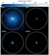 |
Fig. 1. X-ray mock images of the poster-child star-forming disk galaxy from Vladutescu-Zopp et al. (2023). The fiducial orientation of its stellar component is face-on. The outer solid white circle indicates the virial radius. The inner dashed circle indicates 10% of the virial radius. The color indicates the total photon in the SXB per pixel. |
4. Simulated dataset
From the selected cosmological volume described in Sect. 2, we extracted 1319 halos at a redshift of z = 0.0663, which roughly corresponds to an angular diameter distance of 𝒟A ≈ 260 Mpc. They were selected using the SUBFIND algorithm (Springel et al. 2001; Dolag et al. 2009), which defines halos according to a density threshold. For our analysis, we only considered the main central sub-halo within each parent-halo. We further required that the stellar mass of the central is 1010 M⊙ < M∗ < 1012 M⊙ within a sphere of the virial radius, Rvir, around the halo center, while only including particles bound to the central halo according to SUBFIND. The lower mass cut accounts for resolution limitations, the higher mass cut excludes the most massive group-sized halos. Resolution limitations arise for halos in which the number of gas particles is smaller than the number of neighboring particles required for the SPH interpolation (for Mangeticum Box4/uhr: 295 neighbors), which makes hydrodynamical quantities unreliable. Our initial selection is the same as in Vladutescu-Zopp et al. (2023) and consists of 324 star-forming (SF) and 995 quiescent (QU) central galaxies. The classification into SF and QU galaxies is based on the specific star formation rate (sSFR = SFR/M*), where SF galaxies are characterized by logsSFR > −11. For each central galaxy, we derive SFRs from the stellar mass born in the past 100 Myr of the simulation, in line with typical estimators from the literature for X-ray studies of galaxies (Mineo et al. 2012a,b; Lehmer et al. 2016, 2019; Kouroumpatzakis et al. 2020).
Following our initial selection, we obtained X-ray photons by first applying UNIT 1 with a fiducial exposure time of Texp = 2 Ms and effective area Aeff = 1000 cm2 on the full simulation volume. For the gaseous component, the idealized spectrum follows an APEC model scaled to each gas source’s total metallicity. In contrast to Vladutescu-Zopp et al. (2023), we did not impose an intrinsic ISM-absorption component on the gas emission for star-forming central galaxies in addition to the global foreground galactic absorption (see further discussion in Sect. 6). Emission from SMBH and XRB follows the modeling by Biffi et al. (2018) and Vladutescu-Zopp et al. (2023), respectively.
Next, we applied UNIT 2 on each selected halo by projecting the produced photons within a cylindrical volume with a base radius of Rvir and depth of 2 ⋅ Rvir around the halo center. The center is the position of the most-bound particle according to SUBFIND. The chosen line of sight (l.o.s.) is parallel to the z-axis of the underlying simulated volume. We chose Rvir as a scale-free radius to sufficiently represent the gravitationally bound region of each halo. Our analysis does not include an instrumental response because we opted to predict intrinsic properties from the simulations.
From the projected photons we construct surface brightness (SB) profiles by radially binning photons in the plane perpendicular to the l.o.s. centered on the minimum of the gravitational potential. For each radial bin, we take the sum of all photon energies in a chosen energy range and normalize them by the area of the annulus. We thus obtained
 (1)
(1)
for the SB profile, with 𝒟L being the luminosity distance, ϵj and rj the photon energy and its projected radial distance from the center, and Ri the edges of the radial bins, while  assigns the determined SB value to the center of the radial bin. The same construction applies to all considered X-ray components. We note that in this geometric projection, source photons from satellite subhalos in the vicinity of the central are still included. Thus, when constructing the SB profiles of the centrals, the signal may be contaminated by the presence of satellites. To mitigate the influence of satellites on our conclusions, we used the median filter which masks interfering satellites. However, a residual signal remain and thereby affect the results.
Throughout this work, luminosities are given in the rest frame in the energy range of 0.5–2 keV, if not otherwise noted. For the total luminosity, Ltot, of each halo, we integrated the SB profiles up to Rvir and took the sum of each component. By construction, the X-ray emission of each halo was derived from the photons emitted by all the X-ray sources (gas, SMBHs, XRBs) within the halo boundary Rvir. We emphasize that satellites are masked by a median filter, however, their residuals may still affect the results.
4.1. Sample cleaning
After determining the luminosity of each component, we further clean our initial sample by applying exclusion criteria for AGN galaxies which we partially adapt from Lehmer et al. (2016). This allows us to focus our investigation on a well-behaved subsample of galaxies, without dominant contamination from AGN emission. This will provide us with a more solid base to interpret the behavior of SB profiles in normal central galaxies. In particular, we use the following criteria:
-
If the total halo luminosity is
 (2)
(2)in the 0.5-7 keV energy band, we consider the source to be an AGN. This is directly taken from Lehmer et al. (2016) and was also recently employed by Riccio et al. (2023) as an exclusion proxy. We note, however, that the halo luminosity probes much larger radii than in Lehmer et al. (2016).
-
If the integrated luminosity ratio ℓ between SMBH sources (
 ) and the other components (
 and
and  respectively) within the virial radius is
 (3)
(3)then we also consider the source to be an AGN. This second condition was inspired by the requirement to fulfill a pure LX-SFR scaling relation in Lehmer et al. (2016). They allowed the total X-ray luminosity to be three times larger than the SFR scaling relation from Alexander et al. (2005) which is based on the radio luminosity at 1.9 GHz. The argument is that at this frequency, radio emission should mostly come from star formation, while any excess would be associated with an AGN. Without appropriate tracers for radio emission from the simulation, however, we reformulate their criterion to be instead the ratio between the X-ray power from SMBH sources and the combined X-ray power of gas and XRBs. With this we can exclude galaxies which are clearly dominated by an AGN.
-
If
 exceeds the expected luminosity of the central SMBH (L•, see below for definition)
 (4)
(4)we remove the source from our sample. By construction, each SMBH source gets assigned its specific spectral parameters, depending on its bolometric luminosity, such that
 (5)
(5)where
 (see Marconi et al. 2004; Biffi et al. 2018). The second term, σ = 0.1, denotes the maximum of randomized uniform noise which was added to the bolometric correction by Biffi et al. (2018). The latter four terms denote the bolometric correction for the soft X-ray band (0.5–2 keV). The bolometric luminosity (Lbol) of the central SMBH is
  , where Ṁ∙ is the accretion rate of the central SMBH, εr = 0.1 is the radiative efficiency, c is the speed of light. In our modeling, this acts as an upper limit for the luminosity of a single SMBH source, because we employ an effective torus model with intrinsic absorption for SMBH sources which effectively lowers the power output in the soft band. In general, multiple emitting SMBH sources can be present in our simulated galaxies. Thus, the criterion expressed by Eq. (4) is equivalent to excluding systems hosting more than one luminous SMBH source within Rvir, namely, from merging galaxies within the halo.
In Fig. 2, we show  of the projected volume against Ṁ∙ of the central SMBH for the complete sample of galaxies. Colors indicate the ratio ℓ (Eq. (3)). Halos hosting a central AGN galaxy are marked as diamonds. The dashed diagonal line indicates the upper limit that we impose for the collective emission of SMBH sources (see Eq. (4)). From the total sample, 86 SF and 128 QU galaxies are classified as an AGN according to criterion 1. According to criterion 2, 11 SF and 1 QU galaxies have large ℓ and are mostly found for central accretion rates 10−5 M⊙ yr−1 < Ṁ∙ < 10−3 M⊙ yr−1. With criterion 3, we found 31 SF and 21 QU galaxies for which the integrated luminosity,
  , is above the upper limit set by the central SMBH accretion and thus host more than one bright SMBH source within Rvir. Accounting for overlaps, all criteria together thus reduce the full sample to 338 SF and 727 QU normal central galaxies.
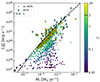 |
Fig. 2. Integrated luminosity of SMBH sources ( |

4.2. Determination of galaxy properties
In this section, we outline the direct estimate of galactic properties from the simulation. In contrast to the X-ray data retrieval, we did not limit ourselves to 2D projected quantities, rather, we made full use of the 3D information available from the simulation. We first selected all resolution elements within a sphere of Rvir around each halo center. Then we filter for all particles which are gravitationally bound to the central subhalo according to the SUBFIND identification. This procedure allows us to remove the substructures for each considered system from our analysis and derive the properties of the central galaxies only. For the stellar mass, M*, we take the sum of the mass of each stellar particle in the matched list. For the hot gas fraction, fgas, and the halo temperature kBT, we first need to select gas particles from the matched list that are considered X-ray emitting. Specifically, we selected the ones that are not star-forming and not multiphase (i.e., those that do not represent cold gas), which have a temperature 105 K ≤ T ≤ 5.85 ⋅ 108 K and an intrinsic density of ρ < 5 ⋅ 10−25 g cm−3. To obtain fgas, we took the ratio between the summed mass of X-ray-emitting gas particles and all gravitationally bound particles (including stars, dark matter, and gas). To derive a single halo temperature, we calculated the emissivity weighted average of the selected gas particles. This approach yields values that are close to a spectral temperature. The emissivity weights were calculated directly from the Astrophysical Plasma Emission Database (APED)5 tables used by APEC (Smith et al. 2001) accounting for individual metal abundances, while assuming the solar abundance from Anders & Grevesse (1989).
5. Galaxy X-ray surface brightness
In this section, we present our findings on the correlation between X-ray surface brightness and the global intrinsic properties of our galaxies. We quantify the contribution of XRBs and SMBH sources to the SB as possible contaminants when determining the properties of the CGM.
Throughout our investigation, we split our full sample into the SF and QU sub-samples. In this way, we were able to probe different mechanisms responsible for maintaining a hot, X-ray-bright gas atmosphere in different galaxy populations. Furthermore, we show SB profiles as a function of a normalized scale-free radius in order to make the sub-sample intrinsically more comparable regardless of differences in physical size. As a reference scale, we chose the virial radius Rvir.
We first investigate the general properties of the QU and SF samples by constructing mean and median profiles of the full subsamples. In Fig. 3a we show the mean (thin lines) and median (thick lines) SB profiles of our complete sample accounting for every source component. The shaded area shows the 16–84 percentile ranges of the median profiles. The median profiles are always lower than the mean profiles because the latter is more sensitive towards extreme outliers as seen from the 84 percentile boundary. Since we include every galaxy irrespective of stellar mass when constructing the mean and median here, we are naturally dominated by the brightest and presumably most massive galaxies. Additionally, the mean enhances the presence of residual structures not associated with an identified satellite which is noticeable by the noisy behavior of the mean at large radii. The median is a more stable estimator here although it is less suited for capturing the SB in the outermost regions, where it is more sensitive to the large number of galaxies with zero emission. The median profile drops to zero SB at ∼0.17 Rvir for the SF sample and at ∼0.22 Rvir for the QU sample. This means that fewer than 50% of the galaxies have a detectable SB beyond those radii, respectively. This is visualized in Fig. 3c, where we show the sample completeness as the fraction of galaxies with non-zero SB at a given radius. When comparing the two sub-samples, the SF sample is centrally brighter than the QU sample both in the median and mean. For radii larger than 0.1 Rvir the mean SB profiles of both samples are comparable with similar normalization and slope, while the median profiles are steeper for SF galaxies. For QU galaxies, the median indicates a slightly more extended SB. According to Fig. 3c this behavior is a result of more galaxies that are bright at larger radii. We note that for large radii, the 16–84 percentiles of the QU and SF samples are identical which indicates that their CGMs have similar properties.
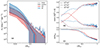 |
Fig. 3. (a): average SB profiles (blue for SF, red for QU) of the normal galaxy sample in the 0.5–2 keV energy band. Thin solid lines indicate the mean total SB. Thick lines indicate the median total SB. The shaded area around the thick lines corresponds to the 16–84 percentile ranges. (b): mean ratio of the SB profiles of one component (gas: dash-dotted; XRB: dashed; SMBH: dotted) towards the total SB. At each radius, we determine the ratio between the SB of one component and the total SB for every galaxy. We take the mean of that ratio by only accounting for galaxies with non-zero SB. (c): sample completeness of the mean ratio in (b). Lines indicate the fraction of galaxies that have non-zero SB at a given radius and thus contribute to the mean ratio in (b). |
To disentangle the contribution of different components to the SB profiles, we computed the ratio between the SB of each component and the total SB for each galaxy. This is shown in Fig. 3b. In each radial bin, we then computed (component-wise) the mean of these ratios only accounting for galaxies with non-zero total SB. In this way, we were able to effectively reduce the number of available galaxies in our sample (cf. Fig. 3c), especially at larger radii; thus, we could consequently inspect details of the SB profile in luminous galaxies. Different line styles in Fig. 3b indicate the mean ratio of gas (dash-dotted), XRB (dashed), and SMBH (dotted) sources towards the total surface brightness of each galaxy, with SF and QU samples in the same colors as in panel a. We note that the mean ratio of each component is not biased by extreme outliers. We verified this by also computing the median ratio of each component, which yielded similar results.
Comparing these trends with the mean and median SB profiles from panel a of Fig. 3, we conclude that the central increase of the SB in SF galaxies is mainly caused by an enhanced contribution from hot gas within ≲0.05Rvir. This is most likely due to the presence of a hot ISM where stellar feedback from active star-forming regions injects energy into the surroundings. Conversely, the XRB component is more dominant for QU galaxies in the central regions. Due to the expected density distributions of stars and hot gas in quenched galaxies, the ISM contribution should be less pronounced in the center compared to XRB. The contribution from SMBH sources is mostly insignificant except for the very center where every galaxy hosts an SMBH. We note that the SMBH considered here would be X-ray faint due to our AGN exclusion. Beyond ∼0.05 Rvir both the SF and QU sample reach similar contribution levels in all components. Interestingly, the average XRB contribution declines from 15–20% at 0.05 Rvir to ≳5% close to Rvir. We attribute this fact to the presence of extended stellar residuals occasionally hosting XRBs.
Given the scatter in each sample, the mean SB profiles of the two classes of galaxies show little qualitative differences. The median SB however hints at SF galaxies being slightly less extended and having steeper profiles compared to QU galaxies. Looking at relative contributions from different sources of the non-zero SB galaxies, we see that most of the difference is coming from the behavior of the ISM gas. In X-ray observations, the distinction between these two classes is also apparent on the ISM level (Bogdán et al. 2013; Kim & Fabbiano 2015; Goulding et al. 2016; Babyk et al. 2018) and is supported by other independent simulation studies using the IllustrisTNG-100 (TNG100) suite (Truong et al. 2020).
5.1. Connection to galaxy properties
In this section, we investigate the shape and slope of median SB profiles of our QU and SF galaxy subsample, while accounting for differences in their global properties. In the self-similar scenario, thermodynamic properties of the hot gaseous atmospheres are directly determined by the depth of the gravitational potential well of the underlying dark matter halo (see e.g., Sarazin 1988). Assuming that the main cooling mechanism is thermal bremsstrahlung, the X-ray luminosity LX of a halo can be expressed as
 (6)
(6)
with
 (7)
(7)
as the gas fraction. We note that the gas fraction is assumed to be constant with mass in the self-similar scenario. In contrast, the true gas fraction of a halo is strongly dependent on stellar and AGN feedback, as well as replenishment and depletion of the gas reservoir. These effects lead to deviations from the self-similar picture which are found in observations of elliptical galaxies as well as of star-forming galaxies (see review by Fabbiano et al. 2019). Based on Eq. (6), we explore the gas fraction fgas and halo temperature kBT (estimated as in Sect. 4.2) of our galaxies and connect them to the SB profiles. We further inspect the relation to their total stellar mass M*.
Measurements of the gas fraction in galaxies have been historically difficult and are typically limited to the innermost regions of the galaxy. For instance, studies using survey data use stacking procedures to enhance the signal of weakly X-ray emitting gas in the outskirts, which makes quantitative statements on gas fractions in individual galaxies impossible. Constraints on the hot gas fraction of individual galaxies are indeed sparse and mostly feasible for massive systems (see e.g., Bogdán et al. 2013; Li et al. 2017; Babyk et al. 2018).
In cosmological simulations, we can estimate directly the galaxies’ intrinsic gas fractions and connect them to X-ray properties. In Fig. 4 we show the gas fraction for each central galaxy in our sample against its stellar mass. Points are colored blue for SF and red for QU galaxies respectively. Additionally, we show histograms of the stellar mass (M*) and the gas fraction (fgas) distributions of our sample which are attached to the respective axis. Dotted lines in the fgas histograms indicate the median value of the respective distribution. The magenta dotted line in the main panel shows the cosmic baryon fraction, fbary, from the simulation. For comparison, we also include measurements of gas fraction and stellar mass from galaxies in the local universe: NGC 720 (Humphrey et al. 2011) and NGC 1521 (Humphrey et al. 2012) (stars); NGC 1961 and NGC 6753 (squares) (Bogdán et al. 2013); star-forming galaxies from (Li et al. 2017); fossil group NGC 6482 (Buote 2017) and compact elliptical galaxy Mrk 1216 (Buote & Barth 2018). We selected these specific observational examples because the gas fractions were obtained from a detailed analysis of mass and density profiles resulting from deep X-ray observations. The mass profiles were then extrapolated to a radius of R200c to calculate the gas fraction. Furthermore, we included gas fraction estimates of the MW (Miller & Bregman 2015; Nicastro et al. 2016) which were obtained from modeling of O VII and O VIII emission and O VII absorption lines in the MW CGM, respectively and also quote the gas fraction at R200. While our sample is consistent with the selected observations in terms of gas fractions, the observational values are biased towards X-ray bright galaxies which may not be representative of the average galaxy population. In the simulated sample, QU galaxies have in general lower gas fractions than SF galaxies and span a larger range of values. We note that the low-value tail of the gas fraction distribution in simulations is dominated by low-mass QU galaxies. Furthermore, the gas fractions reported here do not include satellite galaxies of the central. Therefore, the comparison to observational values might not be fully robust with observations showing higher gas fractions when satellites are included. For comparison, we also report the cosmic fbary value, which is as expected to be larger at all masses.
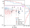 |
Fig. 4. Gas fraction against the stellar mass of central galaxy from our sample with fgas computed according to Eq. (7). SF and QU galaxies are shown in blue and red respectively. Additional symbols with error bars represent values obtained from the literature for comparison. The face color of each symbol indicates SF / QU classification. The magenta line corresponds to the cosmic baryon fraction fbary = 0.167 adopted in the simulation. |
In Fig. 5, we report total SB profiles for the QU (upper panels) and SF (lower panels) samples, for different global intrinsic properties; namely, fgas (left), M* (middle) and kBT (right). Lines with different colors are median profiles binned by the respective property, using the same intervals for both QU and SF galaxies. Given that the property bins do not contain equal numbers of galaxies, constraints would be less strong on the low-number bins. For comparison, we also report the median of the whole SF/QU subsample (dashed black line) from Fig. 3. For a better interpretation of observed profiles and comparisons among different halo sizes, we can define the quantity
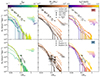 |
Fig. 5. Scale-free median SB profiles of quiescent (top) and star-forming (bottom) galaxies. Galaxies are binned by gas fraction fgas (left), stellar mass M* (center), and emissivity weighted temperature kBT (right). Colors indicate the central value of each bin for the respective quantity. We include SB profiles for NGC 6482 (Buote 2017) and Mrk 1216 (Buote & Barth 2018) in the QU panels and measurements of the extended emission in SF galaxies from Bogdán et al. (2013, 2015), Li et al. (2017) for the SF panels. The violin plots indicate the distribution of ξ (Eq. (8)) within each quantity bin. The horizontal extent of each violin indicates the minimum and maximum value of ξ within the respective bin. The central tick indicates the mean value of ξ. The height of each violin is proportional to the number density of ξ in the bin. The black dashed line is the median profile of the QU and SF sub-sample respectively. |
 (8)
(8)
We chose 300 kpc as a reference scale because it is close to the virial radius of a MW-mass halo and corresponds to the physical galactocentric distance for which CGM emission was detected (Comparat et al. 2022; Chadayammuri et al. 2022; Zhang et al. 2024a). This is used to highlight the distribution of sizes for the halos in each bin, visualized by the violins. In Fig. 5, we also report observed SB profiles for the BCG-like QU galaxies NGC 6482 and Mrk 1216 (Buote 2017; Buote & Barth 2018) and for several local SF galaxies from Bogdán et al. (2013, 2015), Li et al. (2017). We color-coded the observational data points according to the considered property.
5.1.1. Gas fraction
We investigate the impact of the gas fraction on median SB profiles in the first column of Fig. 5. Within the QU sample, median SB profiles have lower normalization and appear less extended with decreasing fgas. Their slope becomes slightly steeper with decreasing fgas. For the lowest fgas bins, the median SB profiles drop to zero before 0.1 Rvir. From the distribution of ξ within each bin (violins), we can infer that QU galaxies residing in more massive halos tend to have higher gas fractions except for the bin with the highest gas fraction (yellow). The highest bin is dominated by small halos with a peak in SB at the center. Compared to NGC 6482 and Mrk 1216, our sample has lower normalization. In fact, NGC 6482 and Mrk 1216 are BCG-like and are expected to be brighter than normal elliptical galaxies (see e.g., Kim & Fabbiano 2015).
For SF median profiles, the normalization in the central regions decreases with decreasing fgas. At the same time, galaxies with lower gas fractions seem to have more extended profiles. This is because the fgas bins are dominated by small halos, which have less extended profiles. Visually, the SF median profiles seem to be steeper compared to the QU sample for the same fgas bins. We caution, however, that the interpretation of trends in the SF sample is more difficult here because of the narrower range in fgas, compared to the QU sample. Since we use the same binning for both subsamples, this leads to fewer non-empty bins in the SF sample with similar size distributions ξ among the bins. A more quantitative approach regarding the steepness of the profiles w.r.t. the gas component will be shown in Sect. 5.3. The median SB profiles of the SF sample are broadly consistent with estimates from observations of massive spiral galaxies (Bogdán et al. 2013; Li et al. 2017). As shown in Fig. 4, reported observations probe similar gas fractions compared to our SF sample but are more massive than the bulk of our SF galaxies. We also note that the annuli for which the SB was extracted in these observations are rather large and thus provide loose constraints. The measured SB for massive spiral galaxies from Bogdán et al. (2013) is higher than our median profiles which is due to the median being dominated by low-mass SF galaxies.
5.1.2. Stellar mass dependence
In the central column of Fig. 5, we show the dependency of median SB profiles on the central galaxy’s stellar mass. The normalization of median profiles in the QU subsample increases with increasing stellar mass. The slope of the profiles remains mostly unaffected by changes in stellar mass and the extent of the profiles decreases with decreasing stellar mass. The distribution in ξ confirms that central galaxies have higher stellar mass in larger halos. The median profiles of all stellar mass bins in the QU case are below the observational sample for the same reason as before. For median SF profiles, the normalization appears to be unaffected by stellar mass. Instead, decreasing stellar mass leads to a steepening of the profiles. The distribution in ξ for each bin shows the same trend as in the QU case. Our median SF profiles are in agreement with observational results in the 0.05 − 0.15 Rvir radial range. For the 0.15 − 0.3 Rvir radial range, our data are consistent with observations. However, the high stellar mass galaxies from Bogdán et al. (2013) are below our median profiles for a similar stellar mass bin while the slightly less massive galaxies from Bogdán et al. (2015) are above the median profiles for similar stellar mass bins in the 0.15 − 0.3 Rvir radial range. This is likely caused by a selection effect of the observational sample compared to our statistical sample. The stellar mass dependency of galaxy X-ray luminosity has been well studied in recent years. Clear correlations have been found for elliptical and spheroidal galaxies with the integrated stellar light (Kim & Fabbiano 2013), for elliptical galaxies with their dynamical mass (Kim & Fabbiano 2015; Forbes et al. 2017). For star-forming galaxies, Aird et al. (2017) showed a connection between the stellar mass and mode of X-ray luminosity. Recent results from the EFEDs field of eROSITA also indicate the presence of a correlation between stellar mass and the SB normalization (Comparat et al. 2022; Chadayammuri et al. 2022; Zhang et al. 2024a).
Generally, a stellar mass trend in the SB should be expected as it can be connected to the gas mass through halo mass relations. The steepening of the profiles in the SF sub-sample indicates a change in the gas density distribution depending on total stellar mass, since the profiles are dominated by gas emission in the outskirts (see Fig. 3). We will quantify this effect and highlight differences between the QU and SF sub-samples in Sect. 5.3.
5.1.3. Temperature
In the right column of Fig. 5, we show the temperature dependence of median SB profiles. With increasing temperature, the median profile of the QU sample in the top panel shows an increase in normalization and becomes more extended. Except for the highest temperature bin, the ξ distribution indicates that larger halos have higher temperatures. The median profile of the highest bin lies in between the other bins in terms of normalization and extent and mostly consists of halos with large ξ, and thus smaller halos. This is not expected from empirical scaling relations, where higher temperatures are associated with more massive galaxies (e.g., Kim & Fabbiano 2015; Goulding et al. 2016; Babyk et al. 2018). Upon inspection, four out of the six halos within the highest temperature bin showed no gas emission and some XRB emission in the central 0.1 Rvir. They have low stellar masses (< 2·1010 M⊙ ) and slightly lower fgas (≂0.06) values. Outside of 0.1 Rvir, they have very shallow gas SB profiles with low normalization and little XRB contribution. Thus, we argue that some recent event removed the central gas of these halos and simultaneously heated their gaseous atmosphere at larger radii. The SF sample shows a weak increase in normalization and radial extent with increasing halo temperature. With decreasing temperature, the profiles again become steeper because the low-temperature bins consist of more small galaxies. The distribution in ξ consistently indicates higher temperatures for larger halos. The SF sample is again in agreement with observations in terms of normalization for all the radial ranges shown. In particular, one galaxy in the sample from Li et al. (2017) has a higher temperature than the highest temperature bin. Again we argue that differences between properties are a result of selection effects in observations.
5.2. SB profiles of the gas component
As shown in Fig. 3, the hot gas is responsible for most of the X-ray emission in our AGN-cleaned sample of galaxies, throughout the majority of the galaxy volume. It is thus interesting to further inspect the gas SB properties separately. This is directly possible in simulations, where we can predict for each galaxy the emission of the contaminating components (i.e., SMBHs and XRBs) individually. In observations, the study of the hot gas distribution of galaxies is more difficult, due to uncertainties regarding contaminants such as the central emission of the SMBH, point sources in the galactic field, background modeling, and instrumental response. Nonetheless, studies of the CGM emission can be attempted through stacking of galaxy spectra, as shown by Oppenheimer et al. (2020), based on mock observations of simulated galaxies extracted from IllustrisTNG and EAGLE simulations. In fact, recent observational studies based on eROSITA data, successfully employed stacking to find emission above the background level from the CGM of MW/M31-like galaxies (Comparat et al. 2022; Chadayammuri et al. 2022; Zhang et al. 2024a).
Here, we confront our findings with these recent eROSITA results, as shown in Fig. 6. In particular, we report the stacking results for the QU_M10.7 and the SF_M10.7 sample from the eFEDs field (Comparat et al. 2022) (Comp22). We use the same mass selection as their M1 mask which removes the signal from bright AGN and is comparable to our AGN cleaned sample. The QU_10.7 sample consists of 7267 quiescent (log(sSFR [yr−1]) < − 11) GAMA matched galaxies in the mass range of M∗ = 1010−11 M⊙ and the SF_M10.7 sample with 9846 star-forming galaxies in the mass range M∗ = 1010.4−11 M⊙. The mass ranges were chosen such that the mean stellar mass in each sample is M∗ = 1010.7 M⊙. The average redshift is 0.2 and 0.23 for QU_M10.7 and SF_M10.7 respectively. In Fig. 6, we also include the best fit β model for the CGM of 30825 eROSITA stacked central galaxies in the MW mass range (M* ∼ 1010.5 − 11) and a median redshift z ∼ 0.08 from Zhang et al. (2024a) (Z24a) (dash-dotted green line). We also include the derived data points together with their error bars as green squares for the aforementioned MW mass range. The contamination of XRBs, AGNs, and satellite galaxies was accounted for through empirical modeling and the fitting was performed on the background-subtracted stacked SB profile. Furthermore, they do not distinguish between star-forming and quiescent galaxies, thus, both are included in their mass range. An improvement w.r.t Comp22 is a more detailed treatment of contamination from satellite galaxies which leads to a steeper profile. We note that their best-fit β-model for the MW mass regime has large errorbars in general but is representative of their full gas profile.
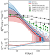 |
Fig. 6. Top: X-ray SB profile of the hot gas component recreating the mass cuts from Comparat et al. (2022). We recreate the observational sample from eFEDs galaxies (Comparat et al. 2022) by replicating their M1 mask for the SF_M10.7 and QU_M10.7 mass bins and show their background-subtracted results. Thin and thick solid-colored lines are the mean and median SB profiles of our sample of galaxies. We apply mass cuts on our sample ranging from M∗ = 1010.46−11 M⊙ for QU galaxies and M∗ = 1010.48−11 M⊙ for SF galaxies and report the total number of galaxies in each stack in the legend. We apply a median filter on the mean stacked profiles (thin solid) to remove substructures. Additionally, we show the best-fit SB profile for the CGM of MW-mass galaxies from Zhang et al. (2024a) which probes a similar stellar mass range. Bottom: ratio of the median stacked profiles (thick, upper panel) of the SF and QU mass-matched sample with the best-fit beta model for MW-mass galaxies from Zhang et al. (2024a). |
For a more faithful comparison, we restrict here to a subsample of our simulated galaxies that more closely resembles the observational selection. By applying exactly the same mass ranges as the QU_M10.7 and SF_M10.7 on our sample, we obtain 93 SF and 645 QU galaxies, which does not reflect the same galaxy number ratio and fails to give the correct mean mass of  . We thus define our mass ranges such that
  , which results in 71 SF (M∗ = 1010.48−11 M⊙) and 247 QU (M∗ = 1010.46−11 M⊙) galaxies. We did not try to recreate an exact match of their stellar mass distribution (see Table 1 in Comp22) because we can not account for the redshift distribution given the fixed redshift of our simulation box. Nonetheless, our chosen mass ranges overlap with the mass ranges and mean redshift presented in Z24a.
In Fig. 6, we plot the mean (thin solid) and median (thick solid) SB profiles of the gas component for our  -matched sub-sample, in blue for SF galaxies and red for QU galaxies. The shaded area corresponds to the 25–75 percentiles and we additionally apply a median filter on the mean profiles only to mask out satellite contribution. Therefore, our treatment of satellites differs from Comp22. They consider a galaxy a satellite if it is within two virial radii of the parent dark matter halo (Comparat et al. 2022) of a more massive nearby galaxy. In contrast, we directly mask the bins affected by satellites and only when showing the mean stacked profile (thin lines) of our samples. The median stacks (thick lines) include satellites but they are affected less. Compared to the profiles by Comp22, we find overall steeper profiles for both the QU and SF samples. However, the procedure in Z24a showed that satellite contamination in Comp22 may still be significant. We directly compare our median stacked results (thick lines) with the best-fit model from Z24a by taking their ratio. For the inner 20 kpc, our QU sample is in good agreement with Z24a while our SF sample has much higher normalization. Beyond this radius, the deviation increases significantly for both the QU and SF samples to more than an order of magnitude due to our median profiles being steeper. Another detail in the observational analysis is the treatment of point sources and nuclear emission in each galaxy. Typically, excess in nuclear emission is attributed to SMBH activity and is consequently removed from the analysis. This could lead to an underestimation of the central SB in observations if the emission is originating from the gas component instead of an AGN.
5.3. Beta profiles of the gaseous component in individual galaxies
The shape of the SB profile associated with the gas component can be further inspected by modeling it with a β profile, as often done in observations. Specifically, we model the SB profiles of the hot gaseous component by fitting both a single β-profile (Sβ) with 3 free parameters or a double β-profile (Dβ) with 6 free parameters. The beta profile takes the form
 (9)
(9)
where S0 is the normalization at r = 0, rc is the core radius (Cavaliere & Fusco-Femiano 1978). The β-profile assumes spherical symmetry of the gas density distribution where the gas is in isothermal equilibrium within the gravitational potential of the galaxy. We use a standard χ2 least-square algorithm in log-space with equal-size radial bins in units of Rvir for each halo to fit the SB radial profile. We assume Poissonian uncertainties on the SB in each radial bin based on the photon counts. We account for satellite galaxies by applying a median filter on the SB profiles which masks affected radial bins. We use the reduced χ2 value to determine the best fit. If the reduced χ2 of single and double β-profile fits are both close to 1, we prefer the single β-profile, which has fewer free parameters. If the best fit is a double β-profile but relative uncertainties in the fitting parameters are large  due to degeneracies, and the single β-model also yields a good fit, we prefer the latter. In cases where neither a single nor a double β-profile adequately describes the data, we label the galaxy as an “undefined” case and do not consider those for the subsequent analysis. In Fig. 7 we show the results of this fitting process. The blue and red colored histograms show the distribution from the SF and QU sample, respectively. Most galaxies in our sample are consistent with a Sβ profile. The most massive halos in our sample are instead better described by the Dβ model. We show exemplary profiles of both categories in Appendix D.1. The undefined cases are galaxies which do not have any surface brightness or have too few (< 10) non-zero radial bins and are exclusively found at low halo masses.
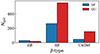 |
Fig. 7. Result of the labeling process after fitting each SB profile with a single and double β profile. The main classification criterion is based on the reduced χ2 as well as parameter degeneracy (see text). |
As a second step, we investigate the relation between the shape of the density profile (quantified via the slope β of the β-profile) and the global properties of the galaxies. To this scope, we restrict our analysis to the subsample of halos that are best modeled by a Sβ profile. In Fig. 8 we show the best-fit single slope β as a function of total gas luminosity LX, gas, stellar mass M*, hot gas fraction fgas and emissivity-weighted hot gas temperature kBT, in panels a, b, c and d respectively. The simulation data points, with error bars, are marked in red and blue to distinguish QU from SF galaxies respectively. The thick colored lines represent the median β of the respective sample for equal-count bins.
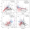 |
Fig. 8. Best-fit slope β of each galaxy’s gas SB profile labeled as a Sβ profile (Eq. (9)) against various halo properties within Rvir: (a) gas luminosity LX, gas; (b) stellar mass M* obtained from stellar resolution elements bound to the parent halo; (c) gas fraction fgas derived from gas resolution elements bound to the parent halo excluding star-forming and low-temperature (< 105 K) gas. In panel (c) the dotted magenta line indicates the cosmic baryon fraction in the simulation; (d) emissivity weighted hot gas temperature Tgas. The exact retrieval of these quantities is outlined in Section 4. The thick solid line in each panel indicates the median value of β. For comparison, we include the sample of massive elliptical galaxies from O’Sullivan et al. (2003) (O’sul+03) and massive star-forming galaxies of Li et al. (2017). Additionally, we compare to β models of the MW from Miller & Bregman (2015) (M&B15) and Nicastro et al. (2016) (model A) in (b) and (c). |
In general, we find that the SB profiles in the SF sample have steeper slopes, compared to the QU sample in all examined properties. Furthermore, uncertainties on the slope increase for larger values of β, due to degeneracy with the core radius, rc. We also note that the overall scatter is large and the two subsamples have significant overlap.
In panel a, we find a strong positive correlation between the slope of the SB profile and LX, gas up to LX, gas ≈ 5 ⋅ 1040 erg s−1 for the QU sample and LX, gas ≈ 1041 erg s−1 for SF galaxies. This indicates that the gas emission becomes more centrally concentrated for more luminous halos in these cases. At higher luminosities, the median slope levels are between β ∼ 0.6 (for QU galaxies) and 0.8 (for SF galaxies). Panel b indicates that our sample spans the largest range in β values at the lowest stellar masses. Despite the large scatter, we still find a moderate tendency for steeper profiles in SF galaxies with lower stellar mass. For stellar mass above 1011 M⊙, β remains around ∼0.6, for both the SF and QU sample. In panel c we find that β is positively correlated with fgas for both QU and SF samples. We also notice that the median slopes of the two sub-samples seem to connect across the full fgas range. This suggests that the distribution of hot gas tends to be more centrally concentrated in galaxies with higher gas fractions. A small fraction of the central increase can be attributed to a hot ISM component in SF galaxies due to SN feedback from newly formed stars. However, in panel d we do not find a clear correlation between steeper slopes and the temperature of the halo. Since the slope is most sensitive to SB outside the core region, this suggests that the steep profiles are an intrinsic property of the halo.
To better interpret the origin of the largest β values, we directly inspected the corresponding profiles. We found that these galaxies either have also large uncertainties on the core radius, rc, or present sharp drops in SB at r ≳ 0.1Rvir. The latter corresponds to a few effective radii for those galaxies. Since we found the steepest slopes in low-mass halos, the compactness of the profiles may be caused by resolution limits in the simulation. In this case, the low density of the halo outskirts is represented by a few resolution elements and it only leads to stochastic effects. At the same time, the smallest values of β are also found in low-mass systems. This is likely a result of strong feedback in the simulation displacing the gas beyond the halo boundary. While the feedback in Magneticum does not directly inject momentum into the gas phase, a strong increase in internal energy can cause the gas to violently redistribute. In the weaker gravitational potential of small halos, this would lead to spreading of the gas to much larger radii. For instance, Angelinelli et al. (2022) showed that for the group and cluster regime of Magneticum, baryon closure is reached at larger radii for lower mass halos at a few R500c if non-gravitational physics is included. Similar effects have been observed in other simulations as well for the galaxy mass regime such as in SIMBA (Sorini et al. 2022), or TNG (Ayromlou et al. 2023) defining the closure radius at the point where the halo gas fraction reaches the cosmic baryon fraction at r ∼ 2 − 3Rvir. Observationally, Z24a also showed that baryon closure is reached at ∼3 Rvir using their stacking results of eRORSITA data.
To cross-validate our statistical results with observations, we compared them with several observational studies. In all panels, we show β for a sample of nearby QU galaxies (gray hexagons), where X-ray properties were obtained from deep Chandra observations including extensive modeling of background sources and contaminants (Babyk et al. 2018). Their studied sample also includes BCG and cG galaxies which we exclude for the comparison. Luminosities and temperatures were directly taken from the aforementioned study. We inferred stellar masses from the central stellar velocity dispersion given for each galaxy in their study using scaling relations from Zahid et al. (2016). Gas fractions were obtained from the given gas masses and the given dynamical mass. We note that X-ray quantities derived in Babyk et al. (2018) were extracted within five effective radii which is smaller than the Rvir in our analysis. While the given profile slopes and halo temperatures should not change significantly at larger radii, properties such as stellar mass and gas fraction are likely lower bounds. In panels a and d, we additionally show a different sample of massive elliptical galaxies (black empty diamonds), by O’Sullivan et al. (2003) who used ROSAT data to obtain SB profiles of massive elliptical galaxies. In panel b we include best-fit slopes for the CGM of MW-mass and M31-mass galaxies from Zhang et al. (2024a) (black filled diamonds) derived from stacking analysis of the first eROSITA full-sky survey (eRASS:1). We also show a sample of massive SF galaxies in all panels from Li et al. (2017) who used data from the X-ray Multi-Mirror Mission (XMM-Newton) for their analysis. In panels b and c there are also values for the Milky Way (MW) derived by Miller & Bregman (2015) and Nicastro et al. (2016). The data by Miller & Bregman (2015) result from a symmetric β-like profile which has been flattened along the axis perpendicular to the galactic disk, and uses XMM-Newton data of O VII and O VIII emission lines from the MW CGM. The values from Nicastro et al. (2016) (model A in their study) refer to a true spherical symmetric profile derived from X-ray absorption lines in Chandra data associated with the MW CGM. We note that our slopes for the SF sample are systematically larger than the slopes from Li et al. (2017) and compared to the MW. Additionally, the gas fractions of the MW and the sample from Li et al. (2017) are lower than those of our SF sample. Interestingly, the slopes from Li et al. (2017) seem to agree better with our QU sample, especially in terms of LX, gas and fgas but are still on the lower side. Our derived slopes are in broad agreement with the β values derived in Babyk et al. (2018), despite being typically higher. While luminosities in their study are similar to ours, they have more high-mass galaxies. Especially in the high stellar mass regime, their SB profiles are shallower. Regarding gas fractions, their sample has a larger range compared to ours. Interestingly, their sample shows a decline in slope with increasing fgas which is in contrast to our results. Furthermore, they probe higher temperatures compared to our analysis which is connected to the higher stellar mass of their galaxies. In general, the temperature of the gaseous halo in observed galaxies is consistent with our sample and also does not show a clear correlation with β. The sample from O’Sullivan et al. (2003) is consistent with slopes derived for our galaxy sample and also contains a few galaxies with β ≳ 1. In their case, larger slopes are likely connected to the environment of their galaxy sample. Most of their targets lie in a cluster or group environment which can in principle affect X-ray properties of the galaxy even after accounting for the cluster emission in spectral modeling.
5.4. Global X-ray luminosity
In Fig. 9, we show total X-ray luminosities of our complete sample (including AGN) as a function of the total mass M500c (gray dots) and compare to scaling relations from Anderson et al. (2015, cyan boxes), Lovisari et al. (2015, red dashed line) and Zhang et al. (2024b, magenta dash-dotted line). We additionally included the six most massive small group-like and cluster-like halos with M∗ > 1012 M⊙ (M500c > 5·1013 M⊙) from the same simulated volume in Fig. 9 which were previously not considered and highlight them as black triangles. For the total luminosity of our sample, we combine the emission of hot gas, XRBs, and SMBHs. Instead of considering the whole Rvir extent for the simulated halos, we extract the properties in the same regions used by Anderson et al. (2015), namely within R500c and [0.15–1] R500c. They obtained their SB measurements from a bootstrapped stacking procedure with data from the Rosat All-Sky Survey (RASS) of SDSS (Sloan Digital Sky Survey) confirmed galaxies in a stellar mass range of 1010−12 M⊙. Luminosities Ltot and LCGM in their study were extracted from stacked SB profiles of central galaxies. These authors derived total masses for their stellar mass bins by forward-modeling of the LX − M500c relation using Ltot from their stacks. With this approach, they did not attempt to derive total masses for halos with M∗ < 1010.8 M⊙ (M500c < 1012.4 M⊙) due to significant contamination from XRBs. We note that Anderson et al. (2015) referred to the radial range [0.15–1] R500c as CGM, which we also adopt here for convenience. The best fit LX − M500c relation from Lovisari et al. (2015) is accounting for selection bias and was derived from a sample of galaxy groups and clusters using XMM-Newton observations. The relation from Zhang et al. (2024b) results from a stacking analysis of central galaxies in eRASS:4 and accounts for source contamination from a central SMBH and XRBs. Thick solid lines in Fig. 9 represent the median of our sample. Colored lines and shaded area represent the contribution of HMXBs (green) and LMXBs (orange) together with their 16–84 percentile which is a direct prediction of our XRB model (see Vladutescu-Zopp et al. 2023 for details). We are thus also able to provide constraints of XRB contribution for the CGM regime. The thin black line is the mean of our sample.
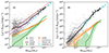 |
Fig. 9. Total X-ray luminosity as a function of halo mass (M500c) (a) within R500c of each galaxy, (b) within (0.15 − 1) R500c. Grey dots represent all galaxies in our full sample, including the AGN systems, with BCG galaxies marked as black triangles. Thin and thick lines represent the mean and median luminosity of our sample, respectively. The contribution from HMXBs and LMXBs in our sample is shown in orange and green together with the 16–84 percentile range as the shaded area. Additionally, we show data from Anderson et al. (2015) (cyan squares) for the total X-ray luminosity within R500 in (a) and CGM luminosity within 0.15 − 1 R500 in (b). The sample consists of central galaxies and results from a stacking analysis using ROSAT data. Their total mass is derived from forward modeling of the LX − M500c relation of gas-dominated halos in their sample. The magenta dash-dotted line is the best fit LX − M500c relation for stacked galaxies in eRASS:4 from Zhang et al. (2024b). The red dashed line shows the bias-corrected best fit LX − M500c relation from Lovisari et al. (2015). |
Generally, the median total luminosity of our sample within R500 (panel a) is in very good agreement with the reported scaling relations from the literature. At intermediate masses, 2 ⋅ 1012 ≲ M500c [M⊙]≲1013, the simulated median relation naturally shows increasing deviations from the relation by Lovisari et al. (2015), whose sample does not include low-mass systems. At lower masses, M500c≲ 2·1012 M⊙, simulation data show a large scatter in luminosity but we still find a broad agreement with the observed relations. The increasing scatter flattens the mean and median at these low halo masses and is driven by extreme outliers, especially at high luminosities. We note that the scaling relations from Zhang et al. (2024b) and Lovisari et al. (2015) have very similar slopes, despite being derived for vastly different halo masses. This hints at a common mechanism shaping the overall matter distribution of all halos.
The median LMXB luminosity follows an almost linear relation with M500c. By construction, LMXB contribution should linearly increase with the stellar mass of the galaxy (Vladutescu-Zopp et al. 2023). Deviations from a linear relation with M500c arise from a non-linear stellar mass function. For the lowest luminosities in our sample, the emission from LMXBs dominates with respect to HMXBs, although the major emitting component remains the hot gas. The median HMXB luminosity increases with halo mass, but its contribution to the total LX is significantly lower compared to LMXBs, except for the highest halo masses.
We note, however, that HMXB contribution is highly dependent on the sample and model assumptions. In A15 for instance, they use an SFR indicator that probes the star formation of the past 300 Myr while we probe star formation in the past 100 Myr. Furthermore, they employed simple scaling relations between SFR and HMXB luminosity while we directly sample the HMXB luminosity functions (see Vladutescu-Zopp et al. 2023). The latter introduces Poissonian noise in the LHMXB scaling relation which steepens the slope of the relation at low SFR (Gilfanov et al. 2004; Vladutescu-Zopp et al. 2023). Moreover, A15 argue that the population of star-forming galaxies increases with lower stellar mass. While this is true in our case as well (see Fig. 4), each stellar mass bin has nonetheless more quiescent galaxies than star-forming galaxies. We also inspected the main sequence for our galaxy sample (shown in Fig. A.1) and found that there are indeed few SF galaxies close to the main sequence at low stellar mass. Hence, we expect SF galaxies below the main sequence to have less contribution from HMXBs, given their SFR, compared to a linear relation.
The mean and median CGM luminosity of our sample (panel b) is in excellent agreement with the stacking results of A15 (cyan) where we used the same values for M500c as in panel a. The contribution of LMXBs and HMXBs to the total CGM luminosity shows steeper trends compared to the total luminosity within R500. This is caused by extended stellar halos associated with the most massive systems which are comprised, for instance, by remnants of disrupted satellites. Moreover, especially LMXBs can contribute significantly towards the CGM luminosity of the least luminous galaxies at low halo masses. In these cases, the hot gas fraction is close to zero and residual LMXB emission must either be associated with a diffuse stellar component outside the central 0.15 R500c. We note that the median and mean CGM luminosity for low-mass halos (M500c < 1012 M⊙) is significantly lower than the total luminosity by at least an order of magnitude. For larger masses, the CGM luminosity becomes comparable to the total luminosity. This implies that most of the emission is centrally concentrated in our sample, which is in line with steeper β-profiles from Sect. 5.3.
6. Discussion
6.1. Inclusion of absorption
By including a weak foreground absorption to model the idealized emission assigned to each gas element, we effectively reduce the X-ray emission in the soft part. Therefore the luminosity retrieved directly from the photon counts, without modeling the spectrum, is in principle a lower limit to the true intrinsic luminosity, even if no instrumental response is included and the ideal photon emission is employed. However, we verified that the foreground absorber does not significantly impact the derived luminosity for each halo, by conducting a simple experiment. We again applied unit 1 of the PHOX algorithm on a sub-volume of the simulation box without the weak foreground absorption component. All other settings were left the same as described in Sect. 4. We compare the total number of photons produced in the case with no absorption and the original setup for the same sub-volume in the energy range 0.5–2 keV. Since we take into account all particles within the simulated sub-volume, we probe a wide range of temperatures and metallicities being affected by absorption. Ultimately, the foreground absorption component, with column density NH = 1020 cm−2, reduces the total number of photons by ≈5% in the considered sub-volume. We thus recompute the luminosities as in Sect. 5 and find that the true intrinsic luminosity is typically underestimated by up to 5% when absorption is included.
Another point worth considering is the inclusion of an intrinsic component mimicking ISM absorption in SF galaxies which we did not include in this study. Typical values for ISM absorption in observed SF galaxies are of the order of ∼1021 cm−2 (see, e.g., Lehmer et al. 2022), which would lead to a reduction of SB in the central 0.1 Rvir in the gas component of SF galaxies by ≳30%, ultimately reducing the normalization of the profiles.
6.2. Beta profiles
We chose a least-squares algorithm in logarithmic space to fit the SB profiles with a single or double β-model. We used the reduced χ2 as the main criterion for comparison, to decide between a Sβ and Dβ model. We manually validated the resulting choice for all halos in the AGN-cleaned sample and confirmed if the fits reached convergence. Additionally, we cross-validated the resulting best-fit parameters using other fitting techniques. On the most massive galaxies within our sample ( ), we employed a likelihood minimization using a C-statistic (Cash 1979), a gradient-descend algorithm as implemented in scipy (Virtanen et al. 2020) and a Markov chain Monte Carlo (MCMC) approach with flat and informed priors using the software package EMCEE (Foreman-Mackey et al. 2013). Both the C-statistic and the gradient-descend method yielded similar best-fit values and agreed with the least-squared method. The MCMC approach was sensitive to the assumed priors and slow to converge. It yielded median fit parameters that were more degenerate than the ones found with the other methods and were systematically lower by ∼10%. Given these results, we decided to rely on the least-square results.
The strong positive correlation between the slope of Sβ halos and their total gas luminosity LX, gas indicates that gas at the center of those halos is emitting more than in the outskirts. This suggests that a feedback mechanism is probably in place, injecting more energy into the central gas. One of the primary sources of energy can be the activity of the SMBH at the center of each galaxy on which we will focus here. In order to quantify the central feedback for each central galaxy in our AGN-cleaned sample, we show LX, gas as a function of the current accretion rate of the central SMBH (Ṁ∙) in Fig. 10. Each data point is colored by the stellar mass of the host galaxy which is the central galaxy of the parent halo. We observe a tight coupling between the total luminosity of the gas component and the current accretion rate of the SMBH. This suggests that the main source of energy in our AGN-cleaned sample appears to be connected to the activity of the central SMBH at all stellar masses. Since we excluded overly X-ray bright AGN from this sample, this correlation is not driven by extreme cases and holds for faint AGNs as well. While the strong link between the SMBH and the regulation of the gas phase is expected (e.g., Hirschmann et al. 2014; Steinborn et al. 2015; Gaspari et al. 2019; Truong et al. 2020, 2021b, 2023), high accretion rates generally also indicate a large gas reservoir in the vicinity of the SMBH. The results in Fig. 10 indicate that the injected energy in the innermost region heats this gas quickly which is immediately reflected in the gas luminosity. An additional mechanism injecting energy into the gas phase is associated with SN feedback. Especially in SF galaxies, SNII feedback can additionally heat the gas and increase its luminosity and may trigger outflows that leave imprints in the CGM SB of SF galaxies (Strickland et al. 2004; Mineo et al. 2012b; Li et al. 2018).
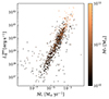 |
Fig. 10. Gas luminosity within Rvir of the AGN cleaned sample as a function of the current accretion rate of the central SMBH Ṁ∙. The colorbar indicates the stellar mass of the galaxy. |
While the β-profile is a simple and well-established model, it is also assuming the gas to be in an isothermal state. Thus it can not account for the expected temperature gradients which are observed for galaxies and galaxy clusters alike (Pratt et al. 2007; Kim et al. 2020). Since the β-profile is a spherically symmetric profile, it can not account for asymmetries in the gas distribution either. In an idealized scenario for disk galaxies, distinct flow patterns are expected to arise with outflows primarily happening perpendicular to the stellar disk and inflows circularizing at the edges of the stellar disk (see e.g., Tumlinson et al. 2017; Stern et al. 2024). Recently, eROSITA revealed large-scale lobes perpendicular to the galactic disk of the MW (Predehl et al. 2020) which are compelling evidence for the aforementioned asymmetries. Simulations showed the presence of such asymmetries in mock X-ray images of simulated galaxies (Truong et al. 2021b, 2023; ZuHone et al. 2024). However, a recent study of edge-on star-forming galaxies in the Virgo galaxy cluster yielded only weak evidence for the presence of extraplanar hot gas (Hou et al. 2024) perpendicular to the stellar disc. We investigated our galaxy sample concerning possible asymmetries by selecting disk-like SF galaxies. We binned them by their inclination angle with respect to the chosen l.o.s. (i.e., the z-axis of the simulation box). We describe the exact setup in Appendix B and show the result in Fig. B.1. We do not find any variation of the SB profiles with inclination angle in our sample. In low-mass galaxies, the resolution limit of the simulation may smooth out emerging asymmetries. Moreover, the feedback from the central SMBH is distributed isotropically in its surroundings which further suppresses asymmetries. A spherically symmetric profile is thus a fair description in our case.
We also verified the validity of the β-model description by reconstructing the X-ray emitting gas mass from the best-fit profiles of the simulated halos represented by a single β model. The deprojected 3D density profile derived from the β-model takes the following form:
 (10)
(10)
where the central gas density is
 (11)
(11)
with μ being the mean molecular weight, mp the proton mass, and
 (12)
(12)
In Eq. (12), n0 denotes the central number density at r = 0, ϵ is the emissivity, B(a, b) represents the validity of the beta function and S0, β, and rc are the same as in Eq. (9) (see also Babyk et al. 2018, for details). The resulting value For each galaxy we computed ϵ assuming an APEC model with the emissivity-weighted average temperature and mass-weighted metallicity of the X-ray emitting gas within Rvir. The resulting total gas mass is then obtained from integrating Eq. (10) up to the virial radius. We show the comparison between the mass of the total X-ray emitting gas in the simulation and the reconstructed gas mass from the beta profile in Fig. 11. We find good correspondence between intrinsic and reconstructed values for high gas masses (Mgas > 1011 M⊙), with some possible bias underestimating the reconstructed gas mass at intermediate mass ranges (1010 ≲ Mgas [M⊙]≲1011). The scatter at very low masses (Mgas < 1010 M⊙) might be driven by a combination of the underlying simplifications as well as large uncertainties on the best-fit rc and β values, originating from a poorly resolved atmosphere.
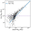 |
Fig. 11. Comparison of the X-ray emitting gas mass from the simulation and the gas mass retrieved from single β-profiles using Eqs. (10)–(12). The solid blue diagonal line indicates equality between the two methods. The horizontal purple dashed line indicates |


Since the plasma in galaxies is generally cooler than in clusters, X-ray emission is mostly dominated by emission lines of various metal species. We therefore investigated possible trends between the slope of Sβ classified halos and their mass-weighted total metallicity. We did not find any correlation between β and the metallicity within 0.1 Rvir or 1 Rvir, which means that a metallicity gradient does not determine the shape of our profiles. Therefore, the β-profile is an adequate description of the gas density in our case.
6.3. Contamination of the CGM emission
One major aspect that must be considered when dealing with the SB of the CGM is contamination from satellites (see also Zhang et al. 2024a). With their stellar mass and potentially high star-formation rates, satellite galaxies can host additional XRB sources. As indicated in Fig. 3b, not only does the gas component contribute towards the extended SB but XRB emission can have non-negligible contribution as well. The show-case galaxy in Fig. 1 illustrates how especially LMXBs can appear as a diffuse component in the halo outskirts. The exact contribution from XRBs is however highly dependent on the assumed spectral model (Lehmer et al. 2016; Vladutescu-Zopp et al. 2023). In our case, we use a relatively high column density when modeling the absorbed power-law spectrum of XRBs compared to other studies (Lehmer et al. 2021; Riccio et al. 2023; Kyritsis et al. 2025). Lower column densities would obviously yield higher contributions from XRBs in the soft band. Figure 1 also shows the presence of actively accreting SMBH point sources which correlate with the position of the subhalos and would be likely masked in observations. Since our AGN-exclusion criteria (Sect. 4.1) ensure that SMBHs associated with satellites are less luminous than the central SMBH, we do not expect significant contamination.
In order to explicitly mask radial bins where satellites are dominant, we used a median filter on the gas SB profiles when fitting β-profiles and when constructing our mean profiles of Fig. 6. While the median filter reliably detected those satellites, the resulting masking of the affected radial bins rendered some of the SB profiles unusable. In those cases, the profile was either dominated by substructures or had too few radial bins left and was consequently undetermined.
Another aspect of XRB contamination comes from the association of XRBs with the main stellar body of a galaxy (see Grimm et al. 2003; Gilfanov 2004). Our detailed model of XRB emission enabled us to quantify XRB contamination not only for the total luminosity (see Fig. 9) but also for the core-excised luminosity. Especially for low-mass halos, XRBs can have a significant contribution to the total luminosity of halos with low SB.
In Fig. 9 we showed that scaling relations between the halo mass M500c and both the total luminosity as well as the core-excised luminosity are in excellent agreement with observations. Especially in the group regime M500c > 1013 M⊙, where the gas component is most dominant, observed scaling relations are perfectly reproduced. Since we include all major emitting components for the total luminosity LX, we also verified that scaling relations are still consistent when only accounting for the gas component. We note that the largest luminosities at low halo masses are associated with galaxies with a bright AGN.
6.4. Scaling with global quantities
Both the QU and SF samples show distinct behavior at different radii with respect to variations in their global properties. In the QU case, all investigated properties mostly affect the normalization of the binned profiles. In the SF case normalization stays the same while the extent of the profiles changes. We know from observations that the hot atmospheres of elliptical galaxies are in hydro-static equilibrium with the gravitational potential and, thus, global properties exhibit a tight relation with the halo mass (Kim & Fabbiano 2015; Forbes et al. 2017; Fabbiano et al. 2019). In SF galaxies, this relation is less clear and observations have shown that the total X-ray luminosity of SF galaxies is only weakly related to halo properties such as temperature (Kim & Fabbiano 2015). Concerning fgas in our SF sample, we would have expected a stronger dependence on the normalization of the SB profiles. From the violin plots in Fig. 5 we can infer that the highest gas fraction bin is comprised preferentially of low mass galaxies for SF galaxies while there are preferentially more massive galaxies in the QU case. This would suggest that a high fraction of the hot gas is located in the halo outskirts of QU galaxies since the whole structure of the SB changes with fgas. This is in line with typical formation scenarios of QU galaxies where energetic feedback events from the central SMBH or major mergers redistributed and heated the gas (see also discussion in Sec. 5.3). In turn, the hot gas appears to be more concentrated towards the center for our SF sample since the normalization of the SB profiles only changes for the inner 0.1 Rvir and is also supported by Fig. 8c. This behavior is however not supported in the literature where shallower profiles are typically observed (Bogdán et al. 2013; Li et al. 2017; Zhang et al. 2024a). The slope also increases for SF galaxies at low masses in our case where the resolution of the simulation may already be too low to properly resolve the hot gas atmosphere outside of 0.1 Rvir.
6.5. Comparison to other simulations
Similar works on the X-ray SB in simulated galaxies have been conducted using different simulation suites. Notably, Oppenheimer et al. (2020) analyzed full eROSTIA mock observations based on EAGLE (Schaye et al. 2015) and IllustrisTNG-100 (TNG100) (Pillepich et al. 2018) simulations. They made use of the pyXSIM package6, which is a python implementation of the PHOX algorithm used in this work (see Sec. 3). When generating the initial photon events from the simulation, they include a model for the MW foreground emission and absorption as well as a model for the background sources. However, they do not directly model the contribution from AGN and X-ray binaries. Additionally, they used SIXTE to account for instrumental effects on the resulting SB profiles. They split their galaxy sample in low (M∗ = 1010.2−10.7 M⊙) and high mass (M∗ = 1010.7−11.2 M⊙) star-forming and quiescent galaxies for both simulation sets and performed a stacking analysis on each respective subsample in a radial range of [10–300] kpc. Their low-mass sample (see their Fig. 2, left) is therefore in a comparable MW mass range w.r.t. our analysis in Fig. 6, on which we will focus here. In general, they find flatter SB profiles for both simulations in the MW mass range compared to our findings, with EAGLE predicting less luminous star-forming galaxies than TNG100. Especially at (r > 100 kpc) we predict an order of magnitude lower SB. At smaller radii, our findings are consistent but interestingly show larger object-by-object variations, which we attribute to the differences in the details of the SMBH feedback treatment in the simulations. Both EAGLE and TNG100 confirm the significant increase in central SB for star-forming galaxies compared to quiescent galaxies which we observe in our simulations. Furthermore, Truong et al. (2020) found that blue galaxies in TNG are an order of magnitude brighter in X-ray than red galaxies at fixed stellar mass, confirming this dichotomy. For radii of r > 50 kpc, we find that SF and QU galaxies have similar SB profiles which is consistent with EAGLE galaxies in Oppenheimer et al. (2020), whereas TNG100 predicts larger SB for star-forming galaxies at all radii. We note that Oppenheimer et al. (2020) considered the X-ray photon emission from the gas included within a sphere of 3 ⋅ R200 around each galaxy, which is significantly larger than the volume inspected here (see Sec. 4). Some contamination in the outskirts, due to gas in the galaxy surrounding not associated with the galaxy itself, can thus be present and contribute to the flattening of the SB profiles. Moreover, those authors performed full mock observations aiming to test CGM detectability, while we focused on intrinsic emission and its connection to the global properties of our galaxies. We thus expect some differences introduced by the instrumental effects, such as in the central SB due to the impact from the eROSITA PSF or in the galaxy outskirts due to the treatment of the background in observations and full mocks.
7. Summary
In this study, we present results on the X-ray SB of simulated galaxies from the Magneticum Pathfinder set of simulations. We made use of the virtual X-ray photon simulator PHOX (Biffi et al. 2012, 2018; Vladutescu-Zopp et al. 2023) to produce highly sophisticated spectral models of individual galaxies, where we properly accounted for the multi-temperature and metallicity distribution of the gaseous component. The emission from SMBH sources and XRBs can be accounted for individually and self-consistently without the need for empirical modeling of their contribution. We accounted for an AGN population in our galaxy sample by applying exclusion criteria motivated by the literature. We focused our analysis on an AGN-cleaned sample uncovering the following aspects:
-
We determined mean and median SB profiles for normal star-forming (log(sSFR) > − 11) and quiescent central galaxies. We then quantified the contribution of different components. We found that our SF sample exhibits an elevated total SB in their central regions, compared to the QU sample up to a scale-free radius of 0.1 Rvir and a comparable SB in the outskirts. The average contribution from XRBs towards the total SB is between 30% and 50% in the inner 0.1 Rvir and ≲10% for larger radii, which we attribute to the presence of a diffuse stellar component in the most massive halos.
-
We compared the median SB profiles of the gas component in a M*-matched subsample of our galaxies to recent observational results from the eROSITA collaboration, where they obtained CGM SB from stacking MW-mass galaxies. A direct comparison with Zhang et al. (2024a) shows a significant deviation for our SF-matched sample, while our QU-matched sample shows reasonable agreement in the center. We found no significant difference between the mean CGM profiles of SF and QU galaxies in our sample for the MW mass range (M* = 1010.5 − 11). Results from Comparat et al. (2022) are in disagreement with our sample, which may be due to instrumental effects and a different treatment of the satellite contribution.
-
We computed hot gas fractions and temperatures for each halo and found positive correlations between the extent and normalization of SB profiles and the respective properties. Correlations are generally stronger for the QU sample than for the SF sample. All our halos have fgas < fbary accounting for hot gas within Rvir. We compared the SB of our sample with SB of observed galaxies for which the same properties (M*, fgas, kBT) were available and found good agreement for SF galaxies. We found a lower normalization for our QU sample, compared to the selected observations. The selected observations are however more consistent with our excluded AGN sample. We attribute this fact to the observational sample including more BCG galaxies, which makes them brighter than typical QU galaxies.
-
We fit β-models to SB profiles of the gas component of our AGN-cleaned sample using a least-square algorithm. We found that most of our sample is best reproduced by a single slope β-profile. We compared the profile slope to intrinsic properties for each halo and found that the SF sample has consistently steeper profiles compared to the QU sample. We found a moderate correlation between steepness and total gas luminosity, which is in agreement with observational results. We found a large scatter in the slope of low M* galaxies in both the QU and SF samples. The slope of the SB profiles seems uncorrelated with fgas and Tgas for SF galaxies and weakly correlated for QU galaxies, while remaining consistent with observational results.
-
We compared the M500c − LX relation of our galaxy sample to stacking results of A15 and Z24b for galaxy-mass halos and also compared to the scaling relations for galaxy groups from Lovisari et al. (2015). While the intrinsic scatter in our sample increases for low halo masses, we still found an excellent agreement with observational results at all halo masses. The scatter is a result of subgrid physics in the underlying cosmological simulation. The estimated median XRB contribution is consistent with theoretical models and can account for the total luminosity of galaxies with the lowest SB.
-
Additionally, we compared the CGM luminosity of our galaxies by using an annulus similar to A15 (r > 0.15 R500c) and found median luminosities in excellent agreement with their stacking results. At low halo masses, LMXBs can contribute significantly to the overall CGM luminosity which may be due to a diffuse stellar component outside of the central galaxy.
-
We find that the main engine for the gas luminosity and consequently the increase in steepness in our sample is the central SMBH of each halo. We find a strong dependence of the global gas luminosity on the current accretion rate of the central SMBH, across the whole range of central galaxy stellar masses investigated. While the SMBH injects feedback energy isotropically into the surroundings in the simulation, the internal energy of neighboring gas is increased. A higher Ṁ∙ generally also suggests that there is more gas in the vicinity of the SMBH to sustain the accretion. The energy is then released close to the SMBH, which leads to a centrally localized increase in luminosity and consequently to a steeper SB profile.
Ultimately, we were able to show that the CGM of galaxies can be resolved in modern cosmological simulations and this offers a unique way of benchmarking observational results. Empirically well-studied relations for the X-ray emission of galaxies arise from the simulation self-consistently and provide predictions for the distribution of the gaseous halo out to the virial radius. However, it is challenging to directly observe the hot CGM in emission due to the emissivity being proportional to the density squared. The detection of the CGM out to large radii has been confirmed in emission using stacking procedures. While stacking can retrieve the average properties of the underlying sample, information about the diversity of trends and scatter in those properties, such as the metallicity, temperature, or gas fraction, is lost. Our study can be therefore useful in improving our understanding of the underlying properties of galaxies and their systematics in commonly adopted observational techniques. In the future, current and proposed X-ray missions using calorimetry-based detectors, such as XRISM (Tashiro et al. 2020) or LEM (Kraft et al. 2022), may provide additional insights by directly measuring gas emission lines and setting more stringent constraints on feedback models and enrichment in the CGM.
In the linear collapse model of structure formation, R200c denotes the radius at which the mean halo density reaches 200 times the critical density of the Universe.
Project web page: www.magneticum.org
v12.12.
Acknowledgments
We thank the anonymous referee for their helpful comments and suggestions which improved the quality of this paper. SVZ and VB acknowledge support by the Deutsche Forschungsgemeinschaft, DFG project nr. 415510302. KD acknowledges support through the COMPLEX project from the European Research Council (ERC) under the European Union’s Horizon 2020 research and innovation program grant agreement ERC-2019-AdG 882679. This research was supported by the Excellence Cluster ORIGINS which is funded by the Deutsche Forschungsgemeinschaft (DFG, German Research Foundation) under Germany’s Excellence Strategy – EXC-2094 – 390783311. The calculations for the hydrodynamical simulations were carried out at the Leibniz Supercomputer Center (LRZ) under the project pr83li. We are especially grateful for the support by M. Petkova through the Computational Center for Particle and Astrophysics (C2PAP). SVZ would like to thank IK and IM for their helpful comments and insightful discussions.
References
- Aird, J., Coil, A. L., & Georgakakis, A. 2017, MNRAS, 465, 3390 [NASA ADS] [CrossRef] [Google Scholar]
- Alexander, D. M., Bauer, F. E., Chapman, S. C., et al. 2005, ApJ, 632, 736 [NASA ADS] [CrossRef] [Google Scholar]
- Anders, E., & Grevesse, N. 1989, Geochim. Cosmochim. Acta, 53, 197 [Google Scholar]
- Anderson, M. E., Bregman, J. N., & Dai, X. 2013, ApJ, 762, 106 [NASA ADS] [CrossRef] [Google Scholar]
- Anderson, M. E., Gaspari, M., White, S. D. M., Wang, W., & Dai, X. 2015, MNRAS, 449, 3806 [NASA ADS] [CrossRef] [Google Scholar]
- Angelinelli, M., Ettori, S., Dolag, K., Vazza, F., & Ragagnin, A. 2022, A&A, 663, L6 [NASA ADS] [CrossRef] [EDP Sciences] [Google Scholar]
- Arnaud, K. A. 1996, in Astronomical Data Analysis Software and Systems V, eds. G. H. Jacoby, & J. Barnes, ASP Conf. Ser., 101, 17 [NASA ADS] [Google Scholar]
- Ayromlou, M., Nelson, D., & Pillepich, A. 2023, MNRAS, 524, 5391 [CrossRef] [Google Scholar]
- Babyk, I. V., McNamara, B. R., Nulsen, P. E. J., et al. 2018, ApJ, 857, 32 [Google Scholar]
- Bahar, Y. E., Bulbul, E., Ghirardini, V., et al. 2024, A&A, 691, A188 [NASA ADS] [CrossRef] [EDP Sciences] [Google Scholar]
- Barret, D., Lam Trong, T., den Herder, J. W., et al. 2018, in Space Telescopes and Instrumentation 2018: Ultraviolet to Gamma Ray, eds. J. W. A. den Herder, S. Nikzad, & K. Nakazawa, SPIE Conf. Ser., 10699, 106991G [NASA ADS] [Google Scholar]
- Beck, A. M., Murante, G., Arth, A., et al. 2016, MNRAS, 455, 2110 [Google Scholar]
- Biffi, V., & Valdarnini, R. 2015, MNRAS, 446, 2802 [NASA ADS] [CrossRef] [Google Scholar]
- Biffi, V., Dolag, K., Böhringer, H., & Lemson, G. 2012, MNRAS, 420, 3545 [NASA ADS] [Google Scholar]
- Biffi, V., Dolag, K., & Böhringer, H. 2013, MNRAS, 428, 1395 [Google Scholar]
- Biffi, V., Sembolini, F., De Petris, M., et al. 2014, MNRAS, 439, 588 [NASA ADS] [CrossRef] [Google Scholar]
- Biffi, V., Dolag, K., & Merloni, A. 2018, MNRAS, 481, 2213 [Google Scholar]
- Bogdán, Á., & Gilfanov, M. 2011, MNRAS, 418, 1901 [Google Scholar]
- Bogdán, Á., Forman, W. R., Vogelsberger, M., et al. 2013, ApJ, 772, 97 [CrossRef] [Google Scholar]
- Bogdán, Á., Vogelsberger, M., Kraft, R. P., et al. 2015, ApJ, 804, 72 [CrossRef] [Google Scholar]
- Bogdán, Á., Khabibullin, I., Kovács, O. E., et al. 2023, ApJ, 953, 42 [CrossRef] [Google Scholar]
- Boroson, B., Kim, D.-W., & Fabbiano, G. 2011, ApJ, 729, 12 [NASA ADS] [CrossRef] [Google Scholar]
- Buote, D. A. 2017, ApJ, 834, 164 [NASA ADS] [CrossRef] [Google Scholar]
- Buote, D. A., & Barth, A. J. 2018, ApJ, 854, 143 [NASA ADS] [CrossRef] [Google Scholar]
- Burchett, J. N., Tripp, T. M., Prochaska, J. X., et al. 2019, ApJ, 877, L20 [NASA ADS] [CrossRef] [Google Scholar]
- Cash, W. 1979, ApJ, 228, 939 [Google Scholar]
- Cavaliere, A., & Fusco-Femiano, R. 1978, A&A, 70, 677 [NASA ADS] [Google Scholar]
- Chadayammuri, U., Bogdán, Á., Oppenheimer, B. D., et al. 2022, ApJ, 936, L15 [NASA ADS] [CrossRef] [Google Scholar]
- Churazov, E., Khabibullin, I. I., Dolag, K., Lyskova, N., & Sunyaev, R. A. 2023, MNRAS, 523, 1209 [NASA ADS] [CrossRef] [Google Scholar]
- Comparat, J., Truong, N., Merloni, A., et al. 2022, A&A, 666, A156 [NASA ADS] [CrossRef] [EDP Sciences] [Google Scholar]
- Cui, W., Power, C., Biffi, V., et al. 2016, MNRAS, 456, 2566 [NASA ADS] [CrossRef] [Google Scholar]
- Cui, W., Chen, L. B., Gao, B., et al. 2020, Journal of Low Temperature Physics, 199, 502 [NASA ADS] [CrossRef] [Google Scholar]
- Das, S., Mathur, S., Gupta, A., et al. 2019, ApJ, 885, 108 [NASA ADS] [CrossRef] [Google Scholar]
- Das, S., Mathur, S., & Gupta, A. 2020, ApJ, 897, 63 [NASA ADS] [CrossRef] [Google Scholar]
- Dauser, T., Falkner, S., Lorenz, M., et al. 2019, A&A, 630, A66 [NASA ADS] [CrossRef] [EDP Sciences] [Google Scholar]
- Di Matteo, T., Springel, V., & Hernquist, L. 2005, Nature, 433, 604 [NASA ADS] [CrossRef] [Google Scholar]
- Dolag, K., Vazza, F., Brunetti, G., & Tormen, G. 2005, MNRAS, 364, 753 [NASA ADS] [CrossRef] [Google Scholar]
- Dolag, K., Borgani, S., Murante, G., & Springel, V. 2009, MNRAS, 399, 497 [Google Scholar]
- Dolag, K., Mevius, E., & Remus, R.-S. 2017, Galaxies, 5, 35 [NASA ADS] [CrossRef] [Google Scholar]
- Fabbiano, G. 2019, in The Chandra X-ray Observatory, eds. B. Wilkes, & W. Tucker, 7 [Google Scholar]
- Fabjan, D., Borgani, S., Tornatore, L., et al. 2010, MNRAS, 401, 1670 [Google Scholar]
- Faerman, Y., Sternberg, A., & McKee, C. F. 2017, ApJ, 835, 52 [NASA ADS] [CrossRef] [Google Scholar]
- Faerman, Y., Sternberg, A., & McKee, C. F. 2020, ApJ, 893, 82 [NASA ADS] [CrossRef] [Google Scholar]
- Faucher-Giguère, C.-A., & Oh, S. P. 2023, ARA&A, 61, 131 [CrossRef] [Google Scholar]
- Forbes, D. A., Alabi, A., Romanowsky, A. J., et al. 2017, MNRAS, 464, L26 [NASA ADS] [CrossRef] [Google Scholar]
- Foreman-Mackey, D., Hogg, D. W., Lang, D., & Goodman, J. 2013, PASP, 125, 306 [Google Scholar]
- Gaspari, M., Eckert, D., Ettori, S., et al. 2019, ApJ, 884, 169 [NASA ADS] [CrossRef] [Google Scholar]
- Gilbertson, W., Lehmer, B. D., Doore, K., et al. 2022, ApJ, 926, 28 [NASA ADS] [CrossRef] [Google Scholar]
- Gilfanov, M. 2004, MNRAS, 349, 146 [NASA ADS] [CrossRef] [Google Scholar]
- Gilfanov, M., Grimm, H. J., & Sunyaev, R. 2004, MNRAS, 351, 1365 [NASA ADS] [CrossRef] [Google Scholar]
- Goulding, A. D., Greene, J. E., Ma, C.-P., et al. 2016, ApJ, 826, 167 [Google Scholar]
- Grimm, H. J., Gilfanov, M., & Sunyaev, R. 2003, MNRAS, 339, 793 [Google Scholar]
- Haardt, F., & Madau, P. 2001, in Clusters of Galaxies and the High Redshift Universe Observed in X-rays, eds. D. M. Tran, & J. T. V. Neumann, 64 [Google Scholar]
- Hirschmann, M., Dolag, K., Saro, A., et al. 2014, MNRAS, 442, 2304 [Google Scholar]
- Hou, M., He, L., Hu, Z., et al. 2024, ApJ, 961, 249 [NASA ADS] [CrossRef] [Google Scholar]
- Humphrey, P. J., Buote, D. A., Canizares, C. R., Fabian, A. C., & Miller, J. M. 2011, ApJ, 729, 53 [CrossRef] [Google Scholar]
- Humphrey, P. J., Buote, D. A., O’Sullivan, E., & Ponman, T. J. 2012, ApJ, 755, 166 [NASA ADS] [CrossRef] [Google Scholar]
- Kim, D.-W., & Fabbiano, G. 2013, ApJ, 776, 116 [NASA ADS] [CrossRef] [Google Scholar]
- Kim, D.-W., & Fabbiano, G. 2015, ApJ, 812, 127 [NASA ADS] [CrossRef] [Google Scholar]
- Kim, D.-W., Traynor, L., Paggi, A., et al. 2020, MNRAS, 492, 2095 [CrossRef] [Google Scholar]
- Komatsu, E., Smith, K. M., Dunkley, J., et al. 2011, ApJS, 192, 18 [Google Scholar]
- Kouroumpatzakis, K., Zezas, A., Sell, P., et al. 2020, MNRAS, 494, 5967 [NASA ADS] [CrossRef] [Google Scholar]
- Kraft, R., Markevitch, M., Kilbourne, C., et al. 2022, ArXiv e-prints [arXiv:2211.09827] [Google Scholar]
- Kyritsis, E., Zezas, A., Haberl, F., et al. 2025, A&A, 694, A128 [NASA ADS] [CrossRef] [EDP Sciences] [Google Scholar]
- Lehmer, B. D., Basu-Zych, A. R., Mineo, S., et al. 2016, ApJ, 825, 7 [Google Scholar]
- Lehmer, B. D., Eufrasio, R. T., Markwardt, L., et al. 2017, ApJ, 851, 11 [NASA ADS] [CrossRef] [Google Scholar]
- Lehmer, B. D., Eufrasio, R. T., Tzanavaris, P., et al. 2019, ApJS, 243, 3 [NASA ADS] [CrossRef] [Google Scholar]
- Lehmer, B. D., Ferrell, A. P., Doore, K., et al. 2020, ApJS, 248, 31 [NASA ADS] [CrossRef] [Google Scholar]
- Lehmer, B. D., Eufrasio, R. T., Basu-Zych, A., et al. 2021, ApJ, 907, 17 [NASA ADS] [CrossRef] [Google Scholar]
- Lehmer, B. D., Eufrasio, R. T., Basu-Zych, A., et al. 2022, ApJ, 930, 135 [NASA ADS] [CrossRef] [Google Scholar]
- Li, J.-T., Bregman, J. N., Wang, Q. D., et al. 2017, ApJS, 233, 20 [NASA ADS] [CrossRef] [Google Scholar]
- Li, J.-T., Bregman, J. N., Wang, Q. D., Crain, R. A., & Anderson, M. E. 2018, ApJ, 855, L24 [NASA ADS] [CrossRef] [Google Scholar]
- Lovisari, L., Reiprich, T. H., & Schellenberger, G. 2015, A&A, 573, A118 [NASA ADS] [CrossRef] [EDP Sciences] [Google Scholar]
- Marconi, A., Risaliti, G., Gilli, R., et al. 2004, MNRAS, 351, 169 [Google Scholar]
- McCammon, D., Almy, R., Apodaca, E., et al. 2002, ApJ, 576, 188 [NASA ADS] [CrossRef] [Google Scholar]
- Miller, M. J., & Bregman, J. N. 2015, ApJ, 800, 14 [NASA ADS] [CrossRef] [Google Scholar]
- Mineo, S., Gilfanov, M., & Sunyaev, R. 2012a, MNRAS, 419, 2095 [Google Scholar]
- Mineo, S., Gilfanov, M., & Sunyaev, R. 2012b, MNRAS, 426, 1870 [NASA ADS] [CrossRef] [Google Scholar]
- Mineo, S., Gilfanov, M., Lehmer, B. D., Morrison, G. E., & Sunyaev, R. 2014, MNRAS, 437, 1698 [NASA ADS] [CrossRef] [Google Scholar]
- Nicastro, F., Senatore, F., Krongold, Y., Mathur, S., & Elvis, M. 2016, ApJ, 828, L12 [NASA ADS] [CrossRef] [Google Scholar]
- Oppenheimer, B. D., Bogdán, Á., Crain, R. A., et al. 2020, ApJ, 893, L24 [NASA ADS] [CrossRef] [Google Scholar]
- O’Sullivan, E., Ponman, T. J., & Collins, R. S. 2003, MNRAS, 340, 1375 [CrossRef] [Google Scholar]
- Pearson, W. J., Wang, L., Hurley, P. D., et al. 2018, A&A, 615, A146 [NASA ADS] [CrossRef] [EDP Sciences] [Google Scholar]
- Pillepich, A., Springel, V., Nelson, D., et al. 2018, MNRAS, 473, 4077 [Google Scholar]
- Pratt, G. W., Böhringer, H., Croston, J. H., et al. 2007, A&A, 461, 71 [NASA ADS] [CrossRef] [EDP Sciences] [Google Scholar]
- Predehl, P., Sunyaev, R. A., Becker, W., et al. 2020, Nature, 588, 227 [CrossRef] [Google Scholar]
- Predehl, P., Andritschke, R., Arefiev, V., et al. 2021, A&A, 647, A1 [EDP Sciences] [Google Scholar]
- Ragagnin, A., Dolag, K., Moscardini, L., Biviano, A., & D’Onofrio, M. 2019, MNRAS, 486, 4001 [Google Scholar]
- Ragagnin, A., Andreon, S., & Puddu, E. 2022, A&A, 666, A22 [NASA ADS] [CrossRef] [EDP Sciences] [Google Scholar]
- Remus, R.-S., Dolag, K., Naab, T., et al. 2017, MNRAS, 464, 3742 [Google Scholar]
- Riccio, G., Yang, G., Małek, K., et al. 2023, A&A, 678, A164 [NASA ADS] [CrossRef] [EDP Sciences] [Google Scholar]
- Rihtaršič, G., Biffi, V., Fabjan, D., & Dolag, K. 2024, A&A, 683, A57 [NASA ADS] [CrossRef] [EDP Sciences] [Google Scholar]
- Sarazin, C. L. 1988, X-ray Emission from Clusters of Galaxies (Cambridge: Cambridge University Press) [Google Scholar]
- Schaye, J., Crain, R. A., Bower, R. G., et al. 2015, MNRAS, 446, 521 [Google Scholar]
- Schellenberger, G., Bogdán, Á., ZuHone, J. A., et al. 2024, ApJ, 969, 85 [Google Scholar]
- Schulze, F., Remus, R.-S., Dolag, K., et al. 2018, MNRAS, 480, 4636 [Google Scholar]
- Schulze, F., Remus, R.-S., Dolag, K., et al. 2020, MNRAS, 493, 3778 [Google Scholar]
- Smith, R. K., Brickhouse, N. S., Liedahl, D. A., & Raymond, J. C. 2001, ApJ, 556, L91 [Google Scholar]
- Sorini, D., Davé, R., Cui, W., & Appleby, S. 2022, MNRAS, 516, 883 [CrossRef] [Google Scholar]
- Springel, V. 2005, MNRAS, 364, 1105 [Google Scholar]
- Springel, V., & Hernquist, L. 2003, MNRAS, 339, 289 [Google Scholar]
- Springel, V., White, S. D. M., Tormen, G., & Kauffmann, G. 2001, MNRAS, 328, 726 [Google Scholar]
- Steinborn, L. K., Dolag, K., Hirschmann, M., Prieto, M. A., & Remus, R.-S. 2015, MNRAS, 448, 1504 [Google Scholar]
- Steinborn, L. K., Dolag, K., Comerford, J. M., et al. 2016, MNRAS, 458, 1013 [Google Scholar]
- Stern, J., Fielding, D., Hafen, Z., et al. 2024, MNRAS, 530, 1711 [NASA ADS] [CrossRef] [Google Scholar]
- Stocke, J. T., Keeney, B. A., Danforth, C. W., et al. 2013, ApJ, 763, 148 [Google Scholar]
- Strickland, D. K., Heckman, T. M., Colbert, E. J. M., Hoopes, C. G., & Weaver, K. A. 2004, ApJS, 151, 193 [Google Scholar]
- Tashiro, M., Maejima, H., Toda, K., et al. 2020, in Space Telescopes and Instrumentation 2020: Ultraviolet to Gamma Ray, eds. J. W. A. den Herder, S. Nikzad, & K. Nakazawa, SPIE Conf. Ser., 11444, 1144422 [NASA ADS] [Google Scholar]
- Tauris, T. M., & van den Heuvel, E. P. J. 2023, Physics of Binary Star Evolution. From Stars to X-ray Binaries and Gravitational Wave Sources (Princeton: Princeton University Press) [Google Scholar]
- Teklu, A. F., Remus, R.-S., Dolag, K., et al. 2015, ApJ, 812, 29 [Google Scholar]
- Teklu, A. F., Remus, R.-S., Dolag, K., & Burkert, A. 2017, MNRAS, 472, 4769 [NASA ADS] [CrossRef] [Google Scholar]
- Tornatore, L., Borgani, S., Matteucci, F., Recchi, S., & Tozzi, P. 2004, MNRAS, 349, L19 [Google Scholar]
- Tornatore, L., Borgani, S., Dolag, K., & Matteucci, F. 2007, MNRAS, 382, 1050 [Google Scholar]
- Truong, N., Pillepich, A., Werner, N., et al. 2020, MNRAS, 494, 549 [NASA ADS] [CrossRef] [Google Scholar]
- Truong, N., Pillepich, A., Nelson, D., Werner, N., & Hernquist, L. 2021a, MNRAS, 508, 1563 [NASA ADS] [CrossRef] [Google Scholar]
- Truong, N., Pillepich, A., & Werner, N. 2021b, MNRAS, 501, 2210 [NASA ADS] [CrossRef] [Google Scholar]
- Truong, N., Pillepich, A., Nelson, D., et al. 2023, MNRAS, 525, 1976 [NASA ADS] [CrossRef] [Google Scholar]
- Tumlinson, J., Thom, C., Werk, J. K., et al. 2013, ApJ, 777, 59 [NASA ADS] [CrossRef] [Google Scholar]
- Tumlinson, J., Peeples, M. S., & Werk, J. K. 2017, ARA&A, 55, 389 [Google Scholar]
- Virtanen, P., Gommers, R., Oliphant, T. E., et al. 2020, Nature Methods, 17, 261 [CrossRef] [Google Scholar]
- Vladutescu-Zopp, S., Biffi, V., & Dolag, K. 2023, A&A, 669, A34 [NASA ADS] [CrossRef] [EDP Sciences] [Google Scholar]
- Werk, J. K., Prochaska, J. X., Tumlinson, J., et al. 2014, ApJ, 792, 8 [NASA ADS] [CrossRef] [Google Scholar]
- Werk, J. K., Prochaska, J. X., Cantalupo, S., et al. 2016, ApJ, 833, 54 [NASA ADS] [CrossRef] [Google Scholar]
- White, S. D. M., & Frenk, C. S. 1991, ApJ, 379, 52 [Google Scholar]
- White, S. D. M., & Rees, M. J. 1978, MNRAS, 183, 341 [Google Scholar]
- Wiersma, R. P. C., Schaye, J., & Smith, B. D. 2009, MNRAS, 393, 99 [NASA ADS] [CrossRef] [Google Scholar]
- Wijers, N. A., & Schaye, J. 2022, MNRAS, 514, 5214 [NASA ADS] [CrossRef] [Google Scholar]
- Wilms, J., Allen, A., & McCray, R. 2000, ApJ, 542, 914 [Google Scholar]
- Zahid, H. J., Geller, M. J., Fabricant, D. G., & Hwang, H. S. 2016, ApJ, 832, 203 [NASA ADS] [CrossRef] [Google Scholar]
- Zhang, Y., Comparat, J., Ponti, G., et al. 2024a, A&A, 690, A267 [NASA ADS] [CrossRef] [EDP Sciences] [Google Scholar]
- Zhang, Y., Comparat, J., Ponti, G., et al. 2024b, A&A, 690, A268 [NASA ADS] [CrossRef] [EDP Sciences] [Google Scholar]
- Zhang, Z., Gilfanov, M., & Bogdán, Á. 2012, A&A, 546, A36 [NASA ADS] [CrossRef] [EDP Sciences] [Google Scholar]
- ZuHone, J., Bahar, Y. E., Biffi, V., et al. 2023, A&A, 675, A150 [NASA ADS] [CrossRef] [EDP Sciences] [Google Scholar]
- ZuHone, J. A., Schellenberger, G., Ogorzałek, A., et al. 2024, ApJ, 967, 49 [NASA ADS] [CrossRef] [Google Scholar]
Appendix A: Galaxy main sequence
In Fig. A.1, we show the SFR–M* relation for our galaxy sample, color-coded by SF (blue) and QU (red) galaxies. The black solid line indicates the observed main sequence from Pearson et al. (2018) in the redshift range 0.2 < z < 0.5. The gray dashed diagonal lines indicate the relation for constant values of sSFR. We note that low-mass SF galaxies lie below the main sequence by 0.5 dex, indicating that they typically have less active star formation than expected.
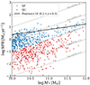 |
Fig. A.1. The main sequence of our total galaxy sample from the simulations. The dashed diagonal lines indicate constant specific star-formation rates in Gyr−1. The solid black line indicates the empirical main sequence from (Pearson et al. 2018) for the redshift range z = 0.2 − 0.5. Blue colors are SF galaxies and red are QU galaxies which we distinguish using the logsSFR [yr−1] = −11 |
Appendix B: Inclination
To quantify the imprints of galaxy orientation with respect to the l.o.s., we investigated the inclination dependence of SB profiles in star-forming disk galaxies. In our framework, the inclination angle i of each galaxy can be computed from the scalar product between the fiducial l.o.s. ( ) and the specific angular momentum of the stellar component (j*), such that
The galaxy would be seen edge-on for cos i = 0 and face-on for cos i = 1. For this test, we only consider star-forming galaxies with a b-value b > −4.35, where
is a measurement of the galaxy morphology (Teklu et al. 2015) and the numerical value was chosen according to Schulze et al. (2020) for disk galaxies. This constrains our sample to only include truly disk-like galaxies, allowing for a meaningful interpretation of the inclination angle. In Fig. B.1 we show mean SB profiles of our disk-like subsample, where galaxies were binned according to the value of cos i (with colors indicating the bin centers). Colored violins have the same meaning as in Fig. 5. We do not find any strong dependence of the SB profile on the galaxy inclination angle. From a theoretical perspective, it is intuitive to assume preferential outflow directions perpendicular to the galactic disc due to the path of least resistance. Numerical studies using different simulations find in fact asymmetric outflow patterns in X-ray mock observations of disc galaxies Truong et al. (2021a, 2023), Schellenberger et al. (2024). Observationally, studies of X-ray emission around disk galaxies did not find however any enhanced signal perpendicular to the disc (Bogdán et al. 2013; Li et al. 2018; Hou et al. 2024).
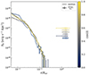 |
Fig. B.1. Similar to Fig. 5. Colors indicate the cosine of the inclination angle of star-forming disk galaxies within each bin. |
Appendix C: Behavior of the AGN sample
In Fig. C.1, we present the mean and median SB profiles of all galaxies excluded by our exclusion criteria from Sec. 4.1. The excluded sample mostly comprises X-ray AGN-dominated galaxies as well as six of the brightest group galaxies (BGGs) with a stellar mass of M∗ > 1012 M⊙. Compared to the cleaned sample, the excluded sample is more than an order of magnitude brighter in the center, which is due to the X-ray bright AGN emission. This can be seen in Fig. C.1(b) where the emission of the central SMBH contributes more than 60% towards the total SB in the center. Furthermore, the difference between SF (blue) and QU (red) galaxies in the central 0.1 Rvir is weaker in the excluded sample than in the cleaned sample. At large radii, profiles are similar to those reported in Fig. 3 for normal galaxies. However, the excluded sample shows slightly more extended emission for SF galaxies. This is caused by the BGGs in the excluded sample which are also highly star-forming. In Fig. C.1 we also include the SB profiles of BCG-like galaxies NGC 6482 (Buote 2017) and Mrk 1216 (Buote & Barth 2018), which are in better agreement with the excluded sample compared to the cleaned sample.
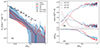 |
Fig. C.1. Same as Fig. 3 for the excluded AGN sample. Additionally, we include SB profiles from BCG like galaxies NGC 6482 and Mrk 1216. |
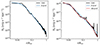 |
Fig. C.2. Exemplary SB profiles (solid black) from the Sβ category (left) and Dβ category (right). The solid blue line shows the best-fit single β-profile and the solid red line shows the best-fit double β-profile. |
Appendix D: Examples
In Fig. D.1, we show two exemplary SB profiles (black) from our sample. The left panel shows a galaxy from the Sβ category which is best represented by a single β-profile (blue). The right panel shows a galaxy from the Dβ category which is best represented by a double β-profile (red). For reference, we also included the best fit single β profile in the right panel to illustrate the difference. We note that the Dβ example also has some substructure within Rvir which is seen as large jumps in the SB profile. Those were masked using a median filter before fitting the profile.
All Figures
|
Fig. 1. X-ray mock images of the poster-child star-forming disk galaxy from Vladutescu-Zopp et al. (2023). The fiducial orientation of its stellar component is face-on. The outer solid white circle indicates the virial radius. The inner dashed circle indicates 10% of the virial radius. The color indicates the total photon in the SXB per pixel. |
| In the text | |
|
Fig. 2. Integrated luminosity of SMBH sources ( |
| In the text | |
|
Fig. 3. (a): average SB profiles (blue for SF, red for QU) of the normal galaxy sample in the 0.5–2 keV energy band. Thin solid lines indicate the mean total SB. Thick lines indicate the median total SB. The shaded area around the thick lines corresponds to the 16–84 percentile ranges. (b): mean ratio of the SB profiles of one component (gas: dash-dotted; XRB: dashed; SMBH: dotted) towards the total SB. At each radius, we determine the ratio between the SB of one component and the total SB for every galaxy. We take the mean of that ratio by only accounting for galaxies with non-zero SB. (c): sample completeness of the mean ratio in (b). Lines indicate the fraction of galaxies that have non-zero SB at a given radius and thus contribute to the mean ratio in (b). |
| In the text | |
|
Fig. 4. Gas fraction against the stellar mass of central galaxy from our sample with fgas computed according to Eq. (7). SF and QU galaxies are shown in blue and red respectively. Additional symbols with error bars represent values obtained from the literature for comparison. The face color of each symbol indicates SF / QU classification. The magenta line corresponds to the cosmic baryon fraction fbary = 0.167 adopted in the simulation. |
| In the text | |
|
Fig. 5. Scale-free median SB profiles of quiescent (top) and star-forming (bottom) galaxies. Galaxies are binned by gas fraction fgas (left), stellar mass M* (center), and emissivity weighted temperature kBT (right). Colors indicate the central value of each bin for the respective quantity. We include SB profiles for NGC 6482 (Buote 2017) and Mrk 1216 (Buote & Barth 2018) in the QU panels and measurements of the extended emission in SF galaxies from Bogdán et al. (2013, 2015), Li et al. (2017) for the SF panels. The violin plots indicate the distribution of ξ (Eq. (8)) within each quantity bin. The horizontal extent of each violin indicates the minimum and maximum value of ξ within the respective bin. The central tick indicates the mean value of ξ. The height of each violin is proportional to the number density of ξ in the bin. The black dashed line is the median profile of the QU and SF sub-sample respectively. |
| In the text | |
|
Fig. 6. Top: X-ray SB profile of the hot gas component recreating the mass cuts from Comparat et al. (2022). We recreate the observational sample from eFEDs galaxies (Comparat et al. 2022) by replicating their M1 mask for the SF_M10.7 and QU_M10.7 mass bins and show their background-subtracted results. Thin and thick solid-colored lines are the mean and median SB profiles of our sample of galaxies. We apply mass cuts on our sample ranging from M∗ = 1010.46−11 M⊙ for QU galaxies and M∗ = 1010.48−11 M⊙ for SF galaxies and report the total number of galaxies in each stack in the legend. We apply a median filter on the mean stacked profiles (thin solid) to remove substructures. Additionally, we show the best-fit SB profile for the CGM of MW-mass galaxies from Zhang et al. (2024a) which probes a similar stellar mass range. Bottom: ratio of the median stacked profiles (thick, upper panel) of the SF and QU mass-matched sample with the best-fit beta model for MW-mass galaxies from Zhang et al. (2024a). |
| In the text | |
|
Fig. 7. Result of the labeling process after fitting each SB profile with a single and double β profile. The main classification criterion is based on the reduced χ2 as well as parameter degeneracy (see text). |
| In the text | |
|
Fig. 8. Best-fit slope β of each galaxy’s gas SB profile labeled as a Sβ profile (Eq. (9)) against various halo properties within Rvir: (a) gas luminosity LX, gas; (b) stellar mass M* obtained from stellar resolution elements bound to the parent halo; (c) gas fraction fgas derived from gas resolution elements bound to the parent halo excluding star-forming and low-temperature (< 105 K) gas. In panel (c) the dotted magenta line indicates the cosmic baryon fraction in the simulation; (d) emissivity weighted hot gas temperature Tgas. The exact retrieval of these quantities is outlined in Section 4. The thick solid line in each panel indicates the median value of β. For comparison, we include the sample of massive elliptical galaxies from O’Sullivan et al. (2003) (O’sul+03) and massive star-forming galaxies of Li et al. (2017). Additionally, we compare to β models of the MW from Miller & Bregman (2015) (M&B15) and Nicastro et al. (2016) (model A) in (b) and (c). |
| In the text | |
|
Fig. 9. Total X-ray luminosity as a function of halo mass (M500c) (a) within R500c of each galaxy, (b) within (0.15 − 1) R500c. Grey dots represent all galaxies in our full sample, including the AGN systems, with BCG galaxies marked as black triangles. Thin and thick lines represent the mean and median luminosity of our sample, respectively. The contribution from HMXBs and LMXBs in our sample is shown in orange and green together with the 16–84 percentile range as the shaded area. Additionally, we show data from Anderson et al. (2015) (cyan squares) for the total X-ray luminosity within R500 in (a) and CGM luminosity within 0.15 − 1 R500 in (b). The sample consists of central galaxies and results from a stacking analysis using ROSAT data. Their total mass is derived from forward modeling of the LX − M500c relation of gas-dominated halos in their sample. The magenta dash-dotted line is the best fit LX − M500c relation for stacked galaxies in eRASS:4 from Zhang et al. (2024b). The red dashed line shows the bias-corrected best fit LX − M500c relation from Lovisari et al. (2015). |
| In the text | |
|
Fig. 10. Gas luminosity within Rvir of the AGN cleaned sample as a function of the current accretion rate of the central SMBH Ṁ∙. The colorbar indicates the stellar mass of the galaxy. |
| In the text | |
|
Fig. 11. Comparison of the X-ray emitting gas mass from the simulation and the gas mass retrieved from single β-profiles using Eqs. (10)–(12). The solid blue diagonal line indicates equality between the two methods. The horizontal purple dashed line indicates |
| In the text | |
|
Fig. A.1. The main sequence of our total galaxy sample from the simulations. The dashed diagonal lines indicate constant specific star-formation rates in Gyr−1. The solid black line indicates the empirical main sequence from (Pearson et al. 2018) for the redshift range z = 0.2 − 0.5. Blue colors are SF galaxies and red are QU galaxies which we distinguish using the logsSFR [yr−1] = −11 |
| In the text | |
|
Fig. B.1. Similar to Fig. 5. Colors indicate the cosine of the inclination angle of star-forming disk galaxies within each bin. |
| In the text | |
|
Fig. C.1. Same as Fig. 3 for the excluded AGN sample. Additionally, we include SB profiles from BCG like galaxies NGC 6482 and Mrk 1216. |
| In the text | |
|
Fig. C.2. Exemplary SB profiles (solid black) from the Sβ category (left) and Dβ category (right). The solid blue line shows the best-fit single β-profile and the solid red line shows the best-fit double β-profile. |
| In the text | |
Current usage metrics show cumulative count of Article Views (full-text article views including HTML views, PDF and ePub downloads, according to the available data) and Abstracts Views on Vision4Press platform.
Data correspond to usage on the plateform after 2015. The current usage metrics is available 48-96 hours after online publication and is updated daily on week days.
Initial download of the metrics may take a while.