| Issue |
A&A
Volume 694, February 2025
|
|
|---|---|---|
| Article Number | A276 | |
| Number of page(s) | 16 | |
| Section | Extragalactic astronomy | |
| DOI | https://doi.org/10.1051/0004-6361/202452915 | |
| Published online | 19 February 2025 | |
Looking into the faintEst WIth MUSE (LEWIS): Exploring the nature of ultra-diffuse galaxies in the Hydra-I cluster
II. Stellar kinematics and dynamical masses
1
INAF – Astronomical Observatory of Capodimonte, Salita Moiariello 16, I-80131 Naples, Italy
2
University of Naples “Federico II”, C.U. Monte Sant’Angelo, Via Cinthia, 80126 Naples, Italy
3
Finnish Centre for Astronomy with ESO (FINCA), FI-20014 University of Turku, Finland
4
Tuorla Observatory, Department of Physics and Astronomy, FI-20014 University of Turku, Finland
5
European Southern Observatory, Karl-Schwarzschild-Strasse 2, 85748 Garching bei München, Germany
6
Centre for Astrophysics & Supercomputing, Swinburne University of Technology, Hawthorn, VIC 3122, Australia
7
INAF – Osservatorio Astronomico di Padova, Vicolo dell’Osservatorio 5, I-35122 Padova, Italy
8
Dipartimento di Fisica e Astronomia “G. Galilei”, Università di Padova, vicolo dell’Osservatorio 3, I-35122 Padova, Italy
9
INAF – Astronomical Observatory of Abruzzo, Via Maggini, 64100 Teramo, Italy
10
Institute of Astronomy, University of Cambridge, Madingley Road, Cambridge CB3 0HA, UK
11
Instituto de Astrofísica de Canarias, Calle Vía Laáctea s/n, E-38205 La Laguna, Tenerife, Spain
12
Departamento de Astrofísica, Universidad de La Laguna, Av. del Astrofísico Francisco Sánchez s/n, E-38206 La Laguna, Tenerife, Spain
13
SRON Netherlands Institute for Space Research, Landleven 12, 9747 AD Groningen, The Netherlands
14
Kapteyn Astronomical Institute, University of Groningen, Postbus 800 9700 AV Groningen, The Netherlands
15
European Southern Observatory, Alonso de Cordova 3107, Vitacura, Santiago, Chile
16
Gran Sasso Science Institute, viale Francesco Crispi 7, I-67100 L’Aquila, Italy
17
Sub-Dep. of Astrophysics, Dep. of Physics, University of Oxford, Denys Wilkinson Building, Keble Road, Oxford OX1 3RH, United Kingdom
18
Armagh Observatory and Planetarium, College Hill Armagh BT61 9DG, UK
⋆ Corresponding author; This email address is being protected from spambots. You need JavaScript enabled to view it.
Received:
7
November
2024
Accepted:
23
January
2025
Abstract
Context. This paper focuses on a class of galaxies characterised by an extremely low surface brightness: ultra-diffuse galaxies (UDGs). We used new integral-field (IF) spectroscopic data, obtained with the ESO Large Programme Looking into the faintEst WIth MUSE (LEWIS). It provides the first homogeneous IF spectroscopic survey performed by MUSE at the Very Large Telescope of a complete sample of UDGs and low-surface-brightness galaxies within a virial radius of 0.4 in the Hydra I cluster, according to the UDG abundance-halo mass relation.
Aims. Our main goals are addressing the possible formation channels for this class of objects and investigating possible correlations of their observational properties, including the stacked (1D) and spatially resolved (2D) stellar kinematics. In particular, we derive the stellar velocity dispersion from the stacked spectrum integrated within the effective radius (σeff) and measure the velocity map of the galaxies in LEWIS. These quantities are used to estimate their dynamical mass (Mdyn).
Methods. We extracted the 1D stacked spectrum inside the effective radius (Reff), which guarantees a high signal-to-noise ratio, to obtain an unbiased measure of σeff. To derive the spatially resolved stellar kinematics, we first applied the Voronoi tessellation algorithm to bin the spaxels in the datacube, and then we derived the stellar kinematics in each bin, following the same prescription as adopted for the 1D case. We extracted the velocity profiles along the galaxy major and minor axes and measured the semi-amplitude (ΔV) of the velocity curve.
Results. We found that 7 out of 18 UDGs in LEWIS show a mild rotation (ΔV ∼ 25 − 40 km s−1), 5 lack evidence of any rotation, and the remaining 6 UDGs are unconstrained cases. This is the first large census of velocity profiles for UDGs. The UDGs in LEWIS are characterised by low values of σeff (≤30 km s−1) on average, which is comparable with available values from the literature. Two objects show higher values of σeff (∼30 − 40 km s−1). These higher values might reasonably be due to the fast rotation observed in these galaxies, which affects the values of σeff. In the Faber-Jackson relation plane, we found a group of UDGs consistent with the relation within the error bars. Outliers of the Faber-Jackson relation are objects with a non-negligible rotation component. The UDGs and LSB galaxies in the LEWIS sample have a larger dark matter (DM) content on average than dwarf galaxies (Mdyn/LV, eff ∼ 10 − 100 M⊙/L⊙) with a similar total luminosity. We do not find clear correlations between the derived structural properties and the local environment.
Conclusions. By mapping the stellar kinematics for a homogenous sample of UDGs in a cluster environment, we found a significant rotation for many galaxies. Therefore, two classes of UDGs are found in the Hydra I cluster based on the stellar kinematics: rotating and non-rotating systems. This result, combined with the DM content and the upcoming analysis of the star formation history and globular cluster population, can help us to distinguish between the several formation scenarios proposed for UDGs.
Key words: galaxies: dwarf / galaxies: formation / galaxies: clusters: individual: Hydra 1 / galaxies: kinematics and dynamics / galaxies: stellar content
© The Authors 2025
 Open Access article, published by EDP Sciences, under the terms of the Creative Commons Attribution License (https://creativecommons.org/licenses/by/4.0), which permits unrestricted use, distribution, and reproduction in any medium, provided the original work is properly cited.
This article is published in open access under the Subscribe to Open model. This email address is being protected from spambots. You need JavaScript enabled to view it. to support open access publication.
1. Introduction
Several faint and large low-surface-brightness (LSB) galaxies were first discovered in photographic plate surveys in the 1980es (e.g. Sandage & Binggeli 1984). However, the interest in the science community was triggered nearly ten years ago, when a large and intriguing population of galaxies, then dubbed ultra-diffuse galaxies (UDGs), was discovered in the Coma cluster (van Dokkum et al. 2015; Koda et al. 2015; Yagi et al. 2016). UDGs are empirically defined as galaxies with a central surface brightness fainter than μ0, g ≥ 24 mag arcsec−2 and an effective radius larger than Reff ≥1.5 kpc (van Dokkum et al. 2015). Since then, much effort was devoted to deriving the structural properties of these objects. Several studies based on new deep-imaging surveys provided large samples of LSB galaxies, including UDGs (see Alabi et al. 2020; Forbes et al. 2020; Lim et al. 2020; Marleau et al. 2021; La Marca et al. 2022a; Zaritsky et al. 2022; Buzzo et al. 2022, 2024, and references therein). With the increased statistics, UDGs are found to be ∼2.5σ fainter and larger than the average distribution of the parent dwarf galaxy population. Therefore, UDGs are considered as the extreme LSB tail of the size–luminosity distribution of dwarf galaxies.
The considerable number of imaging data collected so far showed that these galaxies span a wide range of structural and photometric properties. Observations strongly suggest that the UDGs might comprise different types of galaxies with different intrinsic properties, such as colours, globular cluster (GC) content, age and metallicity, and dark matter (DM) amount (Román & Trujillo 2017; Leisman et al. 2017; Ferré-Mateu et al. 2018; Ruiz-Lara et al. 2018; Prole et al. 2019; Forbes et al. 2020; Gannon et al. 2021; Saifollahi et al. 2022; Buzzo et al. 2024).
Because of their LSB nature, it is challenging to obtain spectroscopic data for UDGs. In contrast to the availability of deep images, we currently still lack a statistically significant sample of UDGs with spectroscopy. This strongly limits our knowledge of their stellar populations and DM content. Compared to the thousands of UDGs detected from imaging surveys, only ≤100 UDGs were analysed with spectroscopic data. However, these data revealed the existence of both metal-poor (−0.5 ≤ [M/H]≤ − 1.5 dex) and old systems (∼9 Gyr, Pandya et al. 2018; Fensch et al. 2019; Ferré-Mateu et al. 2018, 2023), as well as younger star-forming UDGs (Martín-Navarro et al. 2019). Using the Dragonfly Ultrawide Survey, Shen et al. (2024) have recently provided spectroscopic confirmation for several UDGs, highlighting their quiescent nature and the presence of both old and intermediate-age stellar populations.
Compared to the stellar population analysis, kinematic measurements are available for a few UDGs. Recently, Gannon et al. (2024) have collected all the UDGs in the literature that were analysed with spectroscopic data. A total of 18 UDGs currently have an estimate for the line-of-sight stellar velocity dispersion (σLOS) that was measured directly with spectroscopic data or through the analysis of the velocity of the GC systems that are bound to the galaxy. The measurements suggest that UDGs have a low stellar velocity dispersion within 1Reff (σeff ∼5 − 50 km s−1) on average.
Chilingarian et al. (2019) studied the stellar kinematics of a sample of UDG-like galaxies. In this sample, six out of nine UDGs have effective radii smaller than 1.5 kpc, and they therefore do not fully satisfy the criteria proposed in van Dokkum et al. (2015). In addition, these UDG-like objects were observed through three slits. In these conditions, the spatial information for the stellar velocity field can be only partially derived. Only DF44 and NGC 1052-DF2, which are the most debated cases, especially in terms of DM content and GC populations, have resolved stellar kinematics (Emsellem et al. 2019; van Dokkum et al. 2019). DF2 revealed a velocity profile close to the major photometric axis with a mild rotation of ∼6 km s−1, whereas DF44 shows no evidence of rotation.
Even considering the ever-growing statistics collected during the past 10 years, the DM content of the UDGs remains one of the most debated topics, and the results indicate that the population is rather diverse (Kravtsov 2024). Most of the DM studies of UDGs (from a GC analysis and from spectroscopy) revealed that UDGs have a larger DM content than dwarf galaxies of similar luminosity (Toloba et al. 2018; van Dokkum et al. 2019; Forbes et al. 2021; Gannon et al. 2021), but a few of them appear to be almost DM-free (van Dokkum et al. 2018; Collins et al. 2021).
Theoretical works showed that the different types of observed UDGs require more than one formation channel, or reasonably, a combination of internal or external physical processes, including environmental effects. Gas-rich UDGs, with a dwarf-like DM halo, can originate from star formation feedback or from highly rotating DM haloes (Amorisco & Loeb 2016; Di Cintio et al. 2017; Rong et al. 2017; Tremmel et al. 2020). Gravitational interactions and merging between galaxies, as well as interactions with the environment, are external processes that might shape galaxies so that they become UDG-like systems by removing the gas supply and/or puffing up their stellar component (Bennet et al. 2018; Müller et al. 2019; Tremmel et al. 2020; Carleton et al. 2021; van Dokkum et al. 2022). In these scenarios, UDGs are expected to be red and quenched and gas poor and to have different DM content and metallicity. Blue, dusty, star-forming, and DM-free UDGs with a moderate to low metallicity and UV emission could originate from the collisional debris of merging galaxies (Lelli et al. 2015; Ploeckinger et al. 2018; Silk 2019; Ivleva et al. 2024) or from ram-pressure-stripped gas clumps in the tails of the so-called jellyfish galaxies (Poggianti et al. 2019). All the above formation scenarios make specific predictions on the UDG morphology, colour, gas, DM content, and stellar population.
A few works provided predictions of the kinematics of UDGs. By analysing IllustrisTNG simulations, Sales et al. (2020) found two classes of UDGs in a cluster environment. The ‘born’ UDGs (B-UDGs) formed from LSB galaxies that lost their gas supply after joining the cluster potential and were quenched. The ‘tidal’ UDGs (T-UDGs) originated from tidal forces that acted on high-surface-brightness galaxies in the cluster, removing their DM and puffing up their stellar component. The two classes of UDGs are predicted to have different structural properties and locations inside the cluster. In detail, T-UDGs populate the centre of the clusters, and at a given stellar mass, their velocity dispersion is lower, their metallicity is higher, and their DM fraction is lower than that of the B-UDGs.
Using the large volume of TNG50 simulations from field to galaxy clusters, Benavides et al. (2023) found that UDG properties are similar to those of the normal dwarf galaxies, that is, their DM haloes (M200 < 1011 M⊙) and environmental trends are comparable, where field UDGs are star forming and blue, whereas satellite UDGs are typically quiescent and red. In addition, they found that massive UDGs (M* ≳ 108.5 M⊙) are supported by rotation, whereas dispersion-dominated systems populate the low-mass regime.
Studying a sample of field UDGs in NIHAO simulations, Cardona-Barrero et al. (2020) analysed the kinematic support of UDGs by extracting the stellar velocity and velocity dispersion maps and computing the projected specific angular momentum (i.e. λR, Emsellem et al. 2007). They found that rotation-supported UDGs have a disk-like morphology, a higher HI content, and larger radii.
The existence of two classes of UDGs seems to be confirmed by observations as well. By combining structural properties from multi-band deep-imaging data and stellar population properties derived from the spectral energy density fitting, Buzzo et al. (2024) found a clear segregation into two classes of objects for a sample ∼60 of UDGs, which they called Class A and Class B. The UDGs of Class A have lower stellar masses and prolonged star formation histories (SFHs), are more elongated, host fewer GCs, are younger and less massive, follow the mass-metallicity relation of classical dwarf galaxies, and live in less dense environments. Conversely, the UDGs of Class B have higher stellar masses and rapid SFHs, they are rounder, host numerous GCs, are older and brighter, and follow the high-redshift mass-metallicity relation, suggesting an early quenching, and they are found in dense environments. The observed properties of UDGs in Class A agree with a ‘puffed-up dwarf’ formation scenario, that is, a dwarf galaxy that experienced a physical process that caused an expansion of its stellar distribution. UDGs in Class B resemble the so-called ‘failed galaxies’, which are massive galaxies that lost their gas supply and turned into a UDG-like system.
Based on the overview we provided above, it is clear that most of the key parameters necessary for distinguishing between different classes of UDGs come from spectroscopy, to constrain the DM content from the stellar kinematics, and the age and metallicity from the stellar population analysis.
Using the data from the project called Looking into the faintEst WIth MUSE1 (LEWIS; P.I. E. Iodice), we make a decisive impact in this direction. LEWIS is an ESO Large Programme, approved in 2021, and was granted 133.5 hours with the Multi Unit Spectroscopic Explorer (MUSE) at the VLT. LEWIS is the first homogeneous integral-field (IF) follow-up spectroscopic survey of 30 extreme LSB galaxies in the Hydra I cluster. The majority of LSB galaxies in the sample (22 in total) are UDGs. The LEWIS project enable us to map for the first time I) the 2D stellar kinematics, II) the stellar population, and III) the GC content and their specific frequency for a sample of UDGs in a galaxy cluster with IF spectroscopic data. The sample of UDGs and LSBs in LEWIS was first presented in Iodice et al. (2020a, 2021), La Marca et al. (2022b). According to the UDG abundance-halo mass relation proposed in van der Burg et al. (2017) and the virial mass of Hydra I cluster of galaxies (La Marca et al. 2022b), we expect to observe 48 ± 10 UDGs within the Hydra virial radius (R200 ∼ 1.6 Mpc). Since the LEWIS sample extends out to ∼0.4 R200, we conclude that it is a nearly complete sample within this radius. The project description and first preliminary results have been published in LEWIS Paper I (Iodice et al. 2023).
This paper focuses on the stellar kinematics and aims to present the stacked and spatially resolved stellar kinematics and dynamical masses of UDGs and LSB galaxies in the LEWIS sample. The paper is organised as follows. In Section 2 we report the status of the observations and the confirmed galaxy membership. In Section 3 we present the morphological classification of the LEWIS sample according to the structural parameters. In Section 4 we describe the recipe we adopted to extract the stacked and spatially resolved stellar kinematics. In Section 5 we present the structural properties of the LEWIS sample in terms of stellar kinematics and DM content. In Section 6 we discuss the correlations between the derived properties and cluster environment. Finally, in Section 7 we report our conclusions and future perspectives.
2. Galaxy sample, observations, and data reduction
The observations of LEWIS galaxies were carried out in service mode with the ESO IF spectrograph Multi Unit Spectroscopic Explorer (MUSE, Bacon et al. 2010) at the ESO (Prog. Id. 108.222P; P.I. E. Iodice). MUSE was configured with the wide-field mode, covering a field of view (FOV) of 1′×1′ and providing a spatial resolution of 0.2 arcsec pixel−1. The nominal wavelength range of MUSE is 4800–9300 Å with a spectral sampling of 1.25 Å pixel−1 and an average nominal spectral resolution with an FWHM = 2.51 Å (Bacon et al. 2017).
The observing programme started in 2021 during the observational period P108 and is ∼92% complete. The LEWIS project, galaxy sample, and observing strategy were presented in LEWIS Paper I (Iodice et al. 2023). The original LEWIS sample is composed of 30 galaxies, 22 of which are classified as UDGs according to the definition by van Dokkum et al. (2015), and 8 are LSB galaxies (Iodice et al. 2023). However, a few objects were discarded by the analysis for different reasons: UDG2, UDG5, and LSB2 were excluded because of the Ferris wheel-like pattern that is caused by the scattered light of a nearby bright star; the detection of LSB3 is difficult due to the proximity with the halo of NGC 3311, which is the central dominant (cD) galaxy of Hydra I (Arnaboldi et al. 2012); and the light distribution of UDG18 is heavily contaminated by a bright saturated star.
Therefore, the final LEWIS sample is composed of 25 galaxies, that is, of 19 UDGs and 6 LSB galaxies. They are reported in Table 1. The observations for 22 targets are currently completed, and the remaining 3 objects (UDG16, UDG17, and UDG22) have partial observations. The data were reduced using the MUSE pipeline routine (Weilbacher et al. 2020), running in the ESOREFLEX environment (Freudling et al. 2013). The steps of the standard data reduction included bias and overscan subtraction, lamp flat-fielding correction, wavelength calibration, determination of the line spread function (LSF), illumination correction, sky-background subtraction, and flux calibration. For each object, the different exposures were aligned and combined to produce the final combined datacube. Since the resulting sky-subtracted datacube was characterised by the contamination of sky residuals, the datacubes were cleaned by applying the Zurich Atmospheric Purge algorithm (ZAP, Soto et al. 2016).
LEWIS sample: UDG and LSB galaxies in the Hydra I cluster.
As already described by Iodice et al. (2023), we improved the standard data reduction by adding a few changes in a modified ESOREFLEX workflow, as described below.
-
Custom mask: For each sample galaxy, we extracted the white-light image by collapsing the datacube along the wavelength direction. We built a custom mask, detecting and masking all the possible light contamination from the foreground, background, and spurious sources, including the contribution of the target. All sources were detected using the deep images available for this cluster (Iodice et al. 2020a; La Marca et al. 2022b). This mask improved the sky-background estimate, and it was directly injected in the ESOREFLEX workflow with additional parameters SKYFR_1 = 0.75 and SKYFR_2 = 0.12.
-
Normalisation of the exposures: We adapted a two-step approach to normalise the flux variations across the FOV and between exposures. To reduce slice-to-slice flux variations, we used for each exposure the AUTOCALIBRATION = DEEPFIELD algorithm developed for the MUSE deep fields, which calculates calibration factors that were applied to each pixelstable. When combining the exposures into the final datacube, we also accounted for flux variations of different exposures (e.g. due to different observing conditions and sky levels) with a multiplicative correction.
-
ZAP with custom mask: We used the custom mask in the ZAP routine to improve the detection of the sky-background filtering all the light contributions in the FOV. In addition, we realised that the automatic application of ZAP partially removed the flux of the galaxy target. Thus, we tested different combinations of parameters to minimise the subtraction of the signal from the target. We used CFWIDTHSP3 between [30, 50] and CFWIDTHSVD4 between [10, 30] (see discussion in Soto et al. 2016).
As already shown by Iodice et al. (2023), the new data reduction reduces the sky-background fluctuations and improves the quality of the data. We then proceeded with the validation of the cluster membership of the targets by measuring the systemic velocity (Vsys). To do this, we masked all the possible light contamination in the FOV and derived the 1D stacked spectrum by co-adding all the spaxels within a circular aperture of radius Reff. We fitted the spectrum using the penalised PiXel-Fitting code (PPXF, Cappellari & Emsellem 2004; Cappellari 2017). We chose the optical wavelength range between 4800 − 7000 Å, masking all the spectral regions contaminated by strong sky-line residuals. At this stage, the choice of the wavelength range does not impact the estimate of Vsys and is independent of the spectral resolution of MUSE. We adopted the E-MILES stellar library (Vazdekis et al. 2012, 2016), which has a spectral resolution with an FWHM = 2.51 Å (Falcón-Barroso et al. 2011), which is comparable with the average MUSE instrumental resolution.
In the left panel of Figure 1, we show the systemic velocity distribution of the sample galaxies compared with the systemic velocity distribution of bright (mB < 16 mag) and dwarf galaxies in the Hydra I cluster (Christlein & Zabludoff 2003). To date, 15 galaxies of the LEWIS sample have Vsys consistent with the average cluster velocity (VHydra = 3683 ± 46 km s−1, from Christlein & Zabludoff 2003), lying within 1σ of the cluster velocity distribution (σHydra = 724 ± 31 km s−1, from Lima-Dias et al. 2021), whereas the remaining 8 objects have Vsys within 2σHydra.
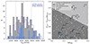 |
Fig. 1. Velocity and phase-space distributions of galaxies in Hydra I. Left panel: Distributions of the systemic velocity for galaxies in the LEWIS sample (light blue histogram), bright galaxies (mB < 16 mag, grey histogram) and dwarf galaxies (blue histogram) in Hydra I. The vertical dashed line represents the average cluster velocity (VHydra = 3683 ± 46 km s−1, from Christlein & Zabludoff 2003), and the vertical dotted lines mark the cluster velocity dispersion (σHydra = 724 ± 31 km s−1, from Lima-Dias et al. 2021). Right panel: Phase-space diagnostic diagram for galaxies in Hydra I. The systemic galaxy velocity relative to the average velocity of the cluster normalised by the cluster velocity dispersion (|Vsyst − VHydra|/σHydra) is shown as a function of the projected clustercentric distance normalised by the virial radius of the cluster (R/R200). Galaxies from the LEWIS sample are marked with light blue circles, and galaxies from Christlein & Zabludoff (2003) are marked with white dots. The black diamonds mark the objects with an irregular morphology (UDG8, UDG20, LSB4, and LSB6) described in Section 3. The shaded regions represent the very early (dark grey) and late infall or mixed times (light grey) regions (Rhee et al. 2017; Forbes et al. 2023). |
In the right panel of Figure 1, we report an updated version of the phase-space diagnostic diagram presented by Forbes et al. (2023). The systemic galaxy velocity relative to the average velocity of the cluster normalised by the cluster velocity dispersion (|Vsyst − VHydra|/σHydra) is shown as a function of the projected clustercentric distance normalised by the virial radius of the cluster (R/R200, with R200 ∼ 1.6 Mpc, Lima-Dias et al. 2021). Based on the location in phase space, we classified galaxies in the LEWIS sample into two classes: very early infall (or ancient infallers; dark grey region) and late infall or mixed times (light grey region). According to Rhee et al. (2017), the very early infallers are galaxies that entered the cluster a long time ago, and thus, they are virialised with the cluster, have lower relative velocities, and are located at smaller virial distances. Galaxies classified as late infallers/mixed times instead have higher relative velocities because they approach the cluster for the first time or have already passed the first pericenter. The majority of the galaxies in LEWIS are composed of very early infall galaxies (17) that were in the cluster for at least ∼7 Gyr (Rhee et al. 2017; Forbes et al. 2023). The remaining galaxies, classified as late infall or mixed times, might have already passed through the cluster and could be backsplash galaxies, or they did not yet enter the cluster (Table 1).
3. Structural and morphological classification
In this section, we describe the structural classification of the LEWIS galaxy sample and then provide a detailed morphological classification. We classified galaxies in the LEWIS sample into four classes according to the value of the central surface brightness μ0, g and effective radius Reff and their associated errors. According to the definition of van Dokkum et al. (2015), UDGs have Reff ≥1.5 kpc and μ0, g ≥ 24 mag arcsec−2. Classical dwarfs are brighter and more compact (with Reff < 1.5 kpc and μ0, g < 24 mag arcse−2). Compact LSB (cLSB) galaxies are fainter than classical dwarfs, but have smaller effective radii than UDGs (with Reff < 1.5 kpc and μ0,g ≥ 24 mag arcse−2). The luminosity of extended dwarf galaxies is comparable to that of dwarf galaxies, but these dwarf galaxies are more extended (with Reff ≥1.5 kpc and μ0,g < 24 mag arcse−2). We report a double classification for galaxies that are located in between two classes, taking into account the uncertainties, and we flagged galaxies as transition galaxies when they were consistent within the uncertainties with all the classes in the Reff – μ0 plane. In Table 1 we report the structural and morphological properties of the LEWIS sample derived by Iodice et al. (2020a) and La Marca et al. (2022a), as recently presented in the LEWIS Paper I (Iodice et al. 2023).
We performed an isophotal analysis on the reconstructed MUSE image of each target in the LEWIS sample. This allowed us to recover the mean geometric parameters of the galaxy and investigate their morphology. To do this, we masked all the foreground and background objects, spurious sources, GC candidates, and bad pixels in the reconstructed image. We fitted galaxy isophotes using the ELLIPSE task in the PHOTUTILS Python software (Bradley et al. 2023). First, we allowed the centre, ellipticity (ϵ), and position angle (PA) of the fitting ellipses to vary. Then, we again fitted the galaxy isophotes by fixing the centre coordinates with the median values of the x and y coordinates of the inner ellipses, and we recovered the mean PA and ϵ of the galaxy. The values are consistent with the results derived by Iodice et al. (2020b) and La Marca et al. (2022b) from VST data.
We found that the majority of the galaxies in the LEWIS sample have a regular morphology that is characterised by a nearly circular or slightly elongated shape (ϵ ∼ 0.1 − 0.3). Their light distribution is characterised by a constant core and a decrease at larger radii (see also Iodice et al. 2020a; La Marca et al. 2022b,a). We report the few cases with an irregular morphology or peculiar features below.
The UDG6 galaxy is located between the northern overdensity (La Marca et al. 2022a) and cluster centre and is characterised by an elongated shape (ϵ ∼ 0.6). By inspecting the datacube across the reconstructed image, we found several clumpy regions characterised by strong emission lines (H[[INLINE158]], [O III], H[[INLINE159]], and [S II]). Of the various targets in LEWIS, it is the UDG with the bluest colour (g − r = 0.32 ± 0.2 mag, see Iodice et al. 2020a). Due to this peculiarity, UDG6 will be studied in detail in a dedicated paper (Rossi et al., in prep.).
The UDG8 galaxy is located on the northern side of the cluster and presents an off-centred elongated structure in the inner region (Figure 4 in Appendix B, available in Zenodo). The isophotal analysis revealed a tilt of the isophotes in the inner region, characterised by a local maximum in the ellipticity profile (ϵ > 0.5) and a constant position angle (ΔPA < 10°) in the same region, which can be interpreted as a bar signature.
The UDG20 galaxy is located on the eastern side of the cluster and presents an irregular morphology (Figure 9 in Appendix B, available on Zenodo). It is characterised by two luminosity peaks, one on the north-east side, and the other on the south-west side, symmetric with respect to the geometric centre of the galaxy. We inspected these features individually by extracting a stacked spectrum of the two regions, and we found that the spectrum of the north-east region is characterised by a moderate Hα absorption line, while the spectrum of the south-west region presents a weak Hβ absorption line and a prominent Hα emission line at the same redshift as the galaxy (V ∼ 4690 km s−1). These findings suggest that these overdensities are bound to the galaxy and should be considered to be part of it.
The LSB4 galaxy is located on the northern side of the cluster and presents a disturbed morphology (Figure 13 in Appendix B, available on Zenodo). It has an elongated arc-like structure in the northern outskirts of the main body of the galaxy. This suggests that this galaxy experiences an external interaction. According to its structural parameters, this galaxy is located between the LSB and UDG regimes in the Reff − μ0 plane.
The LSB6 galaxy is located on the western side of the cluster centre and presents an elongated shape (ϵ ∼ 0.5, Figure 15 in Appendix B, available on Zenodo). The isophotes in the inner regions are characterised by a boxy shape, while in the outskirts, they are more disky. The isophotal analysis revealed a twist in the isophotes, characterised by a change in the orientation of ΔPA ∼ 10° from the inner to outer regions.
1D and 2D stellar kinematics and dynamical masses of UDGs and LSBs in the Hydra I cluster.
The UDG32 galaxy is located in the filaments of the spiral galaxy NGC 3314A. It is one of the most diffuse and faintest UDGs observed in the Hydra I cluster (μ0, g = 26 ± 1 mag arcsec−2). Its nature and location suggest that this galaxy might have originated from ram-pressure-stripped (RPS) material from NGC 3314A (Iodice et al. 2021). The MUSE data from LEWIS will allow us to understand whether this galaxy is at the same location in the cluster phase space as the stellar filaments. A detailed analysis of this interesting object is presented in Hartke et al. (2025).
The majority of the galaxies with an irregular morphology (UDG8, UDG20, and LSB6) are classified as late infall or mixed times (black diamonds, right panel of Figure 1). An isophotal twist or disrupted structures indicate possible interaction of the galaxy and cluster environment.
4. Stellar kinematics
One of the science goals of the LEWIS project is to constrain the stellar kinematics and dynamical structure of the UDGs and LSB galaxies in the Hydra I cluster. The effective velocity dispersion σeff requires a spectrum with a sufficiently high signal-to-noise ratio (S/N) to be measured. Paper I showed that the most recent version of PPXF can recover a reliable measurement of the velocity dispersion for LSB galaxies even when the value is below the actual spectral resolution of MUSE as long as the S/N of the spectrum is high enough. In particular, using Monte Carlo simulations, they demonstrated that the true value of σeff could be overestimated for spectra with S/N < 10, whereas for S/N > 15, the fitted parameters are unbiased. For this reason, we estimated the effective velocity dispersion σeff from the 1D Reff stacked spectrum, which allowed us to obtain a high S/N. The quality of the spectra, that is, the S/N, together with a precise estimate of spatial and spectral variation of the instrumental resolution are essential for accurately measuring the stellar velocity dispersion (see also Chilingarian et al. 2007). Cappellari (2017) demonstrated that with high-quality spectra (S/N > 3000 per spaxel), it is possible to recover an accurate measurement of the velocity dispersion even below the instrumental resolution. Recent papers demonstrated that in the low S/N regime as well, the values for σLOS can be derived accurately (Eftekhari et al. 2022; Iodice et al. 2023). Conversely, the derivation of the line-of-sight stellar velocity VLOS is less affected by the quality of the spectra, and thus, it is possible to relax the S/N threshold of the spectra for this measurement.
4.1. Line-of-sight velocity and effective velocity dispersion
We measured the stacked stellar kinematics of each galaxy in the LEWIS sample. We masked all possible light contamination in the FOV and defined an elliptical aperture whose centre coincided with the geometric centre of the galaxy (xc,yc), a PA and ϵ derived from the isophotal analysis, and a semi-major axis equal to Reff. We obtained the 1D stacked spectrum by co-adding all the spaxels within this elliptical aperture to derive VLOS and σeff (Figure 2, top left).
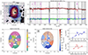 |
Fig. 2. Stacked (1D) and spatially resolved (2D) stellar kinematics of UDG1. Top left panel: MUSE-reconstructed image of UDG1. The red ellipse represents the elliptical region we used to extract the stacked spectrum within 1Reff, and the grey circles show the masked image regions. The top label reports the values of the semi-major axis (a), position angle (PA), and ellipticity (ϵ) of the ellipse. Top right panel: MUSE 1Reff stacked spectrum (solid black line) for UDG1. The bottom label reports the fit type (Table 2). The main absorption features are marked with magenta lines and labels. The solid red line represents the best-fitting spectrum obtained with PPXF. The green points show the residuals between the observed and its best-fitting spectrum. The grey areas show the masked spectral regions that we excluded from the fit. The residual points excluded from the fit are marked in blue. Bottom left panel: Voronoi-binned map of the S/N. Bottom middle panel: Stellar velocity map subtracted from the systemic velocity Vsys. The top label reports the type of rotation (Table 2). The blue and red lines mark the photometric major and minor axes of the galaxy, respectively. Bottom right panel: Velocity profiles extracted along the major (top) and minor (bottom) axes and subtracted from Vsys. |
We started by masking out all the spectral regions that were affected by contamination from the residuals of the sky-line subtraction, and we estimated the S/N of the spectrum in the spectral range used to derive the stellar kinematics (Table 2). We computed the dimensionless average S/N in the fitting wavelength range after removing the pixels that were contaminated by residuals or noisy regions and after additional filtering of the pixels through a sigma-clipping technique. The reported quantity is an average estimate, the S/N would be even higher in a restricted wavelength range around a prominent absorption line. We fitted the spectrum with the PPXF algorithm, choosing the optical wavelength range between 4800 − 7000 Å (Figure 2, top right). In a few cases, when the calcium absorption line triplet (CaT) was clearly visible, that is, when it was free from contamination of sky-line residuals, we extended the fit to 8900 Å. Since in this range MUSE reaches the best spectral resolution (FWHM ∼ 2.6 Å; see Figure A), the measured values of σeff could be more accurate. As done in Iodice et al. (2023) (see Table 2), we performed tests on different fitting spectral ranges and found consistent values of σeff within the uncertainties. We adopted the E-MILES stellar library, whose spectral resolution is similar to the average instrumental resolution, and which covers a wide range in age (from 30 Myr to 14 Gyr) and in metallicity (−2.27≤ [M/H] ≤0.4 dex). We adopted the MUSE LSF, which we measured from the sky emission lines (see Appendix A for details). As addressed in Paper I, we used additive and multiplicative Legendre polynomials to correct for discrepancies in the flux calibration and reduce imperfections in the spectral calibration that affected the continuum shape. We performed a preliminary fit by fixing the grade of additive (ADEG) and multiplicative (MDEG) polynomials to 10.
We generated 10 000 perturbations of the original spectrum by randomly removing and replacing the 30% masked spectral regions and by randomly adding 20% of the Poissonian noise without significantly varying the S/N of the perturbed spectra (on average, ΔS/N ∼1.5). We fitted the perturbed spectra by keeping VLOS fixed to the best-fitting value and adopting ADEG and MDEG Legendre polynomials as free parameters. We restricted the possible values of their polynomial degrees to the range of [0, 12] with a step of 2, also including the case of ADEG = − 1, which corresponds to not using additive polynomials. This test was made to explore different combinations for the Legendre polynomials and to determine the best combination (or a confident range of possible values) for the degrees of additive and multiplicative polynomials that ensure a reliable estimate for VLOS and σeff. The adopted interval of the degree for the additive and multiplicative polynomials ranges between 6 and 10 on average, although it is wider for highest S/N sources.
We finally fitted the 1D stacked spectrum with PPXF by fixing the grades of the additive and multiplicative polynomials to the values we obtained from the previous analysis. We estimated the errors on the fitted parameters (VLOS, σeff) by generating 1000 perturbed spectra using the same approach as explained before, and we fitted both VLOS and σeff. We estimated the associated errors by calculating the 16th and 84th percentiles of the distributions of the fitted parameters. Alternatively, the uncertainties on the fitted kinematic parameters could be estimated by using the shape of the stellar template and the information of the S/N (see Chilingarian & Grishin 2020, for details).
In Table 2 we report the S/N of the spectrum, the wavelength range used to derive the best fit, and the VLOS and σeff values for each sample galaxy.
The reliability of the fitted parameters, especially that of σeff, depends on the quality of the data. Therefore, we decided to split the sample galaxies into three types, according to the value of the average S/N of the spectrum and according to the accuracy of the final PPXF fit: 1) galaxies with a constrained fit (C), when S/N > 15 and the estimate of σeff is therefore reliable; 2) with an intermediate-quality fit (I), when 10 ≤ S/N ≤15 and the value of σeff might be slightly overestimated; 3) with an unconstrained fit (U) when the S/N < 10 and the estimate of σeff is strongly overestimated. The constrained-fit galaxies are bright objects: the S/N of all perturbed spectra is above the reliable threshold, and a broad range of ADEG and MDEG guarantees a reliable estimate of σeff. The intermediate-fit galaxies show spectra with prominent sky-line residuals in the proximity of the Hα or Hβ absorption lines that may drive the fitting algorithm to an incorrect solution. In addition, the distribution of the S/N of the perturbed spectra is broader, and the final estimate of σeff might be slightly overestimated since the spectra have S/N < 10. The unconstrained-fit galaxies are faint, and some present a disturbed morphology. Since the S/N of the extracted spectrum and the vast majority of the perturbed spectra have S/N < 10, only the value VLOS is reliable.
Figure 3 (left panel) shows the σeff distribution of the galaxies of the LEWIS sample compared to that of the UDGs studied in literature through spectroscopy (see references in Gannon et al. 2024). The light blue histogram corresponds to the galaxies with constrained fit (C in Table 2). The peak of the LEWIS sample is at σeff ∼20 − 30 km s−1, similar to that of the distribution of the literature galaxies. The majority of the values of σeff are below the actual MUSE resolution. However, all the obtained values are measured from sources with high-quality spectra (S/N > 15) with a constrained fit, and thus, the values are reliable (see also Iodice et al. 2023).
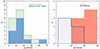 |
Fig. 3. Distributions of velocity dispersions and rotation curve semi-amplitudes of LEWIS sample. Left panel: Distributions of σeff of UDGs from literature (green histogram) and the LEWIS sample. The light blue histogram corresponds to the distribution of galaxies with a constrained fit (C-fit type). Right panel: Distribution of ΔV of UDGs in the LEWIS sample. The pink and blue histograms correspond to UDGs with a mild rotation along any axis (R and IR type) and those without rotation (NR type), respectively. |
4.2. Line-of-sight velocity field
We measured the spatially resolved stellar kinematics of each galaxy in the LEWIS sample. We masked all the foreground/background sources in the FOV and spatially binned datacube spaxels using the adaptive algorithm of Cappellari & Copin (2003) based on Voronoi tessellation to obtain a specific S/N per bin. Since we aimed to recover only the stellar velocity field, we relaxed the constraint on the threshold for the target S/N. Therefore, for each sample galaxy, we tested and adopted a different target S/N. We avoided a threshold S/N < 5, since the absorption lines were not easily visible in the stacked spectrum. In the LEWIS sample, the S/N of the stacked spectra in the Voronoi bin lies in the range S/N = 6–11 on average.
For each bin, we extracted the stacked spectrum and followed the same recipe as we adopted for the 1D case. We fitted the spectra with the PPXF algorithm, choosing the optical spectral range (4800–7000 Å) or the whole spectral range (4800–8900 Å), according to the visibility of the CaT absorption line triplet. We used the E-MILES stellar library, the LSF derived from our MUSE data, and a combination of multiplicative and additive Legendre polynomials with the same grades as we used to derive the stacked stellar kinematics, as described in the previous section. We finally reconstructed the 2D maps of the S/N and VLOS for each galaxy in the LEWIS sample (Figure 2, bottom left and centre). We adopted as systemic velocity the value obtained from the best fit of the stacked spectrum within 1Reff. After subtracting Vsys from the stellar velocity field, we derived the velocity profiles by extracting the values of VLOS in bins along apertures parallel to the photometric major and minor axes of the galaxy (Figure 2, bottom right).
Unfortunately, we were not able to derive the spatially resolved stellar kinematics for all the targets. Two galaxies were extremely faint, and the application of the Voronoi binning returned a single bin (i.e. UDG13 and UDG15). In some other cases, the application of the Voronoi algorithm returned only two bins that split the galaxy into two nearly symmetric halves (i.e. UDG3, UDG20, UDG21, UDG23, LSB1, and LSB4). For these galaxies, we lack enough data points to properly extract a velocity profile, and we therefore flagged these targets with U (unconstrained) in Table 2. The 2D velocity maps derived for all the LEWIS targets, including the unconstrained cases, are shown in Appendix B (available on Zenodo). As already pointed out in Section 3, UDG6 and UDG32 are two special cases that will be analysed and presented in detail in dedicated papers (Rossi et al., in prep., Hartke et al. 2025).
5. Results
In this section, we present the stellar kinematics properties and constraints on the dynamical mass and DM content of the LEWIS sample based on the stellar kinematics derived from the MUSE data, and we compare the results with the data published in the literature.
5.1. Stellar velocity profiles
We evaluated the stellar kinematics of the galaxy sample. We computed the semi-amplitude of the rotation curve (ΔV) as the semi-difference of the first and last point of the velocity profile along the kinematic major axis. We found that galaxies in the LEWIS sample span a wide range of kinematic features. Thus, we decided to classify them into three classes as described below.
-
Rotation along the major photometric axis (R): Some galaxies show mild rotation along the major photometric axis (UDG1, UDG7, and LSB6) with values ΔV ∼ 25 − 40 km s−1. We found that the central regions of the velocity profile appear to have mild variations in terms of velocity on average; the values can also be consistent with Vsys. In the outskirts, the velocity instead reaches opposite values on the two sides, and the values are not compatible with Vsys even considering their uncertainties. These galaxies are flagged with R in Table 2.
-
Rotation along an intermediate axis (IR): A few UDGs in the LEWIS sample show mild rotation along a different axis than the major photometric one (UDG8, UDG12, LSB7, and LSB8). In these cases, we plot the velocity profile along this direction in an additional panel (e.g. green line in Figure 4 in Appendix B, available on Zenodo), and we report the corresponding value of ΔV. Some of these objects have a roundish shape (ϵ < 0.3), and it might thus be possible that this simple morphology hides a more complex internal dynamical structure. These galaxies are flagged with IR in Table 2.
-
No rotation (NR): Other UDGs do not show clear evidence of rotation in any direction (UDG4, UDG9, UDG11, and LSB5). The velocity profiles along the major, minor, or intermediate axis do not show a clear velocity difference between the two sides. In addition, some velocity values have large uncertainties that are consistent with Vsys. These galaxies are flagged with NR in Table 2.
The values for ΔV are measured on the sky-plane and are reported in Table 2.
We stress that the classification of the kinematic feature is based on the presence of a significant velocity difference along a certain axis. Due to the extremely faint nature of UDGs and the effectiveness of the MUSE data, the derived VLOS map does not extend beyond the Reff of the galaxy for most targets. Furthermore, in some cases, the detection of a velocity difference might be induced by an external tidal distortion rather than by internal stellar kinematics. These events might affect the morphology (e.g. LSB4 and LSB6) or produce kinematic signals along different axes (see also Łokas 2024).
Figure 3 (right panel) shows the distribution of ΔV for UDGs in LEWIS. The pink and blue histograms correspond to the UDGs with mild rotation along any axis (R and IR type) and those without clear rotation (NR type), respectively. The majority of the galaxies in the sample (7 out of 18) show rotation with values of ΔV ∼ 30 − 40 km s−1.
5.2. The Faber-Jackson relation
In Figure 4 (left panel) we show the effective velocity dispersion σeff as a function of stellar masses (M*) of galaxies from the LEWIS sample and the literature (see references in Gannon et al. 2024). As noted in Section 4.1, for galaxies with an intermediate and an unconstrained fit (I and U fit types, respectively), the values of σeff and thus all the derived quantities are overestimated. In the forthcoming analysis, we excluded these cases before we drew our final considerations. The stellar masses were estimated by Iodice et al. (2020a) and La Marca et al. (2022a) using galaxy luminosities and the Into & Portinari (2013) colour – M/L relation.
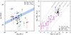 |
Fig. 4. Faber-Jackson relation and dark matter content in LEWIS sample. Left panel: Velocity dispersion σeff as a function of stellar masses of UDGs from the literature (green diamonds) and the LEWIS sample. The blue and red circles represent rotating and non-rotating LEWIS galaxies, respectively. The shaded light blue region represents the luminosity Faber-Jackson relation, extrapolated to the low-mass regime (L ∼ σ2.2, Kourkchi et al. 2012). The luminosities are converted into stellar masses using the Into & Portinari (2013) colour – M/L relation. UDG7 and UDG12 are marked with triangles since their values of σeff might be overestimated due to their non-negligible rotation. Right panel: Dynamical mass (Mdyn) as a function of the V-band total luminosity (LV, eff) computed within 1Reff of UDGs from the literature (green diamonds) and the LEWIS sample. The points are colour-coded as in the left panel. The solid grey lines mark the loci in the plane where Mdyn/LV, eff is constant and equal to 1, 10, 100, 1000, and 10 000, respectively. The magenta points represent the dwarf galaxies in the Local Group analysed by Battaglia & Nipoti (2022). |
We identified three groups of objects in the M* − σeff plane. A group of UDGs (6 out of 11) are consistent within the uncertainties with the prediction of the Faber-Jackson relation extrapolated to the low-mass regime (L ∼ σ2.2, Kourkchi et al. 2012). For two objects, σeff is higher than predicted (UDG7 and UDG12). These UDGs have a non-negligible rotation velocity (ΔV ∼ 30 − 40 km s−1), and thus, their values of σeff might be contaminated by the contribution of rotation (see also Section 5.3). A few galaxies are instead below the prediction of the Faber-Jackson relation (LSB7 and LSB8). They have a non-negligible rotation velocity (i.e. ΔV ∼ 20 − 25 km s−1). UDG4 is another outlier of the Faber-Jackson relation. It is a genuine UDG without any indication of rotation along any axis. Despite its position in the M* − σeff plane and the large scatter, it is consistent with other UDGs from the literature.
5.3. Dark matter content
To constrain the DM content, we computed the dynamical mass (Mdyn) by applying the formula proposed in Wolf et al. (2010): Mdyn = 4Reff, c σeff2/G, where Reff, c = Reff is the circularised half-light radius calculated through the galaxy axial ratio q, and G is the gravitational constant. Thus, Mdyn is the mass enclosed in a sphere with the radius of a circularised deprojected half-light radius. The Wolf et al. (2010) formula was widely applied in many literature works and is valid for dispersion-supported systems.
Nevertheless, we found that the rotation amplitude for a significant fraction of galaxies in LEWIS is comparable to the value for σeff (ΔV≳ σeff), and thus, they cannot be considered dispersion-supported systems. With some variation, the formula proposed in Wolf et al. (2010) can be used to derive a good estimate for the enclosed mass in any case. As described in Courteau et al. (2014), σeff in real galaxies does not correspond to the stellar velocity dispersion, but can be considered as an approximation of the luminosity-weighted second velocity moment (σeff2 ≈ ⟨Vrms2⟩=⟨V2 + σ2⟩), with V and σ the observed mean stellar velocity and the corresponding dispersion, respectively. Thus, it already includes the rotation and velocity dispersion of the stars and is sometimes erroneously termed σ.
We tested whether the approximation provided in Courteau et al. (2014) is still valid for the class of rotating UDGs to investigate the effect on the dynamical masses. To do this, we decided to repeat the extraction of the stellar kinematics to measure VLOS and σLOS. However, to obtain an unbiased estimate of σLOS, we required that all the spectra of the Voronoi bins had a sufficiently high S/N ≳ 15. This was the case for five out of the seven rotating galaxies in LEWIS. For these galaxies, we extracted a map of the σLOS (see Appendix C, available on Zenodo), and we were able to compute an independent measure of the effective velocity dispersion by averaging the σLOS values in the various bins within an elliptical aperture with semi-major axis a = Reff. The values of σeff are slightly lower than the estimate provided by the 1D stacked spectrum. Finally, we computed the luminosity-weighted second velocity moment Vrms and calculated the dynamical mass using Vrms. For UDG7, UDG12, and galaxies without clear rotation (NR-type), we computed the dynamical mass from σeff.
We calculated the V-band total luminosity in the (LV, eff) after converting the r-band magnitude using the formula proposed in Kostov & Bonev (2018). In this way, we computed the dynamical mass-to-light ratio (Mdyn/LV, eff) and evaluated the amount of baryonic and DM content bound to the system. The values for Mdyn and Mdyn/LV, eff are reported in Table 2.
In Figure 4 (right panel) we show Mdyn as a function of the total luminosity in V band of galaxies from the LEWIS sample and the literature (Gannon et al. 2024). In addition, we plot the catalogue of dwarf galaxies in the Local Group studied by Battaglia & Nipoti (2022). The grey lines mark the loci where Mdyn/LV, eff is constant and equal to 1, 10, 100, 1000, and 10 000, respectively. The majority of galaxies in the LEWIS sample have a DM content that exceeds that of the Local Group dwarf galaxies with a similar total luminosity (Mdyn/LV, eff ∼ 10–100 M⊙/L⊙), as found in previous works (Gannon et al. 2021). Galaxies taken from Battaglia & Nipoti (2022) are dwarf galaxies in the Local Group, that is, they are located at a distance D < 1 Mpc from the Milky Way. Their internal dynamics were investigated by using the spatially resolved kinematics of individual stars. The values of σeff inferred for these objects rely on precise measurements of the stellar velocities, whereas the values of σeff for the galaxies in the LEWIS sample were estimated by measuring the global stellar motions along the line of sight. With LEWIS, an additional constraint on the DM content can be provided by analysing the GC dynamics (Mirabile et al., in prep.).
Two objects, UDG7 and UDG12, have an exceptionally high value of the effective velocity dispersion, which is σeff = 61 ± 9 km s−1 and σeff = 38 ± 9 km s−1, respectively. These UDGs are characterised by mild rotation along the photometric major axis (ΔV ∼ 30 − 40 km s−1), and thus, the values of σeff can be contaminated by the contribution of rotation. These are the two UDGs for which we were unable to derive the σLOS field and thus Vrms. We estimated the derived quantities using σeff in any case. The values of Mdyn and Mdyn/LV, eff can be overestimated by one order of magnitude. We flagged UDG7 and UDG12 in Table 2.
5.4. Kinematic support of the LEWIS galaxies
We extracted the VLOS and σLOS maps for the five galaxies of the LEWIS sample with a sufficiently high S/N (UDG1, UDG8, LSB6, LSB7, and LSB8). For these galaxies, we provide information on the kinematic support by calculating the projected specific angular momentum (λR), which is defined as
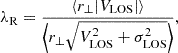
where r⊥ is the projected distance of the bin to the centre of the galaxy, and ⟨ ⟩ represents the flux-weighted average over the galaxy image (Emsellem et al. 2011). This quantity requires a 2D stellar kinematics map and accurate measurements of σLOS, and it is a diagnostic of the kinematic support. According to this parameter, high values of λR correspond to rotation-supported galaxies, that is, the kinematic structure is characterised by ordered rotational motion. On the other hand, low values for λR correspond to a dispersion-supported system, that is, the kinematic structure is characterised by random motions.
In Figure 5 we show λR as a function of galaxy ellipticity ϵ (left panel) and stellar mass (right panel). The black curve in the left panel ( splits the galaxies in rotation-supported (above the line) and dispersion-supported (below the line) systems (Emsellem et al. 2011). Light blue circles represent the LEWIS galaxies, while pink squares represent the dwarf ellipticals from Scott et al. (2020). This sample is composed of dwarf galaxies that belong to the Virgo cluster of galaxies (D ∼ 20 Mpc), which are morphologically classified as ellipticals (dE) or lenticulars (dS0), with an effective r-band surface brightness between 18 < μr < 24 mag arcsec−2 and stellar masses between 108 < M* < 109.5 M⊙. With a similar approach, the authors applied on their datacubes the Voronoi binning algorithm with an S/N = 10 to derive the mean VLOS and σLOS and thus retrieved the kinematic support of the galaxies by computing the relative angular momentum, that is, the λR parameter. They found that values of λR in dwarf galaxies span a wide range (∼0.1 − 0.4) on average and reported a mild correlation between the kinematic support and stellar mass. Combining their catalogue of dwarf galaxies with several catalogues of bright and massive galaxies, Scott et al. (2020) claimed that λR reaches a maximum around M* ∼ 1010 M⊙ and decreases towards the low- and very-high-mass regimes. The LEWIS galaxies span a wide range of ϵ and are characterised by values 0.25 ≲ λR ≲ 0.35. We found no distinction between the two UDGs and the three LSB galaxies.
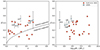 |
Fig. 5. Kinematic support in LEWIS sample. Projected specific angular momentum (λR) as a function of galaxy ellipticity (left panel) and stellar mass (right panel). The light blue circles mark the LEWIS galaxies, and the pink squares represent the dwarf galaxies studied by Scott et al. (2020). The black curve in the left panel ( |

6. Discussion: Two kinematical classes of UDGs in the Hydra I cluster
Based on the 2D stellar kinematics, we claim that the LSB galaxies and UDGs in the Hydra I cluster can be grouped into two classes on average: galaxies that rotate mildly, and galaxies without rotation along any axis.
We find a narrow distribution for σeff in the LEWIS galaxies. The majority of UDGs and LSB galaxies have a similar DM content (Mdyn/LV, eff ∼ 10–100 M⊙/L⊙), which is higher than that observed in dwarf galaxies with a comparable luminosity.
The main result of the paper is that the galaxies have different kinematical types. This suggests different formation pathways for UDGs and LSB galaxies in the Hydra I cluster. Because they are extremely faint, systematic studies of the kinematic support of UDGs are unfortunately lacking in the literature. Only a few theoretical works provided predictions for the stellar kinematics.
Cardona-Barrero et al. (2020) studied the kinematic support of isolated UDGs in NIHAO simulations (Wang et al. 2015). The authors found that UDGs span a continuous distribution of λR values for different inclination angles from 0° up to 90°. In particular, for galaxies with an inclination between 30° to 60°, λR varies from 0.2 to 0.7. These values are consistent with those derived for the LEWIS rotating galaxies, which have similar inclinations, and 0.25 ≤ λR ≤ 0.35 (Figure 5). The LEWIS galaxies are located in a cluster environment, but Cardona-Barrero et al. (2020) explored the kinematical properties of field UDGs.
In addition, Cardona-Barrero et al. (2020) found no correlation of λR with stellar mass, but they found correlations with the morphological properties, HI gas content, and size. Larger UDGs are more rotation-supported, have a high HI gas content and present a disk-like morphology. In contrast, dispersion-supported UDGs have a low HI gas content and resemble triaxial spheroids. The kinematic prediction suggests that the isolated UDGs in NIHAO simulations formed due to intense gas outflow.
Benavides et al. (2023) adopted a similar approach to studying UDGs in broader environmental conditions in TNG50 simulations. They did not measure λR, but they considered the ratio of the rotational support and total kinematic energy of the galaxy. This quantity cannot be measured in real observations since it relies on quantities that are related to stellar particles. However, it allows us to distinguish rotation and dispersion-supported systems, similarly to the λR parameter. Benavides et al. (2023) found no differences in terms of kinematic support between field UDGs and UDGs in most dense regions, suggesting that the environmental effects act more quickly on the stellar distribution than on the internal dynamics. This result might agree with comparable values of λR for the field UDGs by Cardona-Barrero et al. (2020) and for our LEWIS galaxies in the Hydra I cluster.
In addition, Benavides et al. (2023) found a correlation between the kinematic support and stellar mass, which indicates that more massive UDGs (M* ≳ 108.5 M⊙) are more strongly supported by rotation and have a disk-like morphology. Since this trend was also found in populations of non-UDGs, they wondered whether this might be due to a specific parametrisation of the baryonic modelling in TNG50 simulations, or if it is a peculiarity of the class of UDGs. As in Benavides et al. (2023), we find a mild trend of the rotational support with increasing mass (Figure 5, right panel), but more systematic studies are required to address and confirm the kinematic support in UDGs.
The distinction into two classes of UDGs proposed by Sales et al. (2020) is based on the distributions of the effective velocity dispersion and metallicity, but no indication of the stellar rotation is provided. Therefore, no comparison between the observed stellar kinematics of LEWIS galaxies and this set of simulations can be made.
6.1. Correlations within the cluster environment
In Figure 6 we show the stellar mass (left panel), σeff (middle panel) and Mdyn/LV, eff (right panel) as a function of the cluster-centric distance5. In these plots, we mark the innermost regions of the cluster that are dominated by the X-ray emission, which corresponds to R ∼ 14 arcmin (Spavone et al. 2024).
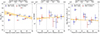 |
Fig. 6. Correlations between structural properties and cluster environment. Left panel: Stellar mass as a function of the cluster-centric distance. Middle panel: σeff as a function of the cluster-centric distance. Right panel: Dynamical mass-to-light ratio Mdyn/LV, eff as a function of the cluster-centric distance. The vertical dashed grey line marks the radial distance within which the X-ray emission of the cD galaxy dominates (14 arcmin, Spavone et al. 2024). The labels identify the LEWIS galaxies. Filled circles represent galaxies classified as very early infall, and empty circles represent galaxies classified as late infall or mixed times. The blue and red circles represent rotating and non-rotating galaxies, respectively. The yellow line represents a linear fit obtained by excluding the values for UDG7 and UDG12. The uncertainties on the fitting lines were computed using a bootstrap technique. In the central and right panels, UDG7 and UDG12 are marked with triangles since their values of σeff and Mdyn/LV, eff might be overestimated due to their non-negligible rotation. |
We performed a linear fit to data and their uncertainties to highlight possible correlations between the derived properties and the position in the cluster. We considered both early and late infallers. They are cluster members according to their Vsys despite their location in the phase-space diagram. Since the Mdyn values for UDG7 and UDG12 are overestimated due to a non-negligible contribution of the rotation velocity, we discarded them from the fit. We found a weak trend of the stellar mass with the cluster-centric distance, where more massive UDGs are close to the centre. The values of the stellar masses will be derived independently from the analysis of the stellar population (Doll et al., in prep.), and thus, an updated version of this figure will be shown in a forthcoming paper. We found a mild trend of σeff with the cluster-centric distance, where galaxies with lower values of σeff are located in the inner regions. An opposite, but also weak, correlation appears in the log10(Mdyn/LV, eff) – distance plane, suggesting that DM-dominated galaxies are located at smaller distances from the cluster core.
According to the predictions by Sales et al. (2020), T-UDGs populate the centre of the clusters, and at a given stellar mass, they have a lower σeff, a higher metallicity, and a lower DM fraction than the B-UDG. Since we found a significant fraction of galaxies with non-negligible rotation, we cannot directly compare our findings with the results provided in Sales et al. (2020). They assumed that UDGs are dispersion-supported systems to estimate σeff. Our rotating UDGs cannot be considered dispersion-supported systems, and thus, the estimate of σeff is affected by the rotation and is not representative of the true stellar velocity dispersion. In addition, taking into account that the LEWIS sample is located within 0.4R200, our analysis is mainly focused on the innermost regions of the Hydra I cluster.
In Figure 7 we show the semi-amplitude of the velocity profile ΔV as a function of the cluster-centric distance. In this plot, we colour-code the data points according to the values of the Reff (left panel), colour g − r (central panel), and σeff (right panel). In this way, we tested for a correlation of the dynamical and structural properties of the UDG and LSB galaxies in the Hydra I cluster.
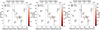 |
Fig. 7. Correlations between kinematic properties and cluster environment. Semi-amplitude of the rotation curve ΔV as a function of the cluster-centric distance. The data points are colour-coded according to the values of the Reff (left panel), colour g − r (central panel), and σeff (right panel). As in Figure 6, the vertical dashed line marks the extension of the X-ray emission. The circles represent galaxies that rotate along the photometric major axis or intermediate axis (R and IR-type), and triangles show galaxies without rotation (NR-type). |
If galaxies have a disk-like memory of their past evolutionary pathway, we might expect higher values of ΔV and Reff, lower values of σeff and bluer g − r colours because galaxies with disk morphology/dynamics are expected to have younger stellar populations with more ordered motions. We found no clear trend considering the different explored quantities or concerning the projected cluster-centric distance. In particular, UDGs and LSB galaxies with rotation are found at any distance from the core of the cluster.
7. Summary and concluding remarks
We performed a kinematic analysis for a homogeneous and almost a complete sample of UDG and LSB galaxies in the Hydra I cluster of galaxies with MUSE data from the LEWIS project (Iodice et al. 2023). The observing campaign is complete to ∼92%, and we were able to provide values of Vsys for more objects than in the first release (Paper I). We found that the systemic velocities of nearly all LEWIS targets are consistent with the overall velocity distribution of the giant and dwarf galaxy populations in the cluster (Figure 1). In particular, 15 out of 23 objects have Vsys within 1σHydra. The remaining 8 galaxies have a higher relative Vsys, but within 2σHydra.
This paper focused on the stellar kinematics of the LEWIS targets to derive the rotation velocity and velocity dispersion. Based on the IF nature of the LEWIS data, we were able to derive 2D velocity maps for most of the sample galaxies. This represents the first large sample of 2D stellar velocity maps for UDG and LSB galaxies. A stellar velocity field was extracted before only for UDG NGC 1052-DF2 and DF44. NGC 1052-DF2 shows mild rotation with ΔV ∼ 6 km s−1, and DF 44 shows no evidence of rotation (Emsellem et al. 2019; van Dokkum et al. 2019).
The main results are summarised below.
-
The peak of the distribution of σeff ranges between 20 and 30 km s−1, which is consistent with the distribution of the values from the literature data (Figure 3, left panel). Two LSB galaxies in the sample have extremely low values of σeff (σeff ≤15 km s−1) and two UDGs have very high values of σeff (σeff ≥40 km s−1). These sources have high-quality spectra (S/N > 15), and the estimate of their σeff is therefore reliable.
-
Based on the 2D map of the stellar velocity, 7 out of 18 LEWIS galaxies show a mild rotation (ΔV ∼ 25–40 km s−1). The rotation of 3 of them is along the photometric major axis, and for the other 4, it is along an intermediate axis. Five LEWIS galaxies do not show evidence of rotation, and for the remaining 6, our results are unconstrained (Figure 3, right panel)
-
Compared to the Faber-Jackson relation, we found three groups of UDGs. A group of UDGs in Hydra I is consistent with the relation extrapolated to the low-mass regime, that is, L ∼ σ2.2 (Kourkchi et al. 2012). A few galaxies are outliers of the Faber-Jackson relation. UDG7 and UDG12 have higher values of σeff than expected for their stellar mass. These values are overestimated due to a non-negligible contribution of the rotation. UDG4, LSB7, and LSB8 instead have values for σeff below the relation (Figure 4, left panel).
-
The majority of the galaxies of the LEWIS sample (i.e. both the UDGs and LSB galaxies) have a higher DM content than dwarf galaxies with a similar total luminosity Mdyn/LV, eff ∼ 10–100 M⊙/L⊙ (Figure 4, right panel).
-
For five of the seven rotating galaxies in LEWIS, we derived the λR parameter, which is a diagnostic of the kinematic support. They are characterised by values 0.25 ≲ λR ≲ 0.35, suggesting that these galaxies are rotation supported. We found no distinction between UDGs and LSBs (see Figure 5).
Considering the enormous technical and observational challenge of obtaining spectra for LSB galaxies, whose surface brightness is only a small fraction of the sky level, the results from LEWIS showed that the combination of the large collecting area of the Very Large Telescopes and the high efficiency of the MUSE IF spectrograph truly paved the way for the spectroscopic characterisation of this class of faint objects.
We provided an extended census of the stellar kinematics for UDGs in a cluster environment. In particular, we reported for the first time a considerable number of UDGs and LSB galaxies that are supported by rotation. These results indicate two kinematical classes of UDGs in the Hydra I cluster, and the classes might have different origins.
However, the stellar kinematic properties are not sufficient to distinguish between the formation channels that were proposed by theoretical works on UDGs. Stringent constraints on any possible relation with the environment in which UDGs reside can be obtained by combining the stellar kinematics with other UDG properties. The stellar population analysis and GC content will be investigated with the LEWIS data and presented in forthcoming papers of the LEWIS series (Doll et al., in prep., Mirabile et al., in prep.). Iodice et al. (2023) have already demonstrated that LEWIS will enable us to confirm GCs that were pre-selected through photometry, to spectroscopically identify new GC systems, and to study their stellar kinematics and population.
The results presented in this paper also opened a new topic to be investigated for UDGs. Upcoming works will focus on the analysis of the available cosmological simulations to extract the missing information on the stellar kinematics, to be compared with results derived from MUSE data for the UDGs in the Hydra I cluster. This type of analysis would also trigger additional interest in IF spectroscopic data for this class of galaxies.
Data availability
The data underlying this article (in the Appendix B and C) are made available on Zenodo: https://doi.org/10.5281/zenodo.14747456
https://sites.google.com/inaf.it/lewis/home
SKYFR_1 and SKYFR_2 are the fraction of spaxels in the sky image and scientific image used to evaluate the sky background, respectively.
CFWIDTHSP is the window size for the continuum filter used to remove the continuum features for calculating the eigenvalues per spectrum.
CFWIDTHSVD is the window size for the continuum filter for the SVD computation.
Consistently with Forbes et al. (2023), we assumed RA = 159.17842, Dec = − 27.528339 as the centre of the Hydra I cluster, which corresponds to the centre of the bright cluster member NGC 3311.
Acknowledgments
We wish to thank the anonymous Referee whose comments helped us to improve the clarity of the manuscript. Based on observations collected at the European Southern Observatory under ESO programmes 108.222P.001, 108.222P.002, 108.222P.003. The authors wish to thank L. Buzzo, L. Coccato, V. Debattista, E. Emsellem, A. Ferre-Mateu, J. Gannon, L. Greggio, F. Marleau, O. Muller, T. Puzia, R. Rampazzo for the useful comments and discussions on the work presented in this paper. E.I. acknowledges support by the INAF GO funding grant 2022-2023. E.I., E.M.C. and M.P. acknowledge the support by the Italian Ministry for Education University and Research (MIUR) grant PRIN 2022 2022383WFT “SUNRISE”, CUP C53D23000850006. J.H. and E.I. acknowledge the financial support from the visitor and mobility programme of the Finnish Centre for Astronomy with ESO (FINCA), funded by the Academy of Finland grant nr 306531. J.H. wishes to acknowledge CSC-IT Center for Science, Finland, for computational resources. E.M.C. acknowledges the support from MIUR grant PRIN 2017 20173ML3WW-001 and Padua University grants DOR 2021-2023. G.D. acknowledges support by UKRI-STFC grants: ST/T003081/1 and ST/X001857/1. D.F. thanks the ARC for support via DP220101863 and DP200102574. J.F-B. acknowledges support from the PID2022-140869NB-I00 grant from the Spanish Ministry of Science and Innovation. This work is based on the funding from the INAF through the GO large grant in 2022, to support the LEWIS data reduction and analysis (PI E. Iodice). The authors thank Gannon et al. (2024) for the compilation of their catalogue of UDG spectroscopic properties. The catalogue includes data from: McConnachie (2012), van Dokkum et al. (2015, 2016, 2017, 2018, 2019), Beasley et al. (2016), Martin et al. (2016, 2019), Yagi et al. (2016), Martínez-Delgado et al. (2016), Karachentsev et al. (2017), Toloba et al. (2018, 2023), Gu et al. (2018), Lim et al. (2018, Lim et al. (2020, Ruiz-Lara et al. (2018), Alabi et al. (2018), Ferré-Mateu et al. (2018), Ferré-Mateu et al. (2023), Forbes et al. (2018, 2021), Chilingarian et al. (2019), Fensch et al. (2019), Danieli et al. (2019), 2022), Torrealba et al. (2019), Iodice et al. (2020a), Collins et al. (2020), Müller et al. (2020, 2021), Gannon et al. (2020, 2021, 2022, 2023), Shen et al. (2021, 2023), Ji et al. (2021), Huang & Koposov (2021), Mihos et al. (2022), Villaume et al. (2022), Webb et al. (2022), Saifollahi et al. (2022), Janssens et al. (2022). The authors acknowledge the use of the following Python scripts: ASTROPY (Astropy Collaboration 2013, 2018), MATPLOTLIB (Hunter 2007), MPDAF (Bacon et al. 2016), NUMPY (van der Walt et al. 2011), PHOTUTILS (Bradley et al. 2023), SCIPY (Virtanen et al. 2020), and ZAP (Soto et al. 2016).
References
- Alabi, A., Ferré-Mateu, A., Romanowsky, A. J., et al. 2018, MNRAS, 479, 3308 [Google Scholar]
- Alabi, A. B., Romanowsky, A. J., Forbes, D. A., Brodie, J. P., & Okabe, N. 2020, MNRAS, 496, 3182 [NASA ADS] [CrossRef] [Google Scholar]
- Amorisco, N. C., & Loeb, A. 2016, MNRAS, 459, L51 [NASA ADS] [CrossRef] [Google Scholar]
- Arnaboldi, M., Ventimiglia, G., Iodice, E., Gerhard, O., & Coccato, L. 2012, A&A, 545, A37 [NASA ADS] [CrossRef] [EDP Sciences] [Google Scholar]
- Astropy Collaboration (Robitaille, T. P., et al.) 2013, A&A, 558, A33 [NASA ADS] [CrossRef] [EDP Sciences] [Google Scholar]
- Astropy Collaboration (Price-Whelan, A. M., et al.) 2018, AJ, 156, 123 [Google Scholar]
- Bacon, R., Accardo, M., Adjali, L., et al. 2010, in Ground-based and Airborne Instrumentation for Astronomy III, Proc. SPIE, 7735, 773508 [Google Scholar]
- Bacon, R., Piqueras, L., Conseil, S., Richard, J., & Shepherd, M. 2016, Astrophysics Source Code Library [record ascl:1611.003] [Google Scholar]
- Bacon, R., Conseil, S., Mary, D., et al. 2017, A&A, 608, A1 [NASA ADS] [CrossRef] [EDP Sciences] [Google Scholar]
- Battaglia, G., & Nipoti, C. 2022, Nat. Astron., 6, 1492 [NASA ADS] [CrossRef] [Google Scholar]
- Beasley, M. A., Romanowsky, A. J., Pota, V., et al. 2016, ApJ, 819, L20 [NASA ADS] [CrossRef] [Google Scholar]
- Benavides, J. A., Sales, L. V., Abadi, M. G., et al. 2023, MNRAS, 522, 1033 [NASA ADS] [CrossRef] [Google Scholar]
- Bennet, P., Sand, D. J., Zaritsky, D., et al. 2018, ApJ, 866, L11 [NASA ADS] [CrossRef] [Google Scholar]
- Bradley, L., Sipőcz, B., Robitaille, T., et al. 2023, https://doi.org/10.5281/zenodo.7946442 [Google Scholar]
- Buzzo, M. L., Forbes, D. A., Brodie, J. P., et al. 2022, MNRAS, 517, 2231 [NASA ADS] [CrossRef] [Google Scholar]
- Buzzo, M. L., Forbes, D. A., Jarrett, T. H., et al. 2024, MNRAS, 529, 3210 [NASA ADS] [CrossRef] [Google Scholar]
- Cappellari, M. 2017, MNRAS, 466, 798 [Google Scholar]
- Cappellari, M., & Copin, Y. 2003, MNRAS, 342, 345 [Google Scholar]
- Cappellari, M., & Emsellem, E. 2004, PASP, 116, 138 [Google Scholar]
- Cardona-Barrero, S., Di Cintio, A., Brook, C. B. A., et al. 2020, MNRAS, 497, 4282 [NASA ADS] [CrossRef] [Google Scholar]
- Carleton, T., Guo, Y., Munshi, F., Tremmel, M., & Wright, A. 2021, MNRAS, 502, 398 [NASA ADS] [CrossRef] [Google Scholar]
- Chilingarian, I. V., & Grishin, K. A. 2020, PASP, 132, 064503 [NASA ADS] [CrossRef] [Google Scholar]
- Chilingarian, I. V., Prugniel, P., Sil’Chenko, O. K., & Afanasiev, V. L. 2007, MNRAS, 376, 1033 [NASA ADS] [CrossRef] [Google Scholar]
- Chilingarian, I. V., Afanasiev, A. V., Grishin, K. A., Fabricant, D., & Moran, S. 2019, ApJ, 884, 79 [NASA ADS] [CrossRef] [Google Scholar]
- Christlein, D., & Zabludoff, A. I. 2003, ApJ, 591, 764 [Google Scholar]
- Collins, M. L. M., Tollerud, E. J., Rich, R. M., et al. 2020, MNRAS, 491, 3496 [NASA ADS] [CrossRef] [Google Scholar]
- Collins, M. L. M., Read, J. I., Ibata, R. A., et al. 2021, MNRAS, 505, 5686 [NASA ADS] [CrossRef] [Google Scholar]
- Courteau, S., Cappellari, M., de Jong, R. S., et al. 2014, Rev. Mod. Phys., 86, 47 [Google Scholar]
- Danieli, S., van Dokkum, P., Conroy, C., Abraham, R., & Romanowsky, A. J. 2019, ApJ, 874, L12 [NASA ADS] [CrossRef] [Google Scholar]
- Danieli, S., van Dokkum, P., Trujillo-Gomez, S., et al. 2022, ApJ, 927, L28 [NASA ADS] [CrossRef] [Google Scholar]
- Di Cintio, A., Brook, C. B., Dutton, A. A., et al. 2017, MNRAS, 466, L1 [NASA ADS] [CrossRef] [Google Scholar]
- Eftekhari, F. S., Peletier, R. F., Scott, N., et al. 2022, MNRAS, 517, 4714 [NASA ADS] [CrossRef] [Google Scholar]
- Emsellem, E., Cappellari, M., Krajnović, D., et al. 2007, MNRAS, 379, 401 [Google Scholar]
- Emsellem, E., Cappellari, M., Krajnović, D., et al. 2011, MNRAS, 414, 888 [Google Scholar]
- Emsellem, E., van der Burg, R. F. J., Fensch, J., et al. 2019, A&A, 625, A76 [NASA ADS] [CrossRef] [EDP Sciences] [Google Scholar]
- Falcón-Barroso, J., Sánchez-Blázquez, P., Vazdekis, A., et al. 2011, A&A, 532, A95 [Google Scholar]
- Fensch, J., van der Burg, R. F. J., Jeřábková, T., et al. 2019, A&A, 625, A77 [NASA ADS] [CrossRef] [EDP Sciences] [Google Scholar]
- Ferré-Mateu, A., Alabi, A., Forbes, D. A., et al. 2018, MNRAS, 479, 4891 [CrossRef] [Google Scholar]
- Ferré-Mateu, A., Gannon, J. S., Forbes, D. A., et al. 2023, MNRAS, 526, 4735 [CrossRef] [Google Scholar]
- Forbes, D. A., Read, J. I., Gieles, M., & Collins, M. L. M. 2018, MNRAS, 481, 5592 [NASA ADS] [CrossRef] [Google Scholar]
- Forbes, D. A., Alabi, A., Romanowsky, A. J., Brodie, J. P., & Arimoto, N. 2020, MNRAS, 492, 4874 [Google Scholar]
- Forbes, D. A., Gannon, J. S., Romanowsky, A. J., et al. 2021, MNRAS, 500, 1279 [Google Scholar]
- Forbes, D. A., Gannon, J., Iodice, E., et al. 2023, MNRAS, 525, L93 [NASA ADS] [CrossRef] [Google Scholar]
- Freudling, W., Romaniello, M., Bramich, D. M., et al. 2013, A&A, 559, A96 [NASA ADS] [CrossRef] [EDP Sciences] [Google Scholar]
- Gannon, J. S., Forbes, D. A., Romanowsky, A. J., et al. 2020, MNRAS, 495, 2582 [NASA ADS] [CrossRef] [Google Scholar]
- Gannon, J. S., Dullo, B. T., Forbes, D. A., et al. 2021, MNRAS, 502, 3144 [Google Scholar]
- Gannon, J. S., Forbes, D. A., Romanowsky, A. J., et al. 2022, MNRAS, 510, 946 [Google Scholar]
- Gannon, J. S., Forbes, D. A., Brodie, J. P., et al. 2023, MNRAS, 518, 3653 [Google Scholar]
- Gannon, J. S., Ferré-Mateu, A., Forbes, D. A., et al. 2024, MNRAS, 531, 1856 [NASA ADS] [CrossRef] [Google Scholar]
- Gu, M., Conroy, C., Law, D., et al. 2018, ApJ, 859, 37 [Google Scholar]
- Hartke, J., Iodice, E., Gullieuszik, M., et al. 2025, A&A, submitted [arXiv:2501.16192] [Google Scholar]
- Huang, K.-W., & Koposov, S. E. 2021, MNRAS, 500, 986 [Google Scholar]
- Hunter, J. D. 2007, Comput. Sci. Eng., 9, 90 [NASA ADS] [CrossRef] [Google Scholar]
- Into, T., & Portinari, L. 2013, MNRAS, 430, 2715 [Google Scholar]
- Iodice, E., Cantiello, M., Hilker, M., et al. 2020a, A&A, 642, A48 [EDP Sciences] [Google Scholar]
- Iodice, E., Spavone, M., Cattapan, A., et al. 2020b, A&A, 635, A3 [NASA ADS] [CrossRef] [EDP Sciences] [Google Scholar]
- Iodice, E., La Marca, A., Hilker, M., et al. 2021, A&A, 652, L11 [NASA ADS] [CrossRef] [EDP Sciences] [Google Scholar]
- Iodice, E., Hilker, M., Doll, G., et al. 2023, A&A, 679, A69 [NASA ADS] [CrossRef] [EDP Sciences] [Google Scholar]
- Ivleva, A., Remus, R.-S., Valenzuela, L. M., & Dolag, K. 2024, A&A, 687, A105 [NASA ADS] [CrossRef] [EDP Sciences] [Google Scholar]
- Janssens, S. R., Romanowsky, A. J., Abraham, R., et al. 2022, MNRAS, 517, 858 [NASA ADS] [CrossRef] [Google Scholar]
- Ji, A. P., Koposov, S. E., Li, T. S., et al. 2021, ApJ, 921, 32 [CrossRef] [Google Scholar]
- Karachentsev, I. D., Makarova, L. N., Sharina, M. E., & Karachentseva, V. E. 2017, Astrophys. Bull., 72, 376 [NASA ADS] [CrossRef] [Google Scholar]
- Koda, J., Yagi, M., Yamanoi, H., & Komiyama, Y. 2015, ApJ, 807, L2 [NASA ADS] [CrossRef] [Google Scholar]
- Kostov, A., & Bonev, T. 2018, Bulg. Astron. J., 28, 3 [Google Scholar]
- Kourkchi, E., Khosroshahi, H. G., Carter, D., et al. 2012, MNRAS, 420, 2819 [NASA ADS] [CrossRef] [Google Scholar]
- Kravtsov, A. 2024, Open J. Astrophys., 7 [Google Scholar]
- La Marca, A., Peletier, R., Iodice, E., et al. 2022a, A&A, 659, A92 [NASA ADS] [CrossRef] [EDP Sciences] [Google Scholar]
- La Marca, A., Iodice, E., Cantiello, M., et al. 2022b, A&A, 665, A105 [NASA ADS] [CrossRef] [EDP Sciences] [Google Scholar]
- Leisman, L., Haynes, M. P., Janowiecki, S., et al. 2017, ApJ, 842, 133 [NASA ADS] [CrossRef] [Google Scholar]
- Lelli, F., Duc, P.-A., Brinks, E., et al. 2015, A&A, 584, A113 [NASA ADS] [CrossRef] [EDP Sciences] [Google Scholar]
- Lim, S., Peng, E. W., Côté, P., et al. 2018, ApJ, 862, 82 [Google Scholar]
- Lim, S., Côté, P., Peng, E. W., et al. 2020, ApJ, 899, 69 [CrossRef] [Google Scholar]
- Lima-Dias, C., Monachesi, A., Torres-Flores, S., et al. 2021, MNRAS, 500, 1323 [Google Scholar]
- Łokas, E. L. 2024, A&A, 687, A82 [NASA ADS] [CrossRef] [EDP Sciences] [Google Scholar]
- Marleau, F. R., Habas, R., Poulain, M., et al. 2021, A&A, 654, A105 [NASA ADS] [CrossRef] [EDP Sciences] [Google Scholar]
- Martin, N. F., Ibata, R. A., Lewis, G. F., et al. 2016, ApJ, 833, 167 [NASA ADS] [CrossRef] [Google Scholar]
- Martin, G., Kaviraj, S., Laigle, C., et al. 2019, MNRAS, 485, 796 [NASA ADS] [CrossRef] [Google Scholar]
- Martínez-Delgado, D., Läsker, R., Sharina, M., et al. 2016, AJ, 151, 96 [CrossRef] [Google Scholar]
- Martín-Navarro, I., Romanowsky, A. J., Brodie, J. P., et al. 2019, MNRAS, 484, 3425 [Google Scholar]
- McConnachie, A. W. 2012, AJ, 144, 4 [Google Scholar]
- Mihos, J. C., Durrell, P. R., Toloba, E., et al. 2022, ApJ, 924, 87 [Google Scholar]
- Müller, O., Rich, R. M., Román, J., et al. 2019, A&A, 624, L6 [Google Scholar]
- Müller, O., Marleau, F. R., Duc, P.-A., et al. 2020, A&A, 640, A106 [Google Scholar]
- Müller, O., Durrell, P. R., Marleau, F. R., et al. 2021, ApJ, 923, 9 [CrossRef] [Google Scholar]
- Pandya, V., Romanowsky, A. J., Laine, S., et al. 2018, ApJ, 858, 29 [Google Scholar]
- Ploeckinger, S., Sharma, K., Schaye, J., et al. 2018, MNRAS, 474, 580 [Google Scholar]
- Poggianti, B. M., Gullieuszik, M., Tonnesen, S., et al. 2019, MNRAS, 482, 4466 [Google Scholar]
- Prole, D. J., Hilker, M., van der Burg, R. F. J., et al. 2019, MNRAS, 484, 4865 [Google Scholar]
- Rhee, J., Smith, R., Choi, H., et al. 2017, ApJ, 843, 128 [Google Scholar]
- Román, J., & Trujillo, I. 2017, MNRAS, 468, 703 [CrossRef] [Google Scholar]
- Rong, Y., Guo, Q., Gao, L., et al. 2017, MNRAS, 470, 4231 [Google Scholar]
- Ruiz-Lara, T., Beasley, M. A., Falcón-Barroso, J., et al. 2018, MNRAS, 478, 2034 [NASA ADS] [CrossRef] [Google Scholar]
- Saifollahi, T., Zaritsky, D., Trujillo, I., et al. 2022, MNRAS, 511, 4633 [NASA ADS] [CrossRef] [Google Scholar]
- Sales, L. V., Navarro, J. F., Peñafiel, L., et al. 2020, MNRAS, 494, 1848 [Google Scholar]
- Sandage, A., & Binggeli, B. 1984, AJ, 89, 919 [Google Scholar]
- Scott, N., Eftekhari, F. S., Peletier, R. F., et al. 2020, MNRAS, 497, 1571 [Google Scholar]
- Shen, Z., Danieli, S., van Dokkum, P., et al. 2021, ApJ, 914, L12 [NASA ADS] [CrossRef] [Google Scholar]
- Shen, Z., van Dokkum, P., & Danieli, S. 2023, ApJ, 957, 6 [NASA ADS] [CrossRef] [Google Scholar]
- Shen, Z., Bowman, W. P., van Dokkum, P., et al. 2024, ApJ, 976, 75 [Google Scholar]
- Silk, J. 2019, MNRAS, 488, L24 [NASA ADS] [CrossRef] [Google Scholar]
- Soto, K. T., Lilly, S. J., Bacon, R., Richard, J., & Conseil, S. 2016, MNRAS, 458, 3210 [Google Scholar]
- Spavone, M., Iodice, E., Lohmann, F. S., et al. 2024, A&A, 689, A306 [NASA ADS] [CrossRef] [EDP Sciences] [Google Scholar]
- Toloba, E., Lim, S., Peng, E., et al. 2018, ApJ, 856, L31 [CrossRef] [Google Scholar]
- Toloba, E., Sales, L. V., Lim, S., et al. 2023, ApJ, 951, 77 [NASA ADS] [CrossRef] [Google Scholar]
- Torrealba, G., Belokurov, V., Koposov, S. E., et al. 2019, MNRAS, 488, 2743 [NASA ADS] [CrossRef] [Google Scholar]
- Tremmel, M., Wright, A. C., Brooks, A. M., et al. 2020, MNRAS, 497, 2786 [Google Scholar]
- van der Burg, R. F. J., Hoekstra, H., Muzzin, A., et al. 2017, A&A, 607, A79 [NASA ADS] [CrossRef] [EDP Sciences] [Google Scholar]
- van der Walt, S., Colbert, S. C., & Varoquaux, G. 2011, Comput. Sci. Eng., 13, 22 [Google Scholar]
- van Dokkum, P. G., Romanowsky, A. J., Abraham, R., et al. 2015, ApJ, 804, L26 [NASA ADS] [CrossRef] [Google Scholar]
- van Dokkum, P., Abraham, R., Brodie, J., et al. 2016, ApJ, 828, L6 [Google Scholar]
- van Dokkum, P., Abraham, R., Romanowsky, A. J., et al. 2017, ApJ, 844, L11 [NASA ADS] [CrossRef] [Google Scholar]
- van Dokkum, P., Danieli, S., Cohen, Y., et al. 2018, Nature, 555, 629 [Google Scholar]
- van Dokkum, P., Danieli, S., Abraham, R., Conroy, C., & Romanowsky, A. J. 2019, ApJ, 874, L5 [Google Scholar]
- van Dokkum, P., Shen, Z., Keim, M. A., et al. 2022, Nature, 605, 435 [NASA ADS] [CrossRef] [Google Scholar]
- Vazdekis, A., Ricciardelli, E., Cenarro, A. J., et al. 2012, MNRAS, 424, 157 [Google Scholar]
- Vazdekis, A., Koleva, M., Ricciardelli, E., Röck, B., & Falcón-Barroso, J. 2016, MNRAS, 463, 3409 [Google Scholar]
- Villaume, A., Romanowsky, A. J., Brodie, J., et al. 2022, ApJ, 924, 32 [Google Scholar]
- Virtanen, P., Gommers, R., Oliphant, T. E., et al. 2020, Nat. Meth., 17, 261 [Google Scholar]
- Wang, L., Dutton, A. A., Stinson, G. S., et al. 2015, MNRAS, 454, 83 [NASA ADS] [CrossRef] [Google Scholar]
- Webb, K. A., Villaume, A., Laine, S., et al. 2022, MNRAS, 516, 3318 [NASA ADS] [CrossRef] [Google Scholar]
- Weilbacher, P. M., Palsa, R., Streicher, O., et al. 2020, A&A, 641, A28 [NASA ADS] [CrossRef] [EDP Sciences] [Google Scholar]
- Wolf, J., Martinez, G. D., Bullock, J. S., et al. 2010, MNRAS, 406, 1220 [NASA ADS] [Google Scholar]
- Yagi, M., Koda, J., Komiyama, Y., & Yamanoi, H. 2016, ApJS, 225, 11 [CrossRef] [Google Scholar]
- Zaritsky, D., Donnerstein, R., Karunakaran, A., et al. 2022, ApJS, 261, 11 [NASA ADS] [CrossRef] [Google Scholar]
Appendix A: Estimation of the MUSE LSF
To test the robustness of the measure of σLOS it is crucial to have a precise measurement of the spectral resolution of the MUSE spectrograph, which is parameterised via the line-spread function (LSF). Our observing strategy consists of obtaining first shallow observations to address the candidate cluster membership, and then collecting and completing the observations in the subsequent periods (see Iodice et al. 2023, for details). Thus, the targets in the LEWIS sample have a different number of OBs that depends on the surface brightness of the galaxy and on the depth level we want to reach. This means that for each galaxy, the different exposures have been taken in different sky quality conditions and on different nights. We aim to investigate possible systematic variations in the MUSE LSF among the various exposures and the final combined cube.
We chose UDG1 as a starting test case to measure the instrumental LSF. We performed the data reduction on all the 9 exposures of UDG1 with the ESOREFLEX pipeline routine (Weilbacher et al. 2020; Freudling et al. 2013) without including the sky-background subtraction step. For each exposure, we extracted a sky spectrum in a circular aperture of a radius of 15 pixels in different regions in the whole FOV. In this way, we explored possible spatial dependences of the LSF. We selected a set of 14 not-blended sky emission lines sampling a broad wavelength range, and we measured the FWHM of the line after interpolating the line profile with a second order polynomial. We finally obtained an unique dataset by combining all the exposures and adopting the mean and standard deviation values of the distributions of FWHMs measured for each sky emission line. We measured a constant LSF by calculating the weighted mean average of the FWHMs across the wavelength range. In addition, we compared the resulting LSF with the one measured from the all-exposures combined datacube, adopting the same fitting strategy. The two measured LSFs are consistent.
Since previous results confirmed the agreement between the LSF measured from the single exposures and the combined cube, we derived the LSF directly from the combined cubes still containing the sky background for all the UDGs in the LEWIS sample, and we repeated the same analysis. We found similar trends for datasets belonging to different UDGs. This means that the instrumental LSF is not affected by the chosen observing strategy or by the nature of the target itself. We refined the estimation of the MUSE LSF by fitting data with a polynomial function of grade equal to 2, as done in Bacon et al. (2017). From the best-fitting polynomial function, we found:
 (A.1)
(A.1)
Our best-fit polynomial function appears to be shallower than the one obtained by Bacon et al. (2017). The difference might be due to the fact that the two sky emission lines at λ = 4861.3Å and λ = 5577.3Å drove the fit to shallower values. Therefore we repeated the fit considering data points in the spectral region λ > 5700Å, and we obtained:
 (A.2)
(A.2)
In the top panel of Figure A.1 we present the LSF measured in Bacon et al. (2017) (thick black line) and the MUSE LSF in the LEWIS data (thick red line, Eq. A.1). The red dashed line represents the MUSE LSF derived restricting the polynomial fit to λ > 5700 Å (Eq. A.2). The thin horizontal black line marks the spectral resolution of the E-MILES stellar library (FWHM = 2.51Å), Our instrumental resolution is slightly better than the one measured by Bacon et al. (2017) in the bluest spectral region (Δσ ∼ 4 km s−1 at λ = 5000Å), but slightly worse at longer wavelengths (Δσ ∼ 3 km s−1 at λ = 7000Å). In most of our cases, since we extracted the stellar kinematics limiting the wavelength range to the optical one, it is reasonable to adopt a constant value for the LSF (FWHM[4800-7000] = 2.69Å).
We finally tested the effect of the LSF on our results by fitting with the PPXF algorithm the 1Reff stacked spectrum of UDG1 and deriving the first (VLOS) and second (σLOS) order velocity moment (Figure A.1, bottom panel). Results are obtained by using the LSF in Bacon et al. (2017) and the LEWIS LSF, both the constant value and the second-order polynomial fit. The final fitted parameters are consistent within the errorbars. Through the whole analysis, we will adopt the LSF measured from LEWIS data (Eq. A.2).
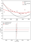 |
Fig. A.1. Top panel: MUSE LSF from Bacon et al. (2017) (thick black line) and in LEWIS data (thick red line, Eq. A.1). The red dashed line represents the MUSE LSF derived restricting the polynomial fit to λ > 5700 Å (Eq. A.2). The thin horizontal black line marks the spectral resolution of the E-MILES stellar library (FWHM = 2.51Å). Bottom panel: comparison of PPXF results for Bacon et al. (2017) LSF (black), LEWIS LSF (red, Eq. A.2) and constant LSF (grey, FWHM[4800-7000] = 2.69Å). |
All Tables
1D and 2D stellar kinematics and dynamical masses of UDGs and LSBs in the Hydra I cluster.
All Figures
|
Fig. 1. Velocity and phase-space distributions of galaxies in Hydra I. Left panel: Distributions of the systemic velocity for galaxies in the LEWIS sample (light blue histogram), bright galaxies (mB < 16 mag, grey histogram) and dwarf galaxies (blue histogram) in Hydra I. The vertical dashed line represents the average cluster velocity (VHydra = 3683 ± 46 km s−1, from Christlein & Zabludoff 2003), and the vertical dotted lines mark the cluster velocity dispersion (σHydra = 724 ± 31 km s−1, from Lima-Dias et al. 2021). Right panel: Phase-space diagnostic diagram for galaxies in Hydra I. The systemic galaxy velocity relative to the average velocity of the cluster normalised by the cluster velocity dispersion (|Vsyst − VHydra|/σHydra) is shown as a function of the projected clustercentric distance normalised by the virial radius of the cluster (R/R200). Galaxies from the LEWIS sample are marked with light blue circles, and galaxies from Christlein & Zabludoff (2003) are marked with white dots. The black diamonds mark the objects with an irregular morphology (UDG8, UDG20, LSB4, and LSB6) described in Section 3. The shaded regions represent the very early (dark grey) and late infall or mixed times (light grey) regions (Rhee et al. 2017; Forbes et al. 2023). |
| In the text | |
|
Fig. 2. Stacked (1D) and spatially resolved (2D) stellar kinematics of UDG1. Top left panel: MUSE-reconstructed image of UDG1. The red ellipse represents the elliptical region we used to extract the stacked spectrum within 1Reff, and the grey circles show the masked image regions. The top label reports the values of the semi-major axis (a), position angle (PA), and ellipticity (ϵ) of the ellipse. Top right panel: MUSE 1Reff stacked spectrum (solid black line) for UDG1. The bottom label reports the fit type (Table 2). The main absorption features are marked with magenta lines and labels. The solid red line represents the best-fitting spectrum obtained with PPXF. The green points show the residuals between the observed and its best-fitting spectrum. The grey areas show the masked spectral regions that we excluded from the fit. The residual points excluded from the fit are marked in blue. Bottom left panel: Voronoi-binned map of the S/N. Bottom middle panel: Stellar velocity map subtracted from the systemic velocity Vsys. The top label reports the type of rotation (Table 2). The blue and red lines mark the photometric major and minor axes of the galaxy, respectively. Bottom right panel: Velocity profiles extracted along the major (top) and minor (bottom) axes and subtracted from Vsys. |
| In the text | |
|
Fig. 3. Distributions of velocity dispersions and rotation curve semi-amplitudes of LEWIS sample. Left panel: Distributions of σeff of UDGs from literature (green histogram) and the LEWIS sample. The light blue histogram corresponds to the distribution of galaxies with a constrained fit (C-fit type). Right panel: Distribution of ΔV of UDGs in the LEWIS sample. The pink and blue histograms correspond to UDGs with a mild rotation along any axis (R and IR type) and those without rotation (NR type), respectively. |
| In the text | |
|
Fig. 4. Faber-Jackson relation and dark matter content in LEWIS sample. Left panel: Velocity dispersion σeff as a function of stellar masses of UDGs from the literature (green diamonds) and the LEWIS sample. The blue and red circles represent rotating and non-rotating LEWIS galaxies, respectively. The shaded light blue region represents the luminosity Faber-Jackson relation, extrapolated to the low-mass regime (L ∼ σ2.2, Kourkchi et al. 2012). The luminosities are converted into stellar masses using the Into & Portinari (2013) colour – M/L relation. UDG7 and UDG12 are marked with triangles since their values of σeff might be overestimated due to their non-negligible rotation. Right panel: Dynamical mass (Mdyn) as a function of the V-band total luminosity (LV, eff) computed within 1Reff of UDGs from the literature (green diamonds) and the LEWIS sample. The points are colour-coded as in the left panel. The solid grey lines mark the loci in the plane where Mdyn/LV, eff is constant and equal to 1, 10, 100, 1000, and 10 000, respectively. The magenta points represent the dwarf galaxies in the Local Group analysed by Battaglia & Nipoti (2022). |
| In the text | |
|
Fig. 5. Kinematic support in LEWIS sample. Projected specific angular momentum (λR) as a function of galaxy ellipticity (left panel) and stellar mass (right panel). The light blue circles mark the LEWIS galaxies, and the pink squares represent the dwarf galaxies studied by Scott et al. (2020). The black curve in the left panel ( |
| In the text | |
|
Fig. 6. Correlations between structural properties and cluster environment. Left panel: Stellar mass as a function of the cluster-centric distance. Middle panel: σeff as a function of the cluster-centric distance. Right panel: Dynamical mass-to-light ratio Mdyn/LV, eff as a function of the cluster-centric distance. The vertical dashed grey line marks the radial distance within which the X-ray emission of the cD galaxy dominates (14 arcmin, Spavone et al. 2024). The labels identify the LEWIS galaxies. Filled circles represent galaxies classified as very early infall, and empty circles represent galaxies classified as late infall or mixed times. The blue and red circles represent rotating and non-rotating galaxies, respectively. The yellow line represents a linear fit obtained by excluding the values for UDG7 and UDG12. The uncertainties on the fitting lines were computed using a bootstrap technique. In the central and right panels, UDG7 and UDG12 are marked with triangles since their values of σeff and Mdyn/LV, eff might be overestimated due to their non-negligible rotation. |
| In the text | |
|
Fig. 7. Correlations between kinematic properties and cluster environment. Semi-amplitude of the rotation curve ΔV as a function of the cluster-centric distance. The data points are colour-coded according to the values of the Reff (left panel), colour g − r (central panel), and σeff (right panel). As in Figure 6, the vertical dashed line marks the extension of the X-ray emission. The circles represent galaxies that rotate along the photometric major axis or intermediate axis (R and IR-type), and triangles show galaxies without rotation (NR-type). |
| In the text | |
|
Fig. A.1. Top panel: MUSE LSF from Bacon et al. (2017) (thick black line) and in LEWIS data (thick red line, Eq. A.1). The red dashed line represents the MUSE LSF derived restricting the polynomial fit to λ > 5700 Å (Eq. A.2). The thin horizontal black line marks the spectral resolution of the E-MILES stellar library (FWHM = 2.51Å). Bottom panel: comparison of PPXF results for Bacon et al. (2017) LSF (black), LEWIS LSF (red, Eq. A.2) and constant LSF (grey, FWHM[4800-7000] = 2.69Å). |
| In the text | |
Current usage metrics show cumulative count of Article Views (full-text article views including HTML views, PDF and ePub downloads, according to the available data) and Abstracts Views on Vision4Press platform.
Data correspond to usage on the plateform after 2015. The current usage metrics is available 48-96 hours after online publication and is updated daily on week days.
Initial download of the metrics may take a while.