| Issue |
A&A
Volume 694, February 2025
|
|
|---|---|---|
| Article Number | A150 | |
| Number of page(s) | 11 | |
| Section | Stellar structure and evolution | |
| DOI | https://doi.org/10.1051/0004-6361/202452727 | |
| Published online | 11 February 2025 | |
Frozen and β-equilibrated f and p modes of cold neutron stars: Nuclear metamodel predictions
CNRS/in2p3, Université Normandie, Ensicaen, LPC-Caen, 14050 Caen, France
⋆ Corresponding authors; This email address is being protected from spambots. You need JavaScript enabled to view it.
, This email address is being protected from spambots. You need JavaScript enabled to view it.
, This email address is being protected from spambots. You need JavaScript enabled to view it.
Received:
23
October
2024
Accepted:
22
December
2024
Abstract
Context. When the chemical re-equilibration timescale is sufficiently long, the normal and quasi-normal mode frequencies of neutron stars should be calculated in the idealised limit that the internal composition of each fluid element is fixed over the oscillation period. However, many studies rely on a barotropic equation of state, implicitly overlooking potential out-of-β-equilibrium effects.
Aims. We investigate potential biases that may arise from the assumption of purely barotropic models in studies of oscillation modes. To address this, we calculated the non-radial fundamental (f) and first pressure (p1) modes for a wide range of neutron star structures, each characterised by different nucleonic equations of state. This approach also yields posterior distributions for the oscillation frequencies, which could be detected by next-generation gravitational wave interferometers.
Methods. A wide range of nuclear equations of state are generated with the metamodel technique, a phenomenological framework that incorporates constraints from astrophysical observations, experimental nuclear physics, and chiral effective field theory. The metamodel also provides the internal composition of β-equilibrated npeμ matter, allowing us to calculate oscillation modes beyond those supported by a purely barotropic fluid.
Results. By exploiting the observed validity of quasi-universal relations, we developed a simple technique to estimate the general relativity corrections in relation to the commonly used Cowling approximation and provide a posterior predictive distribution of expected f- and p1-mode frequencies.
Key words: asteroseismology / dense matter / equation of state / gravitational waves / stars: neutron
© The Authors 2025
 Open Access article, published by EDP Sciences, under the terms of the Creative Commons Attribution License (https://creativecommons.org/licenses/by/4.0), which permits unrestricted use, distribution, and reproduction in any medium, provided the original work is properly cited.
This article is published in open access under the Subscribe to Open model. This email address is being protected from spambots. You need JavaScript enabled to view it. to support open access publication.
1. Introduction
Neutron stars (NSs) can sustain a variety of oscillation modes due to their stratified internal structure and composition. These normal (or quasi-normal, when the frequency is complex) oscillation modes include fundamental (f), pressure (p), and gravitational (g) modes, among others, each characterised by distinct frequencies and damping times (Thorne & Campolattaro 1967; Reisenegger & Goldreich 1992; Andersson et al. 1996; Kokkotas & Schmidt 1999). A detection of gravitational waves (GWs) emitted by quasi-normal oscillations would allow the direct observation of the dominant mode frequencies, enabling a new way of probing NSs’ internal properties and dynamical processes (Andersson 2021; Jones 2022; Andersson 2019). For example, it has been suggested that the p1 mode carries information that can be used to distinguish between nucleonic, hybrid, and strange stars (Vásquez Flores & Lugones 2014). To date, forthcoming runs of LIGO, Virgo, Kagra gravitational wave interferometers, and the planned Einstein Telescope and Cosmic Explorer represent a promising avenue for detecting these oscillations (Andersson et al. 2011; Piccinni 2022; Jones 2022). This holds the appealing prospect of integrating such observations with other data – such as results from NICER (Özel et al. 2016) and the planned Athena spacecraft (Majczyna et al. 2020) – to constrain the equation of state of dense matter.
For cold NSs, the subject of this study, non-radial f modes are expected to be excited during magnetar flares (Levin & van Hoven 2011; Ball et al. 2024) and pulsar glitch events (van Eysden & Melatos 2008; Bennett et al. 2010; Ho et al. 2020); we invite the reader to consult (Antonelli et al. 2022; Haskell & Jones 2024) for a recent review and Yim et al. (2024) for an analysis of glitching pulsar candidates as priority targets of future observations. This is an attractive possibility, as future detections of these modes may be used to discriminate between neutron and quark stars (Wilson & Ho 2024; Sotani et al. 2011).
In addition to probing the internal structure of NSs, oscillation modes can be used to disentangle macroscopic characteristics such as mass and radius when used in tandem with other observations. In fact, Andersson & Kokkotas (1998) found a set of quasi-universal (QU) relations – in the sense that they are almost EoS-independent relations (Yagi & Yunes 2017) – between the normal mode frequencies and the average density or the compactness. To date, there are numerous studies presenting different QU relations for mode frequencies, usually tested with a small sample of EoSs (Tsui & Leung 2005; Benhar et al. 2004; Pradhan et al. 2022; Sotani 2021) or a large set of purely barotropic (namely, zero temperature and β-equilibrated) agnostic matter models of the kind used in, for example, Lindblom (2010), Breu & Rezzolla (2016), Fasano et al. (2019), Moustakidis et al. (2017), Yao et al. (2024). We will perform a systematic study of proposed QU relations for nucleonic NSs’ oscillation modes by using a large set of EoS models that are compatible with the latest astrophysical observations and nuclear physics constraints. This is done by using the phenomenological metamodel technique (Margueron et al. 2018), which allows us to explore the parameter space of cold npeμ EoSs and, at the same time, to include the constraints from the chiral effective theory, experimental nuclear physics, and astrophysical observations via a Bayesian framework (Zhang et al. 2018; Carreau et al. 2019a; Güven et al. 2020; Dinh Thi et al. 2021a). Furthermore, the metamodel is able to reproduce existing realistic nucleonic models and interpolate between them (Mondal & Gulminelli 2022; Davis et al. 2024).
A downside of exploring a wide parameter space for the metamodel representation of the EoS is that we have to find the f- and p1-mode frequencies for a large set of stellar structures, making it impractical to calculate the frequencies in full general relativity. Therefore, we chose to work within the Cowling approximation, which greatly speeds up the computation of the frequencies. In doing so, we also tested the impact of assuming two opposite idealised limits1 for matter undergoing time-dependent compression (Haensel et al. 2002; Andersson 2019), which are described below.
-
Frozen regime – In this limit, the local relaxation processes that bring back npeμ matter back to β equilibrium do not have time to occur, as the compression-expansion cycle imparted by the oscillation is faster than the typical reactions mediated by the weak interaction. This limit is characterised by the local conservation of the chemical fractions, meaning that fractions are purely advected by the fluid motion. This is the limit expected to hold in cold NSs.
-
Equilibrium regime – In this limit, the relaxation processes are so fast that each fluid element has a negligible departure from β equilibrium, so the matter model reduces to that of a perfect barotropic fluid. Given that the relaxation processes are mediated by the weak interaction, this limit might be expected to hold only in high temperature processes, such as proto-NSs and post-merger oscillations.
Similar to the approach taken for non-compact stars (Hansen & Kawaler 1994), evaluating the mode frequencies requires knowledge of the adiabatic index, which determines how pressure responds to changes in local baryonic density (Thorne & Campolattaro 1967; Shapiro & Teukolsky 1983). The choice of one of the two limits can significantly impact the local value of the adiabatic index and, consequently, the pressure response of npeμ matter (Haensel et al. 2002; Andersson 2019). In particular, calculating mode frequencies using a barotropic equation of state and a consistent adiabatic index inherently assumes an equilibrium regime.
To investigate the frozen regime, we need an EoS model that is not purely barotropic, allowing the pressure (or adiabatic index) to be calculated at fixed chemical fractions. The metamodel representation of the cold (neutrinoless) npeμ EoS provides this possibility, enabling a systematic comparison of mode frequencies derived from a purely barotropic EoS versus those that account for the effects of a frozen composition.
In this work, we extended the type of Bayesian analysis performed in previous studies (Zhang et al. 2018; Carreau et al. 2019a; Güven et al. 2020; Dinh Thi et al. 2021a; Davis et al. 2024) by solving, for a large set of metamodel instances, the perturbation equations in the Cowling approximation in the two idealised – that is, frozen and equilibrated – regimes, testing possible deviations from the proposed QU relations. In Sect. 2, we recall the relevant properties the metamodel representation of the energy of cold npeμ matter. Sect. 3 outlines the Bayesian technique developed for our inference: a large number of metamodel instances are assigned with a likelihood depending on how they satisfy astrophysical and nuclear constraints. Then, in Sect. 4, we summarise how the mode frequencies are obtained for each metamodel instance. Finally, the resulting mode frequencies and their posterior distributions – which may be interpreted as a possible frequency range for a future detection – are given in Sect. 5.
2. Metamodel representation of the equation of state and internal composition
The metamodel representation of the nucleonic EoS of an NS was introduced in Margueron et al. (2018). The fundamental assumption is that an NS’s core consists of npeμ matter in weak equilibrium, disregarding the possibility of having other degrees of freedom; albeit, it is possible to modify it to account for phase transitions to quark matter (Mondal et al. 2023). The EoS for the uniform npeμ matter in the core is then consistently prolonged to the lower density layers of the solid crust thanks to the compressible liquid-drop model approach described in Carreau et al. (2019b) and Dinh Thi et al. (2021b). Although not as microscopic as other approaches, this method reproduces results that are consistent with extended Thomas-Fermi calculations at both zero (Grams et al. 2022) and finite temperature (Carreau et al. 2020). Furthermore, it enables the quantitative estimation of a unified EoS for both the core and the crust at a relatively low computing cost.
Within the metamodel technique, each unified2 EoS model is represented by ten independent empirical parameters that correspond to the coefficients of a fourth-order Taylor expansion of the uniform matter binding energy in the isoscalar and isovector channels around saturation density. For non-homogeneous matter, they are supplemented by five further surface and curvature parameters (Dinh Thi et al. 2021b), which are selected by fitting the experimental atomic-mass evaluation nuclear-mass table (Huang et al. 2021) for each set of the ten aforementioned parameters. The density dependence of the symmetry energy and the energy in symmetric matter are characterised by these parameters, and over a wide range of nuclear data, their prior distribution is in agreement with current empirical information (Margueron et al. 2018). Three more parameters are needed: two to account for the density dependence of the effective mass and the effective mass splitting; and one that enforces the correct behaviour at zero density, for a total of 13 independent parameters.
As far as this study is concerned, the metamodel can be thought of as a procedure, denoted as ℳ,
 (1)
(1)
which takes the values of 13 nuclear matter parameters X as input and outputs a β-equilibrated equation of state (EoS) and the composition of the entire star, including the crust. In practice, ℳ provides the β-equilibrated total energy density ϵ, pressure P, electron and muon fractions, and nuclear asymmetry δ (i.e. δ = 1 − 2xp, where xp is the proton fraction), all as functions of the baryon number density nB. We refer the reader to Margueron et al. (2018), Mondal & Gulminelli (2022), and Davis et al. (2024) for an extensive presentation of the nuclear metamodel and its astrophysical applications. Here, we only note that we added the equilibrated vβ and frozen vFR sound speeds to the metamodel output, which will be important in Sect. 4. Given non-informative priors on the 13 nuclear matter parameters X, the resulting metamodel realisation3 ℳ(X) undergoes a Bayesian filtering process that assigns a likelihood ℒ(X), which is detailed in the next section.
3. Likelihood of metamodel realisations
The metamodel instances ℳ(X) are not all equally realistic, in the sense that some give rise to, say, an EoS that is inconsistent with astrophysical observations, or they are not able to reproduce some experimental nuclear phenomenology. Therefore, we assigned a likelihood ℒ(X) to each ℳ(X) via a sequence of Bayesian filters, similar to the ones detailed in Dinh Thi et al. (2021a) and Davis et al. (2024). The reader may also consult Scurto et al. (2024), Char et al. (2023) and Malik et al. (2024) for a similar approach with the relativistic mean field. This filters are set out as follows.
-
The nuclear model ℳ(X) must be consistent with the energy per nucleon of pure neutron matter obtained by ab initio calculations employing chiral effective interactions (χ-EFT) and renormalisation group methods. The conflation of results in the literature obtained from different many-body methods results in an energy band (Huth et al. 2021), which is used to build an informed prior.
-
The nuclear model ℳ(X) must reproduce the nuclear mass measurements in the AME2020 mass table (Huang et al. 2021).
-
The β-equilibrated EoS obtained from ℳ(X) must support a maximum TOV mass greater than that of PSR J0348+0432, as measured by Antoniadis et al. (2013). Additionally, β-equilibrated matter must be stable and causal at least up to the central density of the star with the maximum TOV mass.
-
Similarly, we implement the constraint on the tidal deformability from the GW170817 event (Abbott et al. 2019); see Appendix B.
-
Finally, we implement constraints from the mass-radius X-ray pulse-profile estimates of the masses and radii of PSR J0030+0451, PSR J0437−4715, and PSR J0740+6620 (Vinciguerra et al. 2024; Choudhury et al. 2024; Salmi et al. 2024).
Compared to the previous works on this matter, the main difference lies in how we implement the causality constraint, which is part of point iii and is discussed later, and how we handle the information from χ-EFT calculations. In fact, we take care of point i by constructing an χ-EFT-informed prior via a Metropolis-Hastings sampling, as discussed in Sect. 3.1. Then, we randomly extract 105 models ℳ(X) from this informed prior and pass them trough the sequence of Bayesian filters (ii-v), each of which is assigned a partial likelihood ℒi(X). The total likelihood of each metamodel instance ℳ(X) is
 (2)
(2)
where p(Dj|ℳ(X)) is the conditional probability of reproducing the data, Dj, assuming the metamodel instance, M(X), and the index, j, runs over all the aforementioned constraints. Clearly, ℒ(X) is automatically also the likelihood of all the stellar properties (e.g. mass-radius relation; mode frequencies) that can be derived by assuming the matter model ℳ(X).
3.1. Informed prior from the χ-EFT band
Here, we discuss point i above in more detail. State-of-the-art χ-EFT calculations provide the energy per particle e(n)±δe(n) of pure neutron matter, where 0.02 < n < 0.2 fm−3 is the neutron density and δe(n) is the uncertainty associated with the specific calculation. Since different theoretical approaches yield different (overlapping) energy bands, e(n)±δe(n), we combine all the bands presented in Huth et al. (2021) into a single ‘conflated’ band, where the lower limit is given by the unitary gas approach (see Appendix A). This ensures that we do not underestimate the uncertainty associated with the theoretical calculations of e(n). Specifically, our conflated band is interpreted as a 90% confidence interval for e(n): for each n, the band is represented by a continuous probability density p(e|n) that is flat within the conflated band and has Gaussian tails accounting for the remaining 5%+5% (see Eq. (A.2)). This helps achieve a faster burn-in of the Metropolis-Hastings algorithm. Moreover, the Metropolis-Hastings procedure applied to p(e|n) allows us to to directly sample the nuclear parameters X for which eX(n) obtained from ℳ(X) lies within our conflated band. This process starts with a flat prior4 for the nuclear parameters X. The resulting posterior is then used as an informed prior for filters (ii-v). This approach provides approximately 109 nuclear models ℳ(X) in the informed prior, which is the most selective yet the least computationally demanding one.
3.2. Low-density filters from nuclear phenomenology
Each metamodel instance ℳ(X) can be used to calculate the mass MNZ(X) of a nucleus with N neutrons and Z protons. To do so, a compressible liquid drop model is used, supplemented by five extra surface and curvature parameters (Carreau et al. 2019b; Dinh Thi et al. 2021b). Therefore, to implement a filter (iii), we compare MNZ(X) with the measured nuclear masses  listed in the AME2020 mass table (Wang et al. 2021). Following Dinh Thi et al. (2021a), we assign a partial likelihood of zero – that is, M(X) is discarded – if it is impossible to find values for the five curvature and surface parameters that are consistent with nuclear phenomenology. Otherwise, the partial likelihood is the goodness of the fit:
 (3)
(3)
where the cost function χ2 is
 (4)
(4)
Here, σ is a measure of the theoretical error on nuclear masses5, and the label NZ runs over all the NAME nuclei listed in the mass table.
The model distribution after applying filters (i-ii) yields a posterior distribution for the nuclear parameters X that is consistent with nuclear physics information up to the saturation density. At this stage, for every ℳ(X) that has not been excluded, we can extract the unified β-equilibrated EoS and all relevant outputs in Eq. (1) for all layers, including the crust.
3.3. High-density filters from astrophysics
Astrophysical constraints are applied through filters (iii-v), which are more sensitive to how ℳ(X) describes matter above the saturation density. The first check is hard, in the sense that the partial likelihood is either zero or one; the Tolman-Oppenheimer-Volkoff (TOV) equations are solved, and the maximum TOV mass m*(X) is extracted. We assign a unit multiplicative contribution to the total likelihood in Eq. (2) for any model that satisfies causality and thermodynamic stability (i.e. 0 < vβ2 < vFR2 < 1; see Camelio et al. 2023 for formal proof) and has a non-negative symmetry energy in the range of 0 < nB < n*(X), where n*(X) is the central density of the star with mass m*(X). Otherwise, the model’s likelihood ℒ(X) is set to zero (i.e. the instance ℳ(X) is discarded).
After this preliminary hard filter, we can go through the remaining filters (iii-v), which require the mass-radius relation and tidal deformability and are implemented as in Dinh Thi et al. (2021a), Scurto et al. (2024), Char et al. (2023) and Davis et al. (2024). We briefly list them below and refer to previous work for further details.
To implement filter iii, we require the maximum TOV mass m*(X) to exceed the measured mass of PSR J0348+0432, M = 2.01 ± 0.04 M⊙ (Antoniadis et al. 2013). The resulting contribution to the total likelihood is
 (5)
(5)
Filter iv uses data from GW170817 and is based on the comparison between the effective dimensionless tidal deformability  calculated with ℳ(X) and the data of the Ligo-Virgo Collaboration (LVC). The likelihood takes the following form (see Appendix B for details):
 (6)
(6)
where  is the effective tidal deformability, q < 1 is the mass ratio of the lighter object over the heavier one, and
  is the observational joint posterior distribution reported in Abbott et al. (2019).
Finally, in filter v we check if the mass-radius relation RX(m) obtained with the nuclear model ℳ(X) is consistent with the updated NICER estimates of the joint mass-radius distributions for three pulsars:
 (7)
(7)
where P1 is the joint probability distribution of mass and radius of the PSR J0030+0451 pulsar (Vinciguerra et al. 2024), P2 refers to PSR J0437−4715 (Choudhury et al. 2024), and P3 refers to PSR J0740+6620 (Salmi et al. 2024).
4. Frozen and equilibrated normal modes
The Bayesian procedure outlined in the previous section allows us to assign a likelihood to each model ℳ(X) based on its compatibility with nuclear physics phenomenology and astrophysical constraints. We now proceed to compute the normal mode frequencies, with the double aim of checking the impact of chemical transfusion and obtaining a posterior predictive distribution based on ℒ(X) for the mode frequencies.
4.1. Numerical scheme for the normal mode frequencies
First, we recall how to determine the frequencies of the f and p1 normal modes of a spherically symmetric non-rotating NS in the relativistic Cowling approximation (McDermott et al. 1983). Since the space time remains unperturbed, no gravitational waves are emitted and, consequently, the radiation damping is absent. Moreover, the two equilibrated and frozen limits we considered are non-dissipative regimes (e.g. Gavassino et al. 2021, Sect. II-D), implying that there is no bulk viscosity damping due to reactions (e.g. Sawyer 1989; Haensel et al. 2002; Schmitt & Shternin 2018; Alford & Harris 2019; Alford et al. 2023). This limits our study to purely real frequencies.
Following Sotani et al. (2011), and consistently with the more complete full-GR derivation in Lindblom & Detweiler (1983), Sotani et al. (2001), the spherical space-time metric is
 (8)
(8)
while the Lagrangian fluid displacement (see Thorne & Campolattaro 1967) is a three-vector ξi(t, r, θ, ϕ) defined with respect to the space-like part of the coordinate basis:
 (9)
(9)
where  and
and  characterise the amplitude of the perturbation and Ylm are the spherical harmonics, as in Lindblom & Detweiler (1983) and Sotani et al. (2001). Using these variables, the equations for the oscillation modes are
![Mathematical equation: $$ \begin{aligned} \frac{\mathrm{d}W}{\mathrm{d}r}&= \left(\frac{\mathrm{d}P}{\mathrm{d}\epsilon } \right)^{-1} \left[\omega ^2r^2e^{\Lambda -2\Phi }V+\frac{\mathrm{d}\Phi }{\mathrm{d}r}W\right] - l(l+1)e^{\Lambda }V \nonumber \\ \frac{\mathrm{d}V}{\mathrm{d}r}&= 2\frac{\mathrm{d}\Phi }{\mathrm{d}r}V - \frac{1}{r^2}e^\Lambda W, \end{aligned} $$](/articles/aa/full_html/2025/02/aa52727-24/aa52727-24-eq16.gif) (10)
(10)
where we take l = 2, since we focus on quadrupolar oscillations. The different regime of the balance between oscillation frequency and reaction rate is determined by the term dP/dϵ, the squared speed of sound, which encodes information equivalent to that in the adiabatic index (e.g. Haensel et al. 2002; Andersson 2019).
Boundary conditions at the star centre and surface are required to solve the system in Eq. (10). An inspection of the system shows that W(r) = Crl + 1 + 𝒪(rl + 3) and V(r) = Crl + 𝒪(rl + 2) for r → 0, with C being an arbitrary constant. The other boundary condition is obtained by demanding that the pressure perturbation vanishes at the stellar surface, which leads to
 (11)
(11)
With this condition, the problem becomes an eigenvalue one, which we solve using a standard shooting method. After determining the metric functions and stellar structure by solving the TOV equations, we solve the system in Eq. (10) using an initial guess for the (purely real and positive) pulsation ω. We then refine the value of ω with a bisection method, iterating the process until we find the exact ω that satisfies Eq. (11).
4.2. Frozen speed of sound and the thermodynamic stability-causality condition
For perturbations that are slow enough, matter will be always almost in β equilibrium, and dP/dϵ in Eq. (10) can be taken to be vβ2, the sound speed arising from a purely barotropic EoS:
 (12)
(12)
On the other hand, in a fast oscillation regime the composition of each fluid element has no time to relax and return to chemical equilibrium, and one should use the sound speed vFR2 at frozen composition, which we conveniently write as
 (13)
(13)
As discussed in Camelio et al. (2023), the velocity vFR coincides with the ‘maximal characteristic speed’ (the speed defining the Courant-Friedrichs-Lewy condition) for a signal propagating in a chemically reacting fluid mixture, implying that the mixture is both thermodynamically stable and causal6 only if
 (14)
(14)
From the point of view of global oscillations, particularly in g modes (e.g. Lai 1994; Jaikumar et al. 2021; Tran et al. 2023), the same criterion guarantees the local convective stability of the star (see Eq. (A.12) of Camelio et al. 2023 with Eq. (4.17) in Lai 1994). Therefore, as mentioned in Sect. 3.3, we only retain the metamodel instances ℳ(X) that satisfy the fundamental thermodynamic stability-causality condition 0 < vβ2(nB) < vFR2(nB) < 1 at least up to the central density of the NS with maximum TOV mass.
5. Results and discussion
For each nuclear model, ℳ(X), we extracted the f and p1 normal mode frequencies in the Cowling approximation, with the purpose of testing the QU relations with a large set of metamodel instances and quantifying the potential impact of assuming frozen or equilibrated composition. Finally, we used the known QU relation in full GR to estimate a more realistic posterior predictive distribution for the mode frequencies.
5.1. Differences between frozen and barotropic frequencies
We evaluated the Cowling frequencies of the f and p1 modes in the two ideal limits of frozen and equilibrated composition, as outlined in the previous section. The results in the β-equilibrated case are shown in Fig. 1, where the prediction of the model associated with the highest likelihood are given by solid lines. We can see that, though the two modes are clearly separated, accounting for the uncertainty in the nucleonic model leads to an important dispersion of the predictions, particularly for the p1 case. As a consequence, the discrimination between hadronic and strange stars from the measured value of the p1 frequency might be harder than expected in first works that only considered a limited set of hadronic models (e.g. Vásquez Flores & Lugones 2014).
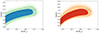 |
Fig. 1. Probability density distributions for f-mode frequencies (left) and p1-mode frequencies (right), both obtained within the Cowling approximation in the barotropic limit. The three shaded regions refer to the 68%, 95%, and 99% percentiles. The solid black line represents the model with the highest likelihood. |
The frequencies of the f mode are almost unaffected by the equilibration assumption, with differences smaller than 0.5%, as shown in Fig. 2. On the other hand, the p1 mode exhibits a more interesting behaviour, where the differences between the two cases are more evident and tend to increase with mass, as can be seen in Fig. 3. However, for the models with high likelihood, the ones in the darkest region of the plot, the frequencies calculated in the frozen limit remain close to the ones obtained by assuming the barotropic sound speed.
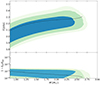 |
Fig. 2. Posterior probability density for frequencies of frozen f-mode (upper panel). The lower panel shows the relative difference between the frequencies in the frozen limit and the barotropic limit. The shaded regions represent the 68%, 95%, and 99% percentiles, respectively, while the black line indicates the model with the highest likelihood. |
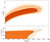 |
Fig. 3. Posterior probability density for frequencies of frozen p1 mode (upper panel). The lower panel shows the relative difference between the frequencies in the frozen limit and the barotropic limit. The three shaded regions correspond to the 68%, 95%, and 99% percentiles, while the black line represents the model with the highest likelihood. |
Based on these results, only the frozen frequencies are presented in the subsequent discussion, as the differences are negligible for the f mode and less than 5% for the p1 mode in reasonable mass ranges (not too close to the maximum TOV mass). For the same reason, the present analysis confirms – on the basis of a large set of nuclear models – that when the frozen speed of sound or the frozen adiabatic index is unavailable, the β-equilibrated speed of sound vβ can be used with minimal error. Namely, f and p1 modes obtained with agnostic barotropic models can be trusted within 5% or better, especially for masses below ∼2 M⊙.
5.2. Test of proposed quasi-universal relations
Andersson & Kokkotas (1998) proposed a QU relation for the for the p1 mode, where the mode pulsation ω times the NS mass M was expressed in terms of the compactness M/R. This same scaling was later used to look for a QU relation for the f mode by Tsui & Leung (2005):
 (15)
(15)
where the coefficients ai are obtained from a fit over a limited number of barotropic EoS models. This empirical expression was recently tested with a2 = a3 = 0 for the f mode in the Cowling approximation (Pradhan & Chatterjee 2021) and with a3 = 0 for the f mode in full GR (Pradhan et al. 2022). Moreover, Sotani (2021) applied the empirical relation (15), including all coefficients, to the p1-mode frequencies in full GR (see Table 1).
As a preliminary check, we evaluated the accuracy of the QU relation (15) using our set of metamodel instances in order to assess the quality of the proposed fits and the dispersion of the metamodel instances around them. The results are presented in Fig. 4, where we compare our findings with the fits from the aforementioned works (the coefficients of these fits are listed in Table 1, along with a fit of the p1 mode to our numerical results). The first panel of Fig. 4 shows the density map of mode frequencies resulting from our Bayesian filtering, with the f mode in blue-green and the p1 mode in orange-yellow, alongside the various QU relations mentioned earlier.
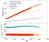 |
Fig. 4. Relationship between rescaled pulsations ωM and compactness M/R for the frozen f modes (blue-green) and frozen p1 modes (orange-yellow). The dashed lines correspond to the fits presented in Table 1, while the solid black line represents the model ℳ(X) with the highest likelihood ℒ(X). The fit lines overlapping with the distributions are based on the Cowling approximation, whereas the others, obtained in full GR, are shown for comparison. The differences between the rescaled pulsations ωM calculated in the Cowling approximation and the corresponding QU fits are illustrated in the two lower panels. Each panel also includes three shaded regions representing the 68%, 95%, and 99% quantiles of the distribution. |
To quantify the dispersion of the metamodel instances around the QU fits, the two lower panels of Fig. 4 display the differences between our numerical results and the Cowling QU fitting formula. In both lower panels of Fig. 4, the dispersion around the proposed f-mode QU fit is minimal, demonstrating that our extensive set of EoSs adheres to it with the expected level of precision, with errors smaller than 2.5%. However, a structure in the residuals remains visible, which can be attributed to the choice of a linear fit. In contrast, the functional form for the fit of the p1-mode QU seems appropriate, as there are no evident underlying structures observed in the dispersion of the residuals. Nevertheless, it is noteworthy that in this case the precision to which the QU relation is realised is lower, with errors ranging from approximately 5% to 10%.
For completeness, we also tested an alternative empirical relation, linking the f-mode frequency and the average density of the star (Andersson & Kokkotas 1998; Pradhan et al. 2022):
 (16)
(16)
where  ,
,  km and the constants a and b are obtained from a fit to the numerical results. This relation has been tested by different authors with different barotropic EoSs (not all compatible with the constraint imposed by the measured mass of PSR J0348+0432). Therefore, we verify whether Eq. (16) is a QU relation by using our filtered set of nuclear models. This is shown in Fig. 5, where the upper distribution represents our Cowling results, which is compared to the one obtained by reversing relation Eq. (15) with the coefficients provided in Pradhan et al. (2022). We also compare these distributions to the empirical relations presented in Pradhan et al. (2022), Benhar et al. (2004), and Andersson & Kokkotas (1998). Since these empirical relations are all derived from fits to frequencies extracted in full GR, they are obviously not compatible with our Cowling results. In contrast, the Cowling relation presented in Pradhan & Chatterjee (2021), obtained within the Cowling approximation, is closer to our results. It can be observed that this relation strongly depends on the selected set of EoSs, resulting in a significant spread around the relation in Eq. (16).
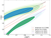 |
Fig. 5. Distributions of f-mode frequencies as a function of the average density |

5.3. Estimation of full-GR mode frequencies
Because of the excellent agreement between Eq. (15) and the metamodel result in the Cowling approximation, we can assume that the dispersion observed in Fig. 4, due to the different softness levels of the nuclear models, will equally affect the degree of validity of the QU relations in full GR. Under this assumption, the QU relation in Eq. (15) can be used to quickly estimate the frequencies for ℳ(X) in full GR directly from the RX(M) relation, as long as the opportune parameters ai are used. We denote these frequencies as ‘synthetic’ since they are not obtained by solving the eigenvalue problem but rather by simply unpacking the QU relation Eq. (15) via the mass-radius relation RX(M) of each ℳ(X).
More precisely, the procedure used to recover the synthetic frequencies fGR in full GR (i.e. beyond the Cowling approximation) is
 (17)
(17)
with Δ given by
 (18)
(18)
where ωC is the mode pulsation that we found within the Cowling approximation in the frozen limit; UC, GR is the Cowling (C) or full-GR (GR) quasi-universal relation, namely the right hand side of Eq. (15) with the appropriate coefficients ai listed in Table 1.
The prescription Eq. (17) for the synthetic frequencies fGR is designed so that we do not underestimate the spread of the p1 frequencies, as discussed in Appendix C. Essentially, we unpack the QU relation in Eq. (15), with the coefficients ai extracted from numerical results in full GR, and transporting the spread of our Cowling calculation onto the unpacked results.
Figure 6 shows the estimated probability density of the synthetic frequencies for the f mode and p1 mode, together with the prediction of the model associated with the highest likelihood. As expected, the f-mode frequency increases more rapidly with mass than the p1-mode one, which remains relatively flat. Consequently, extrapolating NS features from the p1-mode frequencies is expected to be much more challenging. To quantify this further, in Fig. 7 we show the posterior distributions of frequencies for an NS with masses of M = 1 M⊙, 1.4 M⊙, 2 M⊙ in the frozen limit. The three distributions for the p1 mode are nearly indistinguishable, as they almost completely overlap. In contrast, the three distributions for the f mode show only partial overlap, suggesting that it may be possible to constrain the mass of an NS, despite uncertainties in the nuclear EoS. On the other side, the quasi-universality of the p1 frequency in the purely hadronic hypothesis opens the compelling possibility of it being challenged in hybrid or strange stars, as proposed in Vásquez Flores & Lugones (2014) and Wilson & Ho (2024).
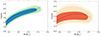 |
Fig. 6. Probability distributions of synthetic full-GR frequencies obtained from Eq. (17). The left panel shows the f mode, while the right one shows the p1 mode. The three shaded regions in each panel contain the 68%, 95%, and 99% percentiles. The solid black line represents the model with the highest likelihood. |
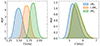 |
Fig. 7. Distribution of synthetic full-GR frequencies at 1 M⊙, 1.4 M⊙, and 2 M⊙ obtained from Eq. (17). The left panel refers to the f mode, while the right one refers to the p1 mode. |
6. Conclusions
With the advent of next-generation interferometers, it becomes important to evaluate how future GW detection from oscillating NSs could be used to constrain nuclear models of neutron star interiors or infer the mass of the object. To address this, we adopted the nuclear metamodel framework (Margueron et al. 2018) for cold npeμ matter, generating a large set of unified equations of state, together with their β-equilibrated composition and the two (barotropic and frozen) sound speeds. These nuclear models were then assigned likelihoods ℒ(X) through a sequence of Bayesian filters, designed to weigh each metamodel instance based on its consistency with established nuclear and astrophysical phenomenology. Given this posterior for the EoSs, we find the posterior predictive distributions for the f- and p1-mode frequencies – shown in Fig. 7 – by inverting known full-GR quasi-universal relations. More precisely, Fig. 7 is our ‘synthetic’ full-GR prediction of the f- and p1-mode frequencies as a function of the NS’s mass: while an f-mode detection could constrain the NS mass, this information is almost completely lost for the p1 mode.
The generation of a large set of metamodel instances and the relative stellar structures for different masses also allowed us to check another point, which is more related to the physical assumptions underlying the computation of the modes. Proposed QU relations pertaining to mode frequencies have been found using barotropic models or, equivalently, non-barotropic nuclear models that are always at strict β equilibrium, namely using dP/dϵ = vβ2 in Eq. (10). Hence, we checked the impact of the more realistic (Haensel et al. 2002) frozen limit assumption, dP/dϵ = vFR2, to see if it could introduce any deviation from the known QU relations for the f and p1 modes. This check is a first, albeit partial, step towards a more systematic study of the impact of nuclear reactions on NS oscillation spectra (see e.g. Counsell et al. 2024a); in principle, reactions introduce mode damping, whose strength depends on the details of the nuclear model and physical conditions of temperature and density (e.g. Haensel et al. 2002; Schmitt & Shternin 2018; Alford & Harris 2019; Alford et al. 2023, 2024). However, in the two ideal limits considered here, any possible bulk-viscous effect is exactly zero (Gavassino et al. 2021; Camelio et al. 2023). This is a caveat to be kept in mind.
Our analysis shows that both the f and p1 modes do not significantly depend on whether the sound speed used is the barotropic or frozen one. This is in contrast with what is known for g modes, where both velocities have to be used to find the frequency spectrum (e.g. Reisenegger & Goldreich 1992; Tran et al. 2023; Zhao & Lattimer 2022; Counsell et al. 2024b). Therefore, we conclude that studies assuming purely barotropic agnostic models for the EoS are accurate to within a few percent. This behaviour is reflected in the goodness of the QU relation, which can thus be used to estimate the mode frequencies without solving the perturbation equations – a crucial advantage in Bayesian studies that involve millions of agnostic EoSs.
Finally, the posterior set of metamodel EoSs obtained through the filtering procedure represents a refinement over previous similar studies (Dinh Thi et al. 2021a; Davis et al. 2024), owing to the implementation of the more stringent stability-causality condition 0 < vβ2 < vFR2 < 1 derived in Camelio et al. (2023). This improved posterior set may also serve as a useful input for further studies on potential constraints on NS interiors, such as those derived from pulsar glitches (Antonelli et al. 2022).
Both limits are non-dissipative: there is no entropy generation due to reaction-mediated bulk viscosity; see e.g. Camelio et al. (2023) or the general discussion in Gavassino et al. (2021, Sect. II-D).
The crust and the core parts of the EoS are built from the same nuclear model ℳ(X) and are matched at a consistent transition density.
The ranges over which each nuclear parameter can vary are wide enough to be fully consistent with up-to-date nuclear phenomenology (Margueron et al. 2018).
The experimental uncertainty in  is always negligible compared to the typical precision with which a compressible liquid drop model approach can reproduce nuclear masses, which is approximately 2 MeV/c2 (Carreau et al. 2019b). Consequently, we set σ = 0.04 MeV/c2, which is consistent with the requirement that
  (Dinh Thi et al. 2021a; Davis et al. 2024).
Namely, the full thermodynamic equilibrium state is stable against fluctuations, and matter perturbations remain within their light-cone envelope (Olson & Hiscock 1989; Gavassino et al. 2022).
Acknowledgments
We thank Hoa Dinh Thi, Micaela Oertel, Chiranjib Mondal and Debarati Chatterjee for useful discussion, and Philip John Davis for technical support. Partial support comes from the IN2P3 Master Project NewMAC, the ANR project “Gravitational waves from hot neutron stars and properties of ultra-dense matter” (GW-HNS, ANR-22-CE31-0001-01), and the CNRS International Research Project (IRP) “Origine des éléments lourds dans l’univers: Astres Compacts et Nucléosynthèse” (ACNu).
References
- Abbott, B. P., Abbott, R., Abbott, T. D., et al. 2019, Phys. Rev. X, 9, 011001 [Google Scholar]
- Alford, M. G., & Harris, S. P. 2019, Phys. Rev. C, 100, 035803 [NASA ADS] [CrossRef] [Google Scholar]
- Alford, M., Harutyunyan, A., & Sedrakian, A. 2023, Phys. Rev. D, 108, 083019 [CrossRef] [Google Scholar]
- Alford, M. G., Haber, A., & Zhang, Z. 2024, Phys. Rev. C, 109, 055803 [NASA ADS] [CrossRef] [Google Scholar]
- Andersson, N. 2019, Gravitational-Wave Astronomy (Oxford: Oxford University Press) [CrossRef] [Google Scholar]
- Andersson, N. 2021, Universe, 7, 97 [NASA ADS] [CrossRef] [Google Scholar]
- Andersson, N., & Kokkotas, K. D. 1998, MNRAS, 299, 1059 [NASA ADS] [CrossRef] [Google Scholar]
- Andersson, N., Kojima, Y., & Kokkotas, K. D. 1996, ApJ, 462, 855 [NASA ADS] [CrossRef] [Google Scholar]
- Andersson, N., Ferrari, V., Jones, D. I., et al. 2011, Gen. Relat. Grav., 43, 409 [CrossRef] [Google Scholar]
- Antonelli, M., Montoli, A., & Pizzochero, P. 2022, Insights Into the Physics of Neutron Star Interiors from Pulsar Glitches (World Scientific), 219 [Google Scholar]
- Antoniadis, J., Freire, P. C. C., Wex, N., et al. 2013, Science, 340, 448 [Google Scholar]
- Ball, M., Frey, R., & Merfeld, K. 2024, MNRAS, 533, 3090 [CrossRef] [Google Scholar]
- Benhar, O., Ferrari, V., & Gualtieri, L. 2004, Phys. Rev. D, 70, 124015 [NASA ADS] [CrossRef] [Google Scholar]
- Bennett, M. F., van Eysden, C. A., & Melatos, A. 2010, MNRAS, 409, 1705 [NASA ADS] [CrossRef] [Google Scholar]
- Breu, C., & Rezzolla, L. 2016, MNRAS, 459, 646 [NASA ADS] [CrossRef] [Google Scholar]
- Camelio, G., Gavassino, L., Antonelli, M., Bernuzzi, S., & Haskell, B. 2023, Phys. Rev. D, 107, 103031 [CrossRef] [Google Scholar]
- Carreau, T., Gulminelli, F., & Margueron, J. 2019a, Phys. Rev. C, 100, 055803 [NASA ADS] [CrossRef] [Google Scholar]
- Carreau, T., Gulminelli, F., & Margueron, J. 2019b, Eur. Phys. J. A, 55, 188 [CrossRef] [Google Scholar]
- Carreau, T., Gulminelli, F., Chamel, N., Fantina, A. F., & Pearson, J. M. 2020, A&A, 635, A84 [NASA ADS] [CrossRef] [EDP Sciences] [Google Scholar]
- Char, P., Mondal, C., Gulminelli, F., & Oertel, M. 2023, Phys. Rev. D, 108, 103045 [CrossRef] [Google Scholar]
- Choudhury, D., Salmi, T., Vinciguerra, S., et al. 2024, ApJ, 971, L20 [NASA ADS] [CrossRef] [Google Scholar]
- Counsell, A. R., Gittins, F., & Andersson, N. 2024a, MNRAS, 531, 1721 [CrossRef] [Google Scholar]
- Counsell, R., Gittins, F., Andersson, N., & Pnigouras, P. 2024b, ArXiv e-prints [arXiv:2409.20178] [Google Scholar]
- Davis, P. J., Dinh Thi, H., Fantina, A. F., et al. 2024, A&A, 687, A44 [NASA ADS] [CrossRef] [EDP Sciences] [Google Scholar]
- Dinh Thi, H., Mondal, C., & Gulminelli, F. 2021a, Universe, 7, 373 [NASA ADS] [CrossRef] [Google Scholar]
- Dinh Thi, H., Carreau, T., Fantina, A. F., & Gulminelli, F. 2021b, A&A, 654, A114 [CrossRef] [EDP Sciences] [Google Scholar]
- Fasano, M., Abdelsalhin, T., Maselli, A., & Ferrari, V. 2019, Phys. Rev. Lett., 123, 141101 [NASA ADS] [CrossRef] [Google Scholar]
- Gavassino, L., Antonelli, M., & Haskell, B. 2021, Class. Quant. Grav., 38, 075001 [Google Scholar]
- Gavassino, L., Antonelli, M., & Haskell, B. 2022, Phys. Rev. Lett., 128, 010606 [CrossRef] [PubMed] [Google Scholar]
- Grams, G., Somasundaram, R., Margueron, J., & Reddy, S. 2022, Phys. Rev. C, 105, 035806 [CrossRef] [Google Scholar]
- Güven, H., Bozkurt, K., Khan, E., & Margueron, J. 2020, Phys. Rev. C, 102, 015805 [CrossRef] [Google Scholar]
- Haensel, P., Levenfish, K. P., & Yakovlev, D. G. 2002, A&A, 394, 213 [NASA ADS] [CrossRef] [EDP Sciences] [Google Scholar]
- Hansen, C. J., & Kawaler, S. D. 1994, Stellar Interiors. Physical Principles, Structure, and Evolution (New York: Springer) [Google Scholar]
- Haskell, B., & Jones, D. I. 2024, Astropart. Phys., 157, 102921 [NASA ADS] [CrossRef] [Google Scholar]
- Ho, W. C. G., Jones, D. I., Andersson, N., & Espinoza, C. M. 2020, Phys. Rev. D, 101, 103009 [CrossRef] [Google Scholar]
- Huang, W. J., Wang, M., Kondev, F. G., Audi, G., & Naimi, S. 2021, Chin. Phys. C, 45, 030002 [NASA ADS] [CrossRef] [Google Scholar]
- Huth, S., Wellenhofer, C., & Schwenk, A. 2021, Phys. Rev. C, 103, 025803 [CrossRef] [Google Scholar]
- Jaikumar, P., Semposki, A., Prakash, M., & Constantinou, C. 2021, Phys. Rev. D, 103, 123009 [NASA ADS] [CrossRef] [Google Scholar]
- Jones, D. I. 2022, in Astrophysics in the XXI Century with Compact Stars, ed. C. A. Z. Vasconcellos (Singapore: World Scientific), 201 [CrossRef] [Google Scholar]
- Kokkotas, K. D., & Schmidt, B. G. 1999, Liv. Rev. Relat., 2, 2 [NASA ADS] [CrossRef] [Google Scholar]
- Lai, D. 1994, MNRAS, 270, 611 [NASA ADS] [CrossRef] [Google Scholar]
- Levin, Y., & van Hoven, M. 2011, MNRAS, 418, 659 [NASA ADS] [CrossRef] [Google Scholar]
- Lindblom, L. 2010, Phys. Rev. D, 82, 103011 [CrossRef] [Google Scholar]
- Lindblom, L., & Detweiler, S. L. 1983, ApJS, 53, 73 [NASA ADS] [CrossRef] [Google Scholar]
- Majczyna, A., Madej, J., Należyty, M., Różańska, A., & Bełdycki, B. 2020, ApJ, 888, 123 [NASA ADS] [CrossRef] [Google Scholar]
- Malik, T., Dexheimer, V., & Providência, C. 2024, Phys. Rev. D, 110, 043042 [NASA ADS] [CrossRef] [Google Scholar]
- Margueron, J., Hoffmann Casali, R., & Gulminelli, F. 2018, Phys. Rev. C, 97, 025805 [NASA ADS] [CrossRef] [Google Scholar]
- McDermott, P. N., van Horn, H. M., & Scholl, J. F. 1983, ApJ, 268, 837 [Google Scholar]
- Mondal, C., & Gulminelli, F. 2022, Phys. Rev. D, 105, 083016 [NASA ADS] [CrossRef] [Google Scholar]
- Mondal, C., Antonelli, M., Gulminelli, F., et al. 2023, MNRAS, 524, 3464 [CrossRef] [Google Scholar]
- Moustakidis, C. C., Gaitanos, T., Margaritis, C., & Lalazissis, G. A. 2017, Phys. Rev. C, 95, 045801 [NASA ADS] [CrossRef] [Google Scholar]
- Olson, T. S., & Hiscock, W. A. 1989, Phys. Rev. C, 39, 1818 [CrossRef] [Google Scholar]
- Özel, F., Psaltis, D., Arzoumanian, Z., Morsink, S., & Bauböck, M. 2016, ApJ, 832, 92 [CrossRef] [Google Scholar]
- Piccinni, O. J. 2022, Galaxies, 10, 72 [NASA ADS] [CrossRef] [Google Scholar]
- Pradhan, B. K., & Chatterjee, D. 2021, Phys. Rev. C, 103, 035810 [NASA ADS] [CrossRef] [Google Scholar]
- Pradhan, B. K., Chatterjee, D., Lanoye, M., & Jaikumar, P. 2022, Phys. Rev. C, 106, 015805 [NASA ADS] [CrossRef] [Google Scholar]
- Reisenegger, A., & Goldreich, P. 1992, ApJ, 395, 240 [Google Scholar]
- Salmi, T. H. J., Choudhury, D., Kini, Y., et al. 2024, ApJ, 974, 294 [NASA ADS] [CrossRef] [Google Scholar]
- Sawyer, R. F. 1989, Phys. Rev. D, 39, 3804 [NASA ADS] [CrossRef] [Google Scholar]
- Schmitt, A., & Shternin, P. 2018, Astrophys. Space Sci. Lib., 457, 455 [NASA ADS] [CrossRef] [Google Scholar]
- Scurto, L., Pais, H., & Gulminelli, F. 2024, Phys. Rev. D, 109, 103015 [NASA ADS] [CrossRef] [Google Scholar]
- Shapiro, S. L., & Teukolsky, S. A. 1983, Black Holes, White Dwarfs and Neutron Stars. The Physics of Compact Objects (New York: Wiley-Interscience) [CrossRef] [Google Scholar]
- Shen, H., Toki, H., Oyamatsu, K., & Sumiyoshi, K. 1998, Nucl. Phys. A, 637, 435 [Google Scholar]
- Sotani, H. 2021, Phys. Rev. D, 103, 123015 [NASA ADS] [CrossRef] [Google Scholar]
- Sotani, H., Tominaga, K., & Maeda, K.-I. 2001, Phys. Rev. D, 65, 024010 [NASA ADS] [CrossRef] [Google Scholar]
- Sotani, H., Yasutake, N., Maruyama, T., & Tatsumi, T. 2011, Phys. Rev. D, 83, 024014 [NASA ADS] [CrossRef] [Google Scholar]
- Thorne, K. S., & Campolattaro, A. 1967, ApJ, 149, 591 [NASA ADS] [CrossRef] [Google Scholar]
- Tran, V., Ghosh, S., Lozano, N., Chatterjee, D., & Jaikumar, P. 2023, Phys. Rev. C, 108, 015803 [NASA ADS] [CrossRef] [Google Scholar]
- Tsui, L. K., & Leung, P. T. 2005, MNRAS, 357, 1029 [NASA ADS] [CrossRef] [Google Scholar]
- van Eysden, C. A., & Melatos, A. 2008, Class. Quant. Grav., 25, 225020 [NASA ADS] [CrossRef] [Google Scholar]
- Vásquez Flores, C., & Lugones, G. 2014, Class. Quant. Grav., 31, 155002 [Google Scholar]
- Vinciguerra, S., Salmi, T., Watts, A. L., et al. 2024, ApJ, 961, 62 [NASA ADS] [CrossRef] [Google Scholar]
- Wang, M., Huang, W., Kondev, F., Audi, G., & Naimi, S. 2021, Chin. Phys. C, 45, 030003 [CrossRef] [Google Scholar]
- Wilson, O. H., & Ho, W. C. G. 2024, Phys. Rev. D, 109, 083006 [CrossRef] [Google Scholar]
- Yagi, K., & Yunes, N. 2017, Phys. Rep., 681, 1 [NASA ADS] [CrossRef] [Google Scholar]
- Yao, N., Sorensen, A., Dexheimer, V., & Noronha-Hostler, J. 2024, Phys. Rev. C, 109, 065803 [CrossRef] [Google Scholar]
- Yim, G., Shao, L., & Xu, R. 2024, MNRAS, 532, 3893 [NASA ADS] [CrossRef] [Google Scholar]
- Zhang, N.-B., Li, B.-A., & Xu, J. 2018, ApJ, 859, 90 [CrossRef] [Google Scholar]
- Zhao, T., & Lattimer, J. M. 2022, Phys. Rev. D, 106, 123002 [NASA ADS] [CrossRef] [Google Scholar]
Appendix A: The chiral band of neutron matter
The χ-EFT ab-initio calculations taken into account in this work are presented in Fig. 1 of Huth et al. (2021): the i-th approach provides an estimate of ei(n)±δei(n), the energy per baryon of pure neutron matter in the range 0.02 < n < 0.2fm−3 where all approaches are expected to provide reliable results. For each metamodel instance ℳ(X), we can easily extract eX(n), and compare it with the theoretical microscopic results ei(n)±δei(n). To this end, we have to conflate all the bands ei(n)±δei(n) reported in Huth et al. (2021) into a single one, e(n)±δe(n): the lower limit e−(n) = e(n)−δe(n) is given by the unitary gas model, while the upper bound e+(n) = e(n)−δe(n) is
 (A.1)
(A.1)
In order not to underestimate the theoretical systematic error, we interpret [e−(n),e+(n)] as the 90% confidence interval where eX(n) should lie arising from a smooth probability distribution to be used within the metropolis-Hastings algorithm. Namely, we consider the following normalized distribution:
![Mathematical equation: $$ \begin{aligned} p(e|n) = Q_n {\left\{ \begin{array}{ll} \exp \left(-\frac{ (e - e_-(n))^2}{2\sigma _n^2}\right)&\mathrm{if}\; e \in (-\infty ,e_-(n)] \\ 1&\mathrm{if}\; e \in (e_-(n),e_+(n)] \\ \exp \left(-\frac{(e - e_+(n))^2}{2\sigma _n^2} \right)&\mathrm{if}\; e \in (e_+(n),\infty ) \end{array}\right.} \end{aligned} $$](/articles/aa/full_html/2025/02/aa52727-24/aa52727-24-eq31.gif) (A.2)
(A.2)
where
 (A.3)
(A.3)
In this way, the central plateau of the distribution accounts for the 90% while each tail for the remaining 10%, in accordance with other prescriptions used previous studies (Dinh Thi et al. 2021a; Carreau et al. 2019b; Scurto et al. 2024). Then, the partial likelihood of ℳ(X) is given by the geometric product integral
 (A.4)
(A.4)
over the 0.02 < n < 0.2 fm−3 density range. In practice, the density range is divided in N equally spaced slices at densities nj and the resulting likelihood is
 (A.5)
(A.5)
Appendix B: Scheme for the LVC constraint
For completeness, we provide a schematic presentation of the LVC constraint in Eq. (6). This may help the reader sort the details and complement the sketch given in previous works that adopt the same prescription (Dinh Thi et al. 2021a; Mondal & Gulminelli 2022; Scurto et al. 2024; Char et al. 2023; Davis et al. 2024).
The analysis in Abbott et al. (2019) provides the observational joint posterior  for the effective tidal deformability
  and the mass ratio q of GW170817. In principle, both quantities can be determined from the masses mk and tidal deformabilities Λk of the two NSs (k = 1, 2) using known analytical expressions,
  and q(mk). The GW170817 data enabled a relatively precise determination of the chirp mass mc (treated as a given constant in the following), which can also be expressed analytically in terms of the two masses, mc(mk).
To implement the constraint imposed by knowledge of  and mc, the first step is to recognize that we are adopting a framework where the mass M is treated as an independent variable, and ℳ(X) can be used to obtain the relations RX(M) and ΛX(M). This is a natural and convenient choice, considering that RX(M) and ΛX(M) are genuine functions, whereas MX(R) or ΛX(R) can be multivalued.
Now, the observational information we have is  and the value of mc, but both q and mc depend only on the masses that, in our framework, carry no dependence on ℳ(X). Therefore, the nuclear model dependence can only enter via
  , leaving us with the possibility of marginalising over q. For any given instance ℳ(X):
-
From mc and q we find mk(mc, q) for the two NSs, k = 1, 2.
-
We can use the model-specific relation ΛX(M): the two tidal deformabilities are Λk = ΛX(mk).
-
At this point we can compute
 , where the dependence on ℳ(X) enters via Λk. The arguments of
  are q and mc because of step (i).
 -
The likelihood is given by the marginalization over q, namely
 over the whole range of possible q values. This is exactly the prescription in (6).
Appendix C: Testing the prescription for the synthetic full GR frequencies
Given a QU relation for the mode frequencies, as the one in (15), it is possible to obtain the mode pulsation ω(M) simply by using the mass-radius relation RX(M) of each nuclear model ℳ(X). However, such a method will give the exact ω(M) if and only if the QU relation is exact, that is in the limit of negligible dispersion of the model predictions around the QU line. Since this is clearly the case for the f-mode (see Fig. 4), we have followed this strategy to produce the lower density colour map of Fig. 5. The validity of the procedure is shown by the fact that the colour map overlaps with the fit, and also the spread of the frequencies is close to the one obtained by Pradhan & Chatterjee (2021).
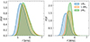 |
Fig. C.1. Posterior distribution of the frequencies at 1 M⊙, 1.4 M⊙ and 2 M⊙ for the p1-mode. The left panel refers to the prescription described in Sec. 5.3 while the right is obtained by inserting the RX(M) relation of each model in (15) with the QU coefficients ai of Sotani (2021). The frequencies in the right panel have a narrower distribution, meaning that the prescription in (17) is necessary to make the spread of our synthetic full GR frequencies similar to the one found by Sotani (2021). |
However, if the relation is only quasi-universal, as manifestly it is the case for the p1-mode shown in Fig. 4, the inversion method will lead to an underestimation of the dispersion of the predictions, and the strategy proposed in Sec. 5.3 should instead be adopted. To check the validity of this statement, we have estimated the distribution of the p1 frequencies in full GR by simply injecting the mass-radius relation RX(M) of the models into the QU relation obtained by Sotani (2021).
The p1-mode distribution obtained in this way – i.e., by “unpacking” the QU relation with RX(M) – is shown in the right panel of Fig. C.1. For each mass, this distribution is narrower than the original spread between the frequencies for different EoS found by Sotani (2021). On the other hand, when we use (17) to transfer the dispersion around the QU relation obtained in Cowling to the full GR prediction (as done in the left panel of Fig. C.1), we qualitatively recover the same spread of frequencies reported in Sotani (2021), after we remove the Shen EoS (Shen et al. 1998) used therein. This EoS is particularly soft and not compatible with the 2.01 M⊙ observation, consequently it cannot be reproduced by our data.
All Tables
All Figures
|
Fig. 1. Probability density distributions for f-mode frequencies (left) and p1-mode frequencies (right), both obtained within the Cowling approximation in the barotropic limit. The three shaded regions refer to the 68%, 95%, and 99% percentiles. The solid black line represents the model with the highest likelihood. |
| In the text | |
|
Fig. 2. Posterior probability density for frequencies of frozen f-mode (upper panel). The lower panel shows the relative difference between the frequencies in the frozen limit and the barotropic limit. The shaded regions represent the 68%, 95%, and 99% percentiles, respectively, while the black line indicates the model with the highest likelihood. |
| In the text | |
|
Fig. 3. Posterior probability density for frequencies of frozen p1 mode (upper panel). The lower panel shows the relative difference between the frequencies in the frozen limit and the barotropic limit. The three shaded regions correspond to the 68%, 95%, and 99% percentiles, while the black line represents the model with the highest likelihood. |
| In the text | |
|
Fig. 4. Relationship between rescaled pulsations ωM and compactness M/R for the frozen f modes (blue-green) and frozen p1 modes (orange-yellow). The dashed lines correspond to the fits presented in Table 1, while the solid black line represents the model ℳ(X) with the highest likelihood ℒ(X). The fit lines overlapping with the distributions are based on the Cowling approximation, whereas the others, obtained in full GR, are shown for comparison. The differences between the rescaled pulsations ωM calculated in the Cowling approximation and the corresponding QU fits are illustrated in the two lower panels. Each panel also includes three shaded regions representing the 68%, 95%, and 99% quantiles of the distribution. |
| In the text | |
|
Fig. 5. Distributions of f-mode frequencies as a function of the average density |
| In the text | |
|
Fig. 6. Probability distributions of synthetic full-GR frequencies obtained from Eq. (17). The left panel shows the f mode, while the right one shows the p1 mode. The three shaded regions in each panel contain the 68%, 95%, and 99% percentiles. The solid black line represents the model with the highest likelihood. |
| In the text | |
|
Fig. 7. Distribution of synthetic full-GR frequencies at 1 M⊙, 1.4 M⊙, and 2 M⊙ obtained from Eq. (17). The left panel refers to the f mode, while the right one refers to the p1 mode. |
| In the text | |
|
Fig. C.1. Posterior distribution of the frequencies at 1 M⊙, 1.4 M⊙ and 2 M⊙ for the p1-mode. The left panel refers to the prescription described in Sec. 5.3 while the right is obtained by inserting the RX(M) relation of each model in (15) with the QU coefficients ai of Sotani (2021). The frequencies in the right panel have a narrower distribution, meaning that the prescription in (17) is necessary to make the spread of our synthetic full GR frequencies similar to the one found by Sotani (2021). |
| In the text | |
Current usage metrics show cumulative count of Article Views (full-text article views including HTML views, PDF and ePub downloads, according to the available data) and Abstracts Views on Vision4Press platform.
Data correspond to usage on the plateform after 2015. The current usage metrics is available 48-96 hours after online publication and is updated daily on week days.
Initial download of the metrics may take a while.