© The Authors 2024

1. Introduction

The detection of the first binary neutron-star (NS) merger by the LIGO-Virgo collaboration (LVC), the event GW170817 (Abbott et al. 2017b), and the associated electromagnetic counterpart (Abbott et al. 2017a,c) has opened a new window to explore matter under extreme conditions. In particular, the imprint on the gravitational-wave (GW) signal left by the tidal interaction of the two NSs during the pre-merger phase led to the first estimate of the tidal deformability (Abbott et al. 2018, 2019), which already made it possible to put some constraints on the properties of dense matter (see Chatziioannou 2020 and references therein for a review). Together with the precise mass determinations of three massive pulsars with masses around 2 M_⊙ – PSR J1614−2230 (Demorest et al. 2010), PSR J0348+0432 (Antoniadis et al. 2013), and PSR J0740+6620 (Cromartie et al. 2020) – as well as the recent quantitative estimations of the mass–radius relation of PSR J0740+6620 and PSR J0030+0451 obtained from the Neutron-star Interior Composition ExploreR (NICER) measurements (Riley et al. 2019, 2021; Raaijmakers et al. 2019; Miller et al. 2019, 2021), these observations advanced the study of the properties of dense matter in NSs. Moreover, the plethora of upcoming observations from the LIGO-Virgo-KAGRA collaboration, as well as those foreseen from the planned third-generation detectors such as the Einstein Telescope (Maggiore 2020; Branchesi et al. 2023) or the Cosmic Explorer (Evans et al. 2021), are expected to provide valuable data from which new information on the structure and composition of NSs can be drawn.

In order to reliably relate different astrophysical observations and extract information both on NS properties and on the dense-matter properties in the interior of NSs, a proper description of the NS equation of state (EoS), that is, the functional relation between the pressure and the mass-energy density, is needed. By ‘proper description’ we mean a consistent mapping of the underlying interaction model on all parts of the internal structure of the star. Indeed, under the assumption of general relativity, the connection between static properties of cold (beta-equilibrated) NSs (which is a valid assumption for mature isolated NSs or coalescing NSs in their inspiral phase such as those considered in this manuscript) and the underlying microphysics mainly relies on the knowledge of the EoS. Most current inferences of NS properties from astrophysical (GW) data are done using agnostic EoSs, that is, EoSs that are not informed by a specific description of the microphysics (they can be parametric – such as piecewise polytropes or sound-speed models – or non-parametric – such as Gaussian processes). These EoSs are usually matched with a (unique) given crust at low densities (typically, the crust of Baym et al. 1971 or of Douchin & Haensel 2001 is used; see e.g., Essick et al. 2020a, 2021; Greif et al. 2019; Huang et al. 2024; Landry & Essick 2019; Raithel & Most 2023a). The reason for this choice is based on the idea that the (low-density) crust EoS is relatively well constrained and that the latter has a negligible effect on NS macroscopic observables, which are instead mainly determined by the largely unknown high-density part of the EoS. However, the determination of the crust EoS, particularly in the inner crust, still suffers from model dependencies (see e.g., Haensel et al. 2007; Oertel et al. 2017; Burgio & Fantina 2018 for a review). In addition, recent studies have shown that an incorrect treatment of the crust and the way the crust is matched to the core EoS can lead to spurious errors in the prediction of the NS macroscopic properties from a given EoS model (see e.g. Fortin et al. 2016; Ferreira & Providência 2020; Suleiman et al. 2021, 2022). These uncertainties are small compared with current precision of astronomical data, but they will become relevant in the near future, in particular for third-generation GW detectors where, for example, the NS radius is expected to be determined to less than 1% precision (see e.g., Chatziioannou 2022; Huxford et al. 2024; Iacovelli et al. 2023). Therefore, it is timely to provide thermodynamically consistent and unified (meaning that the same nuclear model is employed for the different regions of the NSs) EoSs for inference analyses. This is indeed a difficult task since the interior of a NS comprises many different structures from the outer crust with a crystalline structure of ions immersed in an electron gas up to the homogeneous dense core, where large uncertainties on the composition still remain. Each structure thereby needs a specific treatment requiring a consistent matching to obtain a unified description of the entire NS interior.

The large uncertainties at high density in the NS core arise since degrees of freedom other than nucleonic ones can emerge, and phase transitions to quark matter may even occur (see e.g., Haensel et al. 2007; Blaschke & Chamel 2018; Oertel et al. 2017; Raduta 2022 for a review); thus, agnostic models are often used in inference schemes to account for our incomplete knowledge of the high-density EoS. Such phase transitions, however, are unlikely to take place before nuclear saturation density¹ (and even twice saturation density), where only nucleonic degrees of freedom are expected to be present (see e.g., Tang et al. 2021; Christian & Schaffner-Bielich 2020). Therefore, a possible way to build a consistent EoS without losing any freedom in the description of the high-density EoS is to extract the nuclear parameters from the high-density EoS around saturation density, similarly to the procedure proposed in Essick et al. (2021), and subsequently calculate the low-density EoS with the very same parameters. Based on this idea, in this work we propose an efficient way to construct consistent and unified crust–core EoSs of cold and beta-equilibrated NSs for astrophysical (in particular GW signal) analysis.

The formalism is presented in Sect. 2, in which we first discuss in Sect. 2.1 how to extract the nuclear parameters and reconstruct a consistent EoS starting from a relation between the baryon number density and the energy density in beta equilibrium, while we specifically present the framework to calculate the crust EoS in Sect. 2.2 and the global NS properties in Sect. 2.3. Numerical results are given in Sect. 3, in which we first discuss in Sect. 3.1 the procedure and code validation and show the performance of the EoS reconstruction for a limited set of models. To assess the uncertainties associated with the use of a unique crust EoS instead of a consistent model, we perform a Bayesian analysis and systematically compare the predictions of different NS observables predicted by two scenarios: (1) those obtained using a set of crust EoSs matched to (agnostic) polytropic EoSs at high density, and (2) those obtained by employing a unique EoS model at lower densities; results are shown in Sect. 3.2. Finally, we draw our conclusions in Sect. 4.

2. Consistent equation-of-state reconstruction

2.1. Extracting the nuclear-matter parameters from the neutron-star equation of state

Let us suppose that the relation between the energy density of cold beta-equilibrated NS matter ℰ_β and the baryon number density n_B in the zero-temperature approximation is given by an input EoS, not necessarily associated with a specific microscopic model. At a baryonic density low enough that a nucleonic content can safely be assumed (typically less than the saturation density, which corresponds to the internal density of terrestrial atomic nuclei), it is possible to define the energy per baryon of homogeneous nucleonic (neutron, proton, and electron) matter that is consistent with the assumed ℰ_β as²

$$\begin{array}{cc}\hfill e_{\mathrm{nuc},\beta }(n_{\mathrm{B}})& =\frac{1}{n_{\mathrm{B}}}[{\mathcal{E}}_{\beta }(n_{\mathrm{B}})-{\mathcal{E}}_{\mathrm{e}}(n_{\mathrm{e}}(n_{\mathrm{B}}))\hfill \\ \hfill & -n_{\mathrm{e}}{m}_{\mathrm{p}}{c}^2-(n_{\mathrm{B}}-n_{\mathrm{e}})m_{\mathrm{n}}{c}^2],\hfill \end{array}$$(1)

with m_n and m_p being the neutron and proton mass³, respectively, c the speed of light, and n_e the electron density that corresponds to the condition of equilibrium of weak reactions in the nucleonic regime:

$$\begin{array}{c}\hfill {\mu }_{\mathrm{n}}(n_{\mathrm{B}})-{\mu }_{\mathrm{p}}(n_{\mathrm{B}})={\mu }_{\mathrm{e}}(n_{\mathrm{e}}).\end{array}$$(2)

The electron energy density is denoted ℰ_e and given by the expression for an ideal Fermi gas,

$$\begin{array}{c}\hfill {\mathcal{E}}_{\mathrm{e}}=\frac{{(m_{\mathrm{e}}{c}^2)}^4}{8{\pi }^2{(ħc)}^3}[x_r(2x_r^2+1)\sqrt{x_r^2+1}-ln(x_r+\sqrt{x_r^2+1})],\end{array}$$(3)

with x_r = ℏc(3π²n_e)^1/3/(m_ec²) being the relativity parameter, ℏ the Dirac-Planck constant, and m_e the electron mass (see e.g. Weiss et al. 2004). We note that in principle muons can contribute to the EoS, thus to ℰ_β. However, in Eq. (1) we only consider electrons since muons are not expected to contribute before saturation density; therefore, the procedure of the extraction of the nuclear-matter parameters described here remains valid. The isospin asymmetry parameter is denoted as δ and defined using the neutron and proton number density, n_n and n_p, respectively, as δ = (n_n − n_p)/n_B. For a pure nucleonic content, the value of the isospin asymmetry at each density, δ_β(n_B), is related to the electron number density by the charge neutrality condition n_e = n_B (1 − δ_β)/2.

In order to build a consistent description of the crust with standard variational tools, as pioneered by Baym et al. (1971) and Douchin & Haensel (2001), one needs to know the behaviour of e_nuc for different values of 0 < δ < 1 besides the β-equilibrium value δ_β(n_B) in the sub-saturation density regime. To this aim, we write the energy density of nucleonic matter using the following expression, as in the meta-model approach developed in Margueron et al. (2018):

$$\begin{array}{c}\hfill {\mathcal{E}}_{\mathrm{nuc}}(n_{\mathrm{B}},\delta )=\sum _{q=n,p}{n}_q{m}_q{c}^2+n_{\mathrm{B}}{e}_{\mathrm{nuc}}(n_{\mathrm{B}},\delta ),\end{array}$$(4)

where q = n, p labels neutron and proton, respectively, and the energy per baryon is given by

$$\begin{array}{c}\hfill e_{\mathrm{nuc}}(n_{\mathrm{B}},\delta )=t_{\mathrm{FG}}^{\star }(n_{\mathrm{B}},\delta )+e_{\mathrm{is}}(n_{\mathrm{B}})+e_{\mathrm{iv}}(n_{\mathrm{B}}){\delta }^2,\end{array}$$(5)

where e_is(n_B) (e_iv(n_B)) is the isoscalar (isovector) energy (see Eq. (16) and the following). We note that Eq. (5) is not a purely parabolic approximation for the isospin dependence because of the kinetic term $t_{\text{FG}}^{\star }$, which includes the dominant deviation to the parabolic approximation,

$$\begin{array}{cc}\hfill t_{\mathrm{FG}}^{\star }(n,\delta )& =\frac{t_{\mathrm{FG},\mathrm{sat}}}{2}{\left(\frac{n_{\mathrm{B}}}{n_{\mathrm{sat}}}\right)}^{2/3}[(1+{\kappa }_{\mathrm{sat}}\frac{n_{\mathrm{B}}}{n_{\mathrm{sat}}})f_1(\delta )\hfill \\ \hfill & +{\kappa }_{\mathrm{sym}}\frac{n_{\mathrm{B}}}{n_{\mathrm{sat}}}{f}_2(\delta )],\hfill \end{array}$$(6)

where $t_{\mathrm{FG},\mathrm{sat}}=3{ħ}^2{c}^2{(3{\pi }^2/2)}^{2/3}{n}_{\mathrm{sat}}^{2/3}/(10m{c}^2)$ is the kinetic energy per nucleon of symmetric nuclear matter at the saturation density n_sat, with m = (m_n + m_p)/2, and the functions f_i are defined as

$$\begin{array}{cc}& f_1(\delta )={(1+\delta )}^{5/3}+{(1-\delta )}^{5/3},\hfill \end{array}$$(7)

$$\begin{array}{cc}& f_2(\delta )=\delta [{(1+\delta )}^{5/3}-{(1-\delta )}^{5/3}].\hfill \end{array}$$(8)

The terms κ_sat and κ_sym in Eq. (6) are linked to the nucleon effective masses $m_q^{\star }$ by

$$\begin{array}{cc}& {\kappa }_{\mathrm{sat}}=\frac{m}{m_{\mathrm{sat}}^{\star }}-1\mathrm{in}\mathrm{symmetric}\mathrm{matter}(\delta =0),\hfill \\ \hfill & {\kappa }_{\mathrm{sym}}=\frac{1}{2}[\frac{m}{m_{\mathrm{n}}^{\star }}-\frac{m}{m_{\mathrm{p}}^{\star }}]\mathrm{in}\mathrm{neutron}\mathrm{matter}(\delta =1),\hfill \end{array}$$(9)

where $m_{\text{sat}}^{\star }=m^{\star }(n_{\text{sat}})$ is the Landau effective mass at saturation (see also the discussion in Margueron et al. 2018). In order to equate Eqs. (1) and (5) along the beta-equilibrium curve δ = δ_β(n_B), the chemical potentials have to be computed. The electron chemical potential is simply given by its Fermi energy,

$$\begin{array}{c}\hfill {\mu }_{\mathrm{e}}=\sqrt{{(ħc)}^2{(3{\pi }^2{n}_{\mathrm{e}})}^{2/3}+{(m_{\mathrm{e}}{c}^2)}^2},\end{array}$$(10)

and the neutron and proton chemical potentials are given by

$$\begin{array}{c}\hfill {\mu }_q={\frac{\partial {\mathcal{E}}_{\mathrm{nuc}}}{\partial n_q}|}_{n_{q^{\prime }}}=e_{\mathrm{nuc}}+m_q{c}^2+{n_{\mathrm{B}}\frac{\partial e_{\mathrm{nuc}}}{\partial n_{\mathrm{B}}}|}_{\delta }+(-\delta \pm 1){\frac{\partial e_{\mathrm{nuc}}}{\partial \delta }|}_{n_{\mathrm{B}}},\end{array}$$(11)

where the plus (minus) sign holds for neutrons (protons). Replacing Eq. (11) in Eq. (2), we obtain the standard beta-equilibrium condition (see Lattimer et al. 1991; Li et al. 1998):

$$\begin{array}{c}\hfill 2{\frac{\partial e_{\mathrm{nuc}}}{\partial \delta }|}_{n_{\mathrm{B}}}(n_{\mathrm{B}},{\delta }_{\beta })={\mu }_{\mathrm{e}}(n_{\mathrm{B}},{\delta }_{\beta })-\mathrm{\Delta }{m}_{\mathrm{np}}{c}^2,\end{array}$$(12)

with Δm_np = m_n − m_p, or equivalently, using the expansion in Eq. (5),

$$\begin{array}{c}\hfill 2{\frac{\partial t_{\mathrm{FG}}^{\star }}{\partial \delta }|}_{n_{\mathrm{B}}}(n_{\mathrm{B}},{\delta }_{\beta })-{\mu }_{\mathrm{e}}(n_{\mathrm{B}},{\delta }_{\beta })+\mathrm{\Delta }{m}_{\mathrm{np}}{c}^2=-4{\delta }_{\beta }{e}_{\mathrm{iv}}(n_{\mathrm{B}}).\end{array}$$(13)

The unknown density-dependent isovector energy e_iv(n_B) in Eq. (13) can be extracted from the input ℰ_β(n_B) using Eqs. (1) and (5):

$$\begin{array}{cc}\hfill {\delta }_{\beta }^2{e}_{\mathrm{iv}}(n_{\mathrm{B}})& =\frac{1}{n_{\mathrm{B}}}[{\mathcal{E}}_{\beta }(n_{\mathrm{B}})-{\mathcal{E}}_{\mathrm{e}}(n_{\mathrm{e}})\hfill \\ \hfill & -n_{\mathrm{e}}{m}_{\mathrm{p}}{c}^2-(n_{\mathrm{B}}-n_{\mathrm{e}})m_{\mathrm{n}}{c}^2]\hfill \\ \hfill & -t_{\mathrm{FG}}^{\star }(n_{\mathrm{B}},{\delta }_{\beta })-e_{\mathrm{is}}(n_{\mathrm{B}}).\hfill \end{array}$$(14)

Replacing Eq. (14) in Eq. (13), we have

$$\begin{array}{cc}& 2{\frac{\partial t_{\mathrm{FG}}^{\star }}{\partial \delta }|}_{n_{\mathrm{B}}}(n_{\mathrm{B}},{\delta }_{\beta })-{\mu }_{\mathrm{e}}(n_{\mathrm{B}},{\delta }_{\beta })+\mathrm{\Delta }{m}_{\mathrm{np}}{c}^2\hfill \\ \hfill & =-\frac{4}{n_{\mathrm{B}}{\delta }_{\beta }}[{\mathcal{E}}_{\beta }(n_{\mathrm{B}})-{\mathcal{E}}_{\mathrm{e}}(n_{\mathrm{e}})\hfill \\ \hfill & -n_{\mathrm{e}}{m}_{\mathrm{p}}{c}^2-(n_{\mathrm{B}}-n_{\mathrm{e}})m_{\mathrm{n}}{c}^2\hfill \\ \hfill & -n_{\mathrm{B}}{t}_{\mathrm{FG}}^{\star }(n_{\mathrm{B}},{\delta }_{\beta })-n_{\mathrm{B}}{e}_{\mathrm{is}}(n_{\mathrm{B}})].\hfill \end{array}$$(15)

For each value of n_B, this equation can be numerically solved for δ_β, as proposed by Essick et al. (2021); the expression is slightly more involved because of the explicit inclusion of the kinetic term in Eq. (5), but the numerical complexity is the same as for Eq. (22) in Essick et al. (2021).

The solution of Eq. (15) requires knowledge of the isoscalar energy functional e_is(n_B). A simple harmonic approximation (Essick et al. 2021) is correct around saturation, but it is not sufficient (see e.g. Fig. 5 in Margueron et al. 2018) if one wants to extract the behaviour of the functional at very low density, which is the domain better constrained by the ab initio calculations, and it is also very important for a correct calculation of the crust (Dinh Thi et al. 2021a). We then used the meta-model labelled ‘ELFc’ in Margueron et al. (2018), truncated at order N. It was shown that, when truncating the expansion at order N = 4 (and even N = 3), the meta-model gives a very good reproduction of realistic functionals at low density (see Margueron et al. 2018 and Sect. 3.1 for a discussion on the truncation order). Defining x = (n_B − n_sat)/(3n_sat), we write:

$$\begin{array}{c}\hfill e_{\mathrm{is}}(n_{\mathrm{B}})=\sum _{k=0}^N\frac{v_k^{\mathrm{is}}}{k!}{x}^k{u}_k(x),\end{array}$$(16)

where the function u_k,

$$\begin{array}{c}\hfill u_k(x)=1-{(-3x)}^{N+1-k}{e}^{-b{n}_{\mathrm{B}}/n_{\mathrm{sat}}}\end{array}$$(17)

with b = 10ln2 (Margueron et al. 2018), ensures the correct zero-density limit, and the parameters $v_i^{\text{is}}$ are directly connected to the so-called isoscalar nuclear empirical parameters. At order N = 4 we obtain the following:

$$\begin{array}{cc}& v_0^{\mathrm{is}}=E_{\mathrm{sat}}-t_{\mathrm{FG},\mathrm{sat}}(1+{\kappa }_{\mathrm{sat}}),\hfill \end{array}$$(18)

$$\begin{array}{cc}& v_1^{\mathrm{is}}=-t_{\mathrm{FG},\mathrm{sat}}(2+5{\kappa }_{\mathrm{sat}}),\hfill \end{array}$$(19)

$$\begin{array}{cc}& v_2^{\mathrm{is}}=K_{\mathrm{sat}}-2t_{\mathrm{FG},\mathrm{sat}}(5{\kappa }_{\mathrm{sat}}-1),\hfill \end{array}$$(20)

$$\begin{array}{cc}& v_3^{\mathrm{is}}=Q_{\mathrm{sat}}-2t_{\mathrm{FG},\mathrm{sat}}(4-5{\kappa }_{\mathrm{sat}}),\hfill \end{array}$$(21)

$$\begin{array}{cc}& v_4^{\mathrm{is}}=Z_{\mathrm{sat}}-8t_{\mathrm{FG},\mathrm{sat}}(-7+5{\kappa }_{\mathrm{sat}}).\hfill \end{array}$$(22)

Once the isoscalar parameters at order N (E_sat, K_sat, Q_sat, Z_sat for N = 4) are picked, Eq. (15) is solved for N + 1 different sub-saturation density points, n_B, j, corresponding to N + 1 points – x_j, j = 1…N + 1 – which have to be defined. The isovector empirical parameters (E_sym, L_sym, K_sym, Q_sym, Z_sym for N = 4) can thus be analytically obtained by matrix inversion (Mondal & Gulminelli 2022):

$$\begin{array}{c}\hfill \left|\begin{array}{c}{E}_{\mathrm{sym}}\\ L_{\mathrm{sym}}\\ K_{\mathrm{sym}}\\ Q_{\mathrm{sym}}\\ Z_{\mathrm{sym}}\end{array}\right|={\left|\begin{array}{ccccc}{U}_{01}& x_1{U}_{11}& \frac{x_1^2}{2}{U}_{21}& \frac{x_1^3}{6}{U}_{31}& \frac{x_1^4}{24}{U}_{41}\\ U_{02}& x_2{U}_{12}& \frac{x_2^2}{2}{U}_{22}& \frac{x_2^3}{6}{U}_{32}& \frac{x_2^4}{24}{U}_{42}\\ U_{03}& x_3{U}_{13}& \frac{x_3^2}{2}{U}_{23}& \frac{x_3^3}{6}{U}_{33}& \frac{x_3^4}{24}{U}_{43}\\ U_{04}& x_4{U}_{14}& \frac{x_4^2}{2}{U}_{24}& \frac{x_4^3}{6}{U}_{34}& \frac{x_4^4}{24}{U}_{44}\\ U_{05}& x_5{U}_{15}& \frac{x_5^2}{2}{U}_{25}& \frac{x_5^3}{6}{U}_{35}& \frac{x_5^4}{24}{U}_{45}\end{array}\right|}^{-1}\left|\begin{array}{c}{e}_{\mathrm{iv}}^1\\ e_{\mathrm{iv}}^2\\ e_{\mathrm{iv}}^3\\ e_{\mathrm{iv}}^4\\ e_{\mathrm{iv}}^5\end{array}\right|,\end{array}$$(23)

with U_nk = u_n(x_k) and

$$\begin{array}{cc}\hfill e_{\mathrm{iv}}^k& =e_{\mathrm{iv}}(x_k)+\frac{5}{9}{U}_{0k}{t}_{\mathrm{FG},\mathrm{sat}}[1+({\kappa }_{\mathrm{sat}}+3{\kappa }_{\mathrm{sym}})]\hfill \\ \hfill & +\frac{5}{9}{x}_k{U}_{1k}{t}_{\mathrm{FG},\mathrm{sat}}[2+5({\kappa }_{\mathrm{sat}}+3{\kappa }_{\mathrm{sym}})]\hfill \\ \hfill & +\frac{10}{9}\frac{x_k^2}{2}{U}_{2k}{t}_{\mathrm{FG},\mathrm{sat}}[-1+5({\kappa }_{\mathrm{sat}}+3{\kappa }_{\mathrm{sym}})]\hfill \\ \hfill & +\frac{10}{9}\frac{x_k^3}{6}{U}_{3k}{t}_{\mathrm{FG},\mathrm{sat}}[4-5({\kappa }_{\mathrm{sat}}+3{\kappa }_{\mathrm{sym}})]\hfill \\ \hfill & +\frac{40}{9}\frac{x_k^4}{24}{U}_{4k}{t}_{\mathrm{FG},\mathrm{sat}}[-7+5({\kappa }_{\mathrm{sat}}+3{\kappa }_{\mathrm{sym}})].\hfill \end{array}$$(24)

This ‘inversion procedure’ thus allows one to extract the nucleonic functional e_nuc(n_B, δ) (see Eqs. (1) and (5)) from a given beta-equilibrated EoS ℰ_β(n_B) and a set of isoscalar parameters⁴. All isoscalar and isovector parameters being known, the crust EoS and the crust–core transition point are calculated from the crust code originally described in Carreau et al. (2019a), Dinh Thi et al. (2021b,c; see Sect. 2.2).

A first application of this method consists of assigning specific values of the isoscalar empirical parameter corresponding to those of given nuclear models, which allows one to reconstruct the isovector parameters when not known at the same order as the isoscalar ones; with this set of parameters, it is thus possible to compute a unified EoS. This is of particular interest for EoSs that have only been computed for the core (e.g., EoSs based on microscopic approaches not yet available for the crust), thus allowing for a unified treatment of all the regions of the NS. Results for this application are discussed in Sect. 3.1.

A second and wider application of this approach is connected to Bayesian inference from GW data for which agnostic EoSs are often used. Indeed, for each agnostic realisation ℰ_β(n_B), it is possible to sample the values of the (unknown) parameters $(n_{\text{sat}},E_{\text{sat}},K_{\text{sat}},Q_{\text{sat}},m_{\text{sat}}^{\star },\mathrm{\Delta }{m}_{\text{sat}}^{\star })$, and eventually Z_sat for an order-4 reconstruction, from flat (or gaussian) distributions in the following range (Dinh Thi et al. 2021c):

$$\begin{array}{cc}& n_{\mathrm{sat}}=0.16\pm 0.01{\mathrm{fm}}^{-3}\hfill \end{array}$$(25)

$$\begin{array}{cc}& E_{\mathrm{sat}}=-16.00\pm 1.00\mathrm{MeV}\hfill \end{array}$$(26)

$$\begin{array}{cc}& K_{\mathrm{sat}}=230\pm 40\mathrm{MeV}\hfill \end{array}$$(27)

$$\begin{array}{cc}& Q_{\mathrm{sat}}=0.0\pm 1000.0\mathrm{MeV}\hfill \end{array}$$(28)

$$\begin{array}{cc}& Z_{\mathrm{sat}}=0.0\pm 3000.0\mathrm{MeV}\hfill \end{array}$$(29)

$$\begin{array}{cc}& m_{\mathrm{sat}}^{\star }/m=0.7\pm 0.1\hfill \end{array}$$(30)

$$\begin{array}{cc}& \mathrm{\Delta }{m}_{\mathrm{sat}}^{\star }/m=(m_{\mathrm{n}}^{\star }-m_{\mathrm{p}}^{\star })/m=0.1\pm 0.1.\hfill \end{array}$$(31)

Once the isoscalar parameters are picked, and for each sub-saturation density point x_j, Eq. (14) gives e_iv(n_B) and, consequently, the neutron energy e_nuc(n_B, 1) from Eq. (5). The model can thus be filtered through chiral effective field theory (EFT) calculations (see Sect. 3.2). If retained, the isovector parameters can be calculated via Eq. (23); thus, a consistent and unified crust–core EoS can be constructed.

2.2. Crust equation of state

The crust EoS is calculated as described in Carreau et al. (2019a) (see also Dinh Thi et al. 2021a,b,c) within a compressible liquid-drop (CLD) model approach. Although not as microscopic as a full density functional treatment, this method was recently shown to provide results in good agreement with extended Thomas-Fermi calculations both at zero (Grams et al. 2022) and at finite temperature Carreau et al. (2020; see also Fig. 2 in Carreau et al. 2019a for an illustration of the performance of the CLD model we used to reproduce experimental masses). Moreover, it makes it possible to quantitatively estimate the model dependence of the results by comparing different EoS models at a reduced computational cost. We only recall the main points of this method here for completeness. Because of the zero-temperature approximation, we employ the one-component plasma approach, that is, we consider one nuclear cluster at each (increasing) density in the crust for the composition. At each layer of the crust, characterised by a pressure P and baryon density n_B, matter is modelled as a periodic lattice consisting of Wigner-Seitz cells of volume V_WS containing one type of cluster with Z protons of mass m_p and A − Z neutrons of mass m_n (A being the cluster total mass number), immersed in a uniform gas of electrons and, in the inner crust, of neutrons too. For a given thermodynamic condition, defined by the baryonic density n_B, the total energy density of the inhomogeneous system can thus be written as

$$\begin{array}{c}\hfill {\mathcal{E}}_{\mathrm{inhom}}={\mathcal{E}}_{\mathrm{e}}+{\mathcal{E}}_{\mathrm{g}}(1-u)+\frac{E_{\mathrm{i}}}{V_{\mathrm{WS}}},\end{array}$$(32)

where ℰ_e(n_e) is the electron gas energy density, ℰ_g = ℰ_nuc(n_g, δ_g) is the neutron-gas energy density (including the rest masses of nucleons) at baryonic density n_g = n_gn and isospin asymmetry δ_g = 1 (no protons are present in the gas), and $u=\frac{A/n_{\mathrm{i}}}{V_{\mathrm{WS}}}$ is the volume fraction of the cluster with internal density n_i. Finally, the third term on the right hand side of Eq. (32), −ℰ_gu, accounts for the interaction between the cluster and the neutron gas, that we treated in the excluded-volume approach. In the outer crust, ℰ_g is set to zero. The last term in Eq. (32) is the cluster energy per Wigner-Seitz cell:

$$\begin{array}{c}\hfill E_{\mathrm{i}}=M_{\mathrm{i}}{c}^2+E_{\mathrm{bulk}}+E_{\mathrm{Coul}}+E_{\mathrm{surf}+\mathrm{curv}},\end{array}$$(33)

where M_i = (A − Z)m_n + Zm_p is the total bare mass of the cluster, E_bulk = Ae_nuc(n_i, 1 − 2Z/A) is the cluster bulk energy, and E_Coul + E_{surf + curv} = V_WS(ℰ_Coul + ℰ_{surf + curv}) accounts for the total interface energy, that is, the Coulomb interaction between the nucleus and the electron gas, as well as the residual interface interaction between the nucleus and the surrounding dilute nuclear-matter medium. For the bulk energy density of the ions – ℰ_bulk = e_nucn_i – and that of the neutron gas, we use the same functional expression, that is, the meta-model approach of Margueron et al. (2018; see Eq. (4)). We consider here only spherical clusters, since the so-called pasta phases that may appear at the bottom of the inner crust are expected to have only a small impact on the EoS; therefore, the Coulomb energy density is given by

$$\begin{array}{c}\hfill {\mathcal{E}}_{\mathrm{Coul}}=\frac{2}{5}\pi {(e{n}_{\mathrm{i}}{r}_N)}^{2}u{\left(\frac{1-I}{2}\right)}^2[u+2(1-\frac{3}{2}{u}^{1/3})],\end{array}$$(34)

with e being the elementary charge, I = 1 − 2Z/A, and r_N = (3A/(4πn_i))^1/3. For the surface and curvature contributions, we employed the same expression as in Maruyama et al. (2005) and Newton et al. (2013), that is

$$\begin{array}{c}\hfill {\mathcal{E}}_{\mathrm{surf}}+{\mathcal{E}}_{\mathrm{curv}}=\frac{3u}{r_N}({\sigma }_{\mathrm{s}}(I)+\frac{2{\sigma }_{\mathrm{c}}(I)}{r_N}),\end{array}$$(35)

where σ_s and σ_c are the surface and curvature tensions (Ravenhall et al. 1983), and

$$\begin{array}{cc}& {\sigma }_{\mathrm{s}}(I)={\sigma }_0\frac{2^{p+1}+b_{\mathrm{s}}}{y_{\mathrm{p}}^{-p}+b_{\mathrm{s}}+{(1-y_{\mathrm{p}})}^{-p}},\hfill \end{array}$$(36)

$$\begin{array}{cc}& {\sigma }_{\mathrm{c}}(I)=5.5{\sigma }_{\mathrm{s}}(I)\frac{{\sigma }_{0,\mathrm{c}}}{{\sigma }_0}(\beta -y_{\mathrm{p}}),\hfill \end{array}$$(37)

where y_p = (1 − I)/2 and the surface parameters (σ₀, σ_0, c, b_s, β) were optimised for each set of bulk parameters and effective mass to reproduce the experimental nuclear masses in the 2020 Atomic Mass Evaluation (AME) table (Wang et al. 2021), while we set p = 3. The EoS and composition of the crust was then obtained by variationally minimising the energy density of the Wigner–Seitz cell with (A, I, n_i, n_e, n_g) as variational variables, under the constraint of baryon number conservation and charge neutrality holding in every cell (Carreau et al. 2019a; Dinh Thi et al. 2021a,b).

2.3. Global neutron-star properties

Once the EoSs P(ℰ) are generated, the properties of a static NS are calculated from the Tolman–Oppenheimer–Volkoff (TOV) equations (Tolman 1939; Oppenheimer & Volkoff 1939):

$$\begin{array}{cc}\hfill \frac{\mathrm{d}P(r)}{\mathrm{d}r}& =-\frac{G\mathcal{E}(r)\mathcal{M}(r)}{c^2{r}^2}[1+\frac{P(r)}{\mathcal{E}(r)}]\hfill \\ \hfill & \times [1+\frac{4\pi P(r)r^3}{c^2\mathcal{M}(r)}][1-\frac{2G\mathcal{M}(r)}{c^{2}r}{]}^{-1},\hfill \end{array}$$(38)

with ℰ being the total energy density of the (beta-equilibrated) system and

$$\begin{array}{c}\hfill \mathcal{M}(r)=\frac{4\pi }{c^2}{\int }_0^r\mathcal{E}(r^{\prime })r{\prime }^2\mathrm{d}{r}^{\prime }.\end{array}$$(39)

The integration of Eqs. (38)–(39) until the surface of the star defines its radius R and mass M = ℳ(r = R). In addition, the dimensionless tidal deformability Λ = λ(r = R) is calculated as

$$\begin{array}{c}\hfill \lambda (r)=\frac{2}{3}{k}_2(r){\left[\frac{r{c}^2}{G\mathcal{M}(r)}\right]}^5,\end{array}$$(40)

with the tidal Love number function k₂(r) given by (Hinderer 2008; Hinderer et al. 2010)

$$\begin{array}{cc}\hfill k_2& =\frac{8C^5}{5}{(1-2C)}^2[2+2C(y-1)-y]\hfill \\ \hfill & \times \{2C[6-3y+3C(5y-8)]\hfill \\ \hfill & +4C^3[13-11y+C(3y-2)+2C^2(1+y)]\hfill \\ \hfill & +3{(1-2C)}^2[2-y+2C(y-1)]ln(1-2C){\}}^{-1},\hfill \end{array}$$(41)

where we introduce the dimensionless compactness parameter

$$\begin{array}{c}\hfill C(r)=\frac{G\mathcal{M}(r)}{r{c}^2},\end{array}$$(42)

and the function y(r) is obtained by integrating the following differential equation with the boundary condition y(0) = 2:

$$\begin{array}{cc}& r\frac{\mathrm{d}y}{\mathrm{d}r}+y{(r)}^2+F(r)y(r)+Q(r)=0,\hfill \end{array}$$(43)

$$\begin{array}{cc}& F(r)=\frac{1-4\pi G{r}^2(\mathcal{E}(r)-P(r))/c^4}{1-2G\mathcal{M}(r)/(r{c}^2)},\hfill \end{array}$$(44)

$$\begin{array}{cc}& Q(r)=\frac{4\pi G{r}^2/c^4}{1-2G\mathcal{M}(r)/(r{c}^2)}[5\mathcal{E}(r)+9P(r)\hfill \\ \hfill & +\frac{\mathcal{E}(r)+P(r)}{c_s{(r)}^2}{c}^2-\frac{6c^4}{4\pi r^{2}G}]\hfill \\ \hfill & -4[\frac{G(\mathcal{M}(r)/(r{c}^2)+4\pi r^{2}P(r)/c^4)}{1-2G\mathcal{M}(r)/(r{c}^2)}{]}^2,\hfill \end{array}$$(45)

with $c_{\mathrm{s}}=c\sqrt{\mathrm{d}P/\mathrm{d}\mathcal{E}}$ denoting the sound speed.

We also recall that the effective tidal deformability $\stackrel{\sim }{\mathrm{\Lambda }}$ of the binary, which can be extracted from GW measurements, is expressed in the form of the component masses, m₂ ≤ m₁, and the two corresponding dimensionless tidal deformabilities, Λ₁ = λ₁(R₁) and Λ₂ = λ₂(R₂), as

$$\begin{array}{c}\hfill \stackrel{\sim }{\mathrm{\Lambda }}=\frac{16}{13}\frac{(m_1+12m_2)m_1^4{\mathrm{\Lambda }}_1+(m_2+12m_1)m_2^4{\mathrm{\Lambda }}_2}{{(m_1+m_2)}^5},\end{array}$$(46)

while the chirp mass associated with a binary system reads

$$\begin{array}{c}\hfill {\mathcal{M}}_{\mathrm{c}}=\frac{{(m_1{m}_2)}^{3/5}}{{(m_1+m_2)}^{1/5}}=\frac{q^{3/5}{m}_1}{{(1+q)}^{1/5}},\end{array}$$(47)

with q = m₂/m₁ being the mass ratio.

3. Numerical results

In this section, we present the results obtained using the Crust (Unified) Tool for Equation-of-state Reconstruction (CUTER) code⁵, based on the method described in Sect. 2. We point out that the reconstructed EoS is only valid until around saturation density, where the density points n_B, j are chosen. The final EoS is then built by matching the reconstructed EoS to the original one either at the crust–core transition or until the first point in the original (high-density) EoS table, if the latter is after the crust–core transition. However, since the nuclear empirical parameters used for the crust are consistent with those used for the core EoS around saturation density, a continuous and smooth behaviour in the energy density is ensured.

3.1. Code validation

In order to validate the procedure, we start by considering known beta-equilibrated EoSs, namely the PCP(BSk24) (Pearson et al. 2018, 2019), the RG(SLy4) (Gulminelli & Raduta 2015), the GPPVA(DDME2) (Grill et al. 2012, 2014), and the GPPVA(TW) (Grill et al. 2014) ones, available on the CompOSE database⁶ (Typel et al. 2015; CompOSE Core Team 2022). They are based on the BSk24 (Goriely et al. 2013), the SLy4 (Chabanat et al. 1997), the DDME2 (Lalazissis et al. 2005), and the TW99 (Typel & Wolter 1999) energy-density functionals, respectively. The choice of these models was driven by the fact that they span different values of the nuclear-matter parameters, which are consistent with current knowledge of nuclear physics, and they all yield EoSs that are able to support 2 M_⊙ NSs. Finally, the corresponding nuclear empirical parameters up to order N = 4 (see Table 2) are available for these functionals (Margueron et al. 2018; Dinh Thi et al. 2021a), so different orders of the reconstruction can be tested. Although we only show a limited number of models here, as illustrative examples, we performed code validation and automated tests on a larger set of available EoSs.

We start by fixing the isoscalar parameters as those characterising the corresponding functional⁷ and N points in density, n_B, j, around saturation (N being the order of the reconstruction; see Table 1). The isovector parameters are then calculated using the inversion procedure described in Sect. 2 (see Eq. (23)). We emphasise that the obtained parameter values, and thus the EoS reconstruction, may depend on the choice of the density points n_B, j. However, the impact on NS macroscopic properties such as the mass–radius relation remains small, as long as the original (input) EoS covers a baryon density range that does not require considerable extrapolation to obtain the EoS at the chosen n_B, j required for the reconstruction at a given order N.

To evaluate the quality of the reconstruction, we start by listing the nuclear empirical parameters for the four considered models in Table 2: the first line corresponds to the parameter set of the original model, while the following lines indicate the (input) isoscalar parameters and the reconstructed isovector ones for different orders of the reconstruction. We can see that the inversion procedure yields a good reproduction of the low-order parameters, while larger deviations are observed for the high-order ones. This can be understood from the fact that the reconstruction requires us to fix a number of given points in density (see Table 1), chosen around and below saturation. In this density regime, the contribution of the high-order terms is almost negligible; thus, the discrepancies in the high-order terms arise from the capability of the polynomial expansion to reproduce the functional behaviour (thus to recover the higher order parameters) when extrapolated far below or above saturation. However, the NS mass–radius relation is only slightly impacted since it is dominated by the high-density part, where in any case the original EoS is matched.

With the complete set of parameters, we first calculate the EoS of pure neutron matter and symmetric matter. The correct reproduction of the homogeneous matter is particularly important when performing Bayesian analyses since the chiral-EFT filter, which indeed operates on homogeneous matter, can be applied to discriminate models. In Fig. 1, we show the energy per baryon of symmetric nuclear matter (left panels) and pure neutron matter (right panels) for the BSk24 (top panels) and TW99 (bottom panels) models as illustrative examples; the dots are obtained with the full parameter set of the original model, while the dotted, dash-dotted, and solid curves correspond to the results obtained with the reconstruction at order 2, 3, and 4, respectively. We can see that for the symmetric sector (left panels) the reconstruction is very close to the original model, with a slight deviation at very low density for the reconstructions at order 2. This is somehow expected since only the isoscalar parameters enter in the determination of the symmetric-matter energy (see Eqs. (5), (18)–(22)), and these are fixed as input. The small deviation observed can therefore be attributed to the capability of the meta-model truncated at a given order to reproduce the original functional (see also the discussion in Margueron et al. 2018). On the other hand, in the calculation of the pure neutron-matter energy, the isovector parameters, which are calculated through the inversion procedure in Eq. (23), play an important role. Since the reconstruction gives values of the isovector parameters close to those of the original model but not exactly identical, deviations can appear far from saturation density (i.e., away from the chosen n_B, j points in density; see Table 1). This is observed, for the considered cases, for the order-2 reconstruction for TW99 at very low density, where high-order parameters can also be influential (see lower right panel of Fig. 1), while the inversion procedure yields a very good reconstruction at any order for BSk24 (upper right panel of Fig. 1). For comparison, we also show the band of the chiral-EFT calculations of Drischler et al. (2016; orange shaded area). It is interesting to see that the reproduction of the original model is, in both of the shown cases (and for all EoS models that we tested), very precise at order 4 in spite of the relatively poor reconstruction of the isovector nuclear-matter parameters shown in Table 2. This underlines the fact that significant degeneracy exists in the nuclear-empirical-parameter space, and caution should be taken when attributing specific physical effects to individual parameters, particularly of order 2 or higher. We also note that the quality of the reconstruction depends on the original input EoS as well (density grid, numerical precision, etc.), and thus on the numerical computation of the EoS.

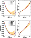Fig. 1. Energy per baryon versus baryon number density for symmetric nuclear matter (SNM; left panels) and for pure neutron matter (PNM; right panels), for the BSk24 (top panels) and the TW99 (bottom panels) models. Dots correspond to the results obtained using the original set of isoscalar and isovector parameters, while dotted blue lines, dash-dotted green lines, and solid red lines correspond to the results from the reconstruction at order 2, 3, and 4, respectively. For comparison, the chiral-EFT calculations of Drischler et al. (2016) are also shown (yellow bands; see text for details).

We now discuss the beta-equilibrium EoS calculated with the parameter sets reconstructed at different orders and its impact on (global) NS properties. In Fig. 2 we display the EoS (left panels), the resulting mass-radius relation (middle panels), and the relative absolute error on the radius (right panels) for the BSk24 (top panels) and TW99 (bottom panels) models with respect to that obtained using the original EoS tables. We can see that the EoS is reconstructed with very good accuracy, and the mass-radius curves are almost indistinguishable. Instead, it might be surprising that the order-2 EoS, which generally does not yield the most accurate reconstruction, gives instead the lowest error on the radius in some cases, but this might be also due to the numerical interpolation of the EoS table in the TOV solver used. In any case, the relative error on the radius remains very small: ≲0.5% in all cases considered here.

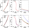Fig. 2. Pressure versus baryon number density (left panels), mass-radius relation (middle panels), and absolute relative error on the radius (right panels) for different models. Crosses and solid black lines (left and middle panel, respectively) correspond to the original EoS, while dotted blue lines, dash-dotted green lines, and solid red lines correspond to the reconstruction at order 2, 3, and 4, respectively (see text for details).

Of particular importance for the NS modelling, and specifically for observables related to the crust physics, is the crust–core transition. In Table 3, we list the crust–core transition density and pressure for the four considered models, as indicated in the ‘original’ EoS tables (Pearson et al. 2018; Douchin & Haensel 2001; Grill et al. 2014) and as predicted by the EoSs reconstructed at different orders. We can see that the reconstruction procedure also gives very good predictions for the crust–core transition, the order-4 (order-2) EoS generally being the one yielding the better (worse) agreement with the values obtained in the original models. These results can be deemed as satisfactory, especially considering that the exact value of crust–core transition pressure and density are known to depend not only on the EoS, but also on the many-body method used to determine it. An example of this latter dependence can be seen by comparing the RG(SLy4) (Gulminelli & Raduta 2015) and the DH(SLy4) (Douchin & Haensel 2001) EoSs, both based on the SLy4 functional; indeed, the crust–core transition density and pressure predicted by the RG(SLy4) EoS are n_cc = 0.052 fm⁻³ and P_cc = 0.16 MeV fm⁻³, respectively, to be compared with the values reported in Douchin & Haensel (2001), namely, n_cc = 0.076 fm⁻³ and P_cc = 0.34 MeV fm⁻³.

These results show that the inversion procedure can be applied to different models for the EoS, thus allowing the reconstruction of the crust and core EoS in a consistent and unified way. In order to evaluate the impact on the global NS properties of using such unified EoSs against a unique crust model, we performed a Bayesian analysis, as described in the next section.

3.2. Bayesian analysis

To assess the uncertainties associated with the crust EoS, we performed a Bayesian analysis. The nuclear meta-modelling is run at order N = 4 up to a given baryon density n_match, and the nuclear empirical parameters {n_sat, E_sat, sym, L_sym, K_sat, sym, Q_sat, sym, Z_sat, sym}, together with the nucleon effective mass $m_{\text{sat}}^{\star }/m$ and effective mass isosplit $\mathrm{\Delta }{m}_{\text{sat}}^{\star }/m$, are sampled from a uniform non-informative prior (see Table 4), as was done, for example, in Dinh Thi et al. (2021c). In addition, for the present analysis, the b parameter governing the low-density limit (see Eq. (17)) is also varied in the [1,10] range, and the surface parameter p governing the isospin behaviour of the surface tension is fixed at p = 3, as in Dinh Thi et al. (2021c) (see e.g., Carreau et al. 2019a for a discussion). The complete set of 13 parameters is denoted X_nuc.

To account for the current limited knowledge of the EoS and possible phase transitions in the NS core, as well as to illustrate the applicability of our procedure if an agnostic beta-equilibrated EoS is used at high density, we match the meta-model crust (and part of the outer core if n_match is above the crust–core transition) to an EoS built upon five piecewise polytropes, each of which has the form $P=K{\rho }_{\text{B}}^{\mathrm{\Gamma }}$, where ρ_B = m_nn_B is the mass density and K is a constant chosen to ensure continuity between the different EoS segments. The transition densities among polytropes are randomly chosen between n_match and ten times saturation density, and each polytropic index Γ is randomly chosen between 0 and 8; we denote the polytrope parameters (matching densities and Γ) as X_poly. The piecewise polytropic EoS is calculated until the causality is reached. Unlike other works in the literature (e.g. Hebeler et al. 2013; Raithel & Most 2023b), we do not impose any condition on the spacing of the transition densities or the Γ in order to allow for a wide variation of the EoS; therefore, the number of EoS segments may be less than five if causality is broken before the subsequent transition density is reached. In the literature, five piecewise polytropes have been used to represent the (core) EoS matched with a unique crust in Raithel & Most (2023a,b), while three polytropes have been employed, for example, in Read et al. (2009) and Hebeler et al. (2013).

The value of the matching density n_match at which the polytropes are glued is somehow arbitrary, and different values can be chosen. However, we think that a value below the saturation density would be quite unrealistic, since it would allow the possibility of the occurrence of phase transitions below saturation, which actually seems to be excluded below about 2n_sat (see e.g., Tang et al. 2021; Christian & Schaffner-Bielich 2020). For this reason, we run the calculations for two values of the matching density; for illustrative purposes: n_match = 0.16 fm⁻³ and n_match = 0.32 fm⁻³.

The posterior distributions of different observables 𝒴 under the set of constraints c are then obtained by marginalizing over the EoS parameters as

$$\begin{array}{c}\hfill P(\mathcal{Y}|\mathit{c})=\prod _{k=1}^{N_{\mathrm{par}}}{\int }_{X_k^{\min }}^{X_k^{\max }}\mathrm{d}{X}_{k}P(\mathbf{X}|\mathit{c})\delta (\mathcal{Y}-\mathcal{Y}(\mathbf{X})),\end{array}$$(48)

where N_par is the number of parameters in the model, that is, the nuclear empirical parameters plus the polytrope parameters X = {X_nuc; X_poly}. The posterior distribution of the parameters conditioned by likelihood models of the different observations and constraints c is given by

$$\begin{array}{c}\hfill P(\mathbf{X}|\mathit{c})=\mathcal{N}P(\mathbf{X})\prod _{k}P(c_k|\mathbf{X}),\end{array}$$(49)

where P(X) is the prior and 𝒩 is a normalization factor. We note that the prior models are required to result in meaningful solutions for the crust, that is, the minimisation procedure (see Sect. 2.2) leads to positive neutron-gas and cluster densities. The constraints considered in this work are the following:

1. Nuclear masses. For each set of parameters, X_nuc, the surface parameters in the CLD model are fitted to the AME 2020 (Wang et al. 2021) experimental masses. Parameter sets that yield a (non-)convergent fit are retained (discarded); thus, the corresponding pass-band filter ω_AME(X) = ω_AME(X_nuc) is set to 1 (0). The probability of each model is then quantified by the quality of the reproduction of the nuclear masses,

   $$\begin{array}{c}\hfill P(c_{\mathrm{AME}}|\mathbf{X})={\omega }_{\mathrm{AME}}{e}^{-{\chi }^2(\mathbf{X})/2},\end{array}$$(50)

   with

   $$\begin{array}{c}\hfill {\chi }^2(\mathbf{X})=\frac{1}{N_{\mathrm{d}.\mathrm{o}.\mathrm{f}.}}\sum _{j=1}^{N_{\mathrm{AME}}}\frac{{(M_{\mathrm{theo},\mathrm{CLD}}^{(j)}(\mathbf{X})-M_{\mathrm{AME}}^{(j)})}^2}{{\sigma }_{\mathrm{th}}^2},\end{array}$$(51)

   where the sum runs over the nuclei in the AME2020 mass table with N, Z ≥ 8 (N = A − Z), M_theo, CLD(X) = M_theo, CLD(X_nuc) is the theoretical mass calculated with the CLD model using the parameter set X_nuc complemented with the best-fit surface parameters, M_AME is the experimental mass, σ_th = 0.04 MeV/c² is a systematical theoretical error, and N_d.o.f. = N_AME − 4 is the number of degrees of freedom. This constraint is always applied in all distributions, including the prior.

2. Chiral-EFT calculations. At low density (LD), models are selected using a strict filter from the chiral-EFT calculations. The energy per nucleon of symmetric nuclear matter and pure neutron matter predicted by each model are compared with the corresponding energy bands of Drischler et al. (2016; see also Fig. 1), enlarged by 5%. This constraint is applied in the low-density region, from 0.02 fm⁻³ to 0.2 fm⁻³, or to the baryon density at which the piecewise polytropic EoS is matched if n_match < 0.2 fm⁻³. The associated probability is given by

   $$\begin{array}{c}\hfill P(c_{\mathrm{EFT}}|{\mathbf{X}}_{\mathrm{nuc}})={\omega }_{\mathrm{LD}},\end{array}$$(52)

   with ω_LD(X_nuc) = 1 (0) if the model given by the parameter set X_nuc is (not) consistent with the EFT bands. This constraint is always applied, except for the prior distributions.

3. Causality and thermodynamic stability. This filter, which is effective at high density (HD), is similar to the low-density one, that is, only models satisfying causality and thermodynamical stability are allowed, and it reads

   $$\begin{array}{c}\hfill P(c_{\mathrm{HD}}|\mathbf{X})={\omega }_{\mathrm{HD}},\end{array}$$(53)

   with ω_HD(X) = 1 (0) if the model is retained (discarded). Since the piecewise polytropic EoS is employed at high density, the thermodynamic stability, given by the condition dP/dρ_B ≥ 0, is guaranteed by construction for the polytropic segments (but could be violated before). As for causality, the polytropic EoS is calculated until the maximum density compatible with sub-luminal speed of sound. An additional check is performed on the meta-model part of the EoS; that is, the symmetry energy has to be non-negative at all densities where the meta-model is applied. This constraint is always applied, except for the prior distributions.

4. NS maximum mass. This filter accounts for observational data of massive NSs, specifically of the precisely measured mass of PSR J0348+0432, M_J0348 = 2.01 ± 0.04 M_⊙, with σ_J0348 = 0.04 being the standard deviation (Antoniadis et al. 2013). The associated likelihood is defined as the cumulative Gaussian distribution function,

   $$\begin{array}{c}\hfill P(c_{\mathrm{J}0348}|\mathbf{X})=\frac{1}{0.04\sqrt{2\pi }}{\int }_0^{M_{\max }(\mathbf{X})/M_{\odot }}{e}^{-\frac{{(x-M_{\mathrm{J}0348}/M_{\odot })}^2}{2{\sigma }_{\mathrm{J}0348}^2}}\mathrm{d}x,\end{array}$$(54)

   where M_max(X) is the maximum NS mass at equilibrium (compatible with causality), determined for each model from the solution of the TOV equations. This constraint is always applied, except for the prior distributions.

5. LIGO-Virgo tidal deformability data from GW170817. The likelihood associated with the tidal deformability from the GW170817 event is written as

   $$\begin{array}{c}\hfill P(c_{\mathrm{GW}}|\mathbf{X})=\sum _i{P}_{\mathrm{GW}}(\stackrel{\sim }{\mathrm{\Lambda }}(q^{(i)}),q^{(i)}),\end{array}$$(55)

   where $P_{\mathrm{GW}}(\stackrel{\sim }{\mathrm{\Lambda }}(q^{(i)}),q^{(i)})$ is the joint posterior distribution of Λ and q (Abbott et al. 2019)⁸. In this work, q is chosen to be in the one-sided 90% confidence interval q ∈ [0.73, 1.00]. Since the chirp mass in GW170817, ℳ_c = 1.186 ± 0.001 M_⊙, has been precisely determined for each value of the mass ratio, we calculate m₁ directly from the median value of ℳ_c using Eq. (47) (Abbott et al. 2019).

6. NICER data. The NICER likelihood probability is given by

   $$\begin{array}{cc}\hfill P(c_{\mathrm{NICER}}|\mathbf{X})& =\sum _i{P}_{\mathrm{NICER}-\mathrm{J}0030}(M_{\mathrm{J}0030}^{(i)},R_{\mathrm{J}0030}^{(i)})\hfill \\ \hfill & \times \sum _j{P}_{\mathrm{NICER}-\mathrm{J}0740}(M_{\mathrm{J}0740}^{(j)},R_{\mathrm{J}0740}^{(j)}),\hfill \end{array}$$(56)

   where P_{NICER − J0030}(M, R) (P_{NICER − J0740}(M, R)) is the two-dimensional probability distribution of mass and radius for the pulsar PSR J0030+0451 (PSR J0740+6620) obtained using NICER (NICER and XMM-Newton) data and the waveform model with three uniform oval spots by Miller et al. (2019) (Miller et al. 2021). The intervals of M_J0030 = [1.0, 2.2] M_⊙ and M_J0740 = [1.68, 2.39] M_⊙ are chosen to be sufficiently large so that they cover the associated joint mass-radius distributions (see also Fig. 7 in Miller et al. 2019 and Fig. 1 in Miller et al. 2021). More recently, Salmi et al. (2022) performed an analysis of PSR J0740+6620 from NICER data within a framework similar to that adopted in Miller et al. (2021), leading to results – in particular the inferred mass and radius – consistent with previous findings and having similar uncertainties. Therefore, we still use the constraints from Miller et al. (2021), as was done in Dinh Thi et al. (2021c).

To perform the Bayesian analysis, 10⁸ (1.5 × 10⁸) parameter sets X are generated if n_match = 0.16 fm⁻³ (n_match = 0.32 fm⁻³), so as to have comparable statistics of the order of 10⁴ models for the posterior sets⁹. In order to assess the impact of using a unique crust instead of a consistent EoS, for a given matching density n_match, we run the following calculations:

• (i)

  we first construct a series of EoSs by matching to each crust (built with a parameter set X_nuc complemented with the associated surface parameters; see Sect. 2.2) plus part of the core (built with the meta-model approach using the parameter set X_nuc) a piecewise-polytrope EoS; to each model, the low- and high-density (LD+HD) filters, including the maximum mass filter, Eqs. (50), (52), (53), and (54), are applied;

• (ii)

  using the resulting high-density part of the EoS, that is, the resulting piecewise polytrope parameter sets X_poly from point (i), we glue a unique low-density EoS. Two scenarios are considered. These are as follows.

  • (a)

    A unique crust EoS is calculated until the corresponding crust–core transition density, n_cc. Here, an extra polytrope is added, with the requirement of the pressure continuity at the transition between n_cc and n_match. At this point, the piecewise polytrope resulting from the calculations (i) is matched. This construction ensures a continuous and smooth EoS.

  • (b)

    A unique EoS (crust plus part of the core) is calculated until n_match, at which point the piecewise polytrope resulting from the calculations in point (i) is matched. In this case, we ensure the monotonicity of pressure at n_match, but continuity is not necessarily guaranteed.

To illustrate this procedure, we show in Fig. 3 an example of the EoS models obtained for the value of n_match = 0.16 fm⁻³: the yellow shaded areas represent the 50% (dark) and 90% (light) confidence intervals for the EoS calculated as described in point (i), while the curves correspond to the 50% (dashed lines) and 90% (dotted lines) confidence intervals for the EoS models built as per point (ii). We chose as unique EoSs (crust plus eventually part of the core) those based on the SLy4 functional, for which the green (blue) curves correspond to the EoS constructed as described in point ii.a (point ii.b), and on the NL3 (magenta curves) functional as illustrative examples. The unique EoS models based on the SLy4 and NL3 functionals were obtained within the CLD model, as described in Sect. 2.2. The empirical parameters entering Eq. (5) for these functionals are given in Table 1 of Dinh Thi et al. (2021a); with these parameter values, the meta-model approach indeed gives a very good reproduction of the SLy4 and NL3 functionals. We note that for NL3 it is not possible to build an EoS until n_match = 0.16 fm⁻³; indeed, this EoS model is too stiff to be compatible with our posterior (yellow band) thus no polytropic EoS can be matched monotonically at this density. We nevertheless show this EoS as we consider it an extreme case. The choice of SLy4 was instead made because a unique low-density EoS from this functional following the work by Douchin & Haensel (2001) is often employed in Bayesian inference analyses (see e.g. Essick et al. 2020b). As one can see, at high density the EoSs coincide, by construction. When the procedure (ii.a) is used, the additional polytrope built between the crust–core transition and n_match allows the EoS to remain smooth and to retain part of the outer-core uncertainties in the EoS. On the other hand, when the unique EoS is glued as described in (ii.b), jumps in pressure are possible at n_match, although these remain relatively small because our initial posterior (yellow bands) is already relatively narrow (mainly due to the low-density EFT filter) and the EoS based on SLy4 agrees well with it.

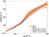Fig. 3. Posterior distribution for EoS. Dark and light yellow bands correspond to the 50% and 90% confidence intervals for the EoS, respectively, obtained including the low- and high-density (LD+HD) filters. Green (magenta) curves indicate the 50% (dashed lines) and 90% (dotted lines) confidence intervals when the crust based on SLy4 (NL3) is used, while blue lines correspond to using the EoS model based on SLy4 until nmatch = 0.16 fm−3 (see text for details).

A complementary way to analyse the impact of the use of a unique crust on the EoS prediction is by looking at the crust–core transition. In Fig. 4, we show the joint distribution of the density and pressure at the crust–core transition, obtained when the polytropes are matched at either 0.16 fm⁻³ (top panels) or at 0.32 fm⁻³ (bottom panels). The prior distributions are shown in the left panels, while the posterior distributions obtained applying the LD+HD filters together with the filters from GW170817 and NICER (LD+HD+LVC+NICER; see Eqs. (51)–(56)) are shown in the right panels. The combined filters considerably reduce the spread in the predictions of the crust–core transition, which is thus relatively well determined. However, the choice of a unique crust completely erases the uncertainties since only a unique value of the crust–core transition point is defined for a given model. This can be seen by comparing the shaded yellow region in the right panels of Fig. 4, with the two symbols representing the crust–core transition for the EoS based on the SLy4 model (red plus symbol) and the NL3 model (red circle) as illustrative examples. Incidentally, the NL3 model is only very marginally compatible with our posterior if the polytrope is matched at 0.16 fm⁻³, as already noticed for the EoS (see Fig. 3), while it is incompatible if the polytrope is matched at 0.32 fm⁻³. This is because in the latter case the stricter EFT filter applied until 0.2 fm⁻³ excludes too stiff models such as NL3.

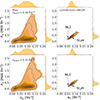Fig. 4. Prior (left panels) and posterior (right panels) distributions for crust–core transition when the piecewise polytrope EoS is matched at nmatch = 0.16 fm−3 (top panels) and at nmatch = 0.32 fm−3 (bottom panels). Dashed black curves represent the 1σ, 2σ, and 3σ confidence levels. Low- and high-density filters together with constraints from GW170817 and NICER (LD+HD+LVC+NICER) are applied. The red cross (circle) indicated by arrows shows the crust–core transition predicted by the EoS based on SLy4 (NL3).

We now discuss the impact of the use of a unique instead of a consistent EoS on more global NS observables. We first show in Fig. 5 the posterior distribution for the radius of a 1.4 M_⊙ NS, R_1.4, as obtained using consistent EoSs (i.e., built as explained in point i), where the matching to a piecewise polytrope is done at n_match = 0.16 fm⁻³; the LD+HD filters are applied (blue shaded area). The use of a unique crust below the crust–core transition (procedure described in point ii.a) does not change the average values of R_1.4 considerably, as can be seen by comparing the blue shaded area with the dash-dotted green (magenta) curves corresponding to the use of the crust EoS based on the SLy4 (NL3) functional. However, when a unique model (in this case, SLy4, dashed blue curve) is applied until n_match (procedure described in point ii.b), although the average value is still not significantly affected, the width of the distribution is reduced, meaning that the use of a unique EoS underestimates the uncertainties.

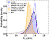Fig. 5. Posterior distribution for radius of a 1.4 M⊙ NS. The blue (orange) shaded area corresponds to the posterior obtained by applying the low- and high-density (LD+HD) filters (combined with the constraints from GW170817 and NICER). The blue and orange dashed curves are obtained by employing a unique EoS based on SLy4 until 0.16 fm−3, while the dash-dotted curves are obtained by employing the crust EoS based on SLy4 (green) and NL3 (magenta) until the crust–core transition. For comparison, the prior is shown by a dotted black line (see text for details).

Additionally, when the filters from GW170817 and NICER are included (orange shaded area), the distribution is shifted to lower radii, as expected since these measurements (and particularly the tidal deformability constraint from GW170817) tend to favour softer EoSs. In this case, the effect of employing a unique EoS until n_match on the average and width of the distribution is reduced, as can be seen by comparing the shaded orange area with the dashed orange curve. This can be understood from the fact that the constraints on the tidal deformability and the radius inferred from GW170817 and NICER observations favour specific values of the radii, thus shifting both distributions towards the same lower radii. For comparison, the prior distribution is shown by a dotted black line; as expected, the prior distribution is much larger, and the applied filters tend to exclude too low (high) values of R_1.4 corresponding to softer (stiffer) EoSs. This was already noticed in Dinh Thi et al. (2021c), where it was pointed out that lower values are filtered by the maximum mass constraint, which would exclude EoSs that are too soft, while higher values corresponding to stiff EoSs are essentially disfavoured by the EFT filter.

To explore the impact of different matching densities, in Fig. 6 we show the comparison among the results on R_1.4 obtained with n_match = 0.16 fm⁻³ (blue curves) and n_match = 0.32 fm⁻³ (red curves). The posterior distributions are obtained including the LD+HD filters (left panel) and the LD+HD filters together with the constraints from GW170817 on the tidal deformability and from NICER (right panel). From both panels in Fig. 6, we can observe that the use of a unique model until n_match underestimates the uncertainties on the radius. This can be understood from the fact that in the latter case the unique (SLy4) model is applied until higher densities, thus constraining the predictions of the observables to those obtained with the chosen EoS. Moreover, matching the polytropes at higher densities noticeably shifts the average value of R_1.4 to lower values and reduces the width of the distribution, even in the priors. This can be due to two effects: first, if n_match = 0.32 fm⁻³, then no phase transition, mimicked by the sudden change of slope that can occur for the polytropic EoS, is allowed (and this is true even for the priors); and, secondly, the EFT filter, which tends to eliminate EoSs that are too stiff and predict higher values of the radius, is applied in a wider density region, thus further constraining the resulting distribution. Incidentally, a similar behaviour can be seen in Fig. 2 of Tews et al. (2018) and Fig. 3 of Tews et al. (2019), although in the latter works a sound-speed model is used instead of a piecewise polytrope. However, when the constraints from the LVC and NICER are applied, the shift in the predicted radius and the difference between the use of a unique EoS instead of a consistent one are decreased because, as already noticed in Fig. 5, these filters tend to favour softer EoSs and thus constrain the radii. The same trend is also observed for the radius of a 1.0 M_⊙ and 2.0 M_⊙ NS, as can be seen from Figs. 7 and 8, respectively.

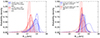Fig. 6. Posterior distribution for radius of a 1.4 M⊙ NS. Left panel: blue (red) shaded area corresponds to posterior obtained by applying the low- and high-density (LD+HD) filters and matching the polytropes at 0.16 fm−3 (0.32 fm−3). The blue and red dashed curves are obtained by employing a unique EoS based on SLy4 until 0.16 fm−3 and 0.32 fm−3, respectively. For comparison, the corresponding priors are shown by dotted lines. Right panel: same as left panel, but the posterior is obtained by applying the low- and high-density filters combined with the constraints from GW170817 and NICER (LD+HD+LVC+NICER; see text for details).

Fig. 7. Same as in Fig. 6, but for radius of a 1.0 M⊙ NS.

Fig. 8. Same as in Fig. 6, but for radius of a 2.0 M⊙ NS.

A similar discussion applies for the tidal deformability of a 1.4 M_⊙ and 2.0 M_⊙ NS, illustrated in Figs. 9 and 10, respectively. Here again, employing a unique EoS model has the effect of slightly shifting the average values and reducing the uncertainties (see left panels of Figs. 9 and 10), and the impact decreases when the filters on the tidal deformability inferred from GW170817 and NICER are applied (see right panels in Figs. 9 and 10). An additional remark is that changing the matching density from n_match = 0.16 fm⁻³ to n_match = 0.32 fm⁻³ considerably decreases the width of the Λ distribution, thus reducing the associated uncertainties. Incidentally, a similar effect can be deduced from Fig. 1 in Tews et al. (2018).

Fig. 9. Same as in Fig. 6, but for tidal deformability of a 1.4 M⊙ NS.

Fig. 10. Same as in Fig. 6, but for tidal deformability of a 2.0 M⊙ NS.

Of particular interest for the NS modelling, and specifically for the glitch modelling, is the NS moment of inertia. Predictions for the moment of inertia, as well as for the crustal thickness, have also been made, for example in Steiner et al. (2015), although in the latter work a simple empirical expression was used to determine the crust–core transition, unlike in this work where it is consistently calculated for each given EoS. In this work, the moment of inertia was calculated following Lattimer & Prakash (2016; see their Eqs. (84)–(85) and Hartle 1967 for the seminal paper on the calculation of the moment of inertia in the slow rotation approximation; see also the discussion in Lattimer & Prakash 2000; Carreau et al. 2019b):

$$\begin{array}{c}\hfill I=\frac{c^2}{G}\frac{w(R)R^3}{6+2w(R)},\end{array}$$(57)

where w(R) is the solution at the star radius R of the differential equation

$$\begin{array}{c}\hfill \frac{\mathrm{d}w}{\mathrm{d}r}=\frac{4\pi G}{c^2}\frac{(\mathcal{E}+P)(4+w)r}{c^2-2G\mathcal{M}/r}-\frac{w}{r}(3+w),\end{array}$$(58)

with the boundary condition w(r = 0) = 0. In the left panel of Fig. 11 we display the posterior distribution for the normalised moment of inertia of a 1.4 M_⊙ NS, I_1.4/(MR²) when the LD+HD filters are applied and the piecewise polytrope is matched at n_match = 0.16 fm⁻³ (blue shaded area). Similarly to what is observed for the radius (see Fig. 5), the use of a unique EoS (dash-dotted curves) slightly shifts the average value; in the case where the unique EoS is employed up to 0.16 fm⁻³ (blue dashed curve), the width of the distribution is considerably reduced. The same trend is seen when the filter from GW170817 and NICER is included in the posterior (orange curves). The impact of the unique EoS model on the uncertainties in the prediction is even larger, as expected, as far as crustal quantities are concerned. This can be seen in the right panel of Fig. 11, showing the fractional moment of inertia of the crust of a 1.4 M_⊙ NS. In this case, the width of the distribution is about an order of magnitude smaller when only one EoS model is considered below the polytrope matching density.

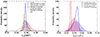Fig. 11. Posterior distributions for moment of inertia of a 1.4 M⊙ NS. Left panel: same as in Fig. 5, but for normalised moment of inertia I1.4/(MR2). Right panel: same as in Fig. 6, but for moment of inertia of crust, Icrust, 1.4/I1.4 for nmatch = 0.16 fm−3 (blue) and nmatch = 0.32 fm−3 (red), when the LD+HD constraints are applied.

The medians and 68% confidence intervals for NS radii, tidal deformabilities, and moment of inertia are summarised for the different treatments of the low-density EoS (crust) in Table 5. The difference in medians with all filters applied between the unique low-density EoS and the full treatment is of the order of a few percent with larger values for the higher matching density. As discussed before, uncertainties are comparable for radii and tidal deformabilities, whereas the unique low-density EoS leads to a considerable reduction for the uncertainties on moments of inertia. Even though the difference in treatment is much smaller than the measurement uncertainty expected for current ground-based GW detectors and their upgrades, it is of the same order as the one expected for third-generation detectors (Chatziioannou 2022; Huxford et al. 2024; Iacovelli et al. 2023). This means that the inference of NS radii and the NS EoS from the data has to handle the treatment of the inhomogeneous part of the EoS in the crust in a consistent way for the upcoming generation of detectors, whereas using a reasonable unique crust, such as the DH(SLY4) model, below its crust–core transition density, should be a good approximation for the current detectors.

As a note of caution, it should be mentioned here that the small difference between the unique crust and the full difference is largely influenced by the filter imposed on the EoS by the chiral-EFT results which strongly constrain the EoS for densities in the crust region. An underestimation of the systematic uncertainties inherent to the chiral-EFT calculations would mean that our results only give a lower limit on the effect of using a unique crust on the results.

Concerning the NS moment of inertia, I, measurements are difficult, and for the moment no precise value exists. There is hope that the Square Kilometer Array (SKA) radio telescope project will be able to obtain it for the double-pulsar PSR J0737−3039A with a level of precision of ≲10% (Watts et al. 2015). Even in the fortunate event that another detected binary NS system provided a more favourable measurement of the moment of inertia, it seems probable, in view of the small differences in the treatment of the crust we obtained here, that using a unique crust model would not have any influence on the inference of NS properties from the moment of inertia, even with the SKA.

4. Conclusions

In this paper, we propose a method to construct consistent and unified crust–core EoSs of cold and beta-equilibrated NSs for application to astrophysical analysis and inference. Starting from a beta-equilibrated relation between the energy density and the baryon number density, together with few nuclear empirical parameters, we show that it is possible to accurately reconstruct a unified and thermodynamically consistent EoS. The associated numerical code CUTER has been tested and validated for use by the astrophysical community, and the first release is currently available. This framework was validated on different nucleonic EoSs (see Sect. 3.1), but is applicable to any beta-equilibrium (high-density) EoSs.

Within a Bayesian analysis and employing a piecewise polytrope at high density to represent the possible existence of non-nucleonic degrees of freedom and phase transitions in the NS core, we assessed the impact of the use of a unique instead of a unified and consistent EoS (crust) model. Our results indicate that the use of a unique EoS model at lower densities underestimates the uncertainties in the prediction of global NS observables, thus highlighting the importance of employing a consistent EoS in inference schemes, which will be particularly important for next-generation detectors.

Acknowledgments

This work has been partially supported by the IN2P3 Master Project NewMAC, the ANR project ‘Gravitational waves from hot neutron stars and properties of ultra-dense matter’ (GW-HNS, ANR-22-CE31-0001-01), the CNRS International Research Project (IRP) ‘Origine des éléments lourds dans l’univers: Astres Compacts et Nucléosynthèse (ACNu)’, the National Science Center, Poland grant 2018/29/B/ST9/02013 and Poland grant 2019/33/B/ST9/00942 and the National Science Foundation grant Number PHY 21-16686. This material is based upon work supported by NSF’s LIGO Laboratory which is a major facility fully funded by the National Science Foundation. The authors gratefully acknowledge the Italian Instituto Nazionale de Fisica Nucleare (INFN), the French Centre National de la Recherche Scientifique (CNRS), and the Netherlands Organization for Scientific Research for the construction and operation of the Virgo detector and the creation and support of the EGO consortium. The authors would like to thank N. Stergioulas and J. Novak for fruitful comments on the code.

References

All Tables

All Figures

Fig. 1. Energy per baryon versus baryon number density for symmetric nuclear matter (SNM; left panels) and for pure neutron matter (PNM; right panels), for the BSk24 (top panels) and the TW99 (bottom panels) models. Dots correspond to the results obtained using the original set of isoscalar and isovector parameters, while dotted blue lines, dash-dotted green lines, and solid red lines correspond to the results from the reconstruction at order 2, 3, and 4, respectively. For comparison, the chiral-EFT calculations of Drischler et al. (2016) are also shown (yellow bands; see text for details).

In the text

Fig. 2. Pressure versus baryon number density (left panels), mass-radius relation (middle panels), and absolute relative error on the radius (right panels) for different models. Crosses and solid black lines (left and middle panel, respectively) correspond to the original EoS, while dotted blue lines, dash-dotted green lines, and solid red lines correspond to the reconstruction at order 2, 3, and 4, respectively (see text for details).

In the text

Fig. 3. Posterior distribution for EoS. Dark and light yellow bands correspond to the 50% and 90% confidence intervals for the EoS, respectively, obtained including the low- and high-density (LD+HD) filters. Green (magenta) curves indicate the 50% (dashed lines) and 90% (dotted lines) confidence intervals when the crust based on SLy4 (NL3) is used, while blue lines correspond to using the EoS model based on SLy4 until nmatch = 0.16 fm−3 (see text for details).

In the text

Fig. 4. Prior (left panels) and posterior (right panels) distributions for crust–core transition when the piecewise polytrope EoS is matched at nmatch = 0.16 fm−3 (top panels) and at nmatch = 0.32 fm−3 (bottom panels). Dashed black curves represent the 1σ, 2σ, and 3σ confidence levels. Low- and high-density filters together with constraints from GW170817 and NICER (LD+HD+LVC+NICER) are applied. The red cross (circle) indicated by arrows shows the crust–core transition predicted by the EoS based on SLy4 (NL3).

In the text

Fig. 5. Posterior distribution for radius of a 1.4 M⊙ NS. The blue (orange) shaded area corresponds to the posterior obtained by applying the low- and high-density (LD+HD) filters (combined with the constraints from GW170817 and NICER). The blue and orange dashed curves are obtained by employing a unique EoS based on SLy4 until 0.16 fm−3, while the dash-dotted curves are obtained by employing the crust EoS based on SLy4 (green) and NL3 (magenta) until the crust–core transition. For comparison, the prior is shown by a dotted black line (see text for details).

In the text

Fig. 6. Posterior distribution for radius of a 1.4 M⊙ NS. Left panel: blue (red) shaded area corresponds to posterior obtained by applying the low- and high-density (LD+HD) filters and matching the polytropes at 0.16 fm−3 (0.32 fm−3). The blue and red dashed curves are obtained by employing a unique EoS based on SLy4 until 0.16 fm−3 and 0.32 fm−3, respectively. For comparison, the corresponding priors are shown by dotted lines. Right panel: same as left panel, but the posterior is obtained by applying the low- and high-density filters combined with the constraints from GW170817 and NICER (LD+HD+LVC+NICER; see text for details).

In the text

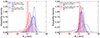	Fig. 7. Same as in Fig. 6, but for radius of a 1.0 M⊙ NS.
In the text

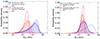	Fig. 8. Same as in Fig. 6, but for radius of a 2.0 M⊙ NS.
In the text

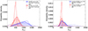	Fig. 9. Same as in Fig. 6, but for tidal deformability of a 1.4 M⊙ NS.
In the text

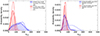	Fig. 10. Same as in Fig. 6, but for tidal deformability of a 2.0 M⊙ NS.
In the text

	Fig. 11. Posterior distributions for moment of inertia of a 1.4 M⊙ NS. Left panel: same as in Fig. 5, but for normalised moment of inertia I1.4/(MR2). Right panel: same as in Fig. 6, but for moment of inertia of crust, Icrust, 1.4/I1.4 for nmatch = 0.16 fm−3 (blue) and nmatch = 0.32 fm−3 (red), when the LD+HD constraints are applied.
In the text

References

- Abbott, B. P., Abbott, R., Abbott, T. D., et al. 2017a, ApJ, 848, L13 [CrossRef] [Google Scholar]
- Abbott, B. P., Abbott, R., Abbott, T. D., et al. 2017b, Phys. Rev. Lett., 119, 161101 [Google Scholar]
- Abbott, B. P., Abbott, R., Abbott, T. D., et al. 2017c, ApJ, 848, L12 [Google Scholar]
- Abbott, B. P., Abbott, R., Abbott, T. D., et al. 2018, Phys. Rev. Lett., 121, 161101 [Google Scholar]
- Abbott, B. P., Abbott, R., Abbott, T. D., et al. 2019, Phys. Rev. X, 9, 011001 [Google Scholar]
- Antoniadis, J., Freire, P. C. C., Wex, N., et al. 2013, Science, 340, 6131 [Google Scholar]
- Baym, G., Pethick, C., & Sutherland, P. 1971, ApJ, 170, 299 [NASA ADS] [CrossRef] [Google Scholar]
- Blaschke, D., & Chamel, N. 2018, in The Physics and Astrophysics of Neutron Stars, eds. L. Rezzolla, P. Pizzochero, D. I. Jones, N. Rea, & I. Vidaña (Cham: Springer International Publishing), Astrophys. Space Sci. Lib., 457, 337 [CrossRef] [Google Scholar]
- Branchesi, M., Maggiore, M., Alonso, D., et al. 2023, J. Cosmol. Astropart. Phys., 2023, 068 [CrossRef] [Google Scholar]
- Burgio, G. F., & Fantina, A. F. 2018, in The Physics and Astrophysics of Neutron Stars, eds. L. Rezzolla, P. Pizzochero, D. I. Jones, N. Rea, & I. Vidaña (Cham: Springer International Publishing), Astrophys. Space Sci. Lib., 457, 255 [NASA ADS] [CrossRef] [Google Scholar]
- Carreau, T., Gulminelli, F., & Margueron, J. 2019a, Eur. Phys. J. A, 55, 188 [CrossRef] [Google Scholar]
- Carreau, T., Gulminelli, F., & Margueron, J. 2019b, Phys. Rev. C, 100, 055803 [NASA ADS] [CrossRef] [Google Scholar]
- Carreau, T., Gulminelli, F., Chamel, N., Fantina, A. F., & Pearson, J. M. 2020, A&A, 635, A84 [NASA ADS] [CrossRef] [EDP Sciences] [Google Scholar]
- Chabanat, E., Bonche, P., Haensel, P., Meyer, J., & Schaeffer, R. 1997, Nucl. Phys. A, 627, 710 [CrossRef] [Google Scholar]
- Chatziioannou, K. 2020, Gen. Relat. Grav., 52, 109 [CrossRef] [Google Scholar]
- Chatziioannou, K. 2022, Phys. Rev. D, 105, 084021 [NASA ADS] [CrossRef] [Google Scholar]
- Christian, J.-E., & Schaffner-Bielich, J. 2020, ApJ, 894, L8 [NASA ADS] [CrossRef] [Google Scholar]
- CompOSE Core Team (Typel, S., et al.) 2022, Eur. Phys. J. A, 58, 221 [NASA ADS] [CrossRef] [Google Scholar]
- Cromartie, H. T., Fonseca, E., Ransom, S. M., et al. 2020, Nat. Astron., 4, 72 [NASA ADS] [CrossRef] [Google Scholar]
- Demorest, P. B., Pennucci, T., Ransom, S. M., Roberts, M. S. E., & Hessels, J. W. T. 2010, Nature, 467, 1081 [Google Scholar]
- Dinh Thi, H., Carreau, T., Fantina, A. F., & Gulminelli, F. 2021a, A&A, 654, A114 [CrossRef] [EDP Sciences] [Google Scholar]
- Dinh Thi, H., Fantina, A. F., & Gulminelli, F. 2021b, Eur. Phys. J. A, 57, 296 [NASA ADS] [CrossRef] [Google Scholar]
- Dinh Thi, H., Mondal, C., & Gulminelli, F. 2021c, Universe, 7, 373 [NASA ADS] [CrossRef] [Google Scholar]
- Douchin, F., & Haensel, P. 2001, A&A, 380, 151 [NASA ADS] [CrossRef] [EDP Sciences] [Google Scholar]
- Drischler, C., Hebeler, K., & Schwenk, A. 2016, Phys. Rev. C, 93, 054314 [Google Scholar]
- Essick, R., Landry, P., & Holz, D. E. 2020a, Phys. Rev. D, 101, 063007 [CrossRef] [Google Scholar]
- Essick, R., Tews, I., Landry, P., Reddy, S., & Holz, D. E. 2020b, Phys. Rev. C, 102, 055803 [NASA ADS] [CrossRef] [Google Scholar]
- Essick, R., Landry, P., Schwenk, A., & Tews, I. 2021, Phys. Rev. C, 104, 065804 [NASA ADS] [CrossRef] [Google Scholar]
- Evans, M., Adhikari, R. X., Afle, C., et al. 2021, arXiv e-prints [arXiv:2109.09882] [Google Scholar]
- Ferreira, M., & Providência, C. 2020, Universe, 6, 220 [NASA ADS] [CrossRef] [Google Scholar]
- Fortin, M., Providência, C., Raduta, A. R., et al. 2016, Phys. Rev. C, 94, 035804 [NASA ADS] [CrossRef] [Google Scholar]
- Goriely, S., Chamel, N., & Pearson, J. M. 2013, Phys. Rev. C, 88, 024308 [NASA ADS] [CrossRef] [Google Scholar]
- Grams, G., Margueron, J., Somasundaram, R., Chamel, N., & Goriely, S. 2022, J. Phys. Conf. Ser., 2340, 012030 [CrossRef] [Google Scholar]
- Greif, S. K., Raaijmakers, G., Hebeler, K., Schwenk, A., & Watts, A. L. 2019, MNRAS, 485, 5363 [NASA ADS] [CrossRef] [Google Scholar]
- Grill, F., Providência, C., & Avancini, S. S. 2012, Phys. Rev. C, 85, 055808 [NASA ADS] [CrossRef] [Google Scholar]
- Grill, F., Pais, H., Providência, C., Vidaña, I., & Avancini, S. S. 2014, Phys. Rev. C, 90, 045803 [NASA ADS] [CrossRef] [Google Scholar]
- Gulminelli, F., & Raduta, A. R. 2015, Phys. Rev. C, 92, 055803 [NASA ADS] [CrossRef] [Google Scholar]
- Haensel, P., Potekhin, A. Y., & Yakovlev, D. G. 2007, Neutron Stars 1: Equation of State and Structure (New York: Springer) [Google Scholar]
- Hartle, J. B. 1967, ApJ, 150, 1005 [NASA ADS] [CrossRef] [Google Scholar]
- Hebeler, K., Lattimer, J. M., Pethick, C. J., & Schwenk, A. 2013, ApJ, 773, 11 [CrossRef] [Google Scholar]
- Hinderer, T. 2008, ApJ, 677, 1216 [NASA ADS] [CrossRef] [Google Scholar]
- Hinderer, T., Lackey, B. D., Lang, R. N., & Read, J. S. 2010, Phys. Rev. D, 81, 123016 [NASA ADS] [CrossRef] [Google Scholar]
- Huang, C., Raaijmakers, G., Watts, A. L., Tolos, L.& Providência, C. 2024, MNRAS, 529, 4650 [CrossRef] [Google Scholar]
- Huxford, R., Kashyap, R., Borhanian, S., et al. 2024, Phys. Rev. D, 109, 103035 [NASA ADS] [CrossRef] [Google Scholar]
- Iacovelli, F., Mancarella, M., Mondal, C., et al. 2023, Phys. Rev. D, 108, 122006 [CrossRef] [Google Scholar]
- Lalazissis, G. A., Nikšić, T., Vretenar, D., & Ring, P. 2005, Phys. Rev. C, 71, 024312 [NASA ADS] [CrossRef] [Google Scholar]
- Landry, P., & Essick, R. 2019, Phys. Rev. D, 99, 084049 [CrossRef] [Google Scholar]
- Lattimer, J. M., & Prakash, M. 2000, Phys. Rep., 333, 121 [CrossRef] [Google Scholar]
- Lattimer, J. M., & Prakash, M. 2016, Phys. Rep., 621, 127 [NASA ADS] [CrossRef] [Google Scholar]
- Lattimer, J. M., Pethick, C. J., Prakash, M., & Haensel, P. 1991, Phys. Rev. Lett., 66, 2701 [NASA ADS] [CrossRef] [Google Scholar]
- Li, B.-A., Ko, C. M., & Bauer, W. 1998, Int. J. Mod. Phys. E, 7, 147 [CrossRef] [Google Scholar]
- Maggiore, M., Van Den Broeck, C., Bartolo, N., et al. 2020, J. Cosmol. Astropart. Phys., 03, 050 [CrossRef] [Google Scholar]
- Margueron, J., Hoffmann Casali, R., & Gulminelli, F. 2018, Phys. Rev. C, 97, 025805 [NASA ADS] [CrossRef] [Google Scholar]
- Maruyama, T., Tatsumi, T., Voskresensky, D. N., Tanigawa, T., & Chiba, S. 2005, Phys. Rev. C, 72, 015802 [NASA ADS] [CrossRef] [Google Scholar]
- Miller, M. C., Lamb, F. K., Dittmann, A. J., et al. 2019, ApJ, 887, L24 [Google Scholar]
- Miller, M. C., Lamb, F. K., Dittmann, A. J., et al. 2021, ApJ, 918, L28 [NASA ADS] [CrossRef] [Google Scholar]
- Mondal, C., & Gulminelli, F. 2022, Phys. Rev. D, 105, 083016 [NASA ADS] [CrossRef] [Google Scholar]
- Newton, W. G., Gearheart, M., & Li, B.-A. 2013, ApJS, 204, 9 [NASA ADS] [CrossRef] [Google Scholar]
- Oertel, M., Hempel, M., Klähn, T., & Typel, S. 2017, Rev. Mod. Phys., 89, 015007 [Google Scholar]
- Oppenheimer, J. R., & Volkoff, G. M. 1939, Phys. Rev., 55, 374 [NASA ADS] [CrossRef] [Google Scholar]
- Pearson, J. M., Chamel, N., Potekhin, A. Y., et al. 2018, MNRAS, 481, 2994 [NASA ADS] [Google Scholar]
- Pearson, J. M., Chamel, N., Potekhin, A. Y., et al. 2019, MNRAS, 486, 768 [NASA ADS] [CrossRef] [Google Scholar]
- Raaijmakers, G., Riley, T. E., Watts, A. L., et al. 2019, ApJ, 887, L22 [NASA ADS] [CrossRef] [Google Scholar]
- Raduta, A. R. 2022, Eur. Phys. J. A, 58, 115 [NASA ADS] [CrossRef] [Google Scholar]
- Raithel, C. A., & Most, E. R. 2023a, Phys. Rev. Lett., 130, 201403 [NASA ADS] [CrossRef] [Google Scholar]
- Raithel, C. A., & Most, E. R. 2023b, Phys. Rev. D, 108, 023010 [NASA ADS] [CrossRef] [Google Scholar]
- Ravenhall, D. G., Pethick, C. J., & Lattimer, J. M. 1983, Nucl. Phys. A, 407, 571 [NASA ADS] [CrossRef] [Google Scholar]
- Read, J. S., Lackey, B. D., Owen, B. J., & Friedman, J. L. 2009, Phys. Rev. D, 79, 124032 [NASA ADS] [CrossRef] [Google Scholar]
- Riley, T. E., Watts, A. L., Bogdanov, S., et al. 2019, ApJ, 887, L21 [Google Scholar]
- Riley, T. E., Watts, A. L., Ray, P. S., et al. 2021, ApJ, 918, L27 [CrossRef] [Google Scholar]
- Salmi, T., Vinciguerra, S., Choudhury, D., et al. 2022, ApJ, 941, 150 [CrossRef] [Google Scholar]
- Steiner, A. W., Gandolfi, S., Fattoyev, F. J., & Newton, W. G. 2015, Phys. Rev. C, 91, 015804 [NASA ADS] [CrossRef] [Google Scholar]
- Suleiman, L., Fortin, M., Zdunik, J. L., & Haensel, P. 2021, Phys. Rev. C, 104, 015801 [NASA ADS] [CrossRef] [Google Scholar]
- Suleiman, L., Fortin, M., & Zdunik, J. L. 2022, Phys. Rev. C, 106, 035805 [NASA ADS] [CrossRef] [Google Scholar]
- Tang, S.-P., Jiang, J.-L., Gao, W.-H., Fan, Y.-Z., & Wei, D.-M. 2021, Phys. Rev. D, 103, 063026 [NASA ADS] [CrossRef] [Google Scholar]
- Tews, I., Margueron, J., & Reddy, S. 2018, Phys. Rev. C, 98, 045804 [NASA ADS] [CrossRef] [Google Scholar]
- Tews, I., Margueron, J., & Reddy, S. 2019, Eur. Phys. J. A, 55, 97 [CrossRef] [Google Scholar]
- Tolman, R. C. 1939, Phys. Rev., 55, 364 [NASA ADS] [CrossRef] [Google Scholar]
- Typel, S., & Wolter, H. H. 1999, Nucl. Phys. A, 656, 331 [Google Scholar]
- Typel, S., Oertel, M., & Klähn, T. 2015, Phys. Part. Nucl., 46, 633 [CrossRef] [Google Scholar]
- Wang, M., Huang, W. J., Kondev, F. G., Audi, G., & Naimi, S. 2021, Chin. Phys. C, 45, 030003 [CrossRef] [Google Scholar]
- Watts, A., Xu, R., Espinoza, C., et al. 2015, PoS, AASKA14, 043 [NASA ADS] [Google Scholar]
- Weiss, A., Hillebrandt, W., Thomas, H. C., & Ritter, H. 2004, Cox and Giuli’s Principles of Stellar Structure (Cambridge: Cambridge Scientific Publishers Ltd.) [Google Scholar]
All Tables
Baryon number density points nB, j (in fm−3) for the EoS reconstruction according to different orders N.
Nuclear empirical parameters for the BSk24, SLy4, DDME2, and TW99 models used in this work.
Crust–core transition (baryon number density ncc and pressure Pcc) for the EoSs based on the BSk24, SLy4, DDME2, and TW99 models.
Medians and 68% confidence intervals of NS radii, dimensionless tidal deformabilities, moment of inertia, and crustal moment of inertia for a M = 1.4 M⊙ NS.