| Issue |
A&A
Volume 694, February 2025
|
|
|---|---|---|
| Article Number | A290 | |
| Number of page(s) | 15 | |
| Section | Interstellar and circumstellar matter | |
| DOI | https://doi.org/10.1051/0004-6361/202452496 | |
| Published online | 20 February 2025 | |
The centimeter emission from planet-forming disks in Taurus
1
INAF – Istituto di Radioastronomia,
Via Gobetti 101,
40129
Bologna,
Italy
2
Max-Planck-Institut für Astronomie,
Königstuhl 17,
69117
Heidelberg,
Germany
3
Instituto de Radioastronomía y Astrofísica (IRyA-UNAM),
Morelia,
Michoacán
58089,
Mexico
4
European Southern Observatory,
Karl-Schwarzschild-Strasse 2,
85748
Garching,
Germany
5
Dipartimento di Fisica e Astronomia Augusto Righi, Università di Bologna,
Viale Berti Pichat 6/2,
Bologna,
Italy
6
Dipartimento di Fisica, Università degli Studi di Milano,
Via Celoria 16,
20133
Milano,
Italy
7
Departamento de Astronomía, Universidad de Chile,
Camino El Observatorio 1515, Las Condes,
Santiago,
Chile
8
Department of Physics and Astronomy, California State University Northridge,
18111 Nordhoff Street,
Northridge,
CA
91330,
USA
9
Lunar and Planetary Laboratory, University of Arizona,
Tucson,
AZ
85721,
USA
10
Institute of Astronomy, University of Cambridge,
Madingley Road,
Cambridge
CB3 0HA,
UK
11
Kavli Institute for Astronomy and Astrophysics, Peking University,
Yiheyuan 5, Haidian Qu,
100871
Beijing,
China
12
Department of Astronomy, Peking University,
Yiheyuan 5, Haidian Qu,
100871
Beijing,
China
13
Department of Physics and Astronomy, Rice University,
6100 Main Street, MS-108,
Houston,
TX
77005,
USA
14
Leiden Observatory, Leiden University,
PO Box 9513,
2300 RA
Leiden,
The Netherlands
15
INAF, Osservatorio Astrofisico di Arcetri,
Largo Enrico Fermi 5,
50125
Firenze,
Italy
★ Corresponding author; This email address is being protected from spambots. You need JavaScript enabled to view it.
Received:
4
October
2024
Accepted:
16
January
2025
Abstract
The last decade has witnessed remarkable advances in the characterization of the (sub-)millimeter emission from planet-forming disks. Conversely, the study of (sub-)centimeter emission has made more limited progress, to the point that only a few exceptional disk-bearing objects have been characterized in the centimeter regime. This work takes a broad view of the centimeter emission from a large sample with Karl G. Jansky Very Large Array (VLA) observations that is selected from previous Atacama Large (sub-)Millimeter Array (ALMA) surveys of more representative disks in brightness and extent. We report on the detection and characterization of flux at centimeter wavelengths from 21 sources in the Taurus star-forming region. Complemented by literature and archival data, the entire photometry from 0.85 mm to 6 cm is fit by a two-component model that determines the ubiquitous presence of free-free emission entangled with the dust emission. The flux density of the free-free emission is found to scale with the accretion rate but is independent of the outer-disk morphology depicted by ALMA. The dust emission at 2 cm is still appreciable and offers the possibility to extract an unprecedented large set of dust spectral indices in the centimeter regime. A pronounced change between the median millimeter indices (2.3) and centimeter indices (2.8) suggests that a large portion of the disk emission is optically thick up to 3 mm. The comparison of both indices and fluxes with the ALMA disk extent indicates that this portion can be as large as 40 au and suggests that the grain population within this disk region that emits the observed centimeter emission is similar in disks with different sizes and morphologies. All these results await confirmation and dedicated dust modeling once facilities such as next generation VLA (ngVLA) or Square Kilometre Array (SKA)-mid are able to resolve the centimeter emission from planet-forming disks and disentangle the various components.
Key words: techniques: interferometric / protoplanetary disks / stars: pre-main sequence
NASA Hubble Fellowship Program Sagan Fellow.
© The Authors 2025
 Open Access article, published by EDP Sciences, under the terms of the Creative Commons Attribution License (https://creativecommons.org/licenses/by/4.0), which permits unrestricted use, distribution, and reproduction in any medium, provided the original work is properly cited.
This article is published in open access under the Subscribe to Open model. This email address is being protected from spambots. You need JavaScript enabled to view it. to support open access publication.
1 Introduction
Much progress has been made in the characterization of planetforming disks over the last decade. The advent of the Atacama Large (sub-)Millimeter Array (ALMA; see, e.g., ALMA Partnership 2015) and of the extreme adaptive optics facilities (see review by Benisty et al. 2023) has enabled the imaging of the circumstellar disks around Class II objects (Lada 1987) with high resolution (less than 0.1″) and high contrast (of the order of 10−5 ). One of the benefits of this type of observation is the possibility to detect and resolve the bulk population of planet-forming disks, namely those disks with an extent of a few tens of astronomical units (0.2″–0.3″ at the distance of the closest star-forming regions). The reason why the community aimed efforts at the characterization of the inner few tens of au is twofold. On the one hand, planet formation via core accretion is favored in this disk region (e.g., Pollack et al. 1996). On the other hand, a less biased view of planet-forming disks (switching from the characterization of extremely large disks to that of ordinary objects) is necessary to bridge the fields of planet formation and exoplanets (see, e.g., Mulders et al. 2021; van der Marel & Mulders 2021; Miotello et al. 2023).
The main finding on the bright and extended planet-forming disks that have been surveyed by sub-millimeter and nearinfrared (near-IR) high-resolution images is the high occurrence of disk substructures (see, e.g., Andrews et al. 2018; Garufi et al. 2018). Different explanations have been put forward to explain the origin of these substructures (see review by Bae et al. 2023), such as the interaction with planets (see, e.g., Kley 1999; Crida et al. 2006) or the presence of instabilities (see review by Lesur et al. 2023). The first type of substructure to be studied was disk cavities (pioneering images by, e.g., Dutrey et al. 1994; Fukagawa et al. 2006; Brown et al. 2009; Andrews et al. 2011). Cavities are revealed as a large inner portion (a few to several tens of au) of the disk with a diminished dust emission. Cavity-hosting disks (often referred to as transition disks) are, however, a very peculiar path (or stage) of the disk evolution, and this type of disks only represents 10% or less of the total disk population (see review by van der Marel 2023 and references therein). In view of this, much effort has been made to improve our understanding of full disks (as opposed to transition disks) and the morphology of other possible substructures such as rings and gaps.
When observed in near-IR scattered light, full disks appear much fainter than cavity-hosting disks because the inner portion of the disk at (sub-)au scales casts a shadow on the outer, resolvable disk (Dullemond & Dominik 2004; Garufi et al. 2017, 2022). When observed by ALMA, the inner region of full disks tends to appear bright and smooth (see, e.g., Andrews et al. 2018; Long et al. 2019). The correlation between the disk size and luminosity from millimeter images suggests that the emission from a significant portion of the disk may be optically thick (Tripathi et al. 2017; Tazzari et al. 2021a). Also, dust scattering can lower the disk emission and decrease the measured optical depth of possibly optically thick emission (Birnstiel et al. 2018; Zhu et al. 2019; Sierra & Lizano 2020). Optically thick emission can also be constrained from the occultation of background material (such as a back-side outflow cavity; see Garufi et al. 2020) or from the CO brightness decrease in proximity of continuum rings (Isella et al. 2018; Guzmán et al. 2018). The possibility that some disk emission is optically thick poses severe limitations to the study of the dust-grain properties since a high optical depth can conceal the actual dust density and alter the measured spectral indices in a similar manner to the growth of particles to millimeter sizes.
The (sub-)centimeter emission from disks (frequencies ν ∼ 10–100 GHz) is therefore an essential tool to probe dust densities and grain properties because the optical depth is sufficiently low, while the disk emission is still strong enough to be detected in a reasonable amount of telescope time. While the current generation of radio interferometers does not offer the resolving power of ALMA, these may still provide pivotal constraints on the dust properties through unresolved images, or moderately resolved images at the higher frequencies for large and bright disks. The Karl G. Jansky Very Large Array (VLA) and the Australia Telescope Compact Array (ATCA) have produced promising results in this direction focusing on bright disks such as those of LkCa15 (Isella et al. 2014), GM Aur (Macías et al. 2016, 2018), MWC758 (Marino et al. 2015; Casassus et al. 2019), HD 169142 (Macías et al. 2017), HL Tau (Carrasco-González et al. 2016, 2019), HD 142527 (Casassus et al. 2015), DM Tau (Liu et al. 2024), and HD 163296 (Guidi et al. 2022); as well as on 15 disks with known large cavities (Norfolk et al. 2021).
In this study, we moved the focus from the (sub-)centimeter emission of extraordinary, individual objects to a large sample of ordinary disks imaged with VLA in the Taurus star-forming region. The Taurus-Auriga complex is one of the closest starforming regions (Galli et al. 2018) hosting a few hundred low-mass stars (Esplin & Luhman 2019) at diverse evolutionary stages (Kenyon et al. 2008). With more than 60 members with high-resolution images of the disk available, it is among the most studied star-forming regions. The ALMA and near-IR surveys of Taurus from the literature are extensively described in Sect. 2, along with the new VLA dataset. Then, in Sect. 3 we analyze the VLA observations, focusing on the unresolved information. At centimeter wavelengths, non-dust emission (e.g., free-free and synchrotron emission) plays an important role. Therefore, the images are modeled to disentangle the photometry from the dust emission and that from non-dust emission (Sects. 3.1 and 3.2). The non-dust emission is analyzed in Sect. 3.3, while the dust emission is covered in Sects. 3.4 and 3.5. Finally, we discuss our results and conclude in Sects. 4 and 5.
2 Sample and observing setup
The sample analyzed in this work consists of 21 sources in Taurus with VLA observations available. In this section, we describe the stellar and disk properties known from the literature (Sect. 2.1) and present the new (sub-)centimeter observations from VLA (Sect. 2.2) as well as some complementary observations from CARMA (Sect. 2.3).
2.1 Target properties
All the sources in this work are part of the ALMA survey described by Long et al. (2018, 2019). Their original sample was compiled from the whole known census of Taurus, only excluding stars of types later than M3 and close-binary-system types and highly extincted sources. In addition, they avoided all disks with existing high-resolution ALMA images at that time. This was the main bias of the selection as it excludes all well-studied (and often extraordinarily bright and extended) disks such as those of AB Aur, GM Aur, and GG Tau.
Within their original sample, Long et al. (2019) revealed 12 disks with evident dust gaps and rings (hereafter substructured disks) and 20 disks with no resolvable substructures. The substructured disks have an effective dust radius with 95% flux enclosed larger than 50 au, while the other disks are all smaller than that (motivating the definition of compact disks hereafter). The inner part of substructured disks show similar brightness properties to the compact disks, making the existence of substructures beyond ∼50 au the key difference between the two categories. Our sample comprises ten substructured disks and 11 compact disks, as shown in Table 1 along with their effective radius1.
Of the 21 sources analyzed in this work, 18 have also been observed in near-IR scattered light with VLT/SPHERE (Garufi et al. 2024). All these disks appear relatively faint in scattered light. This reflects the aforementioned absence from the sample by Long et al. (2019) of extraordinarily large disks with large cavities that are typically bright in scattered light (see Garufi et al. 2017). However, three of the 18 targets observed with SPHERE (DO, DR, and HP Tau) show evidence of ambient material (envelopes, outflows, streamers). This material is mostly composed of interstellar gas and µm-sized dust grains that escape the continuum surveys by ALMA.
The stellar properties of the sample are also listed in Table 1. Most of the sources are sub-solar-mass stars, with the only exceptions being HP Tau, HQ Tau, and MWC 480. The ages are typically in the 1–3 Myr interval, as expected for the Taurus star-forming region (see Garufi et al. 2024 for details). The mass accretion rates vary substantially within the sample spanning from 2.5 ⋅ 10−8 M⊙ yr−1 (DL Tau) to 2.5 ⋅ 10−11 M⊙ yr−1 (HP Tau).
Main properties of literature sample.
2.2 VLA observations and data reduction
We made use of VLA observations of the Taurus star-forming region in the Q band (bandwidth: 39–47 GHz, λc=7 mm), Ka band (29–37 GHz, λc = 1 cm), K band (18–26 GHz, λc = 1.3 cm), Ku band (12–18 GHz, λc = 2 cm), and C band (4– 8 GHz, λc = 6 cm). All observations are from projects 20A-373 (PI: M. Tazzari) and 21B-267 (PI: C. Carrasco-Gonzalez). All sources are observed in the Ku band, and 19 of them are also in the Ka band. Only nine sources are observed in the Q and K bands, and ten sources are observed in the C band. The observations in the Q, Ka, and K bands were taken in B array configuration, resulting in typical beam sizes of 0.15″, 0.25″, and 0.35″, respectively, while those in the Ku and C bands were taken in the C configuration, yielding beam sizes of approximately 1.4″ and 3″, respectively. The typical RMSs of the observations are on the order of a few µJy. The details of each individual dataset are given in Table A.2.
Data were first calibrated by the VLA pipeline. Secondly, phase self-calibration was performed on all clear detections using the software CASA, version 6.4. Each dataset was spectrally averaged and shifted to a common center across multiple wavebands. The cleaning procedure was performed by employing a Briggs weighting of 0.5 and making sure that even background sources at the edge of the field of view (on a scale of several arcminutes) were properly masked. The lack of this operation would in fact result in a dramatic increase for the flux of the central source after the first round of self-calibration (up to 4–5 times the initial value). Instead, the images obtained after one round of self-calibration performed with the largest possible solution interval and with a minimum S/N of 2 for each polarization independently and combining across scans exhibit a central flux that is typically 10% higher than the original value, with only a few cases reaching up to 20%. Further rounds of selfcalibration with shorter solution intervals or combining across spectral windows were always unnecessary to recover any additional flux. We find no correlation between the amount of flux recovered and the initial brightness of the source.
2.3 CARMA observations and data reduction
We also made use of unpublished CARMA data of seven sources from the CARMA data archive2 that will be described in depth by Blair et al. (in prep.). The inclusion of these data is motivated by the poor photometry available from the literature at 3 mm (see Sect. 3.2), with only 13 of our 21 sources having published 3 mm photometry.
The CARMA observations in question consist of 100– 113 GHz images of the entire sample (except CIDA 9, UZ Tau, and V409 Tau) that were taken between October 2009 and December 2012. The images were acquired using the sub-array with 15 antennas in C, D, and E configurations resulting in a minimum angular resolution of 1.8″. The data were calibrated and optimized with the MIRIAD software as is described in detail by Blair et al. (in prep.).
3 Results
In this section, we analyze the new VLA observations. First, an overview of the VLA images is given in Sect. 3.1. Then, the spectral energy distributions (SEDs) of the sample are modeled with two power laws (Sect. 3.2), and the results from non-dust emission are presented in Sect. 3.3. After that, the dust emission is analyzed in Sects. 3.4 and 3.5.
3.1 Overview of the VLA images
All sources are detected in the Q, Ka, K, and Ku band when the respective data are available. Instead, only two sources (BP Tau and HQ Tau) are detected in the C band, with the latter being a very marginal detection. The signal in all Ku-band images is unresolved, while it is marginally resolved in some Ka-band images and clearly resolved in most Q-band images. An investigation of the resolved component of the Q- and Ka-band images is deferred to a forthcoming study. In this work, we focused on the integrated flux at the Q band through the C band, putting particular emphasis on the Ku-band data (2 cm) on which very few studies have been carried out in the past. All images in the Ku band are shown in Fig. A.2.
The total flux associated with each source and waveband was measured through a Gaussian fit performed with the CASA task IMFIT. The measured fluxes are reported in Table A.2. These typically span from a few milliJansky at the higher frequencies to a few tens of milliJansky at the lower frequencies. Two datasets represent a notable exception: the Ku-band flux of HP Tau (7 mJy, that is, two orders of magnitude higher than the other sources) and the K-band flux of DQ Tau (31 mJy). These two measurements are discussed in Sect. 4.3.
3.2 Spectral energy distribution
The VLA and CARMA photometry of each source was then placed in a SED together with the photometry at 850 µm from SCUBA (Andrews & Williams 2005), at 1.06 mm from CSO (Beckwith & Sargent 1991), at 1.33 mm from ALMA (Long et al. 2019), and at 2.7–3.5 mm from the IRAM Plateau de Bure Interferometer (Dutrey et al. 1996; Ricci et al. 2010).
A first visual inspection of the SEDs revealed a clear flattening of the trend for the photometry at wavelengths longer than 1 cm. This suggests the presence of an extra radio emission component such as free-free emission from jets (e.g., Anglada et al. 2018) and photo-evaporating wind (Pascucci et al. 2012) or gyrosynchrotron radiation from magnetically induced stellar flares (Dulk & Marsh 1982). A useful tool to disentangle free-free and gyro-synchrotron emission is the spectral slope of the associated SED, with the former emission producing positive slopes with the frequency (Panagia & Felli 1975; Reynolds 1986) and the latter producing negative slopes from ∼5 GHz on (Bastian et al. 1998); these are positive trends with a wavelength up to ∼5 cm. The systematic nondetection of any flux in our C-band images (at 6 cm) and the lower fluxes recorded in the Ku (2 cm) compared to the Ka (1 cm) intuitively advocate for a free-free emission being responsible for the extra radio emission.
To quantify the contribution from the ionized gas in our sources (free-free emission or gyro-synchrothron emission), each SED was therefore fit with a simple model consisting of the sum of two power laws, each of them representing the behavior with the observed frequency of an emission mechanism:
 (1)
(1)
where  is the flux density contribution at a wavelength of 2 cm (frequency of 15 GHz),
  is the flux density contribution at a wavelength of 1.3 mm (frequency of 225 GHz), and αgas and αdust are the spectral indices of the ionized gas (free- free or synchrotron) and dust contributions, respectively. For the fitting, we imposed some constraints, namely that
  and
and  cannot be larger than the measured total flux densities at 2 cm and 1.3 mm, respectively; that αgas should be within the range [−1.0, 2.0]; and that αdust should be within the [2.0, 4.0] range. The space parameter was explored using a Markov chain Monte Carlo (MCMC) algorithm with 20 000 iterations and 40 walkers. The initial values of each walker is set randomly (with a flat probability) within the allowed range for each parameter. For the final statistics, we only considered the last 10 000 iterations. The SED fits are shown in Figs. 1 (one illustrative case) and A.3 (all cases).
The illustrative SED of DR Tau shown in Fig. 1 reveals that some non-dust emission is detectable and starts to dominate over the dust emission at wavelengths longer than 1 cm. For this specific case, our model determines a non-dust emission at 2 cm of  mJy and a spectral slope αgas of
  . The αgas constrained for the sample spans from 0.3 to 1.1 (with 15 of 21 being between 0.5 and 1.0). Since these are the slopes expected from free-free emission (Panagia & Felli 1975; Reynolds 1986), hereafter we refer to the ionized gas emission as free-free emission. All fluxes and slopes constrained by our model are listed in Table A.1.
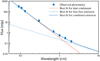 |
Fig. 1 Illustrative SED. The observed photometry of DR Tau is fit by two power laws for the dust continuum and the free-free emission. All derived slopes and all SEDs are shown in Table A.1 and Fig. A.3, respectively. |
3.3 Free-free emission
All SEDs are well fit by our model from Sect. 3.2, supporting a view where the extra emission at radio wavelengths is free-free emission. Overall, we determined the presence of some free-free emission at 2 cm in all sources. In absolute terms, our measured free-free emission spans from the barely detectable value of 0.02 mJy (CIDA 9 and V409 Tau) to the very large value of the Herbig AeBe star MWC 480 (0.24 mJy) and that of the spectroscopic binary DQ Tau (0.26 mJy). The latter source is the only case where the SED fitting presents some criticalities, which are discussed in Appendix A. Furthermore, the peculiar case of HP Tau with very poor photometry (see Fig. A.3) is not treated by our model. For this source, the photometric value is high enough (7 mJy) to assure that any dust contribution is negligible (since a simple fit to the available ALMA photometry results in a dust contribution at 2 cm of less than 0.1 mJy).
In relative terms, our model constrains that the free-free emission contributes on average 65% of the total flux at 2 cm. The scatter of this fraction across the sample is very narrow (σ = 8%) meaning that, for Class II objects at 2 cm, an equal partition between free-free and dust emission can be coarsely assumed. In contrast, the contribution to the total flux at 1 cm by the free-free emission spans from 10% (DL Tau) to 75% (GK Tau), with an average of 35%, meaning that each case should be evaluated individually. At 3 mm, the distribution of this fraction is again quite narrow around a median value of 5%, while it is less than 2% in most cases at 1.3 mm (see histogram in Fig. A.1).
The origin of the free-free emission from a relatively large sample can be investigated from its relation with other observable quantities. First, our estimates of the free-free emission scaled at an equal distance have a loose relation with the stellar mass of Table 1 (Pearson coefficient r = 0.51 ± 0.19), although the narrow interval of stellar masses involved (more than half of the sample between 0.4 and 0.6 M⊙) may conceal any tighter connection. Inspired by the correlation between the accretion rate and the free-free emission that was recently reported by Rota et al. (2024) for transition disks, we relate these two quantities in Fig. 2. Our estimates of the free-free emission come with relatively large error bars owing to the unresolved nature of the 2cm emission and the consequent need for the model described in Sect. 3.2. Nonetheless, a clear correlation (with r = 0.66 ± 0.17) between this emission and the mass accretion from Table 1 is visible from Fig. 2. Low accretors (in the framework of this sample, sources with less than 10−8 M⊙ yr−1 ) show a free-free emission at 2 cm and at 140 pc of less than 0.1 mJy, while the opposite is shown by high accretors. The correlation holds if we instead consider the total flux observed at 2 cm (without employing any model to determine the free-free emission). This is not surprising if we consider the aforementioned fraction of free-free over total flux at 2 cm, which is rather constant across the sample.
Interestingly, the trend of Fig. 2 does not reveal any segregation between the substructured disks and the compact disks by Long et al. (2019, see our Sect. 2.1) with both categories being equally distributed across the observed interval of values (resulting in a Pearson r between free-free emission and disk extent from Table 1 as low as 0.06). This would intuitively indicate that the origin of the correlation is completely independent of the presence of disk substructures more than 50 au from the star.
Rota et al. (2024) concluded that the free-free emission determined for their sample is related to the ionized jet and that the observed trend reflects the connection between the outflow and accretion activities. Further analyses on the free-free emission of our sample and an in-depth discussion of the implication of Fig. 2 are given in a forthcoming publication by Rota et al. (in prep.).
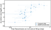 |
Fig. 2 Free-free emission versus mass accretion rate. The free-free emission at 2 cm constrained by our model (see Sect. 3.2) for the entire sample is scaled to 140 pc and compared with the mass-accretion rates shown in Table 1. Despite large errors, a correlation between both quantities is clearly seen across several orders of magnitude. Nonetheless, the distribution of compact disks against substructured disks appears random. HP Tau (with a free-free emission at 140 pc of approximately 10 mJy and an accretion rate of 2.5 ⋅ 10−11 M⊙ yr−1) clearly falls out of the correlation and is not shown in order to provide a better view of the plot. |
3.4 Dust spectral indices
The slope of the millimeter SED α defined as
 (2)
(2)
is a useful diagnostic of the dust properties since, for optically thin emission in the Rayleigh-Jeans regime, it relates to the dust opacity spectral index β through β = α − 2. However, an important restriction on this conversion is imposed by the aforementioned optically thick nature of a significant extent of disks up to 3 mm (e.g., Ribas et al. 2020; Sierra & Lizano 2020; Tazzari et al. 2021a; Xin et al. 2023). Therefore, the measurement of α at (sub-)centimeter wavelengths represents a viable tool to alleviate this problem since we can assume that this emission is genuinely optically thin.
The 0.89–1.33 mm spectral index α1mm extracted from Andrews et al. (2013) for our sources is on average 2.4 (with a σ = 0.3). Rather lower values (2.0) are found from the recent SMA survey of Taurus by Chung et al. (2024), although the difference is more marginal within the intersecting sample (2.3 vs. 2.1). Similarly, the 1.33–3 mm index α3mm of our sample from the photometry introduced in Sect. 3.2 is on average 2.3 (with a σ = 0.4). A possible interpretation of integrated values so close to 2 is that the optically thick portion of the disk at these wavelengths is lowering the actual averaged α of the disk. We therefore made use of our centimeter photometry to extend these indices to longer wavelengths.
A first hint to higher values of α comes from the αdust values of our model (see Sect. 3.2) shown in Table A.1. Their average is 2.7, with a low dispersion (σ = 0.2). Thus, we extracted the individual indices from the observed 1-cm and 2-cm photometry after removing the free-free contribution described in Sect. 3.3. The same procedure was applied to the millimeter photometry even though the contribution from the free-free in that regime is on average only 5% at most. In line with the αdust from the model, the index between 3 mm and 1 cm α1cm turned out to be 2.8±0.3, which is substantially higher than the aforementioned 2.4±0.3 from α1 mm.
Finally, we measured the index at even longer wavelengths, exploiting the 1-cm and 2-cm photometry. In this regime, the impact of the free-free emission is significant (approximately 65%; see Sect. 3.3), and the error bars on the index are larger since the flux is detected with lower significance. Therefore these indices, in the absence of any resolved image, are inevitably rather uncertain. In fact, our measured indices α2cm between the 1-cm and 2-cm photometry turned out to be much more varied than all other indices. In particular, six sources have an error larger than 1.0, which makes the measured index meaningless. Excluding these sources from the overall measurement, the average (2.7±0.4) is very similar to that of the α1cm. Figure 3 summarizes these findings manifesting that the averaged spectral indices have a pronounced change between the (sub-)millimeter and the (sub-)centimeter wavelengths, while they remain stable within the two regimes.
A further step to evaluate the measured spectral indices is the comparison with the disk extent measured from ALMA (Long et al. 2019, see Table 1). For this exercise, we used the α between 0.89 mm and 3 mm, since the intermediate indices within this interval are very similar (see Fig. 3), and between 3 mm and 1 cm, since these have smaller errors than those between 1 cm and 2 cm. As is clear from Fig. 4, the five smaller disks in the sample (r < 40 au) exhibit a millimeter index that is consistent with 2.0, while larger disks have a significantly larger value (on average 2.4). A similar trend of larger indices for larger disk extents is found by Tazzari et al. (2021a) for α at the same wavelengths and by Chung et al. (2024) for α between 0.85 and 1.3 mm. Conversely, our measured α between 3 mm and 1 cm is significantly larger for smaller disks, while it is only slightly larger for bigger disks. This trend results in an index distribution with the disk extent that is nearly constant. As discussed in Sect. 4.1, the behavior described in this section is consistent with a view where the inner few tens of au of disks are optically thick up to ∼3 mm, while the optical depth severely decreases at longer wavelengths. It also highlights that the sub-centimeter indices from the optically thin emission of substructured and compact disks are not significantly different (see the flat trend in Fig. 4).
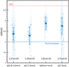 |
Fig. 3 Millimeter and centimeter dust spectral indices. The individual α at four different spectral ranges are shown in semi-transparency. These are obtained by removing the free-free emission from our photometry and comparing with literature values (see text). The big foreground symbols are the average values for the entire sample. The error bars of the individual sources are inherited from the uncertainty on the photometry, while those of the averages are the dispersion of the relative sample. The red line indicates the spectral index of the interstellar dust grains in the millimeter index, while the blue line shows the expected index from optically thick emission. |
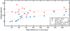 |
Fig. 4 Dust spectral indices versus disk extent. All available α of our sample obtained after removing the free-free emission are compared with the disk extent from the ALMA continuum emission at 1.3 mm listed in Table 1. The best fits to the data are shown as dashed lines. A small offset in extent is given to some datapoints so that indices at the same radius, when available, are from the same object. |
3.5 Dust-integrated emission
The dust emission at millimeter and centimeter wavelengths also offers the possibility to probe the mass budget in solids. For optically thin emission in the Rayleigh-Jeans regime, the integrated flux is in fact directly converted into dust mass under some assumptions on the dust opacity (discussed in Sect. 4.2). Here, we compare the millimeter and centimeter fluxes of substructured and compact disks (Sect. 2.1) of the sample, leaving aside the conversion to the actual mass.
As is clear from Fig. 5, the average total flux of substructured disks3 normalized at an equal distance is 73% larger than that of compact disks. However, this value decreases to 54% at 3 mm and then remains constant up to 2 cm. It is thus tempting to conclude that we are seeing another manifestation of the optically thick nature of the 1.3-mm emission. In fact, the mass of compact disks would be more under-estimated than that of extended disks because they have a larger portion of optically thick emission (see also Sanchez et al. 2024).
To test this interpretation, we repeated the same exercise with the highly resolved flux from the 1.3-mm ALMA images. As expected, diminishing the aperture over which the total flux is integrated results in lowering the difference between substructured and compact disks. In particular, Fig. 4 had suggested that the inner 40 au of disks could be heavily optically thick. Interestingly, when we consider an aperture of 40 au (which is still larger than the extent of most compact disks), substructured disks are only 59% brighter than compact disks (see red points in Fig. 5); that is, they are much closer to the value found on the total flux at longer wavelengths. This suggests that the compact disks of this sample have 50%–60% intrinsically lower masses than the extended disks and that the 73% recorded at 1.3 mm is the effect of the optical depth being relatively more significant in compact disks. This does indicate a net loss of 1.3-mm flux in these disks, but it does qualitatively suggest that is very high, even for extended disks, since an average of as much as 65% of the flux from this type of disk in our sample is from the inner 40 au.
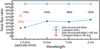 |
Fig. 5 Total flux ratio between substructured and compact disks at different wavelengths. The average dust-integrated flux at the same distance of compact disks from 1.3-mm, 3-mm, 1-cm, and 2-cm fluxes is confronted with that of substructured disks. Fluxes at 7 mm are not shown, because the subsamples are too small. The red points indicate the fluxes integrated over the inner 40 au from the ALMA highly resolved images. At 1.3 mm, the compact disks have relatively lower fluxes than at the other wavelengths, while a similar value (50%–60%) is found when considering only the inner 40 au, suggesting that the emission from this disk region is severely optically thick. |
4 Discussion
The tremendous progress achieved over the last decade in the characterization and understanding of the (sub-)millimeter emission from planet-forming disks is not accompanied by equally important advancement in the study of the (sub- )centimeter emission. While several studies of individual disks have been carried out (e.g., Lommen et al. 2009; Pérez et al. 2015; Wright et al. 2015; Macías et al. 2018; Carrasco-González et al. 2019; Guidi et al. 2022; Curone et al. 2023), only few authors have focused on large samples aimed at determining the general behavior of more common objects (Ubach et al. 2012, 2017; Norfolk et al. 2021). This work is a further effort in this direction that exploits the potential of VLA to characterize the 12–50 GHz emission from the Universe.
4.1 Benefits of the centimeter emission from Class II
Notwithstanding the limited resolving power and uv coverage of currently available interferometers, the (sub-)centimeter emission from Class II objects offers several opportunities that are emphasized in this work. First of all, this type of emission from planet-forming disks is optically thin. Conversely, increasing evidence suggests that the emission from a large portion of disks is optically thick for most of the ALMA wavelengths (≲3 mm). This work supports this idea by showing the pronounced change of the unresolved spectral index between the millimeter and the sub-centimeter regime, and that this change is remarkable in small disks where most of the disk extent has a high optical depth. In particular, our study suggests that the disk region with optically thick millimeter emission could be as large as 40 au for most disks. This finding also explains why the millimeter spectral index of disks with a resolved cavity is larger than that of full disks (Pinilla et al. 2014). The most immediate benefit of the optically thin emission from λ > 3 mm is the removal of at least the optical depth from the uncertainties regarding the determination of the actual dust mass in the disk (see Sect. 4.2); this in a framework where insufficient solid mass seems to be available for the planet formation (e.g., Manara et al. 2018; Mulders et al. 2021).
Secondly, the centimeter emission provides access to larger dust grains (in principle up to 10 times larger than those probed by the millimeter emission) that are fundamental to studying the grain growth (e.g., Testi et al. 2014) and pressure traps (e.g., Pinilla et al. 2012) in disks. The precise determination of vertical and radial distribution of possible centimeter-sized dust grains is entrusted to future dedicated modeling and radio instruments with increasing resolving power. In fact, the best resolution achieved by VLA at 2 cm for an object at 150 pc is approximately 30 au, which is the whole disk extent in many cases. In this work, we also demonstrate that the possible drawback of the centimeter emission represented by the decreasing brightness of disks at these wavelengths is inconsiderable. In fact, according to our SED fitting a substantial fraction of the 2-cm emission still originates from the dust, meaning that some tens of µJy are expected from a typical Taurus disk. These fluxes are easily detectable with VLA in a reasonable telescope time, and they will be certainly within reach of ngVLA and SKA-mid at its higher-frequency regime.
A third advantage of studying the centimeter emission from Class II is the possibility to simultaneously probe two completely independent components including the dust and the coronal or accretion processes, with the only (current) limitation being that a fit applied to multiwavelength photometry is needed to disentangle the two types of emission. This work confirms that the free-free emission may be very common in Class II objects (see, e.g., Rodríguez et al. 1999; Dzib et al. 2013) and provides a possible benchmark to compare with other star-forming regions (e.g., Corona Australis, Galván-Madrid et al. 2014). It also contributes to elucidating that several processes are connected in the disk inner regions (e.g., the free-free emission is directly related with the accretion, Rota et al. 2024, which in turn is known to relate with the stellar and disk mass), while a connection with peripheral disk structures (>50 au) appears much more marginal.
4.2 The uncertainty on the centimeter emission from Class II
Inevitably, the analysis of the centimeter emission also introduces a number of uncertainties that are outlined here. First, the entanglement of very different types of emission (e.g., dust thermal, free-free, stellar activity) from the same unresolved emission requires a model at different levels of complexity. While our SED fitting of Sect. 3.2 seems to give good results in most cases (but see DQ Tau in Sect. 4.3 and Appendix A), it does not foresee any variation in the slope of either the free-free or the dust emission across the spectrum. If the free-free emission may be correctly fit with a constant slope, some curvatures in the slope of the dust emission are possible. Besides the aforementioned steepening at transition between optically thick and thin regimes, we may also expect a further steepening at centimeter wavelengths due to the dust properties or because the dust becomes cold enough to depart from the Rayleigh–Jeans regime (see, e.g., Ricci et al. 2017).
Our SED fitting (see Sect. 3.2) only includes one slope for the dust emission and for the free-free emission. However, all the fluxes used to extract the dust contribution have been taken from the observations after subtracting the modeled free-free emission. Therefore, the impact of local bends in the SED is limited since the free-free emission is expected to be rather flat across the centimeter wavelengths. Nonetheless, it is still possible that our procedure tends to underestimate the free-free emission and overestimate the dust emission between 1 and 2 cm if the intrinsic dust spectrum is steepening in this regime. Again, this issue is solved with resolved centimeter observations disentangling the various sources of emission.
Secondly, the study of the centimeter emission also presents critical measurements that go beyond the unresolved nature of the observed emission. The fraction of this emission that originates beyond the dust thermal processes (e.g., free-free and synchrotron) is in fact known to be highly variable over a few weeks (Ubach et al. 2017) or even a few days (Salter et al. 2010, see Sect. 4.3). Therefore, an accurate evaluation of these processes requires monitoring surveys with different temporal baselines (days to years) that require many resources and are time-consuming.
Finally, the mass is typically considered the most critical and yet fundamental measurement of planet-forming disks. The high optical depth of the millimeter emission, although not the only one, can be the origin of notable inaccuracy in this determination (see, e.g., Miotello et al. 2023). A simplified approach to this goal is in fact the direct conversion of the total observed flux at a given frequency, Fν, in the assumption of optically thin emission through
 (3)
(3)
where κν is the dust absorption opacity at that frequency and Bν (Tdust) is the Planck function at a given dust temperature Tdust. With Fν measured at wavelengths longer than 3 mm, the opacity κν becomes decidedly the main origin of uncertainty.
Several (sub-)millimeter surveys (e.g., Andrews & Williams 2005; Pascucci et al. 2016; Cieza et al. 2019) have been used to constrain the dust mass from the total integrated flux. In the absence of dedicated modeling, the common practice is to assume that the opacity κν scales with the frequency as νβ (Beckwith et al. 1990). However, different values of β have been used in the literature spanning from 0.4 (e.g., Carpenter et al. 2014) to 1.0 (e.g., Ansdell et al. 2016). Instead, Tazzari et al. (2021b) opted for β directly measured from the data as α0.89–3 mm − 2. As for the disk temperature, Tdust, most authors took a constant 20 K, assuming that most millimeter emission comes from the cold, isothermal, outer-disk midplane. However, a dependency of Tdust on the stellar luminosities has been considered in some cases (see Andrews et al. 2013), and values higher than 20 K can be expected from compact disks even around low- luminosity stars (van der Marel & Pinilla 2023). In any case, a more thorough determination of the disk mass requires dedicated modeling of highly resolved observations as in, for example, Carrasco-González et al. (2019), Macías et al. (2021), Guidi et al. (2022), and Guerra-Alvarado et al. (2024).
While a thoroughly refined measurement of the disk masses based on our unresolved photometry is an unattainable task, some useful considerations can be drawn by comparing the measured disk masses at different wavelengths and with different dust opacities. To do this, the whole available photometry (see Sect. 3.1) corrected for the free-free emission (Sect. 3.3) was used to extract the disk mass of the entire sample at different frequencies using Eq. (3). We adopted a Tdust of 20 K for all sources to avoid introducing further dependencies. We took the aforementioned dust opacity by Beckwith et al. (1990) κν = 3.37 (ν/337 GHz)β cm2 g−1 with different β as well as some illustrative opacities from the literature (Zubko et al. 1996; D’Alessio et al. 2001; Birnstiel et al. 2018, with amax = 1 mm; see their comparison in Figs. 6 and 11 of Birnstiel et al. 2018).
The result of this exercise is shown in Fig. 6. By construction of the κν formula by Beckwith et al. (1990), the impact of the choice of β is limited at millimeter wavelengths, but it is substantial at centimeter wavelengths. Using the millimeter spectral slope of our sample (see Sect. 3.4) as in Tazzari et al. (2021b) would mean taking an average β of 0.4 (like in e.g., Carpenter et al. 2014; Pascucci et al. 2016). Instead, taking the α obtained at longer wavelengths where the contamination from optically thick emission is minimized would lead to the adoption of β = 0.8 that, by construction of Eq. (3), leads to the same value of masses calculated at all wavelengths. The β=1 that is sometimes used in previous works clearly leads to similar results. Conversely, the other sets of opacities reveal different behaviors. On the one hand, in those by D’Alessio et al. (2001) and Birnstiel et al. (2018, the DSHARP) are very similar to our nominal attempt at millimeter wavelengths, while their very low value at centimeter wavelengths yields possibly unrealistic values of masses constrained from centimeter emission. On the other hand, the opacity by Zubko et al. (1996) leads to very low masses across the entire available spectrum, only approaching those by Beckwith et al. (1990) in the case of β = 0.4. Somehow, similar results are found when looking at opacities with amax = 1 cm instead of 1 mm. While inconclusive for a refinement of the disk mass, Fig. 6 emphasises that, in the assumption of maximum grain sizes of at least 1 mm (which is justified by the strong centimeter emission detected), the uncertainties on the dust opacity for the centimeter emission are very large, and even larger than for the millimeter emission.
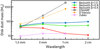 |
Fig. 6 Average dust mass at different wavelengths and with different opacities. The average disk dust mass from our sample is calculated from 1.3-mm, 3-mm, 1-cm, and 2-cm fluxes, assuming optically thin emission, and with different sets of opacity (Beckwith et al. 1990; Zubko et al. 1996; D’Alessio et al. 2001; Birnstiel et al. 2018, with amax = 1 mm). A slightly different number of targets contribute to the individual data points across wavelengths depending on the available photometry. |
4.3 The notable sources in the sample
By construction of the sample, only ordinary objects are treated in this work. As outlined in Sect. 2.1, none of these disks look extremely extended, bright, or asymmetric as, for example, AB Aur, HD 142527, or IRS 48 (Boccaletti et al. 2020; Casassus et al. 2012; van der Marel et al. 2013). Instead, the absence of any large cavity in these disks results in the outer disk being self-shadowed and thus faint in scattered light (Garufi et al. 2017, 2022), with a direct implication on the disk surface density and flaring angle. Nonetheless, the centimeter view of these ordinary objects highlights a few notable cases that are discussed here.
The only sources with an evident disk cavity from the ALMA images by Long et al. (2019) are CIDA 9 and IP Tau. Their free- free emission is low, that is, the second and fifth weakest in the sample. Another source with similarly low free-free emission (third weakest) is DS Tau, hosting a disk where a bright ring accounts for ∼80% of the total ALMA flux. The presence of a central flux component detected by ALMA is the only element that marks a difference in the disk of CIDA 9 and IP Tau. It is therefore tempting to look at the other two of the five sources with low free-free emission. These are V409 Tau and GI Tau, which both host a full compact disk when imaged by ALMA. However, both disks are relatively bright in scattered light given their very low dust mass (similarly to IP Tau; see Garufi et al. 2024), and this morphology may be suggestive of a small-scale cavity that is not resolved by ALMA (that in the case of V409 Tau is also suggested by a small near-IR excess). In fact, recent high-resolution ALMA images of GI Tau reveal a deep disk gap with a central, unresolved component similar to DS Tau (Long et al. in prep.). Therefore, while overall there is no obvious connection between the outer disk morphology and the free-free emission (see Sect. 3.3), the considerations on these five objects seem to highlight a possibly decreased accretion and ejection processes in the presence of a (small-scale) disk inner cavity, as also seen from disks with more prominent disk cavities (Najita et al. 2007, 2015; Manara et al. 2016).
An additional subcategory with peculiar characteristics is that of the massive though compact disks. DO Tau, DQ Tau, and DR Tau all host a disk of 50 au or less in size (lying in the lowest half of the distribution) and with 70 M⊕ or more in dust mass (being among the top five). These sources exhibit three of the four highest free-free emissions and three of the five highest accretion rates of the whole sample. More interestingly, DO Tau and DR Tau are two of the three sources showing evidence of ambient emission from SPHERE (with the third being HP Tau; see below). As shown by Huang et al. (2022) and Winter et al. (2018), DO Tau shows evidence of extended outflow processes and interaction with the environment as well as the nearby star HV Tau. On the other hand, DR Tau shows extended arc-like structures that are reminiscent of an encounter with a cloudlet (Mesa et al. 2022). This may speculatively suggest that the disk of these objects accretes from the environment and that this accreted material may in turn boost the stellar accretion and outflow processes.
On the contrary, the spectroscopic binary DQ Tau does not show any ambient material from the SPHERE image (Garufi et al. 2024). However, this source is known to exhibit strong flares at millimeter wavelengths due to the variable synchrotron emission following magnetic interaction between the individual stars (Salter et al. 2010) or periodic pulsed accretion induced by streamers from the circumbinary disk (Tofflemire et al. 2017). The extremely high flux recorded in our K-band observation (see Fig. A.3) may in principle indicate an episode of outburst within a normal high level of accretion activity. However, this episode should not impact the Ka-band photometry since the two observations were carried out on the same day (12 December, 2021), or alternatively the event should be shorter-lived than a few hours. All this said, it is not surprising that this object represents a challenge for the model (see Sect. 3.3 and Appendix A).
Finally, the case of HP Tau is the most anomalous of the sample. As shown in Sect. 3.3, the very high flux recorded in the Ku band (see Fig. A.3) makes it the only outlier of the trend for the non-dust emission with the accretion rate of Fig. 2. This star is part of a small group with CoKu HP Tau G3 and V1025 Tau and is surrounded by a bright reflection nebula. A clear interaction with the environment is visible from the SPHERE image (Garufi et al. 2024). It is tempting to ascribe the high 2-cm flux to an episode of increased accretion and outflow. However, the stellar light curve only shows minor variability in the visible (half a magnitude from the ASAS-SN survey, Shappee et al. 2014), and no major event is recorded before the VLA observation date (February 2020). Thus, an episodic accretion cannot explain the discrepancy between the accretion rate and the radio flux, leaving open the possibility that the latter is a different type of emission (such as synchrotron emission). Future multiband, multi-epoch radio observations are therefore needed to clarify this case.
5 Summary
This work takes a broad view of the centimeter emission from Class II sources by analyzing a set of 21 objects from the Taurus star-forming region with VLA observations available. Ten of these stars host extended, substructured disks following the classification from the ALMA millimeter survey by Long et al. (2019), while 11 host compact disks with no evidence of resolved substructures. The VLA datasets consist of unresolved or barely resolved images in the Q (7 mm, 9 sources available), Ka (1 cm, 19 sources), K (1.4 cm, 9 sources), Ku (2 cm, all 21 sources), and C (6 cm, 10 sources) bands from which we extracted the photometry. Each source was detected in all bands except the C band, where only two sources were detected.
We fit the SED of the entire sample constructed from the VLA observations plus some literature data spanning from 0.85 mm to 6 cm. The fit includes two power laws to account for the possible non-dust emission at centimeter wavelengths. Our results can be summarized as follows:
The presence of non-dust emission dominating at λ>1 cm is ubiquitously determined in the sample. A spectral slope between 0.3 and 1.1 was characterized by the model suggesting free-free emission from the disk inner regions;
The free-free emission at 2 cm scaled at a same distance correlates well with the accretion rate. This is suggestive of a strong link between the accretion and outflow activities, which is investigated in a forthcoming work. Remarkably, substructured and compact disks are randomly distributed along the trend, indicating that the presence of large-scale disk structures has no impact on the accretion and outflow closer in. Yet, a possible connection for the free-free emission with small-scale cavities may be present;
As much as 35% of the total flux at 2 cm is from the dust, revealing that disks are still relatively bright at these wavelengths. With the SED fit, we can therefore obtain the centimeter dust spectral indices (disentangled from the free- free emission). We find an abrupt change in the median value from 2.4 at the ALMA frequencies to 2.8 in the VLA regime. This change likely sets the transition from optically thick emission (ALMA) to thin emission (VLA);
The distribution of the millimeter and centimeter indices with the disk radial extent by ALMA highlights that the difference between the two is more pronounced for compact disks. This supports the idea of a high optical depth for the inner 40 au up to 3 mm since a larger relative portion of the compact disk provides optically thick millimeter emission compared to a larger disk. Instead, centimeter spectral indices of the two disk categories are similar, suggesting that the grain populations responsible for these indices are analogous in different disk types;
In principle, the disk mass in solids can be refined from the (sub-)centimeter, optically thin emission. However, we emphasize that at 1–2 cm the choice of the dust opacity plays a major role. We show that up to two orders of magnitude different estimates are found from our centimeter flux based on a set of opacities from the literature that assume millimeter maximum grain sizes, which is even larger than at millimeter wavelengths where, nevertheless, the high optical depth plays a major role.
This work contributes to the general effort by the community to characterize less exceptional planet-forming disks with a broader, multiwavelength approach. These VLA observations stress the usefulness of the centimeter emission in studying multiple components of Class II objects and accessing more accurate dust mass and grain properties in their disks. While the moderate resolving power of the current generation of radio telescopes is hampering the employment of this emission, the next decade is promising its full exploitation thanks to the onset of ngVLA and SKA-mid, whereas ALMA Band 1 will already provide useful constraints on the sub-centimeter emission in the near future.
Acknowledgements
We thank the referee for the insightful comments that improved the manuscript, and A. Banzatti and P. Pinilla for very helpful discussions. The National Radio Astronomy Observatory is a facility of the National Science Foundation operated under cooperative agreement by Associated Universities, Inc. This research has made use of the VizieR catalogue access tool, CDS, Strasbourg, France (DOI: 10.26093/cds/vizier). The original description of the VizieR service was published in Ochsenbein et al. (2000). This work was supported by the PRIN-INAF 2019 Planetary Systems At Early Ages (PLATEA) and by the Large Grant INAF 2022 YODA (YSOs Outflows, Disks and Accretion: towards a global framework for the evolution of planet forming systems). The interaction among authors have been appreciably fostered by the INAF mini-grant of the “Bando di finanziamento della Ricerca Fondamentale 2023”. Part of the research activities described in this paper were carried out with contribution of the Next Generation EU funds within the National Recovery and Resilience Plan (PNRR), Mission 4 – Education and Research, Component 2 – From Research to Business (M4C2), Investment Line 3.1 – Strengthening and creation of Research Infrastructures, Project IR0000034 – “STILES – Strengthening the Italian Leadership in ELT and SKA”. C.C.-G. acknowledges support from UNAM DGAPA-PAPIIT grant IG101224 and from CONAHCyT Ciencia de Frontera project ID 86372. C.F.M. and S.F. are funded by the European Union (ERC, WANDA, 101039452 and ERC, UNVEIL, 101076613, respectively). Views and opinions expressed are however those of the author(s) only and do not necessarily reflect those of the European Union or the European Research Council Executive Agency. Neither the European Union nor the granting authority can be held responsible for them. S.F. also acknowledges financial contribution from PRIN-MUR 2022YP5ACE. P.C. acknowledges support by the Italian Ministero dell’Istruzione, Università e Ricerca through the grant Progetti Premiali 2012 – iALMA (CUP C52I13000140001) and by the ANID BASAL project FB210003. Support for F.L. was provided by NASA through the NASA Hubble Fellowship grant #HST-HF2-51512.001-A awarded by the Space Telescope Science Institute, which is operated by the Association of Universities for Research in Astronomy, Incorporated, under NASA contract NAS5-26555. C.J.C. acknowledges support from the Science & Technology Facilities Council (STFC) Consolidated Grant ST/W000997/1. This work has also been supported by the European Union’s Horizon 2020 research and innovation programme under the Marie Sklodowska-Curie grant agreement No. 823823 (DUSTBUSTERS).
Appendix A Individual images and SEDs
The VLA images described in Sect. 3.1 are shown in Fig. A.2. The SED fitting described in Sect. 3.2 yields the parameters listed in Table A.1. All SEDs and relative fits are shown in Fig. A.3. Here we give a brief description of the individual cases referencing the ALMA images by Long et al. (2018, 2019) and the SPHERE images of the scattered light by Garufi et al. (2024).
BP Tau hosts one of the largest compact disks from ALMA with a peculiarly flat inner disk emission. The SPHERE image is clearly asymmetric, with one half of the disk significantly brighter than the other half, which is suggestive of large-angle shadowing. It is the only firm detection in the C band from our survey. Not surprisingly then, the spectral index of the free-free emission is the flattest of the sample (αgas = 0.3).
CIDA 9 has one of the two disks of the sample with a large cavity (with the other being IP Tau). It has a companion at 2.3″ separation that in turns hosts a disk detected by ALMA (Manara et al. 2019) but undetected in our Ku-band VLA image. The primary disk shows the second weakest free-free emission, after V409 Tau. It also has the highest dust spectral index between 1.3 mm and 2 cm (3.1) while the absence of any image at 1 cm prevents from constraining the other relevant indices.
DL Tau is surrounded by one of the three largest disks from the ALMA continuum emission that is nonetheless barely detected by SPHERE since self-shadowed. Multiple rings are visible in the ALMA image. It shows very high accretion and large free-free emission.
DN Tau hosts a standard disk within the sample. The relatively large disk seen by ALMA is barely detected in scattered light. The free-free emission and accretion rates are relatively low.
DO Tau is accompanied by one of the three relatively massive, compact disks (along with DQ Tau and DR Tau). It is a prototypical example of dust spectral index increasing with the wavelength (from α1mm = 2.1 to α2cm = 3.2). The source is enshrouded in a complex environment with evidence of extended outflows and accreting streamers (Huang et al. 2022). The large free-free emission (fourth in the sample), accretion rate (fourth), and near-IR excess (first) all indicate a connection between the environmental and circumstellar processes in act around this source.
DQ Tau is a spectroscopic binary with a stellar mass dynamically measured in 1.2 M⊙ (Czekala et al. 2016). This estimate marginally differs from the photometric value reported in Table 1 (0.5+0.5 M⊙). The disk is another good example of relatively massive though compact disk. The free-free emission constrained by our model is the highest of the sample (HP Tau is not treated by the model). However, in this case we choose to constrain the αgas of the model to 0.6 to prevent the model from determining a very steep value (1.6) that would result in an unnatural 35% of the total emission at 1.33 mm being due to free-free emission. The final fit is much more uncertain than that of the other objects and that most likely reflects the complex environment of the binary system described in Sect. 4.3.
DR Tau has the most massive of the compact disks. Similarly to DO Tau, several arc-like structures in likely interaction with the star are detected around the disk (Mesa et al. 2022). Another analogy with DO Tau is the presence of a high free-free emission, accretion rate, and near-IR excess (third, fifth, and second highest in the sample).
DS Tau hosts a disk with a central component surrounded by a single ring that contains approximately 80% of the total flux. This disk is one of the three mildly inclined disks (60°–70°, along with IQ Tau and V409 Tau), and is barely detected by SPHERE.
SED fit parameters.
FT Tau is surrounded by a disk with a central component surrounded by a bright ring that accounts for about 60% of the total flux (similarly to that of DS Tau).
GI Tau hosts a compact disk with low free-free emission. The disk is one of the least massive disks ever detected in scattered light.
GK Tau has the least massive disk of the sample, together with HQ Tau. It is undetected in scattered light.
GO Tau is surrounded by a disk with a bright, central component and multiple rings further out that however only account for about 20% of the total flux. In fact, the disk is not particularly massive (being averaged in the sample) given its extent (being the largest in the sample). The accretion rate is among the lowest of the sample.
HO Tau has a low-mass compact disk with low free-free emission and accretion rate. The disk has no peculiar feature to be mentioned.
HP Tau hosts an ordinary, compact disk in the ALMA continuum. However, the source is surrounded by a very complex field of arc-like structure that are visible in the SPHERE image and may be due to a recent encounter with nearby companions (see Garufi et al. 2024). The poor available photometry and the anomalously high 2-cm flux prevent any SED fitting.
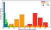 |
Fig. A.1 Free-free over total emission. The fraction of free-free emission over total emission that is obtained from our SED fitting is shown at 1.3 mm, 3 mm, 1 cm, and 2 cm. |
HQ Tau is surrounded by the least massive disk of the sample, together with GK Tau. The disk is marginally detected in scattered light.
IP Tau hosts one of the two disks of the sample with a resolved cavity (with the other being CIDA 9). The disk is relatively bright in scattered light given its very low dust mass, and the SPHERE image reveals evidence of asymmetric structures like spirals in correspondence of the ALMA ring. The source shows very low free-free emission and accretion rate.
IQ Tau has a relatively inclined disk with multiple rings seen by ALMA that is barely visible in the SPHERE image since selfshadowed. Similarly to DL Tau and GO Tau, the ALMA rings account for a small fraction of the total flux.
MWC 480 is the most massive star of the sample (2.1 M⊙) and hosts the most massive disk. The central disk component seen by ALMA is marginally detected by SPHERE as well. It shows the second strongest free-free emission (excluding HP Tau) and the largest mass accretion rate of the sample.
UZ Tau E is a binary star with a total dynamical mass of 1.3 M⊙ (Simon et al. 2000), which is a very discrepant value from the photometric value of Table 1 (0.7 M⊙, although both estimates are quite uncertain). The circumbinary disk exhibits a small, shallow cavity in ALMA encompassed by several rings. The disk is also clearly resolved by SPHERE. The companion UZ Tau W is by itself a binary with 0.4″ separation lying at a separation of 3.5″ from the primary. Both components of UZ Tau W host disks with a similar inclination to that of UZ Tau E (Manara et al. 2019) that are resolved by ALMA and SPHERE, and are detected but unresolved in our VLA Ku-band image.
V409 Tau is surrounded by a compact, inclined disk that is also clearly imaged by SPHERE. It shows the lowest free-free emission, accretion rate, and near-IR excess of the sample.
V836 Tau hosts a compact disk with no notable peculiarity. Yet, the free-free emission is strong (fifth highest value in the sample).
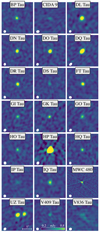 |
Fig. A.2 VLA imagery. All images in the Ku band (2 cm) are shown with the same spatial and color scale (shown to the bottom of the image). The beam size is shown to the bottom left of each panel. |
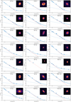 |
Fig. A.3 SED of the entire sample. The inset image is the ALMA continuum image by Long et al. (2019). See Fig. 1 for details. The SED of HP Tau is not fitted because of the poor photometry available. |
Setup and properties of the VLA observations.
Setup and properties of the VLA observations (continued).
References
- ALMA Partnership (Brogan, C. L., et al.) 2015, ApJ, 808, L3 [Google Scholar]
- Andrews, S. M., & Williams, J. P. 2005, ApJ, 631, 1134 [Google Scholar]
- Andrews, S. M., Wilner, D. J., Espaillat, C., et al. 2011, ApJ, 732, 42 [Google Scholar]
- Andrews, S. M., Rosenfeld, K. A., Kraus, A. L., & Wilner, D. J. 2013, ApJ, 771, 129 [Google Scholar]
- Andrews, S. M., Huang, J., Pérez, L. M., et al. 2018, ApJ, 869, L41 [NASA ADS] [CrossRef] [Google Scholar]
- Anglada, G., Rodríguez, L. F., & Carrasco-González, C. 2018, A&A Rev., 26, 3 [Google Scholar]
- Ansdell, M., Williams, J. P., van der Marel, N., et al. 2016, ApJ, 828, 46 [Google Scholar]
- Bae, J., Isella, A., Zhu, Z., et al. 2023, in Astronomical Society of the Pacific Conference Series, 534, Protostars and Planets VII, eds. S. Inutsuka, Y. Aikawa, T. Muto, K. Tomida, & M. Tamura, 423 [NASA ADS] [Google Scholar]
- Bastian, T. S., Benz, A. O., & Gary, D. E. 1998, ARA&A, 36, 131 [Google Scholar]
- Beckwith, S. V. W., & Sargent, A. I. 1991, ApJ, 381, 250 [NASA ADS] [CrossRef] [Google Scholar]
- Beckwith, S. V. W., Sargent, A. I., Chini, R. S., & Guesten, R. 1990, AJ, 99, 924 [Google Scholar]
- Benisty, M., Dominik, C., Follette, K., et al. 2023, in Astronomical Society of the Pacific Conference Series, 534, eds. S. Inutsuka, Y. Aikawa, T. Muto, K. Tomida, & M. Tamura, 605 [NASA ADS] [Google Scholar]
- Birnstiel, T., Dullemond, C. P., Zhu, Z., et al. 2018, ApJ, 869, L45 [CrossRef] [Google Scholar]
- Boccaletti, A., Di Folco, E., Pantin, E., et al. 2020, A&A, 637, L5 [NASA ADS] [CrossRef] [EDP Sciences] [Google Scholar]
- Brown, J. M., Blake, G. A., Qi, C., et al. 2009, ApJ, 704, 496 [Google Scholar]
- Carpenter, J. M., Ricci, L., & Isella, A. 2014, ApJ, 787, 42 [NASA ADS] [CrossRef] [Google Scholar]
- Carrasco-González, C., Henning, T., Chand ler, C. J., et al. 2016, ApJ, 821, L16 [CrossRef] [Google Scholar]
- Carrasco-González, C., Sierra, A., Flock, M., et al. 2019, ApJ, 883, 71 [Google Scholar]
- Casassus, S., Perez M. S., Jordán, A., et al. 2012, ApJ, 754, L31 [NASA ADS] [CrossRef] [Google Scholar]
- Casassus, S., Wright, C. M., Marino, S., et al. 2015, ApJ, 812, 126 [NASA ADS] [CrossRef] [Google Scholar]
- Casassus, S., Marino, S., Lyra, W., et al. 2019, MNRAS, 483, 3278 [Google Scholar]
- Chung, C.-Y., Andrews, S. M., Gurwell, M. A., et al. 2024, ApJS, 273, 29 [NASA ADS] [CrossRef] [Google Scholar]
- Cieza, L. A., Ruíz-Rodríguez, D., Hales, A., et al. 2019, MNRAS, 482, 698 [Google Scholar]
- Crida, A., Morbidelli, A., & Masset, F. 2006, Icarus, 181, 587 [Google Scholar]
- Curone, P., Testi, L., Macías, E., et al. 2023, A&A, 677, A118 [NASA ADS] [CrossRef] [EDP Sciences] [Google Scholar]
- Czekala, I., Andrews, S. M., Torres, G., et al. 2016, ApJ, 818, 156 [NASA ADS] [CrossRef] [Google Scholar]
- D’Alessio, P., Calvet, N., & Hartmann, L. 2001, ApJ, 553, 321 [Google Scholar]
- Dulk, G. A., & Marsh, K. A. 1982, ApJ, 259, 350 [NASA ADS] [CrossRef] [Google Scholar]
- Dullemond, C. P., & Dominik, C. 2004, A&A, 417, 159 [NASA ADS] [CrossRef] [EDP Sciences] [Google Scholar]
- Dutrey, A., Guilloteau, S., & Simon, M. 1994, A&A, 286, 149 [NASA ADS] [Google Scholar]
- Dutrey, A., Guilloteau, S., Duvert, G., et al. 1996, A&A, 309, 493 [NASA ADS] [Google Scholar]
- Dzib, S. A., Loinard, L., Mioduszewski, A. J., et al. 2013, ApJ, 775, 63 [Google Scholar]
- Esplin, T. L., & Luhman, K. L. 2019, AJ, 158, 54 [Google Scholar]
- Fukagawa, M., Tamura, M., Itoh, Y., et al. 2006, ApJ, 636, L153 [Google Scholar]
- Gaia Collaboration (Vallenari, A., et al.) 2023, A&A, 674, A1 [NASA ADS] [CrossRef] [EDP Sciences] [Google Scholar]
- Galli, P. A. B., Loinard, L., Ortiz-Léon, G. N., et al. 2018, ApJ, 859, 33 [Google Scholar]
- Galván-Madrid, R., Liu, H. B., Manara, C. F., et al. 2014, A&A, 570, L9 [NASA ADS] [CrossRef] [EDP Sciences] [Google Scholar]
- Gangi, M., Antoniucci, S., Biazzo, K., et al. 2022, A&A, 667, A124 [NASA ADS] [CrossRef] [EDP Sciences] [Google Scholar]
- Garufi, A., Meeus, G., Benisty, M., et al. 2017, A&A, 603, A21 [NASA ADS] [CrossRef] [EDP Sciences] [Google Scholar]
- Garufi, A., Benisty, M., Pinilla, P., et al. 2018, A&A, 620, A94 [NASA ADS] [CrossRef] [EDP Sciences] [Google Scholar]
- Garufi, A., Avenhaus, H., Pérez, S., et al. 2020, A&A, 633, A82 [NASA ADS] [CrossRef] [EDP Sciences] [Google Scholar]
- Garufi, A., Dominik, C., Ginski, C., et al. 2022, A&A, 658, A137 [NASA ADS] [CrossRef] [EDP Sciences] [Google Scholar]
- Garufi, A., Ginski, C., van Holstein, R. G., et al. 2024, A&A, 685, A53 [NASA ADS] [CrossRef] [EDP Sciences] [Google Scholar]
- Guerra-Alvarado, O. M., Carrasco-González, C., Macías, E., et al. 2024, A&A, 686, A298 [NASA ADS] [CrossRef] [EDP Sciences] [Google Scholar]
- Guidi, G., Isella, A., Testi, L., et al. 2022, A&A, 664, A137 [NASA ADS] [CrossRef] [EDP Sciences] [Google Scholar]
- Guzmán, V. V., Öberg, K. I., Carpenter, J., et al. 2018, ApJ, 864, 170 [CrossRef] [Google Scholar]
- Harsono, D., Long, F., Pinilla, P., et al. 2024, ApJ, 961, 28 [NASA ADS] [CrossRef] [Google Scholar]
- Huang, J., Ginski, C., Benisty, M., et al. 2022, ApJ, 930, 171 [NASA ADS] [CrossRef] [Google Scholar]
- Isella, A., Chandler, C. J., Carpenter, J. M., Pérez, L. M., & Ricci, L. 2014, ApJ, 788, 129 [NASA ADS] [CrossRef] [Google Scholar]
- Isella, A., Huang, J., Andrews, S. M., et al. 2018, ApJ, 869, L49 [NASA ADS] [CrossRef] [Google Scholar]
- Kenyon, S. J., Gómez, M., & Whitney, B. A. 2008, in Handbook of Star Forming Regions, Volume I, 4, ed. B. Reipurth, 405 [NASA ADS] [Google Scholar]
- Kley, W. 1999, MNRAS, 303, 696 [NASA ADS] [CrossRef] [Google Scholar]
- Lada, C. J. 1987, in IAU Symposium, 115, Star Forming Regions, eds. M. Peimbert, & J. Jugaku, 1 [NASA ADS] [Google Scholar]
- Lesur, G., Flock, M., Ercolano, B., et al. 2023, in Astronomical Society of the Pacific Conference Series, 534, Protostars and Planets VII, ed. S. Inutsuka, Y. Aikawa, T. Muto, K. Tomida, & M. Tamura, 465 [NASA ADS] [Google Scholar]
- Lin, C.-L., Ip, W.-H., Hsiao, Y., et al. 2023, AJ, 166, 82 [NASA ADS] [CrossRef] [Google Scholar]
- Liu, H. B., Muto, T., Konishi, M., et al. 2024, A&A, 685, A18 [NASA ADS] [CrossRef] [EDP Sciences] [Google Scholar]
- Lommen, D., Maddison, S. T., Wright, C. M., et al. 2009, A&A, 495, 869 [NASA ADS] [CrossRef] [EDP Sciences] [Google Scholar]
- Long, F., Pinilla, P., Herczeg, G. J., et al. 2018, ApJ, 869, 17 [Google Scholar]
- Long, F., Herczeg, G. J., Harsono, D., et al. 2019, ApJ, 882, 49 [Google Scholar]
- Macías, E., Anglada, G., Osorio, M., et al. 2016, ApJ, 829, 1 [Google Scholar]
- Macías, E., Anglada, G., Osorio, M., et al. 2017, ApJ, 838, 97 [Google Scholar]
- Macías, E., Espaillat, C. C., Ribas, Á., et al. 2018, ApJ, 865, 37 [Google Scholar]
- Macías, E., Guerra-Alvarado, O., Carrasco-González, C., et al. 2021, A&A, 648, A33 [EDP Sciences] [Google Scholar]
- Manara, C. F., Rosotti, G., Testi, L., et al. 2016, A&A, 591, L3 [NASA ADS] [CrossRef] [EDP Sciences] [Google Scholar]
- Manara, C. F., Morbidelli, A., & Guillot, T. 2018, A&A, 618, L3 [NASA ADS] [CrossRef] [EDP Sciences] [Google Scholar]
- Manara, C. F., Tazzari, M., Long, F., et al. 2019, A&A, 628, A95 [NASA ADS] [CrossRef] [EDP Sciences] [Google Scholar]
- Marino, S., Casassus, S., Perez, S., et al. 2015, ApJ, 813, 76 [NASA ADS] [CrossRef] [Google Scholar]
- Mesa, D., Ginski, C., Gratton, R., et al. 2022, A&A, 658, A63 [NASA ADS] [CrossRef] [EDP Sciences] [Google Scholar]
- Miotello, A., Kamp, I., Birnstiel, T., Cleeves, L. C., & Kataoka, A. 2023, in Astronomical Society of the Pacific Conference Series, 534, Protostars and Planets VII, eds. S. Inutsuka, Y. Aikawa, T. Muto, K. Tomida, & M. Tamura, 501 [NASA ADS] [Google Scholar]
- Mulders, G. D., Pascucci, I., Ciesla, F. J., & Fernandes, R. B. 2021, ApJ, 920, 66 [NASA ADS] [CrossRef] [Google Scholar]
- Najita, J. R., Strom, S. E., & Muzerolle, J. 2007, MNRAS, 378, 369 [NASA ADS] [CrossRef] [Google Scholar]
- Najita, J. R., Andrews, S. M., & Muzerolle, J. 2015, MNRAS, 450, 3559 [NASA ADS] [CrossRef] [Google Scholar]
- Norfolk, B. J., Maddison, S. T., Pinte, C., et al. 2021, MNRAS, 502, 5779 [Google Scholar]
- Panagia, N., & Felli, M. 1975, A&A, 39, 1 [Google Scholar]
- Pascucci, I., Gorti, U., & Hollenbach, D. 2012, ApJ, 751, L42 [Google Scholar]
- Pascucci, I., Testi, L., Herczeg, G. J., et al. 2016, ApJ, 831, 125 [Google Scholar]
- Pérez, L. M., Chandler, C. J., Isella, A., et al. 2015, ApJ, 813, 41 [CrossRef] [Google Scholar]
- Pinilla, P., Birnstiel, T., Ricci, L., et al. 2012, A&A, 538, A114 [NASA ADS] [CrossRef] [EDP Sciences] [Google Scholar]
- Pinilla, P., Benisty, M., Birnstiel, T., et al. 2014, A&A, 564, A51 [NASA ADS] [CrossRef] [EDP Sciences] [Google Scholar]
- Pollack, J. B., Hubickyj, O., Bodenheimer, P., et al. 1996, Icarus, 124, 62 [NASA ADS] [CrossRef] [Google Scholar]
- Reynolds, S. P. 1986, ApJ, 304, 713 [NASA ADS] [CrossRef] [Google Scholar]
- Ribas, Á., Espaillat, C. C., Macías, E., & Sarro, L. M. 2020, A&A, 642, A171 [NASA ADS] [CrossRef] [EDP Sciences] [Google Scholar]
- Ricci, L., Testi, L., Natta, A., & Brooks, K. J. 2010, A&A, 521, A66 [NASA ADS] [CrossRef] [EDP Sciences] [Google Scholar]
- Ricci, L., Rome, H., Pinilla, P., et al. 2017, ApJ, 846, 19 [CrossRef] [Google Scholar]
- Rodríguez, L. F., Anglada, G., & Curiel, S. 1999, ApJS, 125, 427 [Google Scholar]
- Rota, A. A., Meijerhof, J. D., van der Marel, N., et al. 2024, A&A, 684, A134 [NASA ADS] [CrossRef] [EDP Sciences] [Google Scholar]
- Salter, D. M., Kóspál, Á., Getman, K. V., et al. 2010, A&A, 521, A32 [NASA ADS] [CrossRef] [EDP Sciences] [Google Scholar]
- Sanchez, M., van der Marel, N., Lambrechts, M., Mulders, G. D., & Guerra-Alvarado, O. M. 2024, A&A, 689, A236 [NASA ADS] [CrossRef] [EDP Sciences] [Google Scholar]
- Shappee, B. J., Prieto, J. L., Grupe, D., et al. 2014, ApJ, 788, 48 [Google Scholar]
- Sierra, A., & Lizano, S. 2020, ApJ, 892, 136 [Google Scholar]
- Simon, M., Dutrey, A., & Guilloteau, S. 2000, ApJ, 545, 1034 [NASA ADS] [CrossRef] [Google Scholar]
- Tazzari, M., Clarke, C. J., Testi, L., et al. 2021a, MNRAS, 506, 2804 [NASA ADS] [CrossRef] [Google Scholar]
- Tazzari, M., Testi, L., Natta, A., et al. 2021b, MNRAS, 506, 5117 [NASA ADS] [CrossRef] [Google Scholar]
- Testi, L., Birnstiel, T., Ricci, L., et al. 2014, Protostars and Planets VI, 339 [Google Scholar]
- Tofflemire, B. M., Mathieu, R. D., Ardila, D. R., et al. 2017, ApJ, 835, 8 [CrossRef] [Google Scholar]
- Tripathi, A., Andrews, S. M., Birnstiel, T., & Wilner, D. J. 2017, ApJ, 845, 44 [Google Scholar]
- Ubach, C., Maddison, S. T., Wright, C. M., et al. 2012, MNRAS, 425, 3137 [NASA ADS] [CrossRef] [Google Scholar]
- Ubach, C., Maddison, S. T., Wright, C. M., et al. 2017, MNRAS, 466, 4083 [NASA ADS] [Google Scholar]
- van der Marel, N. 2023, Eur. Phys. J. Plus, 138, 225 [NASA ADS] [CrossRef] [Google Scholar]
- van der Marel, N., & Mulders, G. D. 2021, AJ, 162, 28 [NASA ADS] [CrossRef] [Google Scholar]
- van der Marel, N., & Pinilla, P. 2023, arXiv e-prints [arXiv:2310.09077] [Google Scholar]
- van der Marel, N., van Dishoeck, E. F., Bruderer, S., et al. 2013, Science, 340, 1199 [Google Scholar]
- Winter, A. J., Booth, R. A., & Clarke, C. J. 2018, MNRAS, 479, 5522 [Google Scholar]
- Wright, C. M., Maddison, S. T., Wilner, D. J., et al. 2015, MNRAS, 453, 414 [NASA ADS] [CrossRef] [Google Scholar]
- Xin, Z., Espaillat, C. C., Rilinger, A. M., Ribas, Á., & Macías, E. 2023, ApJ, 942, 4 [NASA ADS] [CrossRef] [Google Scholar]
- Zhu, Z., Zhang, S., Jiang, Y.-F., et al. 2019, ApJ, 877, L18 [NASA ADS] [CrossRef] [Google Scholar]
- Zubko, V. G., Mennella, V., Colangeli, L., & Bussoletti, E. 1996, MNRAS, 282, 1321 [Google Scholar]
Due to the conversion to the intrinsic spatial scale, two substructured disks (around IP and FT Tau) are actually smaller than the largest compact disk (in DR Tau).
Here, we use a disk extent of 50 au to discriminate between the two categories. This criterion is nearly identical to the substructured versus compact-disk classification, except for the massive but formally compact disk of DR Tau (see Sect. 2.1). Also, DQ Tau has been removed from this analysis in view of the large uncertainty at centimeter wavelengths, which leads to anomalously high fluxes (see Sect. 4.3 and Appendix A).
All Tables
All Figures
|
Fig. 1 Illustrative SED. The observed photometry of DR Tau is fit by two power laws for the dust continuum and the free-free emission. All derived slopes and all SEDs are shown in Table A.1 and Fig. A.3, respectively. |
| In the text | |
|
Fig. 2 Free-free emission versus mass accretion rate. The free-free emission at 2 cm constrained by our model (see Sect. 3.2) for the entire sample is scaled to 140 pc and compared with the mass-accretion rates shown in Table 1. Despite large errors, a correlation between both quantities is clearly seen across several orders of magnitude. Nonetheless, the distribution of compact disks against substructured disks appears random. HP Tau (with a free-free emission at 140 pc of approximately 10 mJy and an accretion rate of 2.5 ⋅ 10−11 M⊙ yr−1) clearly falls out of the correlation and is not shown in order to provide a better view of the plot. |
| In the text | |
|
Fig. 3 Millimeter and centimeter dust spectral indices. The individual α at four different spectral ranges are shown in semi-transparency. These are obtained by removing the free-free emission from our photometry and comparing with literature values (see text). The big foreground symbols are the average values for the entire sample. The error bars of the individual sources are inherited from the uncertainty on the photometry, while those of the averages are the dispersion of the relative sample. The red line indicates the spectral index of the interstellar dust grains in the millimeter index, while the blue line shows the expected index from optically thick emission. |
| In the text | |
|
Fig. 4 Dust spectral indices versus disk extent. All available α of our sample obtained after removing the free-free emission are compared with the disk extent from the ALMA continuum emission at 1.3 mm listed in Table 1. The best fits to the data are shown as dashed lines. A small offset in extent is given to some datapoints so that indices at the same radius, when available, are from the same object. |
| In the text | |
|
Fig. 5 Total flux ratio between substructured and compact disks at different wavelengths. The average dust-integrated flux at the same distance of compact disks from 1.3-mm, 3-mm, 1-cm, and 2-cm fluxes is confronted with that of substructured disks. Fluxes at 7 mm are not shown, because the subsamples are too small. The red points indicate the fluxes integrated over the inner 40 au from the ALMA highly resolved images. At 1.3 mm, the compact disks have relatively lower fluxes than at the other wavelengths, while a similar value (50%–60%) is found when considering only the inner 40 au, suggesting that the emission from this disk region is severely optically thick. |
| In the text | |
|
Fig. 6 Average dust mass at different wavelengths and with different opacities. The average disk dust mass from our sample is calculated from 1.3-mm, 3-mm, 1-cm, and 2-cm fluxes, assuming optically thin emission, and with different sets of opacity (Beckwith et al. 1990; Zubko et al. 1996; D’Alessio et al. 2001; Birnstiel et al. 2018, with amax = 1 mm). A slightly different number of targets contribute to the individual data points across wavelengths depending on the available photometry. |
| In the text | |
|
Fig. A.1 Free-free over total emission. The fraction of free-free emission over total emission that is obtained from our SED fitting is shown at 1.3 mm, 3 mm, 1 cm, and 2 cm. |
| In the text | |
|
Fig. A.2 VLA imagery. All images in the Ku band (2 cm) are shown with the same spatial and color scale (shown to the bottom of the image). The beam size is shown to the bottom left of each panel. |
| In the text | |
|
Fig. A.3 SED of the entire sample. The inset image is the ALMA continuum image by Long et al. (2019). See Fig. 1 for details. The SED of HP Tau is not fitted because of the poor photometry available. |
| In the text | |
Current usage metrics show cumulative count of Article Views (full-text article views including HTML views, PDF and ePub downloads, according to the available data) and Abstracts Views on Vision4Press platform.
Data correspond to usage on the plateform after 2015. The current usage metrics is available 48-96 hours after online publication and is updated daily on week days.
Initial download of the metrics may take a while.