| Issue |
A&A
Volume 694, February 2025
|
|
|---|---|---|
| Article Number | A148 | |
| Number of page(s) | 13 | |
| Section | Interstellar and circumstellar matter | |
| DOI | https://doi.org/10.1051/0004-6361/202452010 | |
| Published online | 07 February 2025 | |
Are stellar embryos in Perseus radio-synchrotron emitters?
Statistical data analysis with Herschel and LOFAR paving the way for the SKA
1
INAF – Osservatorio Astrofisico di Arcetri,
Largo E. Fermi 5,
50125
Firenze,
Italy
2
Laboratoire de Physique de l’Ecole Normale Supérieure, ENS, Université PSL, CNRS, Sorbonne Université, Université de Paris,
75005
Paris,
France
3
Istituto di Astrofisica e Planetologia Spaziali (IAPS), INAF,
Via Fosso del Cavaliere 100,
00133
Roma,
Italy
4
Thüringer Landessternwarte,
Sternwarte 5,
07778
Tautenburg,
Germany
★ Corresponding author; This email address is being protected from spambots. You need JavaScript enabled to view it.
Received:
27
August
2024
Accepted:
29
November
2024
Abstract
Cosmic rays (CRs) are crucial to the chemistry and physics of star-forming regions. By controlling the ionization rate of molecular gas, they mediate the interaction between matter flows and interstellar magnetic fields, thereby regulating the entire star formation process, from the diffuse interstellar medium to the formation of stellar embryos, or cores. The electronic GeV component of CRs is expected to generate nonthermal synchrotron radiation, which should be detectable at radio frequencies across multiple physical scales. However, synchrotron emission from star-forming regions in the Milky Way has barely been observed to date. In this work, we present the first attempt to statistically detect synchrotron emission with the LOw Frequency ARray (LOFAR) at 144 MHz from the nearby Perseus molecular cloud (at a distance of ~300 pc). We perform median stacking over 353 prestellar and 132 protostellar cores derived from the Herschel Gould Belt Survey. Using data from the LOFAR two meter sky survey (LoTSS) with an angular resolution of 20″, we identify 18 potential protostellar candidates and 5 prestellar ones. However, we interpret these as extragalactic contamination in the Herschel catalog. Our statistical analysis of the remaining cores does not reveal any significant radio counterpart of prestellar and protostellar cores at levels of 5 μJy beam−1 and 8 μJy beam−1 in the stacked maps, respectively. We discuss our non-detections in two ways. For protostellar cores, we believe that strong extinction mechanisms of radio emission, such as free-free absorption and the Razin–Tsytovich effect, may be at play. For prestellar cores, using analytical models of magnetostatic–isothermal cores, the lack of detection with LOFAR helps us constrain the maximum ordered magnetic-field strength statistically attainable by these objects, on the order of 100 μJG. We predict that the statistical emission of the prestellar-core sample in Perseus seen by LoTSS should be detectable in only 9 hours and 4 hours with the Square Kilometre Array-Low (SKA-Low) array assemblies AA* and AA4, respectively.
Key words: radiation mechanisms: non-thermal / methods: statistical / stars: formation / stars: protostars / cosmic rays / ISM: magnetic fields
© The Authors 2025
 Open Access article, published by EDP Sciences, under the terms of the Creative Commons Attribution License (https://creativecommons.org/licenses/by/4.0), which permits unrestricted use, distribution, and reproduction in any medium, provided the original work is properly cited.
This article is published in open access under the Subscribe to Open model. This email address is being protected from spambots. You need JavaScript enabled to view it. to support open access publication.
1 Introduction
The formation of solar-type stars is determined by highly nonlinear physical processes (e.g., Ballesteros-Paredes et al. 2020). The self-gravity of matter overdensities is contrasted by turbulent and magnetized flows in the interstellar medium (ISM), driving the evolution of diffuse multiphase gas into dense and filamentary molecular clouds where stellar embryos, or cores, originate (see recent reviews by Hennebelle & Inutsuka 2019 and Pattle et al. 2023). These cores evolve from gravitationally unstable prestellar cores to main-sequence objects through a series of protostellar phases, during which the core mass progressively accretes from the core envelope onto the central source (e.g., Andre et al. 2000).
Magnetic fields are believed to regulate this multi-scale flow of matter, from filaments in molecular clouds (e.g., Planck Collaboration Int. XXXII 2016; Planck Collaboration Int. XXXV 2016; Soler 2019; Hacar et al. 2023) down to the scale of protostellar cores (e.g., Maury et al. 2022). The magnetic-field strength increases from a few μJG in the diffuse ISM (for total gas column densities, NH < 5 × 1021 cm−2, Heiles & Troland 2003; Thompson et al. 2019) to hundreds of mG in denser regions (NH ~ 1024 cm−2, Crutcher et al. 2010), where most cores appear slightly supercritical with respect to magnetic support, and thus inclined toward gravitational collapse (e.g., Crutcher 2012).
The transition to supercritical cores must occur at the expense of some diffusion process that decouples the contrasting effect of magnetic pressure against gravity, such as ambipolar diffusion, which is the relative dynamical drift of ions and neutrals in nonideal magnetohydrodynamic (MHD) flows (e.g., Pinto et al. 2008; Momferratos et al. 2014). Thus, one key parameter of the star formation process is the amount of available ionized particles in molecular clouds to link the matter flow with magnetic fields. While ultraviolet (UV) radiation is considered the most powerful ionizing source in the diffuse ISM, cosmic rays (CRs) – of either interstellar or local origin – are believed to be the main contributors to the ionization of the dense, UV-shielded portions of molecular clouds (e.g., Grenier et al. 2015; Padovani et al. 2020). Cosmic ray ionization is primarily determined by the properties of MeV protons (e.g., Gabici 2022). Cosmic ray electrons (CRe), while still relevant for the ionization rate of molecular clouds in the MeV range (Ivlev et al. 2021; Padovani et al. 2022), are mainly expected to generate nonthermal synchrotron radiation as they gyrate around magnetic-field lines in the GeV range. However, this nonthermal emission from molecular clouds in the Milky Way has been observed in the radio band at low frequencies (below 1 GHz) in only a few instances, such as the diffuse emission in the Orion-Taurus ridge (Bracco et al. 2023) and in the compact regions around the protostellar jet of DG Tau A (Feeney-Johansson et al. 2019). The lack of synchrotron emission from molecular clouds represents a long-standing problem that challenges our understanding of CRe and magnetic fields in star-forming regions (Dickinson et al. 2015).
With the advent of groundbreaking observational facilities, such as the Square Kilometre Array (SKA, Dewdney et al. 2009), we may finally reach the sensitivity required to detect the expected synchrotron emission from individual objects (e.g., Padovani & Galli 2018). For the first time in this study, we attempt to reveal this emission statistically by performing median stacking over a large sample of prestellar and protostellar cores. In prestellar cores, CRe have an interstellar origin, whereas in protostellar cores, they are expected to be locally accelerated by internal sources, such as jets and shocks (Padovani et al. 2015, 2016). We combine data at 144 MHz from the LOw Frequency ARray (LOFAR, van Haarlem et al. 2013) with the most extensive catalog of cores in the nearby star-forming region of Perseus, which were revealed in the infrared by the Herschel satellite (Pilbratt et al. 2010).
The paper is organized as follows. In Sect. 2, we introduce the data and detail the stacking procedure. In Sect. 3, we present our main results on the stacking of LOFAR data over the Herschel samples of cores. In Sect. 4, we discuss our results in the context of prestellar and protostellar cores, separately. The paper is summarized in Sect. 5 and contains two appendices (Appendices A and B).
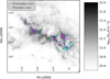 |
Fig. 1 Column density map of molecular hydrogen, NH2, combining Herschel and Planck data of the Perseus molecular cloud. Magenta and cyan circles correspond to protostellar and prestellar cores, respectively, as they are defined in P21. |
2 Data and methods
In this section, we describe the Herschel and LOFAR data used in the analysis and the basic principles of the stacking employed to search for the radio emission of the Perseus cores.
2.1 Herschel data
We considered the catalog of prestellar and protostellar cores in the Perseus molecular cloud released by the Herschel Gould Belt Survey (HGBS) and detailed in Pezzuto et al. (2021), hereafter P21. The cores were identified on the basis of their spectral energy distribution (SED) properties using Herschel data between 70 μm and 500 μm. Two samples of 132 protostellar and 353 prestellar cores have been made available via the VizieR data archive1. We note that, to increase the statistical sample, we included all candidate prestellar cores, even those labeled as tentative detections in the Herschel catalog. However, we confirm that our results remain unchanged when these are excluded.
In Fig. 1, we show the location of the full set of cores over the multi-resolution H2 column-density map of the Perseus molecular cloud. This map has a variable angular resolution between 18″ and 5′. It was obtained by combining data from the Herschel2 (André et al. 2010) and Planck (Planck Collaboration I 2016) satellites to recover the diffuse dust emission in the periphery of the HGBS molecular clouds, surveyed at low resolution with Planck, while preserving dense, high-resolution regions observed by Herschel (Bracco et al. 2020). While most of the prestellar cores (cyan) are located within the densest regions of the molecular cloud, protostellar cores (magenta) appear more dispersed, even in the diffuse parts of Perseus.
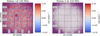 |
Fig. 2 Stokes I and V maps of the Perseus molecular cloud from the LoTSS survey. The maps have the same projection and grid as the NH2 map shown in Fig. 1, centered on the celestial coordinate (RA, Dec) (J2000) = (54°, +31°). |
2.2 LOFAR data
To look for the meter-wavelength radio emission of the Herschel cores, we used 20″ resolution Stokes I and V maps at 144 MHz from the latest internal data release of the LOFAR Two-meter Sky Survey (LoTSS, Shimwell et al. 2022). LoTSS is a wide-area deep radio wavelength sky survey. Most pointings are observed for a total of 8 hours with 48 MHz (120–168 MHz centered at 144 MHz) of bandwidth which allows for two pointings to be observed simultaneously with current LOFAR capabilities. The data are processed with a direction-independent (DI) calibration pipeline that is executed on computer facilities at Forschungszentrum Jülich and SURF (Drabent et al. 2019). The DI calibration pipeline used for the data processing is described in van Weeren et al. (2016) and Williams et al. (2016) and makes use of several software packages including the Default Pre-Processing Pipeline (DP3, van Diepen et al. 2018), LOFAR SolutionTool (LoSoTo, de Gasperin et al. 2019) and AOFlagger (Offringa et al. 2012). The pipeline corrects for DI errors such as the clock offsets between different stations, ionospheric Faraday rotation, the offset between XX and YY phases and amplitude calibration solutions (de Gasperin et al. 2019). The Scaife & Heald (2012) flux density scale is used for the amplitude calibration together with the TIFR GMRT Sky Survey alternative data release sky models (Intema et al. 2017) of the target fields for an initial phase calibration, although both the amplitude and phase calibration are refined during subsequent processing.
A direction-dependent (DD) calibration and imaging pipeline follows the DI phase. The DD routine makes use of kMS (Tasse 2014; Smirnov & Tasse 2015) for DD calibration, and of DDFacet (Tasse et al. 2018) to apply the DD solutions during imaging. Finally, the restoring beam used in DDFacet for each image product type is kept constant and all image products are made with a uv-minimum baseline of 100 m with the uv-maximum baselines varied to provide images at different resolutions – the highest 6″ resolution images use baselines of up to 120 km (i.e. all LOFAR stations within the Netherlands; for more details on LoTSS, refer to Shimwell et al. 2017, Shimwell et al. 2019, and Shimwell et al. 2022).
For our purposes, as is described in Appendix A, we produced a mosaic of five pointings in the surroundings of Perseus reaching a uniform root mean square (RMS) value in Stokes V between 0.1 and 0.2 mJy beam−1 in the molecular cloud, where NH2 > 1021 cm−2 (see Fig. A.3). Because of resolved and unresolved (confusion noise) point sources, it is difficult to estimate the noise level in Stokes I. On the contrary, Stokes V is considered a good tracer of the thermal noise in radio-interferometric data. In Fig. 2, we show the final LOFAR maps used in this work without primary-beam corrections that allow us to access the calibrated fluxes in Stokes I. This explains the increase in noise at the edges of the images. The maps are on the same grid as the NH2 map shown in Fig. 1. In the Stokes I map, there is a noticeable intense circular structure at the center, which is the result of contamination from a bright-source calibration residual.
2.3 Stacking analysis
We aim to explore whether we can detect LOFAR intensity at the positions of the cores listed in P21. To this end, we decided to stack Stokes I and V cutout maps centered on each prestellar and protostellar core separately. While searching for Stokes I counterparts, we used Stokes V as noise reference (see Sect. 2.2). The LOFAR maps at hand have a pixel size of 4.5″. Since we do not resolve the cores, we aim to extract LOFAR intensities within the nominal full width at half maximum (FWHM) of 20″. We produced sufficiently large cutouts made of 80-pixel-squared maps.
The stacking procedure was twofold. For all cutout maps outside a circle of a 5-pixel radius from the center (roughly twice the size of the FWHM – see black circle in Fig. 3), we performed a median stacking, which is less contaminated by strong outlier sources compared to the mean (e.g., Lee et al. 2010). This choice is justified because outside the center of the stacked maps, we are primarily interested in measuring a meaningful noise level. For the central pixels around the positions of the cores, we instead applied a mean stacking, as we aim to find correspondence between the Herschel cores and any bright source detected with LOFAR.
The resulting stacked maps for both prestellar and protostellar cores are shown in Fig. 3. A black circle at the center separates the central region, where we applied the mean stacking, from the outer region, where we used the median stacking. We note that the median stacking in Stokes I is biased toward positive values compared to Stokes V, which fluctuates around zero. This bias, which would be even stronger with mean stacking, is caused by the presence of a few outlier sources at each position in the cutout maps. The bias is homogeneous across the residual stacked maps, measuring 27 μJy beam−1 for protostellar cores and 24 μJy beam−1 for prestellar cores. In the following, we remove the respective biases from the stacked maps.
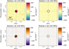 |
Fig. 3 Stacked maps of Stokes I (left) and V (right) from LOFAR at 144 MHz for protostellar (top) and prestellar (bottom) cores in the Perseus molecular cloud. The synthetized beam of 20″ FWHM is shown with a white circle in the top left panel. The central region where the mean stacking is performed is shown in all panels by the black circle at the center, which is twice the size of the FWHM. At the distance of Perseus (~300 pc), 90″ corresponds to ~0.15 pc. |
3 Results
In this section, we report the main results of our study on the stacked maps, the source characterization, and the analysis of the residual stacked maps.
3.1 Central excess in the stacked Stokes I maps
As is shown in Fig. 3, we detect a clear central excess in the stacked Stokes I maps that is not present in Stokes V, both in the case of prestellar and protostellar cores. Since we performed a mean stacking at the center, we now explore whether the excess is a statistical property of the Herschel cores or the contribution of a few bright sources.
For each cutout map, we computed the ratio (ℛ) between the mean of Stokes I within the central region and the corresponding RMS value of Stokes V in the outer region. The resulting ℛ values are shown in Fig. 4 for both prestellar and protostellar cores as a function of the RA coordinate of each core in degrees. In the top panels of the figure, we also show the corresponding RMS values of V, which are consistent with the RMS values of the mosaic, as is described in Sect. 2.2 and shown in Fig. A.3.
For both types of cores, we define as outliers those with ℛ > 3 (dashed red line), or the 16% and the 5% of the protostellar and prestellar cores, respectively. To verify the robustness of this threshold, in the following we shall also consider the case with ℛ > 2 (dashed blue line), or the 18% and the 7% of the protostellar and prestellar core samples. All outlier-maps with ℛ > 3 can be seen in Figs. B.1 and B.2. By selecting the outliers with intensity peaks at the center of each cutout, we detected 18 protostellar cores and 5 prestellar cores that are listed in Table 1, or 14% and 1% of the corresponding samples of cores.
3.2 Characterization of the selected bright cores
In order to assess the robustness of the correlation between these 23 Herschel cores with LOFAR against the contamination of extragalactic sources, we searched the literature for multiwavelength catalogs. Using the SIMBAD-CDS astronomical database and the Aladin sky viewer (Boch & Fernique 2014), we looked for emission in the optical with Pan-STARRS1 (Magnier et al. 2020), in the near-infrared (NIR) with 2MASS (Skrutskie et al. 2006) and Spitzer (Dunham et al. 2008; Evans et al. 2009), and in the cm-radio range with the VLA (Condon et al. 1998; Tobin et al. 2016). We also searched the NASA/IPAC Extra-galactic Database (NED, Chen et al. 2022).
In Table 1, we list the selected protostellar and prestellar cores as reported in P21, along with their names and locations. We also specify their indices (internal to this work) and their multiwavelength counterparts. If a core is detected within the LOFAR FWHM in the other datasets, it is marked with a “Y”; if not detected, it is marked with an “N”. Uncertain cases are indicated with “Y/N”. For each core, the star symbol “*” indicates that the core is absent as a known source in SIMBAD-CDS, and the label “‡” indicates that it is present in NED.
All protostellar cores with detected LOFAR emission at the center are listed in NED, with the closest counterpart being within only 5″. These cores also emit in the optical, NIR, and cm-radio ranges. However, aside from a few cases with clear extended emission (e.g., indices 97 and 113), which are likely external galaxies, it is challenging to determine whether the origin of the remaining cores is Galactic or extragalactic. The cores without the “*” symbol are cataloged as young stellar objects, although with a low confidence level and a high likelihood of being contaminating galaxies (Section 5.2 in Dunham et al. 2008). This evidence leads us to surmise that the LOFAR excess corresponding to the protostellar cores detected by P21 is generally the result of background emission from external galaxies.
In the case of prestellar cores, the correlation between the Herschel and LOFAR data is even poorer than in the protostellar case. Some of them, as shown in Fig. B.2, are likely signatures of jets from radio galaxies given their extended bipolar morphology. Additionally, despite not emitting either NIR or optical radiations, as is expected in the case of prestellar cores, the sample of five candidate cores is present in NED. Finally, as will be discussed in Sect. 4.2, the current theoretical understanding of nonthermal synchrotron radiation in prestellar cores struggles to reproduce the mJy beam−1 levels observed in LOFAR. For all these reasons, we conclude that the central excess found in prestellar cores is due to contamination from external galaxies. We verified that all sources listed as galaxies in P21 (see their Table E.1) exhibit a central excess in LOFAR Stokes I at the level of a mJy beam−1.
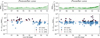 |
Fig. 4 Ratio (ℛ) between the mean of Stokes I within the central region (black circle in Fig. 3) and the RMS value of Stokes V in the outer region (see top panels), for prestellar (right) and protostellar (left) cores. ℛ is shown as a function of the RA coordinate of each core. The selected sources correspond to ℛ values greater than 2 (black dots above the dashed blue line) and 3 (red dots above the dashed red line). |
3.3 Residual stacked maps
We repeated the stacking analysis after excluding the contaminating extragalactic sources from the core catalog. In Fig. 5, we show the residual stacked maps for both prestellar and protostellar cores, where the central excess is now removed for both types of cores. We obtained residual stacked maps of Stokes I that closely resemble noise if compared to Stokes V. This is supported by comparing the normalized distribution functions (NDFs) of the residual stacked maps. In Fig. 6, we show the NDF – both as histograms and as kernel density estimates (KDEs) – of the averaged Stokes I (in blue) and Stokes V (in purple) within 5000 circles of equal area to the central region delimited by the black circle in, for instance, Figs. 3 and 5. These circles are uniform-randomly distributed over the maps. As was expected in the case of noise, the NDFs are consistent with zero within 1-σ for both prestellar and protostellar cores, and for both Stokes I and Stokes V residual stacked maps. Since the sample of prestellar cores is much larger than that of protostellar cores (348 versus 114), the corresponding NDFs are generally narrower. The 84th percentile values of the Stokes I NDFs are 5 μJy beam−1 for prestellar cores and 8 μJy beam−1 for protostellar cores. We also note that the NDF of Stokes I is broader than that of Stokes V, as Stokes I is more sensitive to calibration uncertainties – because of the large amount of point sources – than Stokes V, which should be dominated by thermal noise (Shimwell et al. 2022).
Finally, in Fig. 6, we show with diagonal black hatches the range of average values of the residual stacked maps within the central region considering both ℛ > 2 and >3. While in the protostellar case this average is well within 1-σ of the corresponding NDF, for prestellar cores, the case with ℛ > 3 slightly falls above the 84th percentile. However, the significance of this result is marginal, given the stronger influence of outlier sources in the mean stacking applied to the central region compared to the median stacking used in the outer region, as is shown by the case with ℛ > 3. Overall, our statistical analysis fails to detect any significant emissions from prestellar and protostellar cores at meter wavelengths.
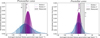 |
Fig. 6 Normalized distribution functions for protostellar (left) and prestellar (right) cores of the residual stacked Stokes-I (blue) and -V (purple) maps averaged within 5000 circles of equal area as the central black circle in Figs. 3 and 5. The measured values at the center are shown with diagonal black hatches depending on the choice of ℛ for defining the outlier cores. From dark to light colours, shadows correspond to 1-, 2-, and 3-σ levels. The 84 th percentiles are 8 μJy beam−1 and 5 μJy beam−1 for protostellar and prestellar cores, respectively. The NDF are shown with both histograms and kernel density estimates. |
4 Discussion
In this section, we investigate several scenarios that might explain why no statistical signature of stellar embryos in Perseus was found using LOFAR. We divide the discussion into two parts: protostellar cores (Sect. 4.1) and prestellar cores (Sect. 4.2).
4.1 Extinction mechanisms of protostellar synchrotron emission
Nonthermal synchrotron emission from protostellar cores is expected via two main mechanisms: shocks at the surface of protostars and shocks associated with protostellar jets (e.g., Padovani et al. 2015, 2016; Gaches & Offner 2018; Padovani et al. 2021b). Observational evidence of these processes has been primarily shown in the radio at centimeter wavelengths (e.g., Anglada 1995; Rodríguez-Kamenetzky et al. 2016, 2017; Purser et al. 2018; Sanna et al. 2019) where, nonetheless, the nonthermal radiation is intertwined with thermal components primarily caused by ionizing jets (Tobin et al. 2016; Purser et al. 2018; Tychoniec et al. 2018).
One case of detected radio emission was reported with LOFAR toward the T Tau young stellar object in Taurus, which was attributed, however, to free-free thermal emission (Coughlan et al. 2017). Examples of nonthermal emission from protostellar cores at meter wavelengths are rare. The only case known to us is the LOFAR detection of two knots of synchrotron emission along the jet of DG Tau A on a 1000 au scale in the Taurus molecular cloud (~140 pc, Feeney-Johansson et al. 2019). Given the LOFAR FWHM, such a signal would likely be averaged within one resolution element at the distance of Perseus (~300 pc, Zucker et al. 2019; Doi et al. 2021). The lack of any statistical signal of radio emission from our sample of protostellar cores with LOFAR at 144 MHz in the Perseus cloud suggests that potential extinction mechanisms may be at play. This interpretation is even more significant, as no synchrotron radiation has been detected from well-known protostellar core systems in Perseus, which have estimated magnetic field strengths of hundreds of μJG, such as NGC 1333 IRAS4 (Girart et al. 2006) or Per-B1 (Coudé et al. 2019).
Nonthermal radiation in the radio at long wavelengths can be affected by three main processes (Ginzburg & Syrovatskii 1965): synchrotron self-absorption (SSA), free-free absorption (FFA), and the Razin-Tsytovich effect (RTE). While SSA only becomes significant at frequencies below 10 MHz with standard magnetic field strengths of protostellar cores (from hundreds of μJG to mG; see also Feeney-Johansson et al. 2019), FFA and RTE can have a dramatic effect at LOFAR frequencies.
We modeled the synchrotron emissivity that would be produced in the protostellar case within the LOFAR FWHM at the distance of Perseus, including both FFA and RTE on the same scales. For the synchrotron emissivity, ϵν, we used Equations (1)–(5) in Padovani et al. (2021a), assuming the CRe energy spectrum, je(E), from Bracco et al. (2024), which reproduces the observed radio spectral indices in the literature below 408 MHz. To model FFA and RTE, we followed Stanislavsky et al. (2023), Bracco et al. (2023), and Ginzburg & Syrovatskii (1965). The FFA is an absorption effect of radio photons due to thermal charged particles along the sight line. We computed the corresponding optical depth, τν,FFA, responsible for the absorption, ![Mathematical equation: $\[e^{-\tau_{v, \mathrm{FFA}}}\]$](/articles/aa/full_html/2025/02/aa52010-24/aa52010-24-eq1.png) , as,
, as,
![Mathematical equation: $\[\tau_{\nu, \mathrm{FFA}}=3.014 \times 10^{4} Z\left(\frac{T_{e}}{\mathrm{~K}}\right)^{-1.5}\left(\frac{\nu}{\mathrm{MHz}}\right)^{-2}\left(\frac{E M}{\mathrm{~cm}^{-6} ~\mathrm{pc}}\right) g_{\mathrm{ff}},\]$](/articles/aa/full_html/2025/02/aa52010-24/aa52010-24-eq2.png) (1)
(1)
where Z is the average number of ion charges assumed to be 2.5 (including a small contribution from heavier elements than hydrogen, Stanislavsky et al. 2023), Te is the electron temperature, and EM is the emission measure, that is, the integral along the line of sight (LoS) of the electron density, ne, squared (i.e., ![Mathematical equation: $\[E M=\int_{\text {LoS }} n_{e}^{2} \mathrm{d} l\]$](/articles/aa/full_html/2025/02/aa52010-24/aa52010-24-eq3.png) ). The gff value is the Gaunt factor equal to ln (49.55/Z/ν) + 1.5 ln Te, where ν is expressed in MHz and Te in K (Stanislavsky et al. 2023).
). The gff value is the Gaunt factor equal to ln (49.55/Z/ν) + 1.5 ln Te, where ν is expressed in MHz and Te in K (Stanislavsky et al. 2023).
The origin of RTE is the variation in the refractive index of the medium at radio frequencies, ![Mathematical equation: $\[\tilde{n}\]$](/articles/aa/full_html/2025/02/aa52010-24/aa52010-24-eq4.png) , near the source of emission as
, near the source of emission as
![Mathematical equation: $\[\tilde{n}=\sqrt{1-\frac{n_{e} e^{2}}{\pi m_{e} \nu^{2}}}.\]$](/articles/aa/full_html/2025/02/aa52010-24/aa52010-24-eq5.png) (2)
(2)
Equations (2) and (3) from Padovani et al. (2021a) for the power per unit frequency emitted by an electron of energy E at frequency ![Mathematical equation: $\[\nu, P_{\nu}^{\mathrm{em}}\]$](/articles/aa/full_html/2025/02/aa52010-24/aa52010-24-eq6.png) , and the critical frequency, νc, were modified as follows:
, and the critical frequency, νc, were modified as follows:
![Mathematical equation: $\[P_{\nu}^{\mathrm{em}}(E, \boldsymbol{r})=\frac{\sqrt{3} e^{3}}{m_{e} c^{2}} B_{\perp}(\boldsymbol{r})\left[1+\left(1-\tilde{n}^{2}\right)\left(\frac{E}{m_{e} c^{2}}\right)^{2}\right]^{-1 / 2} F\left(v_{c}^{\prime}\right),\]$](/articles/aa/full_html/2025/02/aa52010-24/aa52010-24-eq7.png) (3)
(3)
![Mathematical equation: $\[\nu_{c}^{\prime}=\nu_{c}\left[1+\left(1-\tilde{n}^{2}\right)\left(\frac{E}{m_{e} c^{2}}\right)^{2}\right]^{-3 / 2},\]$](/articles/aa/full_html/2025/02/aa52010-24/aa52010-24-eq8.png) (4)
(4)
where e and me are the electron charge and mass, r is the position vector, c is the speed of light, B⊥ is the magnetic-field strength on the plane of the sky, and F depends on the Bessel function of order 5/3.
In Fig. 7, we show that for ionized gas with Te = 104 K, the fraction of recovered synchrotron emissivity, accounting for both FFA and RTE, can be as low as only a few percent of the emitted value. This depends on the electron column density, Ne, and the average of B⊥ along the sight line, ⟨B⊥⟩.
Given a representative value of NH2 for the protostellar-core sample in this work of ~1022 cm−2 (see Figure 17 in P21 and also Bracco et al. 2017), an ionization fraction of a few percent (Fedriani et al. 2019), and a value of ⟨B⊥⟩ ≈ (0.1–1) mG (e.g., Girart et al. 2006), our models show that the nonthermal radio emission at 144 MHz could be potentially extinguished, completely or partially, by the combined effects of RTE and FFA. We note that even with a reduction in column density by a couple of orders of magnitude, our conclusions would remain largely unchanged. Extinction mechanisms would still significantly impede synchrotron emission.
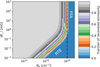 |
Fig. 7 Fraction of modeled synchrotron emissivity of protostars recovered after accounting for SSA, FFA, and the RTE. The fractional emissivity at 144 MHz is shown as a function of ⟨B⊥⟩ and Ne. The temperature of the ionized gas causing FFA is considered to be 104 K. The extinction processes are averaged within 0.03 pc from the modeled protostar, or the LOFAR FWHM at the distance of Perseus. A vertical dash-dotted black line marks the estimated Ne value for our protostellar core sample. |
4.2 Upper limits on the magnetic field in prestellar cores
Recent constraints on the CRe energy spectrum, je, from the Voyager spacecraft (Cummings et al. 2016), have highlighted the impact that GeV-range CRe may have on the synchrotron emission from prestellar cores in molecular clouds (Dickinson et al. 2015; Padovani & Galli 2018). According to Padovani & Galli (2018), for typical magnetic field strengths in prestellar cores (10 μG–1 mG), meter-wavelength synchrotron emission is expected to be observable without significant attenuation below NH2 values of approximately 6 × 1024 cm−2, which is much higher than the typical column densities of prestellar cores. In Sect. 3, we attempted to statistically detect the emission from prestellar cores using LOFAR. However, as is discussed in Sect. 3.3, we did not find any significant counterparts in the corresponding residual stacked maps. Since prestellar cores are defined as starless cores, we cannot explain the lack of detection in terms of extinction of internal radio sources (e.g., jets, shocks), as we did for protostellar cores.
To further investigate the missing radio emission in prestellar cores, we produced synthetic data of Stokes I at 144 MHz. For the magnetic-field structure, we used the 3D axisymmetric models of starless cores of Li & Shu (1996) that were later extended by Galli et al. (1999). These models, which were also employed in Padovani & Galli (2011) and Padovani et al. (2013), describe magnetostatic, isothermal, self-gravitating, axially symmetric cloud cores supported by ordered hourglass magnetic fields3. They are characterized by two main parameters: the effective sound speed, cs,eff, which accounts for both thermal and turbulent support to gravity; and the value of the dimensionless mass-to-flux ratio λr, defined as
![Mathematical equation: $\[\lambda_{r}=2 \pi G^{1 / 2} \frac{M(\Phi)}{\Phi},\]$](/articles/aa/full_html/2025/02/aa52010-24/aa52010-24-eq9.png) (5)
(5)
where G is the gravitational constant, and M(Φ) the mass enclosed in a sphere tangent to the flux tube, Φ.
Given a value of λr, the corresponding magnetic support to gravitational collapse is H0 = ϕ(π/2)λr − 1, where ϕ(π/2) is a dimensionless quantity. We modeled prestellar cores within boxes of approximately (0.6 pc)3, which projected in 2D roughly corresponds to the size of the cutouts used for stacking at the distance of Perseus. As an example, in Fig. 8 we show one 3D rendering of the model with cs,eff = 0.2 km s−1 and λr = 1.52. The strength of the magnetic field varies from a few μJG to more than 200 μJG in the central region within 0.1 pc, as is indicated by the black circle.
Assuming a uniform spatial distribution for the CRe, we estimated ϵν as before, considering two shapes of je from Bracco et al. (2024) and Padovani et al. (2018) to quantify the uncertainties on the CRe assumptions. By convolving the synthetic synchrotron emission with the LOFAR FWHM, we estimated the average Stokes I expected within 0.1 pc from the core for a grid of models defined by realistic values for prestellar cores of cs,eff ∈ [0.17, 0.5] km s−1 and λr ∈ [1.44, 2] (e.g., Crutcher 2012). We integrated the modeled cubes along two orthogonal orientations, θ, along and across the poloidal axis of the magnetic field (z and y directions, respectively, in Fig. 8).
The results of our modeling are shown in Fig. 9. Regions above 5 μJy beam−1, or the 84th percentile of the prestellarcore NDF (see Fig. 6), are indicated with diagonal black hatches. In the right column, we show the mean magnetic-field strength within 0.1 pc for each model.
We note that our statistical analysis of the LOFAR data excludes prestellar-core models with magnetic-field strengths strictly larger than 150 μJG for both je and θ cases. Nevertheless, below the LOFAR noise level, we identified a plausible range of prestellar-core models that could be detected at higher sensitivity with ordered magnetic-field strengths of 100 μG, or less, and with values of cs,eff close to 0.2 km s−1, which corresponds to the sound speed of isothermal cores with a temperature of 10 K.
Despite the simplicity of our model, we reach constraints that are compatible with the very small amount of observational evidence for magnetic-field strengths in prestellar cores, ranging from tens to hundreds of μJG (e.g., Pattle et al. 2023, and references therein). We also notice that most of these observational estimates only represent upper limits on the magnetic-field strength as they rely on the standard Davis-Chandrasekhar-Fermi method applied to interstellar dust polarization measurements, which can statistically overestimate the interstellar magne-tic-field strength by up to an order of magnitude (e.g., Skalidis et al. 2021).
Prestellar cores with magnetic-field strengths below 100 μJG will be observable, and likely detected, with SKA-Low. We used the SKA-Low sensitivity calculator and time estimator4 (Sokolowski et al. 2022), to investigate how many hours would be needed to reach a sensitivity of 2 μJy beam−1 in the residual stacking of the sample of 348 prestellar cores in Perseus at 144 MHz under observational conditions similar to those in LoTSS. In the left and central panels of Fig. 9, we show the 2 μJy beam−1 level with a dashed white line, which should be attainable in only 9 hours and 4 hours of observing time, during the preliminary stage of array assembly5, AA*, and the final stage, AA4, respectively.
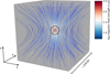 |
Fig. 8 Representation of the magnetic-field structure and strength (in colours) of one of the prestellar-core models from Li & Shu (1996). These models are for isothermal cores at magnetostatic equilibrium. The example is shown for λr = 1.52. The black circle in the middle, with a diameter of ~0.1 pc, indicates the region used to average the magnetic-field strength. The 3D rendering was made with the ParaView software (http://www.paraview.org). |
 |
Fig. 9 Estimated Stokes I at 144 MHz from a grid of prestellar-core models – see one example in Fig. 8 – as a function of the magnetic support (H0) and the effective sound speed in the medium (cs,eff). The corresponding mass-to-flux ratio (λr) is also displayed on the top of each panel. In the left and central panels, two different emissivity models are considered (Padovani et al. 2018; Bracco et al. 2024). In the right panels, for each pair of parameters (cs,eff, H0), we show the corresponding magnetic-field strength averaged within 0.1 pc from the center. In the two rows we integrate the models either edge-on (top) or face-on (bottom). Black hatches define the non-detection areas in the LOFAR data for Stokes I values greater than 5 μJy beam−1. The dashed white lines at 2 μJy beam−1 indicate the sensitivity in Perseus of SKA-Low for ~9 hours of observations in stage AA* and ~4 hours in stage AA4. |
5 Summary and conclusion
Cosmic rays are considered an essential ingredient in the star formation process, determining the ionization rate of molecular gas and its interaction with magnetic fields (e.g., Padovani et al. 2020). The electronic GeV component (CRe) is expected to produce mostly nonthermal synchrotron radiation when interacting with the interstellar magnetic field. Moreover, star formation, protostellar activity, and jets are also thought to locally accelerate CRe in shocks (Padovani et al. 2015, 2016; Gaches & Offner 2018; Padovani et al. 2021b). Despite these theoretical expectations, however, nonthermal emission from molecular clouds in the Milky Way has been observed in only a few cases, such as diffuse emission in the Orion-Taurus ridge (Bracco et al. 2023) and compact regions around one protostellar jet in DG Tau A (Feeney-Johansson et al. 2019).
While nonthermal radiation in the GHz range can be strongly contaminated by thermal free-free emission (e.g., Tobin et al. 2016), the low-frequency range in the radio represents the most promising observational window in which to detect synchrotron emission from molecular clouds (e.g., Dickinson et al. 2015). Although current facilities do not easily achieve the required sensitivity to detect emission from single objects (Padovani & Galli 2018), in this work, we have conducted the first statistical analysis aimed at extracting nonthermal radio emission from hundreds of stellar embryos, both prestellar and protostellar cores, by stacking LOFAR data at 144 MHz from LoTSS (Shimwell et al. 2022) toward the Perseus molecular cloud.
Among the 353 prestellar cores and 132 protostellar cores identified in Perseus by P21 using Herschel data, we found 5 prestellar cores and 18 protostellar cores with significant excess emission in LOFAR data. However, for all these cores, we estimate that the correspondence between far-infrared and radio emissions is likely due to extragalactic contaminations in the Herschel catalog by P21 (see Sects. 3.1 and 3.2). By stacking the remaining prestellar and protostellar cores separately, we could not detect any significant excess in LOFAR at the levels of 5 and 8 μJy beam−1 for prestellar cores and protostellar cores, respectively (see Sect. 3.3). We interpret these results in two ways: in the case of protostellar cores, we propose that the radio emission could be completely extinguished by either FFA or the RTE along the sight line (see Sect. 4.1); in the case of prestellar cores, we conclud that, even after stacking, we are primarily limited by the sensitivity of LoTSS. We compared the observational results with synthetic data from the 3D analytical models of magnetostatic-isothermal cores by Li & Shu (1996) and set upper limits on the ordered magnetic-field strength of prestellar cores to be detected in the stacking of LOFAR data. Statistically, prestellar cores in Perseus should have magnetic-field strengths below 100 μJG within 0.1 pc of the core center (see Sect. 4.2). Using the SKA sensitivity calculator, we predict that such prestellar cores in Perseus will be statistically detectable by SKA-Low in 9 and 4 hours observing time, using the array assemblies AA* and AA4, respectively.
Acknowledgements
We acknowledge the referee’s thorough and insightful comments, which have significantly improved the clarity and content of this manuscript. We are grateful to Tim Shimwell, Florent Mertens, Philippe Zarka, Giulia Macario, Francesca Bacciotti and Marta Fatović for useful discussions. We thank Philippe André for providing us with the column-density map of the Perseus cloud. AB and DG acknowledge financial support from the INAF initiative “IAF Astronomy Fellowships in Italy” (grant name MEGASKAT) and the INAF minigrant PACIFISM, respectively. We also acknowledge the inspiration provided by Delphine and Elio. AD acknowledges support by the BMBF Verbundforschung under the grant 05A20STA. The Jülich LOFAR Long Term Archive and the German LOFAR network are both coordinated and operated by the Jülich Supercomputing Centre (JSC), and computing resources on the supercomputer JUWELS at JSC were provided by the Gauss Centre for Supercomputing e.V. (grant CHTB00) through the John von Neumann Institute for Computing (NIC). LOFAR data products were provided by the LOFAR Surveys Key Science project (LSKSP; https://lofar-surveys.org/) and were derived from observations with the International LOFAR Telescope (ILT). LOFAR (van Haarlem et al. 2013) is the Low Frequency Array designed and constructed by ASTRON. It has observing, data processing, and data storage facilities in several countries, that are owned by various parties (each with their own funding sources), and that are collectively operated by the ILT foundation under a joint scientific policy. The efforts of the LSKSP have benefited from funding from the European Research Council, NOVA, NWO, CNRS-INSU, the SURF Co-operative, the UK Science and Technology Funding Council and the Jülich Supercomputing Centre. In the analysis we made use of astropy (Astropy Collaboration 2018), scipy (Virtanen et al. 2020), and numpy (Harris et al. 2020). This research has made use of “Aladin sky atlas” developed at CDS, Strasbourg Observatory, France.
Appendix A Mosaic of five fields of view from LoTSS
In this study, we combined five single-night 8-hour pointings from the LOFAR internal data release, referred to as P 051+31, P 052+29, P 054+31, P 057+31, and P057+34. Once prepared for publication (Shimwell et al., in prep.), the data will be accessible through the LoTSS repository6. The mosaic was constructed in both Stokes I and Stokes V (see Fig. 2). As an example, in Fig. A.1 we show the two Stokes parameter maps for one single pointing, specifically P054+31. Both maps share the same coordinate grid and projection as the NH2 map shown in Fig. 1.
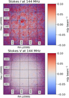 |
Fig. A.1 Stokes I and V maps of Perseus corresponding to the single 8 h pointing P054+31. |
The single-night pointing maps reveal that noise – as traced by Stokes V – is highly non uniform across the field of view, presenting challenges for our stacking analysis. The increased noise at the edges of the image is caused by LOFAR’s primarybeam sensitivity. In the top panel of Fig. A.2, we show the primary-beam weighting of LOFAR with a 3-deg radius, rpb, in white-dashed contour. Beyond rpb, sensitivity drops rapidly. We combined all five pointings, including only the corresponding circular area, ![Mathematical equation: $\[\pi r_{\mathrm{pb}}^{2}\]$](/articles/aa/full_html/2025/02/aa52010-24/aa52010-24-eq10.png) . The overlap of these pointings is illustrated in the bottom panel of Fig. A.2.
. The overlap of these pointings is illustrated in the bottom panel of Fig. A.2.
The quantitative advantage of the mosaic with respect to single pointing observations is seen in the noise levels in Fig. A.3. Since the Perseus molecular cloud has an elongated RA extent (see Fig. 1), we present the RMS value of Stokes V as a function of RA for NH2 > 1021 cm−2, where most of our core samples are located (see Fig. 1). For a single pointing (P054+31), the RMS varies by more than a factor of five (black line), while in the mosaic, it remains stable between 0.1 and 0.2 mJy beam−1 (magenta line).
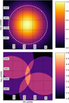 |
Fig. A.2 LOFAR primary-beam weighting (top panel) and overlap of the five pointings used for the mosaic (bottom panel). A white-dashed circle of 3-deg radius in the top panel defines the region in each pointing utilised to produce the mosaic. |
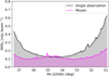 |
Fig. A.3 Root mean square of Stokes V as a function of RA for the P054+31 pointing (in black) for NH2 > 1021 cm−2 (see Fig. 1). The single-night RMS is compared to the RMS of the mosaic shown in magenta. |
Appendix B Cutout maps of the bright cores in LOFAR
In this Appendix we show the cutouts of each selected bright core in the LOFAR data, as described in Sect. 3.1. In Figs. B.1 and B.2, the corresponding images of protostellar and prestellar cores are displayed.
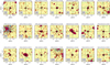 |
Fig. B.1 Stokes-I cutouts around each protostar selected in Fig. 4. The corresponding source name as in P21 and index are displayed in gray. The color-range for all sources is between −1 and 1 mJy beam−1. |
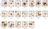 |
Fig. B.2 Same as in Fig. B.1 but for prestellar cores using the same dynamic range between −1 and 1 mJy beam−1. |
References
- Andre, P., Ward-Thompson, D., & Barsony, M. 2000, in Protostars and Planets IV, eds. V. Mannings, A. P. Boss, & S. S. Russell, 59 [Google Scholar]
- André, P., Men’shchikov, A., Bontemps, S., et al. 2010, A&A, 518, L102 [NASA ADS] [CrossRef] [EDP Sciences] [Google Scholar]
- Anglada, G. 1995, in Revista Mexicana de Astronomia y Astrofisica Conference Series, 1, Revista Mexicana de Astronomia y Astrofisica Conference Series, eds. S. Lizano, & J. M. Torrelles, 67 [Google Scholar]
- Astropy Collaboration (Price-Whelan, A. M., et al.) 2018, AJ, 156, 123 [Google Scholar]
- Ballesteros-Paredes, J., André, P., Hennebelle, P., et al. 2020, Space Sci. Rev., 216, 76 [Google Scholar]
- Boch, T., & Fernique, P. 2014, in Astronomical Society of the Pacific Conference Series, 485, Astronomical Data Analysis Software and Systems XXIII, eds. N. Manset. & P. Forshay, 277 [Google Scholar]
- Bracco, A., Palmeirim, P., André, P., et al. 2017, A&A, 604, A52 [NASA ADS] [CrossRef] [EDP Sciences] [Google Scholar]
- Bracco, A., Bresnahan, D., Palmeirim, P., et al. 2020, A&A, 644, A5 [NASA ADS] [CrossRef] [EDP Sciences] [Google Scholar]
- Bracco, A., Padovani, M., & Soler, J. D. 2023, A&A, 677, L11 [NASA ADS] [CrossRef] [EDP Sciences] [Google Scholar]
- Bracco, A., Padovani, M., & Galli, D. 2024, A&A, 686, A52 [NASA ADS] [CrossRef] [EDP Sciences] [Google Scholar]
- Chen, T. X., Ebert, R., Mazzarella, J. M., et al. 2022, PASP, 134, 014501 [NASA ADS] [CrossRef] [Google Scholar]
- Condon, J. J., Cotton, W. D., Greisen, E. W., et al. 1998, AJ, 115, 1693 [Google Scholar]
- Coudé, S., Bastien, P., Houde, M., et al. 2019, ApJ, 877, 88 [Google Scholar]
- Coughlan, C. P., Ainsworth, R. E., Eislöffel, J., et al. 2017, ApJ, 834, 206 [Google Scholar]
- Crutcher, R. M. 2012, ARA&A, 50, 29 [Google Scholar]
- Crutcher, R. M., Wandelt, B., Heiles, C., Falgarone, E., & Troland, T. H. 2010, ApJ, 725, 466 [NASA ADS] [CrossRef] [Google Scholar]
- Cummings, A. C., Stone, E. C., Heikkila, B. C., et al. 2016, ApJ, 831, 18 [CrossRef] [Google Scholar]
- de Gasperin, F., Dijkema, T. J., Drabent, A., et al. 2019, A&A, 622, A5 [NASA ADS] [CrossRef] [EDP Sciences] [Google Scholar]
- Dewdney, P. E., Hall, P. J., Schilizzi, R. T., & Lazio, T. J. L. W. 2009, IEEE Proc., 97, 1482 [Google Scholar]
- Dickinson, C., Beck, R., Crocker, R., et al. 2015, in Advancing Astrophysics with the Square Kilometre Array (AASKA14), 102 [CrossRef] [Google Scholar]
- Doi, Y., Hasegawa, T., Bastien, P., et al. 2021, ApJ, 914, 122 [NASA ADS] [CrossRef] [Google Scholar]
- Drabent, A., Hoeft, M., Mechev, A. P., et al. 2019, arXiv e-prints [arXiv:1910.13835] [Google Scholar]
- Dunham, M. M., Crapsi, A., Evans, Neal J., I., et al. 2008, ApJS, 179, 249 [NASA ADS] [CrossRef] [Google Scholar]
- Evans, Neal J., I., Dunham, M. M., Jørgensen, J. K., et al. 2009, ApJS, 181, 321 [NASA ADS] [CrossRef] [Google Scholar]
- Fedriani, R., Caratti o Garatti, A., Purser, S. J. D., et al. 2019, Nat. Commun., 10, 3630 [NASA ADS] [CrossRef] [Google Scholar]
- Feeney-Johansson, A., Purser, S. J. D., Ray, T. P., et al. 2019, ApJ, 885, L7 [Google Scholar]
- Gabici, S. 2022, A&A Rev., 30, 4 [NASA ADS] [CrossRef] [Google Scholar]
- Gaches, B. A. L., & Offner, S. S. R. 2018, ApJ, 861, 87 [NASA ADS] [CrossRef] [Google Scholar]
- Galli, D., Lizano, S., Li, Z. Y., Adams, F. C., & Shu, F. H. 1999, ApJ, 521, 630 [Google Scholar]
- Ginzburg, V. L., & Syrovatskii, S. I. 1965, ARA&A, 3, 297 [Google Scholar]
- Girart, J. M., Rao, R., & Marrone, D. P. 2006, Science, 313, 812 [Google Scholar]
- Grenier, I. A., Black, J. H., & Strong, A. W. 2015, ARA&A, 53, 199 [Google Scholar]
- Hacar, A., Clark, S. E., Heitsch, F., et al. 2023, in Astronomical Society of the Pacific Conference Series, 534, Protostars and Planets VII, eds. S. Inutsuka, Y. Aikawa, T. Muto, K. Tomida, & M. Tamura, 153 [Google Scholar]
- Harris, C. R., Millman, K. J., van der Walt, S. J., et al. 2020, Nature, 585, 357 [NASA ADS] [CrossRef] [Google Scholar]
- Heiles, C., & Troland, T. H. 2003, ApJ, 586, 1067 [NASA ADS] [CrossRef] [Google Scholar]
- Hennebelle, P., & Inutsuka, S.-i. 2019, Front. Astron. Space Sci., 6, 5 [Google Scholar]
- Intema, H. T., Jagannathan, P., Mooley, K. P., & Frail, D. A. 2017, A&A, 598, A78 [NASA ADS] [CrossRef] [EDP Sciences] [Google Scholar]
- Ivlev, A. V., Silsbee, K., Padovani, M., & Galli, D. 2021, ApJ, 909, 107 [NASA ADS] [CrossRef] [Google Scholar]
- Lee, N., Le Floc’h, E., Sanders, D. B., et al. 2010, ApJ, 717, 175 [Google Scholar]
- Li, Z.-Y., & Shu, F. H. 1996, ApJ, 472, 211 [NASA ADS] [CrossRef] [Google Scholar]
- Magnier, E. A., Schlafly, E. F., Finkbeiner, D. P., et al. 2020, ApJS, 251, 6 [NASA ADS] [CrossRef] [Google Scholar]
- Maury, A., Hennebelle, P., & Girart, J. M. 2022, Front. Astron. Space Sci., 9, 949223 [NASA ADS] [CrossRef] [Google Scholar]
- Momferratos, G., Lesaffre, P., Falgarone, E., & Pineau des Forêts, G. 2014, MNRAS, 443, 86 [NASA ADS] [CrossRef] [Google Scholar]
- Offringa, A. R., van de Gronde, J. J., & Roerdink, J. B. T. M. 2012, A&A, 539, A95 [NASA ADS] [CrossRef] [EDP Sciences] [Google Scholar]
- Padovani, M., & Galli, D. 2011, A&A, 530, A109 [NASA ADS] [CrossRef] [EDP Sciences] [Google Scholar]
- Padovani, M., & Galli, D. 2018, A&A, 620, L4 [NASA ADS] [CrossRef] [EDP Sciences] [Google Scholar]
- Padovani, M., Hennebelle, P., & Galli, D. 2013, A&A, 560, A114 [NASA ADS] [CrossRef] [EDP Sciences] [Google Scholar]
- Padovani, M., Hennebelle, P., Marcowith, A., & Ferrière, K. 2015, A&A, 582, L13 [NASA ADS] [CrossRef] [EDP Sciences] [Google Scholar]
- Padovani, M., Marcowith, A., Hennebelle, P., & Ferrière, K. 2016, A&A, 590, A8 [NASA ADS] [CrossRef] [EDP Sciences] [Google Scholar]
- Padovani, M., Galli, D., Ivlev, A. V., Caselli, P., & Ferrara, A. 2018, A&A, 619, A144 [NASA ADS] [CrossRef] [EDP Sciences] [Google Scholar]
- Padovani, M., Ivlev, A. V., Galli, D., et al. 2020, Space Sci. Rev., 216, 29 [CrossRef] [Google Scholar]
- Padovani, M., Bracco, A., Jelić, V., Galli, D., & Bellomi, E. 2021a, A&A, 651, A116 [NASA ADS] [CrossRef] [EDP Sciences] [Google Scholar]
- Padovani, M., Marcowith, A., Galli, D., Hunt, L. K., & Fontani, F. 2021b, A&A, 649, A149 [NASA ADS] [CrossRef] [EDP Sciences] [Google Scholar]
- Padovani, M., Bialy, S., Galli, D., et al. 2022, A&A, 658, A189 [NASA ADS] [CrossRef] [EDP Sciences] [Google Scholar]
- Pattle, K., Fissel, L., Tahani, M., Liu, T., & Ntormousi, E. 2023, in Astronomical Society of the Pacific Conference Series, 534, Protostars and Planets VII, eds. S. Inutsuka, Y. Aikawa, T. Muto, K. Tomida, & M. Tamura, 193 [Google Scholar]
- Pezzuto, S., Benedettini, M., Di Francesco, J., et al. 2021, A&A, 645, A55 [EDP Sciences] [Google Scholar]
- Pilbratt, G. L., Riedinger, J. R., Passvogel, T., et al. 2010, A&A, 518, L1 [NASA ADS] [CrossRef] [EDP Sciences] [Google Scholar]
- Pinto, C., Galli, D., & Bacciotti, F. 2008, A&A, 484, 1 [NASA ADS] [CrossRef] [EDP Sciences] [Google Scholar]
- Planck Collaboration I. 2016, A&A, 594, A1 [NASA ADS] [CrossRef] [EDP Sciences] [Google Scholar]
- Planck Collaboration Int. XXXII. 2016, A&A, 586, A135 [NASA ADS] [CrossRef] [EDP Sciences] [Google Scholar]
- Planck Collaboration Int. XXXV. 2016, A&A, 586, A138 [NASA ADS] [CrossRef] [EDP Sciences] [Google Scholar]
- Purser, S. J. D., Ainsworth, R. E., Ray, T. P., et al. 2018, MNRAS, 481, 5532 [NASA ADS] [CrossRef] [Google Scholar]
- Rodríguez-Kamenetzky, A., Carrasco-González, C., Araudo, A., et al. 2016, ApJ, 818, 27 [CrossRef] [Google Scholar]
- Rodríguez-Kamenetzky, A., Carrasco-González, C., Araudo, A., et al. 2017, ApJ, 851, 16 [Google Scholar]
- Sanna, A., Moscadelli, L., Goddi, C., et al. 2019, A&A, 623, L3 [NASA ADS] [CrossRef] [EDP Sciences] [Google Scholar]
- Scaife, A. M. M., & Heald, G. H. 2012, MNRAS, 423, L30 [Google Scholar]
- Shimwell, T. W., Röttgering, H. J. A., Best, P. N., et al. 2017, A&A, 598, A104 [NASA ADS] [CrossRef] [EDP Sciences] [Google Scholar]
- Shimwell, T. W., Tasse, C., Hardcastle, M. J., et al. 2019, A&A, 622, A1 [NASA ADS] [CrossRef] [EDP Sciences] [Google Scholar]
- Shimwell, T. W., Hardcastle, M. J., Tasse, C., et al. 2022, A&A, 659, A1 [NASA ADS] [CrossRef] [EDP Sciences] [Google Scholar]
- Skalidis, R., Sternberg, J., Beattie, J. R., Pavlidou, V., & Tassis, K. 2021, A&A, 656, A118 [NASA ADS] [CrossRef] [EDP Sciences] [Google Scholar]
- Skrutskie, M. F., Cutri, R. M., Stiening, R., et al. 2006, AJ, 131, 1163 [NASA ADS] [CrossRef] [Google Scholar]
- Smirnov, O. M., & Tasse, C. 2015, MNRAS, 449, 2668 [Google Scholar]
- Sokolowski, M., Tingay, S. J., Davidson, D. B., et al. 2022, PASA, 39, e015 [NASA ADS] [CrossRef] [Google Scholar]
- Soler, J. D. 2019, A&A, 629, A96 [NASA ADS] [CrossRef] [EDP Sciences] [Google Scholar]
- Stanislavsky, L. A., Bubnov, I. N., Konovalenko, A. A., Stanislavsky, A. A., & Yerin, S. N. 2023, A&A, 670, A157 [NASA ADS] [CrossRef] [EDP Sciences] [Google Scholar]
- Tasse, C. 2014, A&A, 566, A127 [NASA ADS] [CrossRef] [EDP Sciences] [Google Scholar]
- Tasse, C., Hugo, B., Mirmont, M., et al. 2018, A&A, 611, A87 [NASA ADS] [CrossRef] [EDP Sciences] [Google Scholar]
- Thompson, K. L., Troland, T. H., & Heiles, C. 2019, ApJ, 884, 49 [NASA ADS] [CrossRef] [Google Scholar]
- Tobin, J. J., Looney, L. W., Li, Z.-Y., et al. 2016, ApJ, 818, 73 [CrossRef] [Google Scholar]
- Tychoniec, Ł., Tobin, J. J., Karska, A., et al. 2018, ApJS, 238, 19 [Google Scholar]
- van Diepen, G., Dijkema, T. J., & Offringa, A. 2018, DPPP: Default Pre-Processing Pipeline, Astrophysics Source Code Library [record ascl:1804.003] [Google Scholar]
- van Haarlem, M. P., Wise, M. W., Gunst, A. W., et al. 2013, A&A, 556, A2 [NASA ADS] [CrossRef] [EDP Sciences] [Google Scholar]
- van Weeren, R. J., Williams, W. L., Hardcastle, M. J., et al. 2016, ApJS, 223, 2 [Google Scholar]
- Virtanen, P., Gommers, R., Oliphant, T. E., et al. 2020, Nature Methods, 17, 261 [CrossRef] [Google Scholar]
- Williams, W. L., van Weeren, R. J., Röttgering, H. J. A., et al. 2016, MNRAS, 460, 2385 [Google Scholar]
- Zucker, C., Speagle, J. S., Schlafly, E. F., et al. 2019, ApJ, 879, 125 [NASA ADS] [CrossRef] [Google Scholar]
Our analytical models do not account for any turbulent magnetic-field component.
For more details on the array assembly key information visit, https://www.skao.int/en/science-users/ska-tools/494/ska-staged-delivery-array-assemblies-and-subarrays
All Tables
All Figures
|
Fig. 1 Column density map of molecular hydrogen, NH2, combining Herschel and Planck data of the Perseus molecular cloud. Magenta and cyan circles correspond to protostellar and prestellar cores, respectively, as they are defined in P21. |
| In the text | |
|
Fig. 2 Stokes I and V maps of the Perseus molecular cloud from the LoTSS survey. The maps have the same projection and grid as the NH2 map shown in Fig. 1, centered on the celestial coordinate (RA, Dec) (J2000) = (54°, +31°). |
| In the text | |
|
Fig. 3 Stacked maps of Stokes I (left) and V (right) from LOFAR at 144 MHz for protostellar (top) and prestellar (bottom) cores in the Perseus molecular cloud. The synthetized beam of 20″ FWHM is shown with a white circle in the top left panel. The central region where the mean stacking is performed is shown in all panels by the black circle at the center, which is twice the size of the FWHM. At the distance of Perseus (~300 pc), 90″ corresponds to ~0.15 pc. |
| In the text | |
|
Fig. 4 Ratio (ℛ) between the mean of Stokes I within the central region (black circle in Fig. 3) and the RMS value of Stokes V in the outer region (see top panels), for prestellar (right) and protostellar (left) cores. ℛ is shown as a function of the RA coordinate of each core. The selected sources correspond to ℛ values greater than 2 (black dots above the dashed blue line) and 3 (red dots above the dashed red line). |
| In the text | |
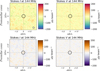 |
Fig. 5 Residual stacked maps without the selected sources shown in Figs. 4, B.1, and B.2. |
| In the text | |
|
Fig. 6 Normalized distribution functions for protostellar (left) and prestellar (right) cores of the residual stacked Stokes-I (blue) and -V (purple) maps averaged within 5000 circles of equal area as the central black circle in Figs. 3 and 5. The measured values at the center are shown with diagonal black hatches depending on the choice of ℛ for defining the outlier cores. From dark to light colours, shadows correspond to 1-, 2-, and 3-σ levels. The 84 th percentiles are 8 μJy beam−1 and 5 μJy beam−1 for protostellar and prestellar cores, respectively. The NDF are shown with both histograms and kernel density estimates. |
| In the text | |
|
Fig. 7 Fraction of modeled synchrotron emissivity of protostars recovered after accounting for SSA, FFA, and the RTE. The fractional emissivity at 144 MHz is shown as a function of ⟨B⊥⟩ and Ne. The temperature of the ionized gas causing FFA is considered to be 104 K. The extinction processes are averaged within 0.03 pc from the modeled protostar, or the LOFAR FWHM at the distance of Perseus. A vertical dash-dotted black line marks the estimated Ne value for our protostellar core sample. |
| In the text | |
|
Fig. 8 Representation of the magnetic-field structure and strength (in colours) of one of the prestellar-core models from Li & Shu (1996). These models are for isothermal cores at magnetostatic equilibrium. The example is shown for λr = 1.52. The black circle in the middle, with a diameter of ~0.1 pc, indicates the region used to average the magnetic-field strength. The 3D rendering was made with the ParaView software (http://www.paraview.org). |
| In the text | |
|
Fig. 9 Estimated Stokes I at 144 MHz from a grid of prestellar-core models – see one example in Fig. 8 – as a function of the magnetic support (H0) and the effective sound speed in the medium (cs,eff). The corresponding mass-to-flux ratio (λr) is also displayed on the top of each panel. In the left and central panels, two different emissivity models are considered (Padovani et al. 2018; Bracco et al. 2024). In the right panels, for each pair of parameters (cs,eff, H0), we show the corresponding magnetic-field strength averaged within 0.1 pc from the center. In the two rows we integrate the models either edge-on (top) or face-on (bottom). Black hatches define the non-detection areas in the LOFAR data for Stokes I values greater than 5 μJy beam−1. The dashed white lines at 2 μJy beam−1 indicate the sensitivity in Perseus of SKA-Low for ~9 hours of observations in stage AA* and ~4 hours in stage AA4. |
| In the text | |
|
Fig. A.1 Stokes I and V maps of Perseus corresponding to the single 8 h pointing P054+31. |
| In the text | |
|
Fig. A.2 LOFAR primary-beam weighting (top panel) and overlap of the five pointings used for the mosaic (bottom panel). A white-dashed circle of 3-deg radius in the top panel defines the region in each pointing utilised to produce the mosaic. |
| In the text | |
|
Fig. A.3 Root mean square of Stokes V as a function of RA for the P054+31 pointing (in black) for NH2 > 1021 cm−2 (see Fig. 1). The single-night RMS is compared to the RMS of the mosaic shown in magenta. |
| In the text | |
|
Fig. B.1 Stokes-I cutouts around each protostar selected in Fig. 4. The corresponding source name as in P21 and index are displayed in gray. The color-range for all sources is between −1 and 1 mJy beam−1. |
| In the text | |
|
Fig. B.2 Same as in Fig. B.1 but for prestellar cores using the same dynamic range between −1 and 1 mJy beam−1. |
| In the text | |
Current usage metrics show cumulative count of Article Views (full-text article views including HTML views, PDF and ePub downloads, according to the available data) and Abstracts Views on Vision4Press platform.
Data correspond to usage on the plateform after 2015. The current usage metrics is available 48-96 hours after online publication and is updated daily on week days.
Initial download of the metrics may take a while.