| Issue |
A&A
Volume 694, February 2025
|
|
|---|---|---|
| Article Number | A233 | |
| Number of page(s) | 16 | |
| Section | Planets, planetary systems, and small bodies | |
| DOI | https://doi.org/10.1051/0004-6361/202451994 | |
| Published online | 18 February 2025 | |
Characterising WASP-43b’s interior structure: Unveiling tidal decay and apsidal motion
1
Institute of Planetary Research, German Aerospace Center (DLR),
Rutherfordstrasse 2,
12489
Berlin,
Germany
2
ELKH-SZTE Stellar Astrophysics Research Group,
6500
Baja,
Szegedi út Kt. 766,
Hungary
3
Konkoly Observatory, Research Centre for Astronomy and Earth Sciences, HUN-REN, MTA Centre of Excellence,
Konkoly-Thege Miklós út 15–17.,
1121,
Hungary
4
HUN-REN-ELTE Exoplanet Research Group,
Szombathely,
Szent Imre h. u. 112.,
9700,
Hungary
5
ELTE Eötvös Loránd University, Doctoral School of Physics,
Budapest,
Pázmány Péter sétány 1/A,
1117,
Hungary
6
Institut für Geologische Wissenschaften, Freie Universität Berlin,
12249
Berlin,
Germany
7
Dipartimento di Fisica, Università degli Studi di Torino,
Via Pietro Giuria, 1,
10125
Torino,
Italy
8
INAF – Osservatorio Astrofisico di Arcetri,
Largo Enrico Fermi 5,
50125
Firenze,
Italy
9
Observatoire Astronomique de l’Université de Genève,
Chemin Pegasi 51,
1290
Versoix,
Switzerland
10
Centre Vie dans l’Univers, Faculté des sciences, Université de Genève,
Quai Ernest-Ansermet 30,
1211
Genève 4,
Switzerland
11
Thüringer Landessternwarte Tautenburg,
Sternwarte 5,
07778
Tautenburg,
Germany
★ Corresponding author; This email address is being protected from spambots. You need JavaScript enabled to view it.
; This email address is being protected from spambots. You need JavaScript enabled to view it.
Received:
26
August
2024
Accepted:
3
January
2025
Abstract
Context. Recent developments in exoplanetary research highlight the importance of Love numbers in understanding the internal dynamics, formation, migration history, and potential habitability of exoplanets. Love numbers represent crucial parameters that gauge how exoplanets respond to external forces such as tidal interactions and rotational effects. By measuring these responses, insights into the internal structure, composition, and density distribution of exoplanets can be gained. The rate of apsidal precession of a planetary orbit is directly linked to the second-order fluid Love numbers. Thus, Love numbers can also offer valuable insights into the mass distribution of a planet.
Aims. In this context, we aim to re-determine the orbital parameters of WASP-43b – in particular, the orbital period, eccentricity, and argument of the periastron – and its orbital evolution. We study the outcomes of the tidal interaction with the host star in order to identify whether tidal decay and periastron precession occur in the system.
Methods. We observed WASP-43b with HARPS, whose data we present for the first time, and we also analysed the newly acquired JWST full-phase light curve. We jointly fit new and archival radial velocity and transit and occultation mid-times, including tidal decay, periastron precession, and long-term acceleration in the system.
Results. We detected a tidal decay rate of Ṗa = (−l.99±0.50) ms yr−1 and a periastron precession rate of ω = 0.1727−0.0089+0.0083)° d−1 = (621.72−32.04+29.88)″ d−1). This is the first time that both periastron precession and tidal decay are simultaneously detected in an exoplanetary system. The observed tidal interactions can neither be explained by the tidal contribution to apsidal motion of a non-aligned stellar or planetary rotation axis nor by assuming a non-synchronous rotation for the planet, and a value for the planetary Love number cannot be derived. Moreover, we excluded the presence of a second body (e.g. a distant companion star or a yet undiscovered planet) down to a planetary mass of ≳0.3 MJ and up to an orbital period of ≲3700 days. We leave the question of the cause of the observed apsidal motion open.
Key words: planets and satellites: dynamical evolution and stability / planets and satellites: gaseous planets / planets and satellites: interiors / planet–star interactions
© The Authors 2025
 Open Access article, published by EDP Sciences, under the terms of the Creative Commons Attribution License (https://creativecommons.org/licenses/by/4.0), which permits unrestricted use, distribution, and reproduction in any medium, provided the original work is properly cited.
This article is published in open access under the Subscribe to Open model. This email address is being protected from spambots. You need JavaScript enabled to view it. to support open access publication.
1 Introduction
Among the abundance of exoplanets confirmed thus far, hot Jupiters – characterised by their high mass, size, and proximity to their host stars – inhabit the most extreme environments. These characteristics generate large transit and radial velocity signals, and they contribute to the precise determination of various planetary system parameters, including planetary mass, radius, surface gravity, orbital distance, and stellar density. The identification of such planetary characteristics has significantly advanced theoretical comprehension of these systems, which may deviate from the architectural norm observed in the Solar System, and has allowed for the exploration of planetary composition and internal structure, offering valuable insights into the formation, evolution, and migration history of these planets. Tidal forces play a crucial role in this context, as they influence the variety and composition of these systems (see, e.g., Valencia et al. 2006; Sotin et al. 2007; Hatzes & Rauer 2015). Moreover, investigation of tidal interactions between a star and a hot Jupiter has unveiled insights into the internal structures of celestial bodies. Despite the observational advantages, such as the large signal-to-noise ratio, the origin of hot Jupiters is still unclear (see for example Dawson & Johnson 2018).
The knowledge of the mass and radius of an exoplanet – and consequently its bulk density – plays a crucial role in categorising it as a rocky planet or a hot gaseous Jupiter-like body, for example. However, this information alone is insufficient to unveil their internal structure, encompassing layers, thickness, and composition (see, e.g., Seager et al. 2007 and references therein). Potential solutions often exhibit high degeneracy and present multiple interior compositions that differ qualitatively but equally match the observed data. In the context of Jupiter-like close-in planets, Love numbers (Love 1911) emerge as valuable information (see, e.g., Becker & Batygin 2013). Specifically, the second-order fluid Love number k2,p is directly proportional to the mass concentration towards the centre of a celestial body. Padovan et al. (2018) and Baumeister et al. (2020) have demonstrated that incorporating this parameter as an input in an interior structure model significantly diminishes the ambiguity associated with potential internal structures.
In this context, WASP-18Ab (Csizmadia et al. 2019) and WASP-19Ab (Bernabò et al. 2024) were previously chosen as case studies. We now include WASP-43b in our investigation. WASP-43b is an ultra-hot Jupiter (with period P < 1 d) with ≃2 M orbiting around a K7V-type star 87 parsecs away, with a period of ≃0.813 d.
While orbital decay has been confirmed in WASP-12b (see Maciejewski et al. 2016; Yee et al. 2020 and references therein), the case of WASP-43b is still under discussion. A detailed description of the literature on WASP-43b’s (non)detections of tidal decay is given in Section 3. WASP-43b is one of the best candidates for observing decay and the general outcomes of tidal interaction between the planet and the host star due to its high planet-to-star mass ratio and proximity to the host star.
This paper follows the approach and method of Bernabò et al. (2024), and we aim to investigate the orbital evolution of WASP- 43b and the planetary Love number. We collected archival transit and occultation data and performed a new radial velocity (RV) study of the system with the High Accuracy Radial velocity Planet Searcher (HARPS). We also analyse for the first time four RV datasets that are public but have never been published previously.
The paper is organised as follows. In Section 2, we present transit and occultation timing observations, previous RV studies, and new HARPS RV data. In Section 3, we fit the RV and transit and occultation mid-times with a model including a long-term acceleration of the system, tidal decay, and apsidal motion in the planetary orbit. In Section 4, we discuss the implications and possible explanations of our findings, such as the non-synchronous rotation of WASP-43b, the presence of a second putative planetary body in the system, and the stellar rotation axis inclination.
2 Data
2.1 Transits and occultations
The mid-transit times used in this paper are listed in Table A.1, and the mid-occultation times are in Table A.2. These data are taken from previously published literature and from the Exoplanet Transit Database (ETD1; Poddaný et al. 2010) and the ExoClock2 (Kokori et al. 2022) database. In these two databases, we discarded data with incomplete transits or low- quality (according to the quality flag assigned by the databases) observations. In case any transit event from such databases was not published yet, the observer was contacted directly to gain permission to use the data. We also analysed a full phase curve taken by the James Webb Space Telescope (JWST; Gardner et al. 2006) on 1 and 2 December 2022 (published in Bell et al. 2024) with the Transit Light Curve Modeller (TLCM; Csizmadia 2020) and unpublished transits from the Transiting Exoplanet Survey Satellite (TESS; Ricker et al. 2016) Sector 62. More details are given in Sections 2.1.1 and 2.1.2.
For each transit and occultation mid-time, the time unit was checked. If necessary, we transformed it into BJDTDB (Barycentric Julian Date in the Barycentric Dynamical Time) with the help of the online conversion tool developed by Eastman et al. (2010)3.
2.1.1 JWST phase curve
We fitted the full-phase light curve acquired by JWST with the MIRI instrument between 6.5 and 7.0 µm. The data were published by Bell et al. (2024), but no study has performed a comprehensive analysis of transit, occultation, and phase curve yet. We used TLCM to retrieve the transit and occultation parameters (Csizmadia 2020). We used limb darkening priors from ExoCTK4, and we fitted the reflection effect (including a shift with respect to the sub-stellar point), red noise, white noise, the intensity ratio, the beaming effect, and the ellipsoidal effect. The correlated noise was handled with a wavelet-based method (Carter & Winn 2009; Csizmadia et al. 2023). The full-phase curve was modelled with a Lambertian fit.
First, we fitted the full-phase curve and then the transit and two occultations separately. The transit and occultation midtimes that resulted from the individual fit of the three events are also reported in Tables A.1 and A.2 and are used in the fit in Section 3. In particular, the two occultations are essential since they come after ≃8 years of no reported mid-occultation time and fundamentally helped us discern the transit timing variation (TTV) trend between tidal decay and apsidal motion (see Section 3.6, Figure 9 and its relative discussion for more details).
In Table 1, we show the value of the fitting parameters, and in Figure 1 we show the best fit of the full phase and its residuals. The transit duration is derived as  hours.
2.1.2 TESS Sector 62
We also included previously unpublished observations of WASP- 43b made by TESS. Sector 62 was observed in February and March 2023 at a 120-second and 20-second cadence. Twentyeight transits of WASP-43b were captured with both exposure times. We analysed them with TLCM, and two mid-transit times were obtained corresponding with the two exposure times. The fitting parameters are reported in Table 2, while in Figure 2 we show the 120s phase-folded transits and their residuals.
2.2 Radial velocities
In this work, we used literature and yet unpublished RV data as well as newly acquired HARPS data. In Table 3, we list details on the datasets, as labelled in the table, while in Table B.1 we report the seven RV datasets, where all times are corrected to BJDTDB. In Table 3, we highlight the number of out-of-transit data points, as these are the ones we use since our model does not fit the Rossiter-McLaughlin (RM) effect. In Section 4.3, we separately fit the RM effect in order to constrain the stellar spin-orbit angle. The datasets are labelled as follows:
- ID 1
Hellier et al. (2011), discovery paper: fifteen radialvelocity measurements between January and July 2010 as a follow-up to the CORALIE spectrograph at the Swiss 1.2-metre Leonhard Euler Telescope at ESO’s La Silla Observatory.
- ID 2
Gillon et al. (2012): eight spectra acquired in February and March 2011 by CORALIE.
- ID 3
This work: sixty-seven unpublished spectra taken in 2012 by HARPS-S (Mayor et al. 2003) to measure the spin-orbit angle via the RM effect and orbital eccentricity. PI: A. Triaud, program ID: 089.C-0151.
- ID 4
Esposito et al. (2017): thirty-two spectra acquired by HARPS-S during and around one transit in 2013 and eight additional spectra later in 2013 and 2015. Twenty-seven of these data points were also published in Bonomo et al. (2017).
- ID 5
This work: twenty-one unpublished HARPS-N (Cosentino et al. 2012) spectra acquired during and around one transit in 2015. Program ID: OPT15B_19.
- ID 6
This work: unpublished spectra taken in 2016 by HARPS- S to resolve the planetary atmosphere with transit spectroscopy. The total number of available RV spectra is actually 101; However, we selected only the first and third night of observations due to the low signal-to-noise ratio of the second night data. PI: D. Ehrenreich, program ID: 096.C-0331.
- ID 7
This work: one hundred twenty-eight unpublished ESPRESSO spectra taken in 2020 to study the escape mechanism of WASP-43b’s atmosphere. PI: L. Pino, program ID: 0102.C-0820.
- ID 8
This work: nineteen newly acquired RV points were taken for this study using HARPS-S. PI: Sz. Csizmadia, program ID: 0104.C-0849.
These RV observations cover a time span of ten years and are plotted in Figure 3, where the offsets among them were subtracted for a clear plot.
Fitting parameters of the JWST light curve.
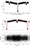 |
Fig. 1 James Webb Space Telescope transit and occultations. Top plot: JWST full-phase observations in time. Middle plot: phase-folded data points in black and best fit in red. To keep the figure clean, error bars are not plotted, but a typical error bar value is shown at the location (0.2,0.98). Grey points are the same as black points but shifted by ±1.0 in phase to make the full phase clearer. Bottom plot: residuals of the fit, after having subtracted the red noise, with a standard deviation of ≃0.00097. |
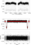 |
Fig. 2 Sector 62 of TESS. Top plot: TESS 120-second full-phase observations in time. Middle plot: phase-folded data points in black and best fit in red. The typical error bar value is shown at the location (0.2,0.98). Grey points are shifted by ±1.0 in phase. The occultation is slightly visible at phase ≃0.5. Bottom plot: residuals of the fit, after having subtracted the red noise, with a standard deviation of ≃0.0017. |
Fitting parameters of TESS light curves.
Radial velocity datasets.
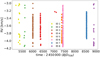 |
Fig. 3 Previously published and new radial velocity observations of WASP-43. The different datasets are plotted with different colours showing the time distribution of the RV observations. |
3 Data analysis
3.1 Eccentricity study
Most close-in planets have been found to be on a circular orbit due to the strong tidal interactions with their host star leading to the quick circularisation of the orbit (see, e.g., Zahn 2008). In the case of WASP-18Ab (Csizmadia et al. 2019) and WASP-19Ab (Bernabò et al. 2024), a long-distance companion star is supposed to be a possible cause of their slightly eccentric orbits (see also Appendix B in Bernabò et al. 2024). A requirement for apsidal motion to take place is that the orbital eccentricity is not zero. Therefore, we analysed the orbital eccentricity as a precondition for our study. Other USP planets are likely in a slightly eccentric orbit. Apart from the two aforementioned cases, the following are examples of USP planets in multi-planetary systems: 55 Cnc e with e = 0.05 ± 0.03, GJ 367b with  (Goffo et al. 2023), TOI-500b with
  (Serrano et al. 2022), and LHS 1678b with
  (Silverstein et al. 2024).
In many studies on WASP-43b, its orbit is assumed to be circular (see for example Hellier et al. 2011; Chen et al. 2014). Through transit, occultation, and RV fitting, Hellier et al. (2011) gave an upper limit of 0.04 at 3σ for the eccentricity and adopted a circular orbit for the fit. Gillon et al. (2012) deduced  and assumed the result to be consistent with a fully circularised orbit. Blecic et al. (2014) found a mid-occultation phase of 0.5001 ± 0.0004 and
  , and Chen et al. (2014) found an offset occultation phase of
  .
.
We used the most complete, up-to-date, and extended RV, transit, and occultation dataset, which includes unpublished data, to determine the orbital eccentricity of WASP-43b. This comprehensive dataset ensures a precise and robust analysis of the planet’s orbital parameters.
We fitted the complete RV, transit, and occultation mid-times dataset with a one-planet circular model and one-planet eccentric model, and we compared the results. Notably, our analysis incorporates a significantly larger dataset than previous studies, as we utilised 471 data points, making it the largest dataset compared to the aforementioned studies. When fitting an eccentric planet, the eccentricity resulted in being significantly different from zero:  , (1σ error bars), with the 5σ uncertainty range extending to
  . We applied a Student’s t-test to compare the posterior distribution with a null hypothesis of circular orbit. We obtained a p-value of ~10−5 and a t-statistic value of ≃437. The cut-off for the p-value is typically set at α=0.05. A lower p-value indicates a significant difference between the two distributions, meaning that the observed data provide strong evidence that the sample distribution is different from zero.
We also calculated the Bayesian information criterion (BIC; Schwarz 1978) of the two fits as
 (1)
(1)
where k is the number of fitting parameters and n is the number of data points that are fitted. Since the BIC disfavours the more complex models when n is big, we also calculated the Akaike information criterion (AIC; Akaike 1998):
 (2)
(2)
With a difference of two fitting parameters ( and
and  , where ω0 is the periastron angle at epoch zero, namely T0 = 5528.86823 BJDTDB in this work), the BIC and AIC differences between the two fittings are both ≳200, meaning that there is strong evidence that the eccentric orbit is preferred over the circular one for WASP-43b.
Moreover, when fitting an eccentric orbit with tidal decay and the periastron precession scenario (see Section 3.6), we obtained a better constraint on the eccentricity, as shown in Table 6: e = 0.00183 ± 0.00035, consistent with the previous result. This finding is significantly non-zero even at a 5σ confidence. Figure 4 shows the non-tailed normal posterior distribution of the eccentricity in blue and the same curve with the same standard deviation shifted to have its median at zero. The two Gaussians are clearly different. We also applied Student’s t-test. The p-value we obtained is <10−5, and its t-statistic value is >2000, meaning that the sample mean deviates from the mean of the null hypothesis by more than 2000 standard deviations and that the observed data are extremely unlikely under the null hypothesis.
We then proceeded to the modelling of our data. We made the assumption that an eccentric orbit can be fitted, and therefore apsidal motion can take place.
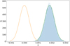 |
Fig. 4 Eccentricity significance. The posterior distribution of the eccentricity is shown in blue. The normal distribution with µ = 0.00188 and σ = 0.00035 in blue is compared to a normal distribution with the same variance but shifted to have its mean at zero (orange curve). The spikes in the posterior distributions are highly investigated regions, such as local minima, where the chains were probably stuck before converging to the global minimum. |
3.2 One-planet models
We modelled together the RV, transit, and occultation midtime data as in Csizmadia et al. (2019) and Bernabò et al. (2024) with an idl script composed of a genetic algorithm minimisation that is followed by a differential evolution Markov chain Monte Carlo (DE-MCMC; Ter Braak 2006). The initial population of the genetic algorithm was composed of 200 individuals. The number of steps of the DE-MCMC procedure was 105 for each of the ten chains. The burn-in phase discards the first 8×10⁴ steps of such a procedure, and the posterior distributions and Gelman-Rubin test were made with the last 2 × 10⁴ iterations.
We first investigated the simplest models to describe our joint dataset: the one-planet circular and eccentric fits, which we partly described in the previous section. We began by fitting a single planet on a circular orbit to the data, which provided an initial baseline model. This approach assumes that the planet’s orbit is perfectly circular, simplifying the mathematical representation and reducing the number of parameters. The fitting parameters were the RV semi-amplitude K and the offset Vγ as well as the instrumental offsets Vinstr for each RV dataset and the orbital period P, while the first transit epoch T0 was assumed as in Hellier et al. (2011): T0 = 5528.86823 BJDTDB. Without the inclusion of photometric and RV jitters, with 471 data points and 15 fitting parameters, we obtained a BIC value of ≃2190 and an AIC of ≃2132. However, the circular fit may not fully capture the dynamics of the system and tidal interactions that can take place. In the one-planet eccentric fit, two extra fitting parameters were included:  and
and  , as described in the previous section. For this fit, the BIC value is ≃ 1855 and AIC≃1789.
Tidal decay results in literature.
3.3 Tidal decay model
A typical effect that can appear in systems showing a strong tidal interaction between the host star and the planet, such as in WASP-12 (Yee et al. 2020 and references therein), is tidal decay of the planetary orbit. Tidal decay has been investigated in WASP-43b via transit timing variations. Some authors have claimed the detection of tidal decay in the system, while other studies discarded it or provided an upper limit. Table 4 summarises the findings of previous studies. Among these studies, we point out that Chen et al. (2014) found a decay rate of −0.09 ± 0.04 s yr−1; however, the BIC criterion does not prefer the quadratic fit over the linear fit. Ricci et al. (2015) obtained a decay rate of −0.021 ± 0.022 s yr−1, but the small difference in χ2 between the linear and the quadratic fits of the transit timing variations (TTVs) shows that statistically the latter brings no significant improvement.
Figure 5 shows the literature values for the tidal decay rate and our result. We took the cycle number as the last transit event considered by the corresponding paper. We highlight the decreasing decay rate (and relative error bars with time).
We investigated the tidal decay scenario by fitting RVs and TTVs simultaneously for the first time and using the longest dataset available (≃10 years). We implemented the script considering that the anomalistic period Pa is a linearly time-varying parameter with a time derivative Ṗa: Pa(t) = Pa,0 + Ṗa(t − T0), where T0 represents the first transit epoch and is not a fitting parameter but fixed to T0 = 5528.86823 BJDTDB (Hellier et al. 2011). The term Ṗa is linked to the change in the RV semi-amplitude  and through Kepler’s Third Law to the time derivative of the semi-major axis ȧ:
 (3)
(3)
The RV curve now has the addition of the semi-amplitude K(t) as a time-varying parameter, where its time-derivative  is derived from the combination of Equation (3) and the well- known definition of K:
 (4)
(4)
where q is the planet-to-star mass ratio and i is the orbital inclination.
We fitted the TTVs with a quadratic trend, as in Equations (4) and (5) of Harre et al. (2023) or as the third term of Equation (7). We obtained a tidal decay rate of (−1.85 ± 0.51) ms yr−1, which is compatible with the value of Section 3.6. With 17 fitting parameters, the BIC value is ≃ 1946 and the AIC is ≃1876.
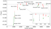 |
Fig. 5 Literature retrievals of tidal decay rate and our results plotted as a function of cycle number starting from Hellier et al. (2011) as epoch zero. Non-detections are shown in red, detections are in green, and cases where there is only an upper limit are in grey. A zoom-in of the region between cycle numbers 2000 and 6000 is provided to show the small error bars of the latest studies. Our result is shown in green because even if BIC and AIC disfavour the tidal decay fit in comparison to the one- planet eccentric fit, in Section 3.6 we detect the same tidal decay rate, and this fit is the preferred one. The error bar on our value is particularly small because we fit TTVs and RVs simultaneously and because we make use of the longest dataset available. |
Contributions to the periastron precession rate.
3.4 Long-term acceleration model
The next step in our analysis involved extending the model to consider the possibility of additional bodies in the system (see also Section 4.2). In this case, the RV model included an extra long-term acceleration  , as in Bernabò et al. (2024) and in Equation (6), which resulted in
  km s−1, compatible with zero within the error bars as well as with the result of Section 3.6 in Table 6. With 17 fitting parameters, the BIC value of this fit is ≃ 1898 and the AIC value is ≃1828.
3.5 Periastron precession model
We first calculated the expected contributions of the apsidal motion rate as  , where the orbital periastron angle varies linearly with time and where the rate of apsidal motion
  is the sum of the general relativity, tidal, and rotational contributions:
 (5)
(5)
(see Equations (1)–(5) and the Appendix in Bernabò et al. (2024) for more details). Such contributions are explicitly written in Appendix A of Bernabò et al. (2024). Here, we calculated them for WASP-43b, and they are reported in Table 5. We note that the planetary contributions were computed assuming synchronous rotation of the planet (Porb/Prot,p = 1) and the two extreme cases for the planetary internal structure: the Love number of the planet k2,p = 0.01 and k2,p = 1.5. Specifically, k2,p = 0.01 represents an extreme case where the planet behaves almost as a point mass with minimal deformation, suggesting a highly rigid body with negligible tidal bulging. On the other hand, k2,p = 1.5 stands for a fluid-like homogeneous body that experiences significant deformation under tidal forces. The main contribution is the planetary one (see Equation (8) and relative discussion in Ragozzine & Wolf 2009), and the total periastron precession rate ranges then from ≃ 3″ to ≃146″, respectively in the case of k2,p = 0.01 and k2,p = 1.5, while the period of such a motion ranges from ≃1037 to ≃24 years.
As in the case of WASP-19Ab, we fitted a precessing orbit in RVs and TTVs using Equations (7) and (8) of Bernabò et al. (2024) for the RV fitting and Equations (7) and (8) of Csizmadia et al. (2019) for transits and occultations. As in Bernabò et al. (2024), we initially applied the semi-grid method, which involves fixing one parameter (the periastron precession rate) at several distinct values while systematically varying other parameters. It is particularly useful for isolating the impact of specific factors in complex models. In the fitting, we kept  fixed at 48 different values between −0.30 and +0.30° d−1 while focusing around
  in particular. Figure 6 shows the fit results with the corresponding chi-squared values. Many local minima appear, revealing the complexity of the problem.
This preliminary analysis allowed us to identify key trends and then proceed to free  for fitting, leading to a comprehensive analysis. We obtained a periastron precession rate of
  d−1 = (602.98±29.79)″ d−1. This values corresponds to the global minimum found in Figure 6. The BIC value of such a fit is ≃1886 and the AIC is ≃1816. We highlight that
  is well above the highest limit of ≃145″ d−1 calculated for k2,p = 1.5. The implications of this result will be discussed in Section 4.
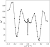 |
Fig. 6 Results of the semi-grid analysis with a fixed periastron precession rate at 48 different values and the χ2 of the corresponding fit (relative to the minimum χ2). |
3.6 Complete model
Finally, we implemented the RV and TTV fitting model of Bernabò et al. (2024) with a joint fit of an RV long-term acceleration in the RV trend and tidal decay and periastron precession. The complete RV equation is
![Mathematical equation: $\matrix{ {V(t) = {V_{i,instr}} + {V_\gamma } + {{\dot V}_\gamma } \cdot \left( {t - {t_0}} \right) + \delta V(t)} \cr { + K(t) \cdot [e \cdot \cos (\omega (t)) + \cos (\v (t) + \omega (t))],} \cr } $](/articles/aa/full_html/2025/02/aa51994-24/aa51994-24-eq62.png) (6)
(6)
where Vi,instr is the instrumental offset (i indicates the ID number of the dataset, as in Table 3), Vγ is the systematic velocity of the barycentre of the exoplanetary system,  is the long-term acceleration, and δV is the apparent contribution due to the distorted stellar shape (see Equation (10) and relative discussion in Bernabò et al. 2024). The term υ(t) is the angle describing the true anomaly of the orbit, while ω(t) and K(t) represent the time-changing functions of the periastron angle and of the RV semi-amplitude, respectively. We note that ω(t) varies linearly with time due to the apsidal motion:
  . The second term, K(t), is not a fitting parameter but is derived from the linear change in the anomalistic period Pa(t), as described in Section 3.3.
We implemented the TTV fitting model of Csizmadia et al. (2019) and Bernabò et al. (2024) by allowing both tidal decay and periastron precession to be fit at the same time. In particular, transit mid-times were then fitted as
 (7)
(7)
where Ntr is the transit (or cycle) number, as in the first column of Table A.1. The term Ps(t) represents the time-changing sidereal period, which is derived from the anomalistic period with their relation Ps(t) =  , where n(t) is the mean motion and
  . The first two terms of the equation represent the linear fit, the third one is the quadratic fit (tidal decay), and the last one is the periastron precession. Occultations were fitted in the same way, substituting Ntr with Nocc, with a positive sign before the last term and with an additional + Ps(t)/2 term to account for the half orbit that the planet has travelled between the transit and the occultation event.
The results of the joint fit (RVs, transit, and occultation midtimes), including apsidal motion, tidal decay, and long-term acceleration, can be found in Table 6, which also reports the median values and 1σ uncertainty for each fitting parameter. For  and Ṗa, we also report the 2σ confidence levels. As discussed in Section 3.1, since the eccentricity is a key parameter for our study and an eccentric orbit is a precondition for periastron precession to take place, we report the 2σ and 5σ error bars for e. Figure 7 shows the phase-folded RV data and residuals of this complete model. Figure 8 shows the mid-transit and midoccultation timing residuals, which present no visible deviation from a zero trend.
We detected a periastron precession rate of  , which is com patible with the result in Section 3.5. As in Bernabò et al. (2024), a small number of the MCMC chains converged to the same value but with a negative sign, showing how complex the convergence of such a fitting is. Within the error bars, the positive
  rate agrees with the result of the periastron precession fit in Section 3.5. The tidal decay rate is Ṗa = (−1.99 ± 0.50) ms yr−1 = (−0.00195 ± 0.00050) s yr−1, which is in agreement with the result of the tidal decay fit of Section 3.3. We attribute such small error bars (≃5% for
  and ≃27% for Ṗa) to the fact that for the first time we simultaneously fitted RVs and TTVs and to the long and wide baseline with respect to all previous papers that investigated tidal decay.
Figure 9 shows such contributions in TTVs over time. The contributions of apsidal motion in transit and occultation midtimes have an opposite phase, as in Equation (7). In certain regions, tidal decay and apsidal motion can cancel each other, making it hard to distinguish the two if a long enough baseline of observations is not available. Even if the amplitude of the contribution of apsidal motion is smaller than the error bars of some of the transit and occultation mid-times, the detection of apsidal motion is possible due to the combination of RV and TTV analysis and the length of the database (≃10 years) and the number of data points (471 transits, occultations, and out-of-transit RVs) we used.
This rate of tidal decay corresponds to an increase of the RV semi-amplitude  . We did not detect a linear trend (long-term acceleration
  ), which supports the fact that there is no unseen third body in the system (see Section 4 for a complete analysis). The apsidal motion has a period of
  years, meaning that the periastron angle ω has completed two cycles within the length of our observations. As shown in Table 7, with 19 fitting parameters, the BIC value is ≃ 1849 and for the AIC it is ≃ 1771. Statistically, this is the favoured model, even if it has the highest number of parameters. With the inclusion of the jitters – which are adjusted post-fitting – the joint fit has a reduced χ2 of ≃ 0.97.
Figure 10 shows the posterior distributions of the most critical fitting parameters (considering only the last 2 × 10⁴ steps of the DE-MCMC procedure, excluding the burn-in phase). In the top plot, we show the relation between the anomalistic period and the periastron precession rate. These two parameters are one of the more correlated and degenerate parameter pair in our model due to the well-known equation  , where Ps(t), Pa(t) and n(t) are time-varying parameters. The middle plot shows the correlation between the tidal decay rate and the rate of the RV semi-amplitude change
  , as in Equation (4). The lower plot shows the posterior distributions of
  and Ṗa, which appear to not to be correlated.
The high periastron precession rate of  has never been observed in any exo planetary system. Even with orbital parameters similar to WASP-18Ab (Csizmadia et al. 2019) and WASP-19Ab (Bernabò et al. 2024), it is ≃20 times bigger with respect to the former and almost three times bigger than the latter. In the next section, we discuss some possible causes of such a high detected rate of apsidal motion.
Results of the complete fit.
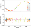 |
Fig. 7 RV curve. Top plot: phase-folded RV data with a periastron precession rate of 0.1727° d−1 and residuals, with a standard deviation of ≃ 13.5 m s−1. |
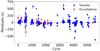 |
Fig. 8 Residuals of transit and occultation mid-times with a standard deviation of ≃ 127.4 and 155.6 s, respectively. |
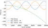 |
Fig. 9 Transit timing variations caused by the measured tidal decay (dashed-dotted line in green) and apsidal motion contributions (respectively in blue for transit mid-times and orange for occultation mid-times) for the ≃ 10 years of transit and occultation data used in this paper. |
Model comparison.
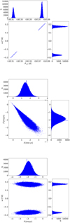 |
Fig. 10 Posterior distribution of the parameters for all ten chains, excluding the DE-MCMC steps in the burn-in phase. Top plot: correlation between the anomalistic period and the periastron precession rate. A small number of chains were stuck in a local minimum with the same value as the detected |


4 Discussion
4.1 WASP-43b is a fast rotator
Once the periastron precession rate was measured, we subtracted the general relativity term and the tidal and rotational components relative to the star from the observed value (see Equation (5)). As described in Appendix A of Bernabò et al. (2024), the remaining terms are the tidal and rotational contributions of the planet, whose first orders approximation are
 (8)
(8)
and
 (9)
(9)
where M★ and mp are the stellar and planetary masses, rp is the planetary radius (see also Sterne 1939), k2,★ and kշ,p are the fluid Love numbers of the star and planet, and Prot,★ and Prot,p are the stellar and planetary rotation period around their own axis. The other parameters have been defined already.
The equations depend on two unknowns: k2,p and Prot,p. To solve the equations for k2,p, we have to assume Prot,p. The two extreme cases are when the planet rotates at the break-up velocity – corresponding to Prot,p ≃ 2.18 hours – and when it is not rotating (Fp = Pa /Prot,p →0).
The observed apsidal motion rate is four times the maximum rate in Table 5, which is calculated assuming synchronisation of the planetary rotational and orbital periods Prot,p = Porb (or Fp = 1). With this assumption, the Love number we derived is much higher than the physical limit of 1.5, which corresponds to a homogeneous body. No physical solution to the previous equations was found with such an assumption. Therefore, we relaxed the assumption and calculated solutions for the parameter couple k2,p and Prot,p, which are plotted in Figure 11. The red, green, and blue areas represent all such solutions, within the 1σ, 2σ, and 3σ error bars for  , respectively. The grey area above kշ,p = 1.5 contains unphysical solutions (representing interior structure models with an envelope denser than the core). The three vertical lines respectively denote the cases of a nonrotating planet, synchronous rotation, and the extreme scenario of break-up velocity.
By solving for the parameter couple (k2,p, Prot,p), we can therefore provide a range for k2,p depending on Prot,p. Figure 11 suggests that WASP-43b is a fast rotator with a lower limit on Prot,p ≳ 4.26 hours (for Fp ≃ 4.58, the lowest 3σ limit visible in the Figure) and on k2,p ≳ 2.18 hours (the lowest 3σ limit in correspondence of Fp ≃ 8.95, when the planet is rotating at the break-up velocity).
The fact that WASP-43b may rotate faster than expected could be caused by the impact of a massive object. A significant collision with a large celestial body could have imparted additional angular momentum to the planet, thereby increasing its rotational speed, as it is believed that Earth’s relatively rapid rotation and the formation of the Moon resulted from a colossal impact with a Mars-sized object in the early stages of its development (see Daly 1946 and references therein). Such impacts are not uncommon in the chaotic environments of young planetary systems, where collisions can significantly influence the rotational dynamics of planets. Alternatively, processes within the planet’s mantle or core, such as vigorous convection or dynamic core movements, can redistribute mass internally, altering the planet’s moment of inertia and potentially leading to changes in its rotation rate over time.
In most cases of such a tight orbit, we can reasonably assume that during the lifetime of the system, the orbit has been synchronised due to gravitational tidal forces. As Rauscher et al. (2023) shows, assuming Jupiter’s quality factor and its initial rotational state, planets with an orbital period below ≃ 30 days have a synchronisation time scale of ≲4 Gyrs and are supposed to be aligned and synchronised. However, the age of WASP-43 is not known. Scandariato et al. (2022) reports an age of  Gyr from isochrones, while Gallet & Delorme (2019)’s tidal-chronology technique derives a range between 2.4 and 9.2 Gyr, and Hellier et al. (2011) calculates the gyrochronological age as
  Myr from the stellar rotation period. Since the planetary orbit is tidally decaying, this estimate may not be entirely reliable, as the host star could be spun up, making the derived age appear younger than the actual age (see, e.g., Maxted et al. 2015). Moreover, the planetary orbit is eccentric, with e = 0.00188±0.00035, even though the planet orbits very close to the host star. This is the only ultra-short period planet whose orbit is eccentric (see Section 3.1) and that does not appear to have a companion star or planet that can drive the eccentricity, as in the case of WASP-19Ab (see Appendix B in Bernabò et al. 2024). Therefore, the orbit may have not been circularised by tidal forces yet. This supports the hypothesis of a young system since the typical circularisation time scale has an order of magnitude of 10−3 Gyr (derived from Equation (5) in Charalambous et al. 2023 assuming Jupiter’s quality factor and Love number k2, in agreement with Terquem & Martin 2021). If the orbit is not circularised yet, it may also not be synchronised yet.
The JWST light curve published and analysed by Bell et al. (2024) does not support this hypothesis. If the planet rotates about four times faster than its orbital velocity, there should not be a big temperature gradient between the day side and the night side of the planet. However, Bell et al. (2024) detected a day-tonight temperature contrast of ≃ 700 K. On the other hand, Lesjak et al. (2023) recovered a line broadening in the atmosphere corresponding to an equatorial velocity of  km s−1, or equivalently a rotational period of
  hours. Assuming tidal locking, such a detected velocity is larger than the synchronous rotational velocity. The paper claims that it is indicative of a super-rotating equatorial jet with a velocity of
  km s−1. Unless the planet rotational axis is tilted with respect to the orbital plane, these recent findings may also be favourable to a faster rotational period than the synchronous one. Moreover, Stevenson et al. (2017) and Scandariato et al. (2022) report offsets of a hotspot measured as (21.1 ± 1.8)° from the Spitzer phase curve and
  from the CHEOPS phase curve, respectively. These results suggest that the rotation rate of the hotspot is not consistent with a tidally locked state (Penn & Vallis 2018). However, it is unclear whether the rotation rate of the hotspot directly represents the rotation rate of the planet. (For a detailed discussion on the relationship between wind rotation rates and the planetary rotation at different pressure levels, see Carone et al. 2020). If the hotspot’s rotation rate indeed corresponds to the planetary rotation rate, this would be an indication that the planet is not tidally locked. More observations are needed in this direction, such as future RM measurements on the planet to detect the inclination of its rotational axis.
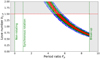 |
Fig. 11 Couples of period ratio and Love number of the planet that solve Equations (8) and (9). The blue and light blue points correspond to a combination of (Fp, k2,p) that satisfies the observed periastron precession rate within its 1σ, 2σ, and 3σ error bars (red, green, and blue areas, respectively). The red horizontal line represents the physical limit where the body is homogeneous. From left to right, the three vertical lines highlight a non-rotation planet (Porb/Prot,p →0), synchronous rotation (Prot,p = Porb), and the break-up limit (Prot,p ≃ 8.95 Porb, corresponding to Prot,p ≃ 2.18 hours). The grey shaded regions are unphysical. |
4.2 Presence of a third unseen body
In this section, we discuss if the observed periastron precession rate can be explained by the presence of a third not yet discovered body in the system (e.g. a companion star or planet).
We searched Gaia DR3 (Gaia Collaboration 2016; Vallenari et al. 2022) for possible co-moving companions to WASP-43 using the same method that revealed probable bound companions to WASP-18A (Csizmadia et al. 2019) and WASP-19A (Bernabò et al. 2024). Searching to a projected separation of ≃ 105 AU (19.2″), we found no candidates with parallax and proper motion values consistent (even to 10σ) with those of WASP-43. As far as the Gaia DR3 evidence goes, WASP-43 is an isolated single star.
As also done in Bernabò et al. (2024), we fitted the RV datasets separately with an additional Keplerian signal beyond that of planet b in order to mimic a hypothetical candidate companion in the system. We ‘injected’ the candidate into the RV fitting model with different random orbital parameters (orbital period, RV semi-amplitude,  , and
, and  ). We randomly varied the other orbital parameters as follows:
  and
and  between -1.0 and 1.0, the RV semi-amplitude Kc between 0.1 (the minimum RV error bar) and 125 m s−1 (the maximum RV residual after the subtraction of planet b).
We applied this analysis to the datasets with a large number of data and well-spread observations in time. We selected datasets with a length of at least a few days: IDs 1, 2, 4, and 8. We also applied it to the whole RV dataset after removing the offsets from each dataset. We investigated 2 × 10⁸ random candidates for each separate dataset and 109 for the complete data collection. The orbital period of the candidate was constrained to avoid collisions with the star (see Equation (6) of Bernabò et al. 2024) and to be shorter than the duration of the observations of the corresponding datasets (approximately 187 days for ID 1, 38 days for ID 2, 782 days for ID 4, 18 days for ID 8, and 10 years for the complete RV set). The results of the analysis are shown in Figure 12, where we plot the orbital period of such a candidate against the χ2 of the corresponding fit, coloured by planetary mass. All candidates have a mass below 45ME, and 90% of them have mc smaller than 20ME , showing that only a very small mass companion could be ‘hidden’ in the RV signal. Moreover, via the BIC, we calculated the χ2 value that needs to be reached to have (at least) weak evidence that a two-planet fit is better than a single-planet fit. The red dashed line in the figure denotes such a value. Our analysis did not retrieve the presence of any candidate body that passes the BIC threshold, according to Kass & Raftery (1995) criterions.
In order to exclude any putative planetary companion in the system, we also used the l1 periodogram analysis (Hara et al. 2017), which is similar to the Lomb–Scargle periodogram and was specifically designed to search for periodicities in radial velocities. We applied it to the whole RV dataset, separately on the single datasets and on the residuals after subtracting the RV signal produced by planet b, as shown in the top and bottom plots of Figure 13, respectively. In both cases, the in-transit points are excluded from the analysis. In the first case, the only significant peak with a false alarm probability (FAP) smaller than 1% is the one at 0.81 days, which is the orbital period of WASP-43b. The periodogram of the residuals does not show any significant peak passing the FAP test, with a threshold at 1%, meaning that only 1% of the periodograms calculated on random noise would have a peak amplitude equal to or greater than that observed in the periodogram. The peaks most probably relate to an artefact in the data instead of a true period (see also the different y-amplitudes between the two plots).
We also report a sensitivity analysis based on the Rømer effect (or light time effect; Irwin 1952). If TTVs are due to an outer companion, this would cause the system’s centre of mass to be shifted. The observed mid-transit and occultation times are affected by the time difference that it takes the light to travel from the far side to the near side of the orbit with respect to the observer (see the case of WASP-4b in Harre & Smith 2023, where the apparent tidal decay is explained by the light travel effect). For circular orbits, the TTV amplitude ∆t due to such an effect is (Schneider 2005):
 (10)
(10)
Subtracting the TTV signal of planet b, the maximum TTV residual is ≃600 s, which is set as ∆t in the equation. With this assumption, we calculated the corresponding putative planetary mass by changing its orbital period of WASP-43b from the period of WASP-43b (since it is an outer companion) to the length of the transit dataset (≃3 700 days). We also considered the possibility that only a part of the TTV residuals is due to the Rømer effect and accounted for scenarios where ∆t = 10, 25, 50, and 75% of such a TTV amplitude. Additionally, we considered the hypothesis that the periastron precession rate we observe in Section 3.6 could be caused by the presence of a planet. The amplitude of the TTVs caused by an apsidal motion of 0.1727° d−1 results in ≃39 s. Therefore, we also assumed ∆t = 39 s and repeated the study (see the blue line in Figure 14). Figure 14 illustrates the relationship between the orbital period and the planetary mass. It also shows the mass of a planet that could shift the system’s center of mass and generate such a TTV amplitude. The two horizontal lines in the figure mark the minimum brown dwarf and stellar masses. The upper shaded grey area in the plot indicates the region where a hypothetical planet with a given period and mass would be detectable by our RV data. Specifically, this area indicates the parameter space where any such planet would produce a radial velocity signal that exceeds the residuals left after subtracting the known planet b(≃125 m s−1). Consequently, if a planet with these parameters existed, it would likely have been detected.
In determining the detection threshold of our study, we considered the typical error of the RV data (conservatively, we took their median ≃5 m s−1). The lower grey shaded region in Figure 14 delineates the parameter space where hypothetical planets would induce a radial velocity semi-amplitude smaller than the indicated threshold. A hypothetical planet could potentially reside in the lower shaded region and still be undetected, having a mass mc less than ≃0.3 MJ. The exact limiting value of mass depends on its combination with the orbital period value, as seen in the figure.
We also estimated the mass and period of a hypothetical third body contributing to the detected apsidal motion rate using Equation (12) from Borkovits et al. (2011) in case of a co-planar, eccentric outer (Pc>Pb) orbit. Its amplitude is
 (11)
(11)
where mb and mc denote the masses of planet b and the putative companion c, Pb and Pc are their orbital periods, and ec is the orbital eccentricity of body c. We subtracted the general relativity contribution from the detected apsidal motion rate and calculated the mass and orbital period of a planet that would account for the measured  . The results of this analysis are shown in Figure 15, where we vary the eccentricity of the orbit of the putative companion from 0 to 0.8. The two grey shaded areas represent the same sensitivity limits as in Figure 14. Since the upper shaded region encompasses all the plotted periodmass curves, we can exclude the possibility that the observed apsidal motion rate is caused by an unseen second body within the sensitivity limits expressed in the previous paragraph and Figure 14.
In this section, we excluded the possibility of the presence of a companion in the system that may cause the detected high apsidal motion and orbital decay rate. The sensitivity of our analysis depends on the planetary orbital period. It goes down to a fraction of Jupiter’s mass at a period of up to ≃3700 days, which is the length of the time window of our dataset. Moreover, in Sections 3.4 and 3.6, we retrieved a long-term trend in RVs (or long-term acceleration,  ) that is compatible with a non-accelerating system (see Table 6), confirming that there is no hint of a second stellar or planetary body in our dataset.
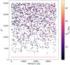 |
Fig. 12 Random candidate planet c fit χ2 against its orbital period. The dashed horizontal lines correspond to the χ2 needed for weak evidence of the presence of a second body, according to the BIC criterion (see text for more details). The candidates are coloured by planetary mass. |
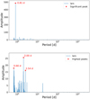 |
Fig. 13 Periodograms of RVs. Top plot: periodogram of the RV dataset showing the only significant peak at ≃0.814 days, corresponding to the orbital period of WASP-43b. Bottom plot: periodogram of the residuals showing the three highest peaks, which do not pass the FAP test with a threshold at 1%. |
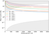 |
Fig. 14 Results of the sensitivity analysis based on the light travel effect. The plot shows the relationship between the orbital period and the planetary mass of a planet responsible for 10, 25, 50, 75, and 100% of the TTVs. The lowest blue curve reflects the possibility that the periastron precession rate observed is caused solely by the Rømer effect (see text for more details). The yellow and brown horizontal lines represent the minimum stellar mass (≃75 MJ) and the minimum brown dwarf mass (≃13 MJ), respectively. The grey shaded regions represent the excluded area by RV analysis. The upper region indicates a hypothetical planet causing an RV amplitude greater than 125 m s−1. The lower region delineates the sensitivity threshold of 5 m s−1 (see text for more details). |
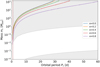 |
Fig. 15 Sensitivity study on the mass and orbital period of a body causing the observed apsidal motion rate of ≃0.1727º d−1 by varying its orbital eccentricity and mass, according to Borkovits et al. (2011). The two grey shaded regions represent the same areas in Figure 14 (see text for more details). The vertical dashed line represents the orbital period of WASP-43b. |
4.3 Stellar inclination
To derive the equations describing the periastron precession (see Appendix A in Bernabò et al. 2024), we assumed that the stellar axis is not (or is only slightly) inclined with respect to the normal of the orbital plane. If this is not the case, additional terms at higher orders can contribute to  (see Kopal 1959, 1978). The contribution of the stellar obliquity term would be an added or subtracted ≃ 10% of the total observed value.
To test such a scenario, we modelled the (Holt-)RM effect (Holt 1893; Rossiter 1924; McLaughlin 1924) in the system to derive the spin-orbit angle of WASP-43. We fitted the whole RV dataset in Table 3 – both in-transit and out-of-transit data – with a C++ script that carries out the analytic calculation for the RM effect by Hirano et al. (2011) as well as the standard RV curve from the planet’s Keplerian orbit. The fitted parameters are the RV semi-amplitude K,  , the stellar rotational velocity υ sin i, the mid-transit time, the sidereal orbital period, the impact parameter, the radius ratio rp/R★, the scaled orbital distance a/R★, the projected stellar obliquity angle λ, and the RV offsets. The best-fitting model and the residuals are shown in Figure 16. In Table 8, we report the results on the fitting parameters. We measured the projected stellar obliquity to be λ = 2.03+1.32°, confirming the results of Esposito et al. (2017) of a well-aligned star.
Results of the RM fit.
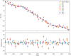 |
Fig. 16 Best-fitting model of the RM effect. Only data points within phase –0.04 and +0.04 are plotted in order to zoom into the transit region. |
5 Conclusions
In this paper, we applied the revised tidal theory of Csizmadia et al. (2019) and Bernabò et al. (2024) on a third case study: the exoplanetary system WASP-43. We acquired new RV data with HARPS and merged this new dataset with the literature and three previously unpublished RV datasets. Together with the RVs, we fitted mid-transit and mid-occultation times from the literature, including the newly acquired JWST phase-curve and the unpublished transits in TESS Sector 62.
We first investigated a simple circular one-planet model and an eccentric one-planet model, finding statistical evidence of a non-zero eccentricity in the orbit. We also investigated three separated scenarios of tidal decay, periastron precession, and long-term acceleration. Since other effects can mimic the consequences of tidal interaction, we ruled out the presence of a perturbing body, such as an extra planet, up to a period of ≃3700 days and down to ≃0.3 MJ and of long-term acceleration in WASP-43.
Finally, we included all the aforementioned effects in our model – long-term acceleration, periastron precession, and tidal decay as a result of the tidal interaction between the planet and the host star. For the first time in an exoplanetary system, we simultaneously detected two outcomes of tidal interactions: tidal decay and apsidal motion. We confirm that the orbit of the system is decaying at a rate of Ṗa = (−1.99 ± 0.50) ms yr−1, and for the first time in the system, we detected apsidal motion at a rate of  .
.
We analysed a broad range of scenarios to explain such a high apsidal motion rate. Assuming a planetary rotational period synchronous to the orbital period – as predicted by the time scale of synchronisation due to tidal interactions – the value of the second-order fluid Love number we derived is above the physical limit of 1.5. We tried to explain the measured  by relaxing the assumption of synchronisation of the planetary rotational period to the orbital period, but this is not supported by the recent JWST findings on the high day-to-night side temperature difference. This scenario could be further investigated in the future with, for example, measurements on the RM effect on the planet and line broadening detections. We also tested the possibility of a contribution to
  from the stellar-inclined spin-orbit axis, but the RM analysis confirmed that the projected obliquity plane is well aligned. We also discarded the presence of a perturber in the system from Gaia DR3 observations, a sensitivity analysis, the study of the l1 periodogram, and from fitting the RV dataset with an extra putative planet. Gaia Data Release 4 may confirm or change the picture by revealing a companion via astrometry.
In conclusion, we have considered various astrophysical scenarios, but most of them encounter difficulties in explaining the results we have obtained. We leave the question open for further investigation while highlighting that in research, the questions raised are often more significant than the answers found, as they drive further inquiry and deeper understanding.
Data availability
Tables A.1, A.2 and B.1 are available in electronic form at the CDS via anonymous ftp to cdsarc.cds.unistra.fr (130.79.128.5) or via https://cdsarc.cds.unistra.fr/viz-bin/cat/J/A+A/694/A233.
Acknowledgements
We acknowledge the support of DFG Research Unit 2440: “Matter Under Planetary Interior Conditions: High Pressure, Planetary, and Plasma Physics” and of DFG grants RA 714/14-1 within the DFG Schwerpunkt SPP 1992, Exploring the Diversity of Extrasolar Planets. A.M.S.S. and J.-V.H. acknowledge support from the Deutsche Forschungsgemeinschaft grant SM 486/2-1 within the Schwerpunktprogramm SPP 1992 “Exploring the Diversity of Extrasolar Planets”. Project no. C1746651 has been implemented with the support provided by the Ministry of Culture and Innovation of Hungary from the National Research, Development and Innovation Fund, financed under the NVKDP-2021 funding scheme. The work is based on observations made with the HARPS instrument on the ESO 3.6-m telescope at La Silla Observatory under programme IDs 089.C−0151, 096.C−0331, 0102.C−0820, 0104.C−0849. This research used the facilities of the Italian Center for Astronomical Archive (IA2) operated by INAF at the Astronomical Observatory of Trieste. This research has made use of the NASA Exoplanet Archive, which is operated by the California Institute of Technology, under contract with the National Aeronautics and Space Administration under the Exoplanet Exploration Program. L.M.B. would like to thank M. Murphy for reanalysing for us Spitzer Space Telescope lightcurves without priors and those observers who provided unpublished transits of WASP- 43b: M. Mifsud, I. Peretto and S. Lora, J.-P. Vignes, S. Foschino, A. Popowicz, M. Szkudlarek, and especially C. Knight, who kindly conducted the observations at his observatory. L.M.B. also acknowledges A. Triaud for the use of the public data used in this work (RV data ID 3) and Nicolas Iro for the interesting discussion on the rotation of WASP-43b.
Appendix A Transit and occultation mid-timings
Tables of transit and occultation mid-times in the literature and used in this work, along with details on the observations.
Mid-transit times.
Mid-occultation times.
Appendix B RV datasets
Table of archive and unpublished RV datasets used in this work.
Radial Velocity datasets used in this work.
References
- Adams, E. R., Jackson, B., Sickafoose, A. A., et al. 2024, PSJ, 5, 163 [NASA ADS] [Google Scholar]
- Akaike, H. 1998, Information Theory and an Extension of the Maximum Likelihood Principle, eds. E. Parzen, K. Tanabe, & G. Kitagawa (New York, NY: Springer), 199 [Google Scholar]
- Baumeister, P., Padovan, S., Tosi, N., et al. 2020, ApJ, 889, 42 [Google Scholar]
- Becker, J. C., & Batygin, K. 2013, ApJ, 778, 100 [NASA ADS] [CrossRef] [Google Scholar]
- Bell, T. J., Crouzet, N., Cubillos, P. E., et al. 2024, Nat. Astron., 8, 879 [Google Scholar]
- Blažek, M., Kabáth, P., Piette, A. A. A., et al. 2022, MNRAS, 513, 3444 [CrossRef] [Google Scholar]
- Bernabò, L. M., Csizmadia, S., Smith, A. M. S., et al. 2024, A&A, 684, A78 [NASA ADS] [CrossRef] [EDP Sciences] [Google Scholar]
- Blecic, J., Harrington, J., Madhusudhan, N., et al. 2014, ApJ, 781, 116 [NASA ADS] [CrossRef] [Google Scholar]
- Bonomo, A. S., Desidera, S., Benatti, S., et al. 2017, A&A, 602, A107 [NASA ADS] [CrossRef] [EDP Sciences] [Google Scholar]
- Borkovits, T., Csizmadia, S., Forgács-Dajka, E., & Hegedüs, T. 2011, A&A, 528, A53 [NASA ADS] [CrossRef] [EDP Sciences] [Google Scholar]
- Carone, L., Baeyens, R., Mollière, P., et al. 2020, MNRAS, 496, 3582 [NASA ADS] [CrossRef] [Google Scholar]
- Carter, J. A., & Winn, J. N. 2009, ApJ, 704, 51 [Google Scholar]
- Charalambous, C., Teyssandier, J., & Libert, A. S. 2023, A&A, 677, A160 [NASA ADS] [CrossRef] [EDP Sciences] [Google Scholar]
- Chen, G., van Boekel, R., Wang, H., et al. 2014, A&A, 563, A40 [NASA ADS] [CrossRef] [EDP Sciences] [Google Scholar]
- Cosentino, R., Lovis, C., Pepe, F., et al. 2012, SPIE Conf. Ser., 8446, 84461V [Google Scholar]
- Csizmadia, S. 2020, MNRAS, 496, 4442 [Google Scholar]
- Csizmadia, S., Hellard, H., & Smith, A. M. S. 2019, A&A, 623, A45 [NASA ADS] [CrossRef] [EDP Sciences] [Google Scholar]
- Csizmadia, S., Smith, A. M. S., Kálmán, S., et al. 2023, A&A, 675, A106 [NASA ADS] [CrossRef] [EDP Sciences] [Google Scholar]
- Daly, R. A. 1946, Proc. Am. Philos. Soc., 90, 104 [Google Scholar]
- Davoudi, F., Bastürk, Ö., Yalçinkaya, S., Esmer, E. M., & Safari, H. 2021, AJ, 162, 210 [NASA ADS] [CrossRef] [Google Scholar]
- Dawson, R. I., & Johnson, J. A. 2018, ARA&A, 56, 175 [Google Scholar]
- Eastman, J., Siverd, R., & Gaudi, B. S. 2010, PASP, 122, 935 [Google Scholar]
- Esposito, M., Covino, E., Desidera, S., et al. 2017, A&A, 601, A53 [NASA ADS] [CrossRef] [EDP Sciences] [Google Scholar]
- Fox, C., & Wiegert, P. 2022, MNRAS, 516, 4684 [NASA ADS] [CrossRef] [Google Scholar]
- Gaia Collaboration (Prusti, T., et al.) 2016, A&A, 595, A1 [NASA ADS] [CrossRef] [EDP Sciences] [Google Scholar]
- Gallet, F., & Delorme, P. 2019, A&A, 626, A120 [EDP Sciences] [Google Scholar]
- Garai, Z., Pribulla, T., Parviainen, H., et al. 2021, MNRAS, 508, 5514 [CrossRef] [Google Scholar]
- Gardner, J. P., Mather, J. C., Clampin, M., et al. 2006, Space Sci. Rev., 123, 485 [Google Scholar]
- Gillon, M., Triaud, A. H. M. J., Fortney, J. J., et al. 2012, A&A, 542, A4 [NASA ADS] [CrossRef] [EDP Sciences] [Google Scholar]
- Goffo, E., Gandolfi, D., Egger, J. A., et al. 2023, ApJ, 955, L3 [NASA ADS] [CrossRef] [Google Scholar]
- Hara, N. C., Boué, G., Laskar, J., & Correia, A. C. M. 2017, MNRAS, 464, 1220 [Google Scholar]
- Harre, J.-V., & Smith, A. M. S. 2023, Universe, 9, 506 [Google Scholar]
- Harre, J. V., Smith, A. M. S., Barros, S. C. C., et al. 2023, A&A, 669, A124 [NASA ADS] [CrossRef] [EDP Sciences] [Google Scholar]
- Hatzes, A. P., & Rauer, H. 2015, ApJ, 810, L25 [Google Scholar]
- Hellier, C., Anderson, D. R., Collier Cameron, A., et al. 2011, A&A, 535, L7 [NASA ADS] [CrossRef] [EDP Sciences] [Google Scholar]
- Hirano, T., Suto, Y., Winn, J. N., et al. 2011, ApJ, 742, 69 [NASA ADS] [CrossRef] [Google Scholar]
- Holman, M. J., & Murray, N. W. 2005, Science, 307, 1288 [Google Scholar]
- Holt, J. R. 1893, Astron. & Astrophys., 12, 646 [NASA ADS] [Google Scholar]
- Hoyer, S., Pallé, E., Dragomir, D., & Murgas, F. 2016, AJ, 151, 137 [NASA ADS] [CrossRef] [Google Scholar]
- Irwin, J. B. 1952, ApJ, 116, 211 [Google Scholar]
- Jiang, I.-G., Lai, C.-Y., Savushkin, A., et al. 2016, AJ, 151, 17 [NASA ADS] [CrossRef] [Google Scholar]
- Kálmán, S., Szabó, G. M., & Csizmadia, S. 2023, A&A, 675, A107 [NASA ADS] [CrossRef] [EDP Sciences] [Google Scholar]
- Kálmán, S., Derekas, A., Csizmadia, S., et al. 2024, A&A, 687, A144 [NASA ADS] [CrossRef] [EDP Sciences] [Google Scholar]
- Kass, R. E., & Raftery, A. E. 1995, J. Am. Statist. Assoc., 90, 773 [CrossRef] [Google Scholar]
- Kataria, T., Showman, A. P., Fortney, J. J., et al. 2015, ApJ, 801, 86 [NASA ADS] [CrossRef] [Google Scholar]
- Kokori, A., Tsiaras, A., Edwards, B., et al. 2022, Exp. Astron., 53, 547 [NASA ADS] [CrossRef] [Google Scholar]
- Kopal, Z. 1959, in The International Astrophysics Series (London: Chapman & Hall) [Google Scholar]
- Kopal, Z. 1978, Dynamics of Close Binary Systems, Astrophysics and Space Science Library (Dordrecht: Reidel) [CrossRef] [Google Scholar]
- Lesjak, F., Nortmann, L., Yan, F., et al. 2023, A&A, 678, A23 [NASA ADS] [CrossRef] [EDP Sciences] [Google Scholar]
- Love, A. E. H. 1911, Some Problems of Geodynamics [Google Scholar]
- Maciejewski, G., Puchalski, D., Saral, G., et al. 2013, Inform. Bull. Variable Stars, 6082, 1 [NASA ADS] [Google Scholar]
- Maciejewski, G., Dimitrov, D., Fernández, M., et al. 2016, A&A, 588, L6 [NASA ADS] [CrossRef] [EDP Sciences] [Google Scholar]
- Maciejewski, G., Golonka, J., Fernández, M., et al. 2024, A&A, 692, A35 [NASA ADS] [CrossRef] [EDP Sciences] [Google Scholar]
- Maxted, P. F. L., Serenelli, A. M., & Southworth, J. 2015, A&A, 577, A90 [NASA ADS] [CrossRef] [EDP Sciences] [Google Scholar]
- Mayor, M., Pepe, F., Queloz, D., et al. 2003, The Messenger, 114, 20 [NASA ADS] [Google Scholar]
- McLaughlin, D. B. 1924, ApJ, 60, 22 [Google Scholar]
- Munk, W. H., & MacDonald, G. J. F. 1960, The Rotation of the Earth; A Geophysical Discussion (Cambridge University Press) [Google Scholar]
- Murgas, F., Pallé, E., Zapatero Osorio, M. R., et al. 2014, A&A, 563, A41 [NASA ADS] [CrossRef] [EDP Sciences] [Google Scholar]
- Murphy, M. M., Beatty, T. G., Roman, M. T., et al. 2023, AJ, 165, 107 [NASA ADS] [CrossRef] [Google Scholar]
- Olenick, R. P., Sweeney, A., Lenzen, P., et al. 2019, Robotic Telescopes, Student Research and Education (RTSRE) Proceedings, 2 [Google Scholar]
- Padovan, S., Spohn, T., Baumeister, P., et al. 2018, A&A, 620, A178 [NASA ADS] [CrossRef] [EDP Sciences] [Google Scholar]
- Patra, K. C., Winn, J. N., Holman, M. J., et al. 2020, VizieR Online Data Catalog: J/AJ/159/150 [Google Scholar]
- Penn, J., & Vallis, G. K. 2018, ApJ, 868, 147 [NASA ADS] [CrossRef] [Google Scholar]
- Poddaný, S., Brát, L., & Pejcha, O. 2010, New A, 15, 297 [CrossRef] [Google Scholar]
- Ragozzine, D., & Wolf, A. S. 2009, ApJ, 698, 1778 [Google Scholar]
- Rauscher, E., Cowan, N. B., & Luger, R. 2023, AJ, 165, 261 [NASA ADS] [CrossRef] [Google Scholar]
- Ricci, D., Ramón-Fox, F. G., Ayala-Loera, C., et al. 2015, PASP, 127, 143 [NASA ADS] [CrossRef] [Google Scholar]
- Ricker, G. R., Vanderspek, R., Winn, J., et al. 2016, SPIE Conf. Ser., 9904, 99042B [NASA ADS] [Google Scholar]
- Rossiter, R. A. 1924, ApJ, 60, 15 [Google Scholar]
- Saha, S., Chakrabarty, A., & Sengupta, S. 2021, AJ, 162, 18 [CrossRef] [Google Scholar]
- Scandariato, G., Singh, V., Kitzmann, D., et al. 2022, A&A, 668, A17 [NASA ADS] [CrossRef] [EDP Sciences] [Google Scholar]
- Schneider, J. 2005, in The Light-Time Effect in Astrophysics: Causes and cures of the O–C diagram, ed. C. Sterken, Astronomical Society of the Pacific Conference Series, 335, 191 [NASA ADS] [Google Scholar]
- Schwarz, G. 1978, Ann. Statist., 6, 461 [Google Scholar]
- Seager, S., Kuchner, M., Hier-Majumder, C. A., & Militzer, B. 2007, ApJ, 669, 1279 [NASA ADS] [CrossRef] [Google Scholar]
- Serrano, L. M., Gandolfi, D., Mustill, A. J., et al. 2022, Nat. Astron., 6, 736 [NASA ADS] [CrossRef] [Google Scholar]
- Silverstein, M. L., Barclay, T., Schlieder, J. E., et al. 2024, AJ, 167, 255 [NASA ADS] [CrossRef] [Google Scholar]
- Sotin, C., Grasset, O., & Mocquet, A. 2007, Icarus, 191, 337 [Google Scholar]
- Sterne, T. E. 1939, MNRAS, 99, 451 [NASA ADS] [Google Scholar]
- Stevenson, K. B., Désert, J.-M., Line, M. R., et al. 2014, Science, 346, 838 [Google Scholar]
- Stevenson, K. B., Line, M. R., Bean, J. L., et al. 2017, AJ, 153, 68 [NASA ADS] [CrossRef] [Google Scholar]
- Sun, Z., Ji, J.-h., & Dong, Y. 2018, Chinese Astron. Astrophys., 42, 101 [CrossRef] [Google Scholar]
- Ter Braak, C. J. F. 2006, Statist. Comput., 16, 239 [Google Scholar]
- Terquem, C., & Martin, S. 2021, MNRAS, 507, 4165 [CrossRef] [Google Scholar]
- Valencia, D., O’Connell, R. J., & Sasselov, D. 2006, Icarus, 181, 545 [Google Scholar]
- Vallenari, A., Arenou, F., Bellazzini, M., et al. 2022, Gaia DR3 Documentation, Chapter 19: Performance verification, Gaia DR3 documentation, European Space Agency; Gaia Data Processing and Analysis Consortium. Online at https://gea.esac.esa.int/archive/documentation/GDR3/index.html, id. 19 [Google Scholar]
- Wang, W., van Boekel, R., Madhusudhan, N., et al. 2013, ApJ, 770, 70 [NASA ADS] [CrossRef] [Google Scholar]
- Wang, X.-Y., Wang, Y.-H., Wang, S., et al. 2021, ApJS, 255, 15 [NASA ADS] [CrossRef] [Google Scholar]
- Weaver, I. C., López-Morales, M., Espinoza, N., et al. 2020, AJ, 159, 13 [Google Scholar]
- Winn, J. N. 2010, in Exoplanets, ed. S. Seager, 55 [Google Scholar]
- Wong, I., Shporer, A., Daylan, T., et al. 2020, AJ, 160, 155 [Google Scholar]
- Yee, S. W., Winn, J. N., Knutson, H. A., et al. 2020, ApJ, 888, L5 [Google Scholar]
- Zahn, J. P. 2008, in EAS Publications Series, 29, eds. M. J. Goupil, & J. P. Zahn, 67 [NASA ADS] [CrossRef] [EDP Sciences] [Google Scholar]
All Tables
All Figures
|
Fig. 1 James Webb Space Telescope transit and occultations. Top plot: JWST full-phase observations in time. Middle plot: phase-folded data points in black and best fit in red. To keep the figure clean, error bars are not plotted, but a typical error bar value is shown at the location (0.2,0.98). Grey points are the same as black points but shifted by ±1.0 in phase to make the full phase clearer. Bottom plot: residuals of the fit, after having subtracted the red noise, with a standard deviation of ≃0.00097. |
| In the text | |
|
Fig. 2 Sector 62 of TESS. Top plot: TESS 120-second full-phase observations in time. Middle plot: phase-folded data points in black and best fit in red. The typical error bar value is shown at the location (0.2,0.98). Grey points are shifted by ±1.0 in phase. The occultation is slightly visible at phase ≃0.5. Bottom plot: residuals of the fit, after having subtracted the red noise, with a standard deviation of ≃0.0017. |
| In the text | |
|
Fig. 3 Previously published and new radial velocity observations of WASP-43. The different datasets are plotted with different colours showing the time distribution of the RV observations. |
| In the text | |
|
Fig. 4 Eccentricity significance. The posterior distribution of the eccentricity is shown in blue. The normal distribution with µ = 0.00188 and σ = 0.00035 in blue is compared to a normal distribution with the same variance but shifted to have its mean at zero (orange curve). The spikes in the posterior distributions are highly investigated regions, such as local minima, where the chains were probably stuck before converging to the global minimum. |
| In the text | |
|
Fig. 5 Literature retrievals of tidal decay rate and our results plotted as a function of cycle number starting from Hellier et al. (2011) as epoch zero. Non-detections are shown in red, detections are in green, and cases where there is only an upper limit are in grey. A zoom-in of the region between cycle numbers 2000 and 6000 is provided to show the small error bars of the latest studies. Our result is shown in green because even if BIC and AIC disfavour the tidal decay fit in comparison to the one- planet eccentric fit, in Section 3.6 we detect the same tidal decay rate, and this fit is the preferred one. The error bar on our value is particularly small because we fit TTVs and RVs simultaneously and because we make use of the longest dataset available. |
| In the text | |
|
Fig. 6 Results of the semi-grid analysis with a fixed periastron precession rate at 48 different values and the χ2 of the corresponding fit (relative to the minimum χ2). |
| In the text | |
|
Fig. 7 RV curve. Top plot: phase-folded RV data with a periastron precession rate of 0.1727° d−1 and residuals, with a standard deviation of ≃ 13.5 m s−1. |
| In the text | |
|
Fig. 8 Residuals of transit and occultation mid-times with a standard deviation of ≃ 127.4 and 155.6 s, respectively. |
| In the text | |
|
Fig. 9 Transit timing variations caused by the measured tidal decay (dashed-dotted line in green) and apsidal motion contributions (respectively in blue for transit mid-times and orange for occultation mid-times) for the ≃ 10 years of transit and occultation data used in this paper. |
| In the text | |
|
Fig. 10 Posterior distribution of the parameters for all ten chains, excluding the DE-MCMC steps in the burn-in phase. Top plot: correlation between the anomalistic period and the periastron precession rate. A small number of chains were stuck in a local minimum with the same value as the detected |
| In the text | |
|
Fig. 11 Couples of period ratio and Love number of the planet that solve Equations (8) and (9). The blue and light blue points correspond to a combination of (Fp, k2,p) that satisfies the observed periastron precession rate within its 1σ, 2σ, and 3σ error bars (red, green, and blue areas, respectively). The red horizontal line represents the physical limit where the body is homogeneous. From left to right, the three vertical lines highlight a non-rotation planet (Porb/Prot,p →0), synchronous rotation (Prot,p = Porb), and the break-up limit (Prot,p ≃ 8.95 Porb, corresponding to Prot,p ≃ 2.18 hours). The grey shaded regions are unphysical. |
| In the text | |
|
Fig. 12 Random candidate planet c fit χ2 against its orbital period. The dashed horizontal lines correspond to the χ2 needed for weak evidence of the presence of a second body, according to the BIC criterion (see text for more details). The candidates are coloured by planetary mass. |
| In the text | |
|
Fig. 13 Periodograms of RVs. Top plot: periodogram of the RV dataset showing the only significant peak at ≃0.814 days, corresponding to the orbital period of WASP-43b. Bottom plot: periodogram of the residuals showing the three highest peaks, which do not pass the FAP test with a threshold at 1%. |
| In the text | |
|
Fig. 14 Results of the sensitivity analysis based on the light travel effect. The plot shows the relationship between the orbital period and the planetary mass of a planet responsible for 10, 25, 50, 75, and 100% of the TTVs. The lowest blue curve reflects the possibility that the periastron precession rate observed is caused solely by the Rømer effect (see text for more details). The yellow and brown horizontal lines represent the minimum stellar mass (≃75 MJ) and the minimum brown dwarf mass (≃13 MJ), respectively. The grey shaded regions represent the excluded area by RV analysis. The upper region indicates a hypothetical planet causing an RV amplitude greater than 125 m s−1. The lower region delineates the sensitivity threshold of 5 m s−1 (see text for more details). |
| In the text | |
|
Fig. 15 Sensitivity study on the mass and orbital period of a body causing the observed apsidal motion rate of ≃0.1727º d−1 by varying its orbital eccentricity and mass, according to Borkovits et al. (2011). The two grey shaded regions represent the same areas in Figure 14 (see text for more details). The vertical dashed line represents the orbital period of WASP-43b. |
| In the text | |
|
Fig. 16 Best-fitting model of the RM effect. Only data points within phase –0.04 and +0.04 are plotted in order to zoom into the transit region. |
| In the text | |
Current usage metrics show cumulative count of Article Views (full-text article views including HTML views, PDF and ePub downloads, according to the available data) and Abstracts Views on Vision4Press platform.
Data correspond to usage on the plateform after 2015. The current usage metrics is available 48-96 hours after online publication and is updated daily on week days.
Initial download of the metrics may take a while.