| Issue |
A&A
Volume 694, February 2025
|
|
|---|---|---|
| Article Number | A116 | |
| Number of page(s) | 15 | |
| Section | Planets, planetary systems, and small bodies | |
| DOI | https://doi.org/10.1051/0004-6361/202451767 | |
| Published online | 07 February 2025 | |
Euclid: Detecting Solar System objects in Euclid images and classifying them using Kohonen self-organising maps★
1
Department of Mathematics and Physics E. De Giorgi, University of Salento,
Via per Arnesano, CP-I93,
73100
Lecce,
Italy
2
INFN, Sezione di Lecce,
Via per Arnesano, CP-193,
73100
Lecce,
Italy
3
INAF-Sezione di Lecce, c/o Dipartimento Matematica e Fisica,
Via per Arnesano,
73100
Lecce,
Italy
4
European Space Agency/ESRIN,
Largo Galileo Galilei 1,
00044
Frascati, Roma,
Italy
5
ESAC/ESA, Camino Bajo del Castillo,
s/n., Urb. Villafranca del Castillo,
28692
Villanueva de la Cañada, Madrid,
Spain
6
Institute of Physics, Laboratory of Astrophysics, Ecole Polytechnique Fédérale de Lausanne (EPFL), Observatoire de Sauverny,
1290
Versoix,
Switzerland
7
Department of Physics,
PO Box 64,
00014
University of Helsinki,
Finland
8
Université Côte d’Azur, Observatoire de la Côte d’Azur, CNRS, Laboratoire Lagrange,
Bd de l’Observatoire, CS 34229,
06304
Nice cedex 4,
France
9
Centre for Astrophysics & Supercomputing, Swinburne University of Technology,
Hawthorn, Victoria
3122,
Australia
10
ARC Centre of Excellence for Dark Matter Particle Physics,
Melbourne,
Australia
11
W.M. Keck Observatory,
65-1120 Mamalahoa Hwy,
Kamuela,
HI,
USA
12
HE Space for European Space Agency (ESA), Camino bajo del Castillo, s/n, Urbanizacion Villafranca del Castillo, Villanueva de la Cañada,
28692
Madrid,
Spain
13
Asteroid Engineering Laboratory, Luleå University of Technology,
Box 848,
98128
Kiruna,
Sweden
14
INAF-Osservatorio Astronomico di Roma,
Via Frascati 33,
00078
Monteporzio Catone,
Italy
15
Université Paris-Saclay, CNRS, Institut d’astrophysique spatiale,
91405,
Orsay,
France
16
INAF-Osservatorio Astronomico di Brera,
Via Brera 28,
20122
Milano,
Italy
17
INAF-Osservatorio di Astrofisica e Scienza dello Spazio di Bologna,
Via Piero Gobetti 93/3,
40129
Bologna,
Italy
18
Dipartimento di Fisica e Astronomia, Università di Bologna,
Via Gobetti 93/2,
40129
Bologna,
Italy
19
INFN-Sezione di Bologna,
Viale Berti Pichat 6/2,
40127
Bologna,
Italy
20
Dipartimento di Fisica, Università di Genova,
Via Dodecaneso 33,
16146
Genova,
Italy
21
INFN-Sezione di Genova,
Via Dodecaneso 33,
16146,
Genova,
Italy
22
Department of Physics “E. Pancini”, University Federico II,
Via Cinthia 6,
80126,
Napoli,
Italy
23
INAF-Osservatorio Astronomico di Capodimonte,
Via Moiariello 16,
80131
Napoli,
Italy
24
INFN section of Naples,
Via Cinthia 6,
80126
Napoli,
Italy
25
Instituto de Astrofísica e Ciências do Espaço, Universidade do Porto, CAUP, Rua das Estrelas,
4150-762
Porto,
Portugal
26
Faculdade de Ciências da Universidade do Porto, Rua do Campo de Alegre,
4150-007
Porto,
Portugal
27
Dipartimento di Fisica, Università degli Studi di Torino,
Via P. Giuria 1,
10125
Torino,
Italy
28
INFN – Sezione di Torino,
Via P. Giuria 1,
10125
Torino,
Italy
29
INAF – Osservatorio Astrofisico di Torino,
Via Osservatorio 20,
10025
Pino Torinese (TO),
Italy
30
INAF – IASF Milano,
Via Alfonso Corti 12,
20133
Milano,
Italy
31
Centro de Investigaciones Energéticas, Medioambientales y Tecnológicas (CIEMAT),
Avenida Complutense 40,
28040
Madrid,
Spain
32
Port d’Informació Científica,
Campus UAB, C. Albareda s/n,
08193
Bellaterra (Barcelona),
Spain
33
Institute for Theoretical Particle Physics and Cosmology (TTK), RWTH Aachen University,
52056
Aachen,
Germany
34
Dipartimento di Fisica e Astronomia “Augusto Righi” – Alma Mater Studiorum Università di Bologna,
Viale Berti Pichat 6/2,
40127
Bologna,
Italy
35
Institute for Astronomy, University of Edinburgh, Royal Observatory,
Blackford Hill,
Edinburgh
EH9 3HJ,
UK
36
Jodrell Bank Centre for Astrophysics, Department of Physics and Astronomy, University of Manchester,
Oxford Road,
Manchester
M13 9PL,
UK
37
Université Claude Bernard Lyon 1, CNRS/IN2P3, IP2I Lyon, UMR 5822,
Villeurbanne
69100,
France
38
UCB Lyon 1, CNRS/IN2P3, IUF, IP2I Lyon,
4 rue Enrico Fermi,
69622
Villeurbanne,
France
39
Departamento de Física, Faculdade de Ciências, Universidade de Lisboa,
Edifício C8, Campo Grande,
1749-016
Lisboa,
Portugal
40
Instituto de Astrofísica e Ciências do Espaço, Faculdade de Ciências, Universidade de Lisboa,
Campo Grande,
1749-016
Lisboa,
Portugal
41
Department of Astronomy, University of Geneva,
ch. d’Ecogia 16,
1290
Versoix,
Switzerland
42
INAF – Istituto di Astrofisica e Planetologia Spaziali,
via del Fosso del Cavaliere, 100,
00100
Roma,
Italy
43
INFN – Padova,
Via Marzolo 8,
35131
Padova,
Italy
44
Université Paris-Saclay, Université Paris Cité, CEA, CNRS, AIM,
91191
Gif-sur-Yvette,
France
45
INAF – Osservatorio Astronomico di Trieste,
Via G. B. Tiepolo 11,
34143
Trieste,
Italy
46
Istituto Nazionale di Fisica Nucleare, Sezione di Bologna,
Via Irnerio 46,
40126
Bologna,
Italy
47
FRACTAL S.L.N.E.,
calle Tulipán 2, Portal 13 1A,
28231,
Las Rozas de Madrid,
Spain
48
INAF – Osservatorio Astronomico di Padova,
Via dell’Osservatorio 5,
35122
Padova,
Italy
49
Max Planck Institute for Extraterrestrial Physics,
Giessenbachstr. 1,
85748
Garching,
Germany
50
Universitäts-Sternwarte München, Fakultät für Physik, Ludwig-Maximilians-Universität München,
Scheinerstrasse 1,
81679
München,
Germany
51
Institute of Theoretical Astrophysics, University of Oslo,
PO Box 1029
Blindern, 0315
Oslo,
Norway
52
Jet Propulsion Laboratory, California Institute of Technology,
4800 Oak Grove Drive,
Pasadena,
CA
91109,
USA
53
Felix Hormuth Engineering,
Goethestr. 17,
69181
Leimen,
Germany
54
Technical University of Denmark,
Elektrovej 327,
2800 Kgs.
Lyngby,
Denmark
55
Cosmic Dawn Center (DAWN),
Denmark
56
Institut d’Astrophysique de Paris, UMR 7095, CNRS, and Sorbonne Université,
98 bis boulevard Arago,
75014
Paris,
France
57
Max-Planck-Institut für Astronomie,
Königstuhl 17,
69117
Heidelberg,
Germany
58
NASA Goddard Space Flight Center,
Greenbelt,
MD
20771,
USA
59
Department of Physics and Helsinki Institute of Physics,
Gustaf Hällströmin katu 2, 00014 University of Helsinki,
Finland
60
Aix-Marseille Université, CNRS/IN2P3, CPPM,
Marseille,
France
61
Helsinki Institute of Physics,
Gustaf Hällströmin katu 2, University of Helsinki,
Helsinki,
Finland
62
European Space Agency/ESTEC,
Keplerlaan 1,
2201 AZ
Noordwijk,
The Netherlands
63
NOVA optical infrared instrumentation group at ASTRON,
Oude Hoogeveensedijk 4,
7991PD,
Dwingeloo,
The Netherlands
64
Universität Bonn, Argelander-Institut für Astronomie,
Auf dem Hügel 71,
53121
Bonn,
Germany
65
Aix-Marseille Université, CNRS, CNES, LAM,
Marseille,
France
66
Dipartimento di Fisica e Astronomia “Augusto Righi” – Alma Mater Studiorum Università di Bologna,
via Piero Gobetti 93/2,
40129
Bologna,
Italy
67
Department of Physics, Institute for Computational Cosmology, Durham University,
South Road,
Durham
DH1 3LE,
UK
68
Infrared Processing and Analysis Center, California Institute of Technology,
Pasadena,
CA
91125,
USA
69
Université Paris Cité, CNRS, Astroparticule et Cosmologie,
75013
Paris,
France
70
Institut d’Astrophysique de Paris,
98bis Boulevard Arago,
75014
Paris,
France
71
Institut de Física d’Altes Energies (IFAE), The Barcelona Institute of Science and Technology,
Campus UAB,
08193
Bellaterra (Barcelona),
Spain
72
Department of Physics and Astronomy, University of Aarhus,
Ny Munkegade 120,
8000
Aarhus C,
Denmark
73
Space Science Data Center, Italian Space Agency,
via del Politecnico snc,
00133
Roma,
Italy
74
Centre National d’Etudes Spatiales – Centre spatial de Toulouse,
18 avenue Edouard Belin,
31401
Toulouse Cedex 9,
France
75
Institute of Space Science,
Str. Atomistilor, nr. 409 Măgurele,
Ilfov
077125,
Romania
76
Instituto de Astrofísica de Canarias,
Calle Vía Láctea s/n,
38204
San Cristóbal de La Laguna,
Tenerife,
Spain
77
Departamento de Astrofísica, Universidad de La Laguna,
38206
La Laguna,
Tenerife,
Spain
78
Dipartimento di Fisica e Astronomia “G. Galilei”, Università di Padova,
Via Marzolo 8,
35131
Padova,
Italy
79
Departamento de Física, FCFM, Universidad de Chile,
Blanco Encalada 2008,
Santiago,
Chile
80
Institut d’Estudis Espacials de Catalunya (IEEC), Edifici RDIT, Campus UPC,
08860
Castelldefels, Barcelona,
Spain
81
Satlantis, University Science Park,
Sede Bld 48940,
Leioa-Bilbao,
Spain
82
Institute of Space Sciences (ICE, CSIC),
Campus UAB, Carrer de Can Magrans s/n,
08193
Barcelona,
Spain
83
Centre for Electronic Imaging, Open University,
Walton Hall,
Milton Keynes
MK7 6AA,
UK
84
Instituto de Astrofísica e Ciências do Espaço, Faculdade de Ciências, Universidade de Lisboa,
Tapada da Ajuda,
1349-018
Lisboa,
Portugal
85
Universidad Politécnica de Cartagena, Departamento de Electrónica y Tecnología de Computadoras,
Plaza del Hospital 1,
30202
Cartagena,
Spain
86
Institut de Recherche en Astrophysique et Planétologie (IRAP), Université de Toulouse, CNRS, UPS, CNES,
14 Av. Edouard Belin,
31400
Toulouse,
France
87
INFN – Bologna,
Via Irnerio 46,
40126
Bologna,
Italy
88
Kapteyn Astronomical Institute, University of Groningen,
PO Box 800,
9700 AV
Groningen,
The Netherlands
89
Dipartimento di Fisica, Università degli studi di Genova, and INFN‐Sezione di Genova,
via Dodecaneso 33,
16146
Genova,
Italy
90
IFPU, Institute for Fundamental Physics of the Universe,
via Beirut 2,
34151
Trieste,
Italy
91
INAF, Istituto di Radioastronomia,
Via Piero Gobetti 101,
40129
Bologna,
Italy
92
ICL, Junia, Université Catholique de Lille, LITL,
59000
Lille,
France
★★ Corresponding author; This email address is being protected from spambots. You need JavaScript enabled to view it.
Received:
2
August
2024
Accepted:
19
December
2024
Abstract
The ESA Euclid mission will survey more than 14 000 deg2 of the sky in visible and near-infrared wavelengths, mapping the extragalactic sky to constrain our cosmological model of the Universe. Although the survey focusses on regions further than 15° from the ecliptic, it should allow for the detection of more than about 105 Solar System objects (SSOs). After simulating the expected signal from SSOs in Euclid images acquired with the visible camera (VIS), we describe an automated pipeline developed to detect moving objects with an apparent velocity in the range of 0.1–10″ h−1, typically corresponding to sources in the outer Solar System (from Centaurs to Kuiper-belt objects). In particular, the proposed detection scheme is based on SExtractor software and on applying a new algorithm capable of associating moving objects amongst different catalogues. After applying a suite of filters to improve the detection quality, we study the expected purity and completeness of the SSO detections. We also show how a Kohonen self-organising neural network can be successfully trained (in an unsupervised fashion) to classify stars, galaxies, and SSOs. By implementing an early-stopping method in the training scheme, we show that the network can be used in a predictive way, allowing one to assign the probability of each detected object being a member of each considered class.
Key words: methods: data analysis / methods: numerical / comets: general / Kuiper belt: general / minor planets, asteroids: general / Oort Cloud
This paper is published on behalf of the Euclid Consortium.
© The Authors 2025
 Open Access article, published by EDP Sciences, under the terms of the Creative Commons Attribution License (https://creativecommons.org/licenses/by/4.0), which permits unrestricted use, distribution, and reproduction in any medium, provided the original work is properly cited.
This article is published in open access under the Subscribe to Open model. This email address is being protected from spambots. You need JavaScript enabled to view it. to support open access publication.
1 Introduction
Euclid is a space mission of the European Space Agency (ESA) devoted to the study of the amount and distribution of dark energy and dark matter in the Universe using two cosmological probes (Laureijs et al. 2011; Euclid Collaboration: Mellier et al. 2024): weak gravitational lensing and baryonic acoustic oscillations. Euclid is located at the second Sun-Earth Lagrange point (L2) and equipped with a 1.2m Korsch telescope and two instruments: a visible imaging camera with a pixel scale of 0.″1 (VIS; Euclid Collaboration: Cropper et al. 2024), and a near-infrared specurometer and photometer with a pixel scale of 0.″3 (NISP; Prieto et al. 2012; Maciaszek et al. 2014; Maciaszek et al. 2016; Euclid Collaboration: Jahnke et al. 2024). Both instruments have a field of view of 0.53 deg2.
The satellite carries out an imaging and spectroscopic survey, avoiding Galactic latitudes lower than 30° and ecliptic latitudes below 15°, performing a total of 35 000 pointings. According to the mission requirements, Euclid imaging detection limits are set to mAB = 24.5 in the single broadband filter (550–00 nm) of VIS (10 σ detection for a 0.″3 extended source, Euclid Collaboration: Cropper et al. 2024) and mAB = 24 in the YE 900–1192 nm), JE (1192–1544 nm), and HE (1544–2000 nm) broadband filters of NISP (5 σ detection on a point-like source, Euclid Collaboration: Schirmer et al. 2022; Laureijs et al. 2011). An observing sequence consists of a 565 s VIS exposure and 111 s exposures for each of the YE, JE, and HE filters. The sequence is repeated four times for the same field of view before moving to another set of co-ordinates (see e.g. Euclid Collaboration: Scaramella et al. 2022).
Euclid can also study SSOs characterised by a high orbital inclination (Carruba & Machuca 2011; Novaković et al. 2011; Terai & Itoh 2011; Chen et al. 2016; Namouni & Morais 2020). These objects represent a very interesting population for two main reasons. First, such targets often escape current large surveys, usually covering1 a declination (Dec) range from −30deg to +60deg. Second, their inclination is apparently inconsistent with the unanimously accepted origin of all bodies in the Solar System having started from a very flattened protoplanetary disc that surrounded the proto-Sun. In particular, as far as the present asteroid belt is concerned, both the average eccentricity (e) and the inclination (i) of the bodies are too high to be accounted for by planetary perturbations in the present configuration as well as by gravitational scatterings between asteroids (Nagasawa et al. 2001). Although some alternative hypotheses have been put forward to explain these characteristics of the asteroid population (see e.g. Nagasawa et al. 2001), a very interesting explanation is provided by the grand tack model (Walsh et al. 2011). According to this model, Jupiter and Saturn, immediately after their formation, would have undergone a double orbital migration (first inwards and then outwards), which would have distorted the original distribution of the orbital parameters (a, e, and i) of the numerous planetesimals with which these two planets interacted. It should be noted that the grand tack coupled with the Nice model (Tsiganis et al. 2005) explains several characteristics of the asteroid belt and also of the trans-Neptunian objects (Deienno et al. 2016; Shannon et al. 2019), including the presence of a far from negligible number of SSOs with a high orbital inclination.
Euclid data represents a natural complement to ESA Gaia (Gaia Collaboration 2018a,b) and the Vera C. Rubin Observatory Legacy Survey of Space and Time (LSST, Ivezić et al. 2019). First, the NIR measurements provided by Euclid can allow one to characterise the SSO chemical composition more accurately than with Gaia data alone (DeMeo et al. 2009; Carry 2018). Second, being located at the Sun-Earth L2 point, the astrometry reported by Euclid presents a significant parallax compared to contemporaneous ground-based observations (0.01 AU), which should result in tighter constraints on the orbits of newly discovered SSOs (Granvik et al. 2007; Eggl 2011). Simultaneous observations of Euclid’s fields from the ground, by for instance LSST, would provide distance estimates for the observed objects, further constraining their orbits (see Eggl 2011; Snodgrass et al. 2018; Rhodes et al. 2017). Third, the hour-long sampling of the rotation light curve of SSOs provided by Euclid will complement the sparse photometry of Gaia and LSST in studies of the 3-D shape and multiplicity of the objects (Ďurech et al. 2015; Carry 2018).
With the current survey design, Euclid is expected to observe approximately 1.5 × 10⁵ SSOs. Although most of them are located in the main asteroid belt, between Mars and Jupiter, several thousand Kuiper belt objects should also be detected (Carry 2018). Depending on their distance from Euclid at the time of observations, SSOs will present vastly different apparent velocities (Table 2 in Carry 2018). The slowest SSOs appear as point-like sources in the images, whereas the faster ones appear as streaks of various lengths.
Besides its significance for planetary science as a legacy science, identifying and removing asteroids in VIS and NISP images is important for weak gravitational lensing, the core science of Euclid, by preventing contamination of the shear signal (Hildebrandt et al. 2017). Owing to the tremendous amount of data that Euclid will produce (see e.g. Laureijs et al. 2011) and the unique aspects of SSOs compared to the stationary sources at the core of Euclid data processing, there is a need for dedicated tools to detect and identify SSOs. A first step in this direction was carried out by Lieu et al. (2019), who trained deep convolutional neural networks (CNNs) on simulated VIS images to classify SSOs based on morphological properties and showed the capability of a CNN to separate SSOs from other astronomical sources with an efficiency of 96% down to magnitude 26 and for apparent velocities larger than 10″ h−1.
The detection of fast-moving SSOs (with a typical speed larger than 10″ h−1) is handled by a dedicated algorithm (see StreakDet described in Virtanen et al. 2016; Pöntinen et al. 2020). The software was originally developed to detect streaks caused by space debris in images acquired by an Earth-orbiting facility but also performed well at detecting SSOs in synthetic Euclid images when combined with a post-processing algorithm to link detected streaks between exposures. Pöntinen et al. (2023) present an improvement in the capability to detect asteroid streaks in Euclid images by using deep learning.
In this paper, we describe the design and behaviour of a pipeline, SSO-PIPE, currently developed and maintained at the Euclid Science Operation Centre in ESAC/ESA but not part of the Euclid processing function. SSO-PIPE is dedicated to the detection of slow-moving SSOs, with typical speeds lower than 10″ h−1, in Euclid images. The pipeline is based on catalogue registration obtained from VIS exposures and returns output catalogues of candidate SSOs. In principle, candidate SSO coordinates can be used in turn as priors for NISP observations from which magnitudes in the YE, JE, and HE bands could be extracted, thus allowing one to determine the taxonomic class of the object, as described by Popescu et al. (2018).
Once a moving object is identified in a suite of VIS images, and the purity and completeness of the detection algorithm are assessed, we describe an algorithm designed to classify sources (stars, galaxies, and SSOs) based on their un-parameterised images. The method uses a form of neural network; namely, a self-organising map (SOM) first implemented by Kohonen (1990, 2001). The main characteristics of SOM are the simplicity of implementing the algorithm, and the capability to use a classification scheme in an unsupervised fashion. While the usefulness of the former property is self-evident, the latter characteristic implies the advantage that, in contrast to most supervised learning schemes, an SOM may detect unknown features and group data accordingly.
The article is organised as follows. In Sect. 2, we describe how we simulate the signal of SSOs in VIS images. The detection algorithm is detailed in Sect. 3, and its completeness and purity are estimated in Sect. 4. In Sect. 5, we give details on the SOM algorithm and the data set used to train the network. We then discuss the SOM usage for the SSO classification in Sect. 6. In Sect. 7, we address some conclusions.
2 Simulating Solar System objects in Euclid images
The VIS instrument on board Euclid is characterised by 36 CCDs arranged in a 6 × 6 square array, each with 4132 × 4096 (12 µm square) pixels with scale (pfov) of 0.″1, acquiring images in a single wide band (covering the Sloan filter r + i + z band, Euclid Collaboration: Cropper et al. 2024). The Euclid Wide Survey is conducted in a step-and-stare tiling mode, in which each 0.57 deg2 field is observed at only one epoch. In the nominal science observation sequence of 4362 s, VIS will acquire a series of four 565 s images of the field, only differing by the optimised dither pattern described in Racca et al. (2016) and Euclid Collaboration: Scaramella et al. (2022). As a result of the planned mission strategy, any potential SSO will appear as a suite of trails of illuminated pixels convolved with the telescope’s point spread function (PSF) in the series of four VIS images.
We first used the simulations of the sky carried out within the Euclid Consortium, which provide catalogues of stars and galaxies expected to be observed in a given direction up to a certain limiting magnitude. These simulated catalogues come with auxiliary files containing all the necessary information (such as spectral databases for different stellar classes and shapes for any simulated galaxies) required to perform the image construction. The simulation was performed by using ELViS (a Python code developed within the Euclid Consortium, Euclid Collaboration: Serrano et al. 2024). ELViS constructs the full focal plane image using the aforementioned star and galaxy catalogues.
For our purposes, it was necessary to provide new functionalities for ELViS devoted to the simulation of SSO trails. All the relevant quantities describing a SSO (such as magnitude, speed, and direction of motion) are extracted from uniform distributions between given limits. In particular, we decided to select random velocities in the range of 0.″1–10″ h−1 and an orientation angle, θ, between 0 and 2π. Although such uniform distributions are unrealistic, this assumption turns out to be helpful, especially for characterising the purity and completeness of our detection algorithm. Analogously, the right ascension (RA) and Dec co-ordinates of the SSOs were generated to have at least N/36 objects per VIS CCD and to completely encompass the four dither images scheduled for any observing field.
The VIS magnitudes were sampled in six bins from 20 to 26, each one magnitude wide. We note that the saturation limit for a SSO depends on both the magnitude and apparent motion of the object (see discussion below) as well as on, obviously, the instrument electronics. In the following, with the aim of having good enough statistics, we performed the simulation assuming NSSO = 2000 SSOs per full focal plane, resulting in approximately 50 moving objects per VIS CCD in any bin of SSO magnitude and apparent motion considered.
For any SSO that fell in a CCD, we computed the number of integrated electrons, CSSO (i.e. accumulated within the exposure time, texp) depending on the object magnitude, m, and based on the VIS zero-point (IE = 25.58) as  . Assuming a velocity, VSSO (in units of ″ h−1), the streak will be LSSO ≈ VSSOtexp/(3600pfov) pixels long so that the object counts per pixel are roughly CSSO/LSSO. Hence, we simulated a SSO as a sequence of a number of stars falling in nearby pixels.
Since, in this scheme, a moving object is simulated as a sequence of stars, an oversampling factor of ten was used to avoid PSF undersampling effects. Finally, we convolved each trail with the instrumental PSF, giving rise to realistic SSO signatures in the simulated image. We note that pointing inaccuracy and focal plane distortions have not been simulated in our tests. These effects should not influence the SSO detection, provided that slight changes in the associated co-ordinates are corrected in post-processing analysis (see Sect. 3).
As an example, in Fig. 1, we show small portions of VIS CCDs for one of the simulated dithers. The arrows identify the position of SSOs with a velocity of 0.″1–10″ h−1 (the arrow lengths being proportional to the input SSO speed) with magnitudes spanning the range from 20 to 25.
3 Detection method
SSO-PIPE was developed to search for objects that appear to move between different exposures and can work directly on images as well as catalogues of objects with the associated (astrometrically corrected) co-ordinates2. On the timescale of the typical VIS exposure and between subsequent images, SSOs appear to move with respect to background sources with a velocity that can be as slow as a fraction of an arcsecond per hour.
The method adopted for the blind search of SSOs consists of several steps that can be summarised as follows.
When SSO-PIPE was fed with four VIS observations, it reconstructed the full VIS focal plane and applied master bias, flat, and dark corrections. It then searched for cosmic-ray signatures using the L.A. Cosmic algorithm (van Dokkum 2001), as was implemented in Astro-SCRAPPY3, consisting of a Laplacian edge-detection filter that identified and removed all bright pixels generated by cosmic rays of arbitrary shapes and sizes.
The images were then astrometrically calibrated, which was the most time-consuming part of the pipeline. Starting from the raw images, we performed the astromet-ric correction using a two-step procedure. First, stellar patterns (asterisms) observed in the analysed field were searched over the available catalogues, namely Gaia DR3 (GDR3, Gaia Collaboration 2023), Pan-STARRS (Chambers & Pan-STARRS Team 2018), and unWISE (Schlafly et al. 2019), and cross-correlation was performed via astrometry.net (Lang et al. 2010). As a second step, a final astrometric adjustment was made using SCAMP (Bertin 2006), which also accounts for deformations in the field of view. Here, as was described in Bertin (2006), SCAMP minimises a distance function that depends on the co-ordinates of detected sources matched with objects in the reference catalogue. During this procedure, to prevent any divergence in the astrometric solution, we also required that the relative CCD positions be dictated by the geometry of the VIS detector.
We then ran SExtractor software (Bertin & Arnouts 1996) on each image and got four final catalogues of detected sources with an accurate astrometric position. The detection threshold (DETECT_THRESH in SExtractor) was set to three standard deviations from the local background, and a minimum of four adjacent pixels (DETECT_MINAREA in SExtractor) above the noise level was required. We also requested that the minimum contrast in deblending the sources be 0.05 (DEBLEND_MINCONT in SExtractor). This requirement comes from the fact that SSOs can often move so fast that they appear as long trails instead of small elongated point-like objects. Due to the inevitable noise in a SSO feature, too small a deblend parameter would lead SExtractor to split a single SSO trajectory into multiple targets. On the other hand, a much larger value would result in merging close-by-chance sources in a single detection. Sources identified close to CCD gaps and borders or showing broken isophotes were not considered. The values suggested here and set in the final run of the pipeline were derived empirically.
-
We applied our SSOFinder algorithm (detailed below) to SExtractor catalogues to identify moving-object candidates. This was done by directly comparing the source co-ordinates with those in a reference catalogue (hereinafter, the PIVOT catalogue). We required that the target appear in at least NOBS_SSO=3 of all the available catalogues.
A source in the PIVOT was flagged as a potential SSO candidate if no other object was found in the remaining three catalogues within a minimum distance MIN_DIST (expressed in arcseconds). Then we searched for tracklets; that is, ensembles of sources within MIN_DIST and MAX_DIST, the latter value being the maximum distance travelled by a SSO in a given time,
 (1)
(1)where tstep is the typical time between the end of a data acquisition and the start of the following one. The maximum speed considered was 10″ h−1. Figure 2 sketches how the code works. In particular, for a given PIVOT SSO candidate (orange dot), the algorithm finds associations with nearby sources appearing in the remaining catalogues and estimates (for each target pair) the velocity,
 (2)
(2)Here, the proper motion components (µα and µδ) along the RA and Dec axes are given by
 (3)
(3)where Δα, Δδ, and Δt are the differences in RA, Dec, and time between each of the considered pairs of sources, respectively. For each pair of sources, the direction of motion can be estimated by evaluating the angle,
 (4)
(4)Different entries in the catalogues are associated with the same tracklet if their velocity (with respect to the PIVOT source) is constant and the tracklet members lie in a straight line. A candidate qualifies as a detected object when the evaluated velocity and position angle remain constant within the fixed errors for the proper motion (ERR_PROPMOT) and position angle (ERR_POSANGLE).
Finally, for any selected candidate that fulfils the above conditions, the average values for the proper motion and position angle are evaluated as
 (5)
(5)where P indicates the PIVOT catalogue and i the i-th catalogue of the series.
With the above scheme, the algorithm fails to recover SSO candidates that are not imaged onto the focal plane at the time of the first dither image (and that are not in the associated catalogue either) but that appear only in the subsequent exposures. Therefore, a second run is required, using the second dither image as the PIVOT reference. Of course, duplicate candidates must be removed from the final merged catalogue. We require at least three detections for a moving object to be flagged as a potential SSO candidate. Therefore, since the Euclid dither pattern comprises four images, running the search algorithm twice is enough to cover all the possibilities.
All the sources that satisfy the previous criteria are flagged as possible SSOs, and an alert containing the object co-ordinates and the associated expected proper motion is raised. For each detected SSO target, a stamp image of 101 × 101 pixels centred on the source is also given for inspection purposes (see also Sect. 5).
In the following, we present an analysis of the pipeline efficiency by studying the purity and completeness of the recovered SSO sample against the simulated one in different bins of apparent magnitude and apparent motion.
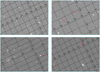 |
Fig. 1 Portions (approximately 1.′2 × 0.′9) of simulated VIS CCDs. The co-ordinate grid shows RA and Dec, while the red arrows indicate the SSO direction in the sky and have lengths proportional to the SSO velocity. From the upper left panel (in a clockwise direction), we show a few simulated objects in the magnitude bins 20–21, 22–23, 23–24, and 24–25, respectively. The SSO velocity is in the range of 0.″1–10″ h−1. Note that a small shift has been applied to each arrow to make the SSO streak behind it more evident. |
 |
Fig. 2 Simplified representation of the SSOFinder algorithm at work. A PIVOT source (orange dot in dither 1 panel) is considered a good SSO candidate if it appears to move in the remaining images (red dots in subsequent dithers) and all the tracklet members are on the same trajectory (see text). |
4 Purity and completeness of the detection tool
We assessed the behaviour of the SSO-PIPE pipeline by determining the purity and completeness of the output samples. In this respect, a sample was considered pure if objects detected as SSOs consisted of genuine simulated moving sources against the ‘detection background’ of stars, galaxies, and spurious features erroneously identified as SSOs by the algorithms. Therefore, we define (in each bin of width dυ centred at υ) the purity of the sample as
 (6)
(6)
where ND(v) is the number of objects detected as moving sources in each bin of velocity, and NDA(υ) is the number of genuine associations; that is, those objects identified as moving sources corresponding to real SSOs in the simulated input catalogue.
Similarly, the completeness of the output sample can be defined as the number of genuine associations, NDA(υ), over the number of all simulated SSOs, N(υ), in a particular velocity bin as
 (7)
(7)
so that, ideally, one would expect both purity and completeness close to unity for a perfect algorithm.
Of course, identifying a stationary source (star, galaxy, and spurious CCD artefact) as a SSO or assigning the detection to the wrong velocity bin (thus decreasing both purity and completeness) depends mainly on the random pixel noise, the CCD astrometric solution (that affects the low-velocity bins for faint objects), and the detection parameters, MIN_DIST and MAX_DIST, in SSOFinder, fixed here as 0.″04 and 12″ respectively. In particular, the MIN_DIST value was chosen as the typical astrometric accuracy in Euclid VIS images. On the other hand, a larger value of the MAX_DIST parameter resulted in many fake detections in the case of large velocity bins due to the faintness of the source.
After testing, we found a combination of parameters that appears to maximise the purity and completeness in the apparent motion range, 0.″1–10″ h−1, of the recovered SSO sample. There is a trade-off between maximising the number of SSO detections (true-positive targets) and minimising the number of fake moving sources recognised erroneously (false positives) by the pipeline.
In Figs. 3 and 4, we show the purity and completeness of the SSO sample recovered by the pipeline as a function of the asteroid’s apparent motion and for different magnitude bins. In the range of 1″–10″ h−1 (right panel), purity remains close to a 90% level for all the selected magnitude bins apart from the faintest one (25–26 mag), where, as is expected, it abruptly decreases to zero for SSOs with a velocity larger than 4″ h−1. On the other hand, completeness remains of the order of 80% for SSO speeds in the range of 1.″–10″ h−1 and for the brighter bins of magnitude, but it rapidly falls for higher velocities and fainter objects.
The main reason for the lower completeness of faster SSOs in the bins of higher magnitudes is that fast SSOs are fainter. Assuming a SSO with a magnitude of 25.5, the expected total count number in the IE band is approximately 610. For an assumed velocity of 5″ h−1 , the SSO produces only approximately 80 counts per pixel, which, for a zodiacal background as in Euclid Collaboration: Scaramella et al. (2022), corresponds to 4 σ over the background. Furthermore, a decrease in purity is also visible for velocities larger than 9″ h−1 and, on the other side of the inspected range in apparent motion, below 0.″4 h−1, a large decrease for all bins of magnitude comes up as well. In both cases, this is due to the intrinsic scatter that affects the centroid detection algorithm, which decreases the purity as more fake targets enter the sample.
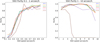 |
Fig. 3 Purity of the SSO sample recovered by the pipeline (see text for details) as a function of the object velocity and for different magnitude bins. Note that the purity abruptly decreases for the faintest SSOs (in the bin magnitude of 25–26) with an apparent motion faster than 4″ h−1. |
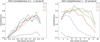 |
Fig. 4 Completeness of the SSO sample as a function of velocity and for different magnitude bins. |
5 Classification of Solar System objects based on self-organising maps
Once any detection tool is run on an image and a catalogue of SSO candidates is produced, one still needs to assess the quality of each candidate. Due to the large Euclid data volume, a visual inspection of each SSO candidate is impractical. Therefore, one must rely on a machine-learning approach to analyse the problem. In this respect, machine-learning techniques and neural networks have already proved to be very useful in astronomy with respect to, for example, the classification of different galaxy morphology types (Odewahn 1995; Dieleman et al. 2015), stellar spectra classification (Gulati et al. 1994), and the detection of strong gravitational lensing arcs (Schaefer et al. 2018). Lieu et al. (2019) trained deep CNNs on simulated VIS images to classify SSOs based on morphological properties. The CNNs were not used to detect the SSOs (a list of potential SSOs was, in fact, provided to the network, Lieu et al. 2019) but to reject false-positive detections. The CNNs separated the SSOs from other astronomical sources with an efficiency of 96% for apparent velocities larger than 10″ h−1 down to magnitude 26. Pöntinen et al. (2023) used a CNN to detect streaks and their co-ordinates in Euclid images and then a recurrent neural network to merge long streaks recognised as multiple targets by the previous step. The authors thus show the possibility of improving the detection efficiency of asteroid streaks using deep learning, especially for faint objects not detected by other methods.
With the ultimate goal of giving a classification for the objects detected by any deterministic algorithm (such as the one presented in the previous Sections, and for SSOs with velocities lower than 10″ h−1 down to magnitude 26), we present an algorithm designed to classify sources (stars, galaxies, and SSOs) based on their un-parameterised images. The method uses a form of neural network; namely, a SOM (Kohonen 1990). Due to the simplicity of the algorithm implementation and the capability to identify unknown features in the data, SOMs are widely used in astronomy; for example, in star and galaxy classification (Mähönen & Hakala 1995; Miller & Coe 1996), galaxy morphology classification (Naim et al. 1997; Molinari & Smareglia 1998), classification of gamma-ray bursts (Rajaniemi & Mähönen 2002), studies of mono-periodic light curves (Brett et al. 2004), and studies related to the calibration of photometric redshifts observed by Euclid (Masters et al. 2015; Euclid Collaboration: Saglia et al. 2022). We show here how to build an SOM architecture, train it, and extend its functionality to the classification of new data sets.
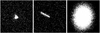 |
Fig. 5 Example of simulated star (left), SSO (middle), and galaxy (right). The data are normalised, as is described in the text. |
5.1 Preparing the data for self-organising-map training
In order to test the capability of an SOM to classify objects in an unsupervised fashion, we dealt with the simulation of thousands of different objects. In particular, to classify stars, galaxies, and SSOs, we concentrated on simulating stamps, each containing a specific source. We modelled each object of interest with a particular set of parameters such as the magnitude, luminosity profile, ellipticity, and position angle (for a galaxy), as well as velocity and direction of motion (for a moving SSO). We then built catalogues for training and testing the model (see Sects. 5.3–5.4). Each catalogue consists of 4000 random images in the form of 101 × 101-pixel matrices (suitable to host slow-moving SSOs), and the pixel size is that of a VIS image; that is, 0.″1 pixel−1.
Any particular image can host an object of the above type with stars and galaxies simulated with the Galsim software (Rowe et al. 2015). In particular, stellar objects were simulated as point-like sources, while galaxies were assumed to follow a Sérsic surface brightness profile characterised by three properties: the Sérsic index, n, the integrated flux (derived from the object magnitude, the VIS zero-point, and exposure time), and the half-light radius, re. For each galaxy, given these properties, the surface brightness profile scales with respect to r as
![Mathematical equation: $I(r) \propto \exp \left[ { - b{{\left( {r/{r_{\rm{e}}}} \right)}^{1/n}}} \right],$](/articles/aa/full_html/2025/02/aa51767-24/aa51767-24-eq9.png) (8)
(8)
where b is constrained to give the correct re value. Furthermore, each galaxy was deformed to account for an associated ellipticity and orientated in the sky according to a random position angle between 0 and 360 degrees. For each galaxy, we uniformly extracted a half-light radius in the range of 1.″–3.″(so that each stamp size is a factor of 2.5 larger than the maximum half-light diameter) and an ellipticity value between 0 and 0.8. The Sérsic index, n, was selected randomly in the range between 0.5 and 4, the latter corresponding to the de Vaucouleurs galaxy profile. The integrated galaxy magnitude was uniformly selected in the range of 14–24. It should be noted that training the neural network with galaxies that have Sérsic indices in the above range would allow one to correctly classify such objects (see Sect. 6.2 for a further discussion), but would fail for galaxies with different luminosity profiles and/or with more more complicated shapes, since the SOM noise enhances. Although the uniform distributions for the relevant parameters are unrealistic, this assumption is required to avoid biases during the SOM training phase and, furthermore, allows one to evaluate the completeness and purity of the classification regardless of the distribution details.
Once a star or a galaxy object has been simulated, the resulting image was then convolved with the VIS PSF and Poisson noise was added at a level of the noise expected in the data. Each stamp was also characterised by the same bias level (in counts per pixel) and a random read-out noise at a level of 3.5 counts per pixel. Knowing the exact value of the bias level is not crucial here, since each data set is first normalised before exposing the neural network to it.
We simulated the SSOs as a sequence of point-like objects (oversampling by a factor of ten to avoid PSF undersampling effects) and then convolved them with the instrumental PSF, as is described in Sect. 2. This procedure results in realistic SSO signatures in the simulated image. Also, in the case of the SSO simulation, we used the intrinsic features of the Galsim software to position the target onto the final image and for the PSF convolution. In Fig. 5, just as an example, we show a test data sample for a simulated star, SSO, and galaxy, respectively.
Finally, we stress again that, although Sérsic models reproduce the overall surface brightness of galaxies well (see e.g. Peng et al. 2002), the spatial resolution of the VIS images allows one to capture detailed features (such as bulges, spiral arms, and knots) in many of the observed galaxies, increasing the shape complexity. However, the increasing shape complexity acts against the object classification so that the intrinsic noise of the classifier would increase. We also remind the reader that the training sample is such that the relative weight among the simulated objects is equal. In other words, approximately a third of the training samples fall into each class of stars, SSOs, or galaxies. Since a Kohonen SOM classifies one image at a time, we require that each stamp contain only one specific object (for a similar case study, see e.g. Euclid Collaboration: Bretonnière et al. 2022). Object blending (images that might contain multiple categories amongst those searched for) increases the SOM noise against the target retrieval.
Quantifying the effects of resolved structures on the SOM image classifier as well as the impact of source blending on the SOM training and forecast is outside the purpose of the paper and will be investigated in future work. In any case, any SOM would need to be retrained with real Euclid data before offering reliable classifications of real detections.
5.2 Building a self-organising map
An SOM consists of a set of Q = N M neurons or nodes, typically organised in the form of a rectangular lattice. Each neuron of co-ordinates (i, j) (with i = 0,…, N − 1 and j = 0,…, M − 1) is characterised by a set of K values representing the components (k = 0,…, K − 1) of the ‘reference vector’ associated with that particular neuron. Each reference vector (with components rk) of the map is exposed to an input vector (each of which has components, wk, i.e. the same K cardinality as the reference vectors) taken from a training data set consisting of L inputs, such as images. The main purpose of the SOM training is to detect common patterns amongst the L inputs so that the data are ideally divided into well-separated groups. The number of Q neurons in the SOM follows from requiring that the resulting map not be too large to have one single neuron adapted per input data (the main goal is to generate clusters of similar data). Similarly, a map that is too poor fails to catch an adequate organisation of the data into separate classes. A common practice for a squared SOM (N = M) is to select a map size of  . We verified that a squared SOM with N = 20 neurons per side is sufficient to classify the data in our sample and to account for the appearance of stellar, galaxy, and SSO clusters in the map.
The SOM is trained by exposing all the neurons of the map iteratively to each sample in the training data set and by determining, for each sample, the associated winning neuron. We say that an ‘epoch’, t, passes when the SOM processes all the L inputs once. The final goal of training the network is to modify the values of the reference vector components so that the training samples that show some similarity are placed in nearby neurons. After each sample is associated with a node, the weights of the best winning neuron (and its close neighbours) are updated. The weight update continues until all the samples are passed to the SOM and the next epoch starts. Then, the entire procedure is repeated until the training members settle into (self-organised) clusters.
5.3 Determining the winning neuron
As is described above, the SOM is trained by passing, at a given epoch, t, the whole training set to the network, and determining, for each data sample, the best matching neuron minimising some distance function. A validation set is also passed to the neural network (see Sect. 5.4) to evaluate the SOM performance.
Here, the co-ordinates  of the winning node for an l-th input data sample (with l = 0,…, L − 1) are those obtained by minimising the Euclidean distance between the input vector and each reference vector [associated with the (i, j) pixel] in turn; that is, the quantity
 (9)
(9)
where the factor,  , is a mask that accounts for any missing value (or NaNs) in the input vector, l. In particular, by requiring that the mask equals one for any existing input vector component and zero otherwise (see e.g. Rejeb et al. 2022), the SOM algorithm can easily handle missing elements in the data sample.
Once a neuron of co-ordinates (i, j) has been flagged as the best matching node for an input sample, l, the k components (weights) of the node are updated together with the weights of close neurons according to the rule
 (10)
(10)
where ɑ(t/Ne) is the learning rate coefficient, H(t/Ne, d) is the neighbourhood updating function, and dwin and d indicate the vector positions of the best winning neuron and a nearby node, respectively. Here, we adopted a Gaussian function of the form
![Mathematical equation: $H\left( {t/{N_{\rm{e}}},{\bf{d}}} \right) = \exp \left\{ { - {d^2}/\left[ {2{\sigma ^2}\left( {t/{N_{\rm{e}}}} \right)} \right]} \right\}.$](/articles/aa/full_html/2025/02/aa51767-24/aa51767-24-eq15.png) (11)
(11)
The time co-ordinate, t, varies linearly with the epoch number, from t = 0 (at the first iteration) to t = Ne (Ne is the number of epochs). Moreover, the presence of a smooth neighbourhood kernel function, characterised by a variance σ2(t), enables the formation of clusters of nodes capable of catching similarities in the data.
The convergence of an SOM towards a stable configuration depends (at each epoch, t) on the learning rate, ɑ(t), which drives the blending of the reference vectors, and the σ(t) parameter, which affects the number of neurons (close to the winning node) whose weights are updated (according to Eqs. (10)–(11)) after each input sample is passed to the SOM. We studied the effects of varying ɑ(t) and σ(t) according to two possible different decreasing functions of time, t: a linearly decreasing monotonic function and an exponentially decreasing one. In the linear case, the functional form is
 (12)
(12)
Analogously, the exponentially decreasing function reads out to be
 (13)
(13)
where, in both cases, p(t) is either ɑ(t) or σ(t), and p0 gives the associated starting value of the involved quantity. In the exponential case, λ represents a scale parameter so that p(t) = 10−3p0 at the last iteration. The above scheme ensures that large-scale structures form in the map at a very early stage of the training procedure, and then they become stable (with little changes) at late epochs.
5.4 Monitoring the self-organising map and early stopping of the training
The learning behaviour of the SOM can be evaluated by using a statistic indicating the difference between the input samples (input vectors) and the reference vectors associated with each neuron. At each epoch, we evaluated the minimum distance between a sample and the associated winning neuron reference vector (see Eq. (9)) averaged over all members of the training set as
 (14)
(14)
We expect that the SOM error, S (t), turns out to be relatively large at the early stages of the training process and decreases as the number of iterations increases. After the SOM changes the learning rate and variance values (α(t) and σ(t), respectively), it reaches a stable condition, and the average error shows a slower decline. We also expect that, during the initial epochs, the training samples jump in the SOM map so that the winning neuron changes with time. Once the SOM becomes stable, the number of jumps decreases as clusters of similar data form. Therefore, we can define (in analogy to Brett et al. 2004) a second measure of the SOM quality; namely, Nmove , which consists of counting the number of training set members that have changed locations on the map in each epoch. We expect that Nmove is very large at the beginning of the training, because we assigned all the data members to a virtual neuron outside the SOM map. Therefore, in the first epoch, all L members jump to a new position and Nmove = L. The number of movements then decreases, reaches a maximum (at the stage of maximum learning), and then approaches zero when all the clusters of similar patterns have formed.
From the SOM training scheme described above, it should be clear that Ne can be set to a large number, implying a very long, time-consuming procedure. A second effect is that iterating the training over the same data pushes the SOM to an over-fitting state so that the SOM error S (t) decreases (eventually becoming constant when Nmove approaches zero) and all the weights are exactly adapted to the particular set under examination, but do not generalise for other data.
Therefore, with the training scheme of the SOM, we decided to implement an ‘early stopping’ method consisting of training the neural network on the input data set and checking the quality of the SOM by evaluating S (t) and Nmove at each step, but also testing its performance on an independent, randomly chosen validation data set. We then evaluated the SOM error, Sval(t), for the validation data and compared it with the SOM error under training. The idea behind the early stopping method is that over the epochs, S(t) and Sval(t) both decrease, and when the over-fitting stage is reached, Sval(t) shows a minimum and then flattens or starts to increase. We flag this stage as the tover−fitting epoch, stop the learning process, and freeze the weights stored in each neuron. Once trained in this way, the SOM acquires the capability to classify new data.
5.5 U-matrix associated with the trained self-organising map
When the training process of the SOM has been completed, the map can be inspected and searched for clusters of similar neurons. This can be done, for example, by studying the distribution of the training set members that fall on a given node. Here, we prefer to adopt the approach described in Ultsch & Siemon (1990), calculating the U-matrix associated with the SOM. A U-matrix simply evaluates the rate of change in the neuron response (the reference vector) across the SOM so that neurons belonging to the same cluster have similar reference vector components, while at the boundaries among clusters, the differences increase. Therefore, for each neuron of the map, we calculate the quantity
 (15)
(15)
where, when possible, the eight nearest neighbours of the neuron under investigation are averaged.
6 Application of an SOM to the classification of stars, galaxies, and Solar System objects
6.1 Training the self-organising map
In Sect. 5.1, we described the method adopted to simulate a sample of image data corresponding to point-like stars, galaxies, and SSOs, a few examples of which are given in Fig. 5. Each image, simulated initially as a 101 × 101-pixel matrix, is first rebinned by a factor of f = 3, so that enough details are available for the SOM to determine common patterns, and then normalised to unit variance. Following the training scheme outlined in Sect. 5.2, we found that a map of 20 × 20 neurons was capable of autonomously identifying clusters for the three classes of objects hidden in the training data.
We fixed the starting value of the dispersion parameter, σ(t), to four, allowing the SOM to form large clusters at the beginning of the iterations. We tested the behaviour of the network for two initial values of the learning parameter, α(t), namely 0.1 and 0.5, and for each combination of parameters we trained the SOM by assuming the linear or the exponential functions (see Eqs. (12)–(13)). We always set Ne = 500, and by passing each data sample to the SOM, the winning neuron was identified and the map weights updated.
In each epoch (once the SOM was exposed to the entire data set), we monitored the performance of the neural network (as is described in Sect. 5.4) and updated the values of σ(t) and α(t). Consequently, the early-stopping method prevented the SOM from over-fitting to the input data.
In the proposed scheme, the 20 × 20 neurons’ reference vectors should be initialised by picking random data from the training set. To test the neural network performance, we always initialised the map with the same weights and selected a combination of starting values for σ(t) and α(t), and selected one decreasing function between Eqs. (12) and (13).
In Fig. 6, we show the performance of the neural network by evaluating the error, S (t), and the number of movements, Nmove (t), at any epoch, t. In the left panels, the orange line gives the error, Sval(t), evaluated by applying the SOM on a validation data set in order to identify the over-fitting epoch (see Sect. 5.4 for details), which is flagged by the vertical dashed line. In the first and second rows, the SOM was trained by assuming a starting learning parameter, α = 0.1, and adopting a linear and exponential decreasing function, respectively. Analogously, in the third and fourth rows, we used α = 0.5 and again tested the network behaviour with the two adopted decay functions.
As is evident from Fig. 6, the result does not depend critically on the starting value of the learning parameter nor the adopted form of the decreasing function. At the end of the last epoch, the training of the SOM with the input data reaches a stable configuration characterised by errors of the same order of magnitude for all runs.
For any starting α parameter, the left panels show a monotonic improvement (decrease) in the error statistic, S(t), which corresponds to a decrease in the σ(t) value. During this phase, the SOM organises itself and finds clusters of similar data until it reaches a steady state at the end of the learning procedure. This is also reflected in the right panels where, for each selected pair of the α starting value and decreasing function, the Nmove statistic is given. As was expected, the number of samples that change location in the map is large in the early stages of the training when the SOM is still creating large clusters, and then approaches zero, which indicates few movements during the fine-tuning of the weights or no movement at all, when the SOM has been trained.
We note that Nmove depends on the starting value of the learning parameter, α. In particular, for α = 0.1 and α = 0.5, when adopting a linear decreasing function, the clusters continue to move around the map (Nmove remains relatively large) until the SOM stabilises. Although the SOM converges on practically the same error, large movements at all epochs are unlikely in a real application. Therefore, we prefer the behaviour of the SOM trained by using the exponential decaying function (second and fourth rows in Fig. 6). In this respect, the application of the early- stopping method implies that a general SOM becomes organised enough to classify new data after approximately 150 epochs, and we prefer the SOM decaying as an exponential with α = 0.5, because of its slightly smaller error reached when classifying the test data.
After selecting the SOM architecture, we started training on the input data again with early stopping, as was discussed before, but this time allowing (for each run) a different initialisation of the neuron weights. We then selected the SOM with the smallest error in the epoch of over-fitting, tover–fitting.
Finally, we built the associated U-matrix and projected onto each pixel the members of the input data set for which we had an a priori classification. Figure 7 shows the 20 × 20 U-matrix superimposed with a different symbol and colour for each type of input vector (stars, galaxies, and SSOs), showing that the SOM succeeded in classifying the data correctly. The co-ordinates of the objects falling in the same neuron have been randomised within the same pixel for graphical purposes. In this respect, we note that the SSOs (red circles) that fall in the SOM region prevalently associated with stars (blue circles) are slow-speed objects that appear as point sources (characterised by a velocity below 1″ h−1) so that the SOM hardly separates them from the rest of classes. A further inspection of the same figure reveals that SSOs are spread over a large map area. This occurs since the neural network autonomously clusters the SSOs with similar lengths and orientations in the training images. Analogously, the SOM organises the galaxies, spreading them depending on the size and shape, placing those characterised by a large ellipticity at the outskirts of the long SSO region, as expected. In Fig. 8, we give the results of the trained SOM exposed to a new test data set consisting of 2000 images with stars, galaxies, and SSOs for which we already have an a priori classification. As can be seen from the superimposed objects, the early-stopped SOM can adequately classify the new data. The underlying grey-scale image represents the U-matrix associated with the trained SOM.
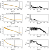 |
Fig. 6 Performance of the SOM evaluated by calculating the average map error, S (t) (solid black line, left panels), and number of movements, Nmove(t), in a given epoch, t (right panels). In the left panels, we also give the average error of the SOM when applied to the validation input data (yellow line). The dashed vertical lines represent, for each panel, the epoch associated with the early-stopping method (see text for details). |
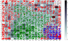 |
Fig. 7 20 × 20 U-matrix of the SOM trained to classify stars, galaxies, and SSOs. Using the training data, we superimposed a different symbol and colour in the middle of each node for each type of input vector (blue circles for stars, green squares for galaxies, and red diamonds for SSOs), confirming that the SOM correctly classified the data. The dots appearing in each pixel (with a different colour for each class) indicate the number of objects of the particular class classified by the SOM. The underlying grey-scale image represents the U-matrix associated with the trained SOM, while numbers along the axes represent the neuron position in the map. |
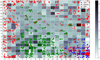 |
Fig. 8 20 × 20 U-matrix of the same SOM given in Fig. 7 but exposed to a test data set. Having the correct class of the test data, we flagged the objects falling in each neuron with a different symbol and colour, and thus confirmed the capability of the (early stopped) SOM to classify a new data set. The meaning of the symbols and colours is as described in Fig. 7. |
6.2 Self-organising-map probability
Since our final goal is to apply the trained SOM to a new data set (for which, of course, no a priori classification is given), we can associate with the neural network a probability of having an object type (picked up from a particular data set, x) in a given map neuron. This probability,  is simply given by the ratio between the number of objects of a particular class falling in a neuron and the total number of test samples found in the same neuron, regardless of the associated type, as
 (16)
(16)
where the class can be either star, galaxy, or SSO.
Although the general behaviour of the trained SOM is fixed, the probability, as is defined above, might be characterised by fluctuations depending on the data set passed to the neural network. Therefore, we simulated X = 30 data sets (each of which contains 2000 different objects), required that every class be represented by approximately 1/3 of the sample number, and gave the data sets to the SOM for a blind classification. For each data set, we then evaluated the probability per node for a given class,  , and then averaged the results over the number, X, of data sets; in other words,
 (17)
(17)
The results of the above calculation are reported in Figs. 9, 10, and 11, where we give the probability that the SOM classifies input data into the SSO, star, and galaxy classes, respectively. The maps are normalised so that summing the class probabilities gives exactly 100%.
The usefulness of such maps is evident when trying to classify new input data with the trained SOM. In particular, when data is injected into the SOM and a winning node is identified, the probability per class associated with that neuron can be retrieved. We found that, although a trained SOM is capable of correctly classifying new images containing stars, SSOs, and galaxies with a certain degree of accuracy, SSOs characterised by a very slow speed (namely below 1″ h−1 ) are visually indistinguishable from point-like stars, and the SOM fails to classify them correctly. This is also clear from the classification map given in Fig. 8, where star versus SSO confusion appears in the bottom right corner of the SOM.
The final recipe for determining the detection quality turns out to be:
For each source detected as a SSO by the SSO-PIPE pipeline (see Sect. 3), an image of 101 × 101 pixels (centred on the target co-ordinates) is extracted. The image is then rebinned by a factor of three so that its cardinality is K.
By using the trained SOM (with N = M = 20 per side), a winning node (characterised by k components) is identified for any input image.
The probability maps in Figs. 9, 10, and 11 are then queried at the winning neuron co-ordinates, and the probability (per class) is extracted. This probability is then interpreted as the quality flag associated with the input target. Alternatively, a given input object is associated with the classification corresponding to the largest extracted probability.
To assess the overall quality of the SOM, we followed the previous recipe and fed the SOM with a fresh validation set consisting of 104 images (each including one amongst stars, galaxies, and SSOs simulated as is described in Sect. 2 and with a priori knowledge of the classification). We then evaluated the behaviour of the neural network by calculating the purity and completeness of the results (see Eqs. (6)–(7)) as a function of the SSO speed but regardless of the object magnitude. For simplicity, we explicitly considered three bins of velocity (namely, 0″–3″ h−1, 3″–6″ h−1, and 6″–10″ h−1) and found purity (completeness) values of 15% (70%), 100% (60%), and 100% (58%) in the first, second, and third bins, respectively. This behaviour is expected, since SSOs with velocity values that fall in the first bin (and in particular those with velocity smaller than 0.″5 h−1) are not correctly recognised by the SOM but misclassified as stars, being formally indistinguishable from a fixed point-like source in a single image.
 |
Fig. 9 SSO probability map (for a 20 × 20 SOM) associated with the trained neural network (see text for details). The value of each pixel (according to the associated colour bar) gives the normalised probability that the data falling in that particular neuron belongs to the SSO class. The probability is normalised so that by summing up the probability per class, one gets exactly 100%. |
7 Results and discussion
In this paper, we describe the main features of the <MONO>SSO-PIPE</MONO>, a software developed and maintained at the Euclid Science Operation Centre in ESAC/ESA, dedicated to the detection (and classification) of slow-moving SSOs with typical speeds lower than 10″ h−1 in Euclid VIS images.
SSO-PIPE shows high efficiency in recognising SSOs, particularly within the speed range of 0.″5–9″ h−1 and in magnitude bins where sources appear brighter, specifically up to 24–25 in magnitude. Analysing the simulated observations with 2000 SSOs per field returns an approximate probability of 80% of detecting a moving object. The probability that a detected object is a genuine SSO can be as large as 90%, indicating a high purity level. However, detecting fainter objects (falling in the last bin of investigated magnitude, 25–26) fails in most cases. This is particularly true for faster objects characterised by very elongated streaks, which tend to blend into the background. Furthermore, as is seen in Figs. 3 and 4, the detection and recognition of high-speed objects, specifically those approaching the 10″ h−1 limit, shows a decay due to inaccurate estimates of the target co-ordinates caused by the source fragmentation. This fact leads to a failure to detect objects whose velocity and position angle accuracy do not fall in the corresponding uncertainty limits considered in the pipeline. Conversely, detecting objects with speeds <0.″5 h−1 is challenging, since very slow-moving objects appear almost stationary and are therefore confused with stars.
In this paper, we have also tested the possibility of using an SOM to separate the observed objects into star, galaxy, and SSO classes. Working on simulated data, we have shown that an SOM can be used as a classifier for new data sets if trained with the early-stopping technique. The SOM can recognise SSOs on realistic simulated images with relatively high accuracy, provided the object has a speed higher than 1″ h−1 . Below this value, the neural network becomes practically useless in classifying the examined object, which appears formally indistinguishable from a fixed point-like source in a single image.
We have also verified that the SOM, if correctly trained, can disentangle between point-like stars and galaxies. In particular, as is implemented in this work, the trained SOM is capable of correctly classifying galaxies when characterised by a Sérsic index in the range of 0.5–4. Contrarily, any increasing shape complexity introduces noise into the classification. As a matter of fact, there is always at least a difference between simulated and authentic images, and therefore, to work optimally with real Euclid data, the SOM probably requires retraining with a new training set consisting partially or entirely of real training examples. Furthermore, the SOM is a particular neural network that recognises one pattern at a time. Therefore, under the assumption that the SOM is fed with an image containing multiple objects (for example, two sources belonging to different classes), the neural network will interpret the input as a particular noisy example of one class, with the non-retrieved object as a source of noise for the recognised one. Investigating the source blending in the SOM training and forecasting remains work for the future.
Finally it is worth noting that this approach for the detection and classification of SSOs in true Euclid VIS images (acquired during the week-long Phase Diversity Calibration campaign specifically planned towards the ecliptic for Solar System science) is currently in progress. This involves accurate fine tuning of all the detection parameters as well as retraining the presented neural network with real cases.
Acknowledgements
We are grateful for support from the ESAC (ESA) Science faculty and the INFN projects TAsP and EUCLID. This work is (partially) supported by ICSC – Centro Nazionale di Ricerca in High Performance Computing, Big Data and Quantum Computing, funded by European Union -– NextGenerationEU. The authors acknowledge the Euclid Consortium, the European Space Agency, and a number of agencies and institutes that have supported the development of Euclid, in particular the Agenzia Spaziale Italiana, the Austrian Forschungsförderungsgesellschaft funded through BMK, the Belgian Science Policy, the Canadian Euclid Consortium, the Deutsches Zentrum für Luft- und Raumfahrt, the DTU Space and the Niels Bohr Institute in Denmark, the French Centre National d’Etudes Spatiales, the Fundação para a Ciência e a Tecnologia, the Hungarian Academy of Sciences, the Ministerio de Ciencia, Innovación y Universidades, the National Aeronautics and Space Administration, the National Astronomical Observatory of Japan, the Netherlandse Onderzoekschool Voor Astronomie, the Norwegian Space Agency, the Research Council of Finland, the Romanian Space Agency, the State Secretariat for Education, Research, and Innovation (SERI) at the Swiss Space Office (SSO), and the United Kingdom Space Agency. A complete and detailed list is available on the Euclid web site (www.euclid-ec.org).
References
- Bertin, E., & Arnouts, S. 1996, A&AS, 117, 393 [NASA ADS] [CrossRef] [EDP Sciences] [Google Scholar]
- Bertin, E. 2006, in Astronomical Society of the Pacific Conference Series, 351, Astronomical Data Analysis Software and Systems XV, eds. C. Gabriel, C. Arviset, D. Ponz, & S. Enrique, 112 [NASA ADS] [Google Scholar]
- Bouy, H., Bertin, E., Moraux, E., et al. 2013, A&A, 554, A101 [NASA ADS] [CrossRef] [EDP Sciences] [Google Scholar]
- Brett, D. R., West, R. G., & Wheatley, P. J. 2004, MNRAS, 353, 369 [CrossRef] [Google Scholar]
- Carruba, V., & Machuca, J. F. 2011, MNRAS, 418, 1102 [CrossRef] [Google Scholar]
- Carry, B. 2018, A&A, 609, A113 [NASA ADS] [CrossRef] [EDP Sciences] [Google Scholar]
- Chambers, K., & Pan-STARRS Team 2018, in American Astronomical Society Meeting Abstracts, 231, 102.01 [NASA ADS] [Google Scholar]
- Chen, Y.-T., Lin, H. W., Holman, M. J., et al. 2016, ApJ, 827, L24 [Google Scholar]
- Deienno, R., Gomes, R. S., Walsh, K. J., Morbidelli, A., & Nesvorný, D. 2016, Icarus, 272, 114 [CrossRef] [Google Scholar]
- DeMeo, F., Binzel, R. P., Slivan, S. M., & Bus, S. J. 2009, Icarus, 202, 160 [NASA ADS] [CrossRef] [Google Scholar]
- Dieleman, S., Willett, K. W., & Dambre, J. 2015, MNRAS, 450, 1441 [NASA ADS] [CrossRef] [Google Scholar]
- Durech, J., Carry, B., Delbo, M., Kaasalainen, M., & Viikinkoski, M. 2015, Asteroid Models from Multiple Data Sources (University Arizona Press), 183 [Google Scholar]
- Eggl, S. 2011, Celest. Mech. Dyn. Astron., 109, 211 [NASA ADS] [CrossRef] [Google Scholar]
- Euclid Collaboration (Bretonnière, H., et al.) 2022, A&A, 657, A90 [CrossRef] [EDP Sciences] [Google Scholar]
- Euclid Collaboration (Saglia, R., et al.) 2022, A&A, 664, A196 [NASA ADS] [CrossRef] [EDP Sciences] [Google Scholar]
- Euclid Collaboration (Scaramella, R., et al.) 2022, A&A, 662, A112 [NASA ADS] [CrossRef] [EDP Sciences] [Google Scholar]
- Euclid Collaboration (Schirmer, M., et al.) 2022, A&A, 662, A92 [NASA ADS] [CrossRef] [EDP Sciences] [Google Scholar]
- Euclid Collaboration (Cropper, M., et al.) 2024, https://doi.org/10.1051/0004-6361/202450996 [Google Scholar]
- Euclid Collaboration (Jahnke, K., et al.) 2024, https://doi.org/10.1051/0004-6361/202450786 [Google Scholar]
- Euclid Collaboration (Mellier, Y., et al.) 2024, https://doi.org/10.1051/0004-6361/202450810 [Google Scholar]
- Euclid Collaboration (Serrano, S., et al.) 2024, A&A, 690, A103 [NASA ADS] [CrossRef] [EDP Sciences] [Google Scholar]
- Gaia Collaboration (Brown, A. G. A., et al.) 2018a, A&A, 616, A1 [NASA ADS] [CrossRef] [EDP Sciences] [Google Scholar]
- Gaia Collaboration (Spoto, F., et al.) 2018b, A&A, 616, A13 [NASA ADS] [CrossRef] [EDP Sciences] [Google Scholar]
- Gaia Collaboration (Vallenari, A., et al.) 2023, A&A, 674, A1 [NASA ADS] [CrossRef] [EDP Sciences] [Google Scholar]
- Granvik, M., Muinonen, K., Jones, L., et al. 2007, Icarus, 192, 475 [Google Scholar]
- Gulati, R. K., Gupta, R., Gothoskar, P., & Khobragade, S. 1994, ApJ, 426, 340 [CrossRef] [Google Scholar]
- Hildebrandt, H., Viola, M., Heymans, C., et al. 2017, MNRAS, 465, 1454 [Google Scholar]
- Ivezić, Ž., Kahn, S. M., Tyson, J. A., et al. 2019, ApJ, 873, 111 [Google Scholar]
- Kohonen, T. 1990, Proc. IEEE, 78, 1464 [Google Scholar]
- Kohonen, T. 2001, Self-organizing Maps, 3rd edn. (Springer Berlin, Heidelberg) [CrossRef] [Google Scholar]
- Lang, D., Hogg, D. W., Mierle, K., Blanton, M., & Roweis, S. 2010, AJ, 139, 1782 [Google Scholar]
- Laureijs, R., Amiaux, J., Arduini, S., et al. 2011, arXiv e-prints [arXiv:1110.3193] [Google Scholar]
- Lieu, M., Conversi, L., Altieri, B., & Carry, B. 2019, MNRAS, 485, 5831 [NASA ADS] [CrossRef] [Google Scholar]
- Maciaszek, T., Ealet, A., Jahnke, K., et al. 2014, SPIE, 9143, 91430K [NASA ADS] [Google Scholar]
- Maciaszek, T., Ealet, A., Jahnke, K., et al. 2016, SPIE Conf. Ser., 9904, 99040T [NASA ADS] [Google Scholar]
- Mahlke, M., Bouy, H., Altieri, B., et al. 2018, A&A, 610, A21 [NASA ADS] [CrossRef] [EDP Sciences] [Google Scholar]
- Mähönen, P. H., & Hakala, P. J. 1995, ApJ, 452, L77 [NASA ADS] [Google Scholar]
- Masters, D., Capak, P., Stern, D., et al. 2015, ApJ, 813, 53 [Google Scholar]
- Miller, A. S., & Coe, M. J. 1996, MNRAS, 279, 293 [NASA ADS] [CrossRef] [Google Scholar]
- Molinari, E., & Smareglia, R. 1998, A&A, 330, 447 [NASA ADS] [Google Scholar]
- Nagasawa, M., Ida, S., & Tanaka, H. 2001, Earth Planets Space, 53, 1085 [Google Scholar]
- Naim, A., Ratnatunga, K. U., & Griffiths, R. E. 1997, ApJS, 111, 357 [NASA ADS] [CrossRef] [Google Scholar]
- Namouni, F., & Morais, M. H. M. 2020, MNRAS, 494, 2191 [Google Scholar]
- Novaković, B., Cellino, A., & Kneževic, Z. 2011, Icarus, 216, 69 [CrossRef] [Google Scholar]
- Odewahn, S. C. 1995, PASP, 107, 770 [Google Scholar]
- Peng, C. Y., Ho, L. C., Impey, C. D., & Rix, H.-W. 2002, AJ, 124, 266 [Google Scholar]
- Pöntinen, M., Granvik, M., Nucita, A. A., et al. 2020, A&A, 644, A35 [NASA ADS] [CrossRef] [EDP Sciences] [Google Scholar]
- Pöntinen, M., Granvik, M., Nucita, A. A., et al. 2023, A&A, 679, A135 [NASA ADS] [CrossRef] [EDP Sciences] [Google Scholar]
- Popescu, M., Licandro, J., Carvano, J. M., et al. 2018, A&A, 617, A12 [NASA ADS] [CrossRef] [EDP Sciences] [Google Scholar]
- Prieto, E., Amiaux, J., Auguères, J.-L., et al. 2012, SPIE Conf. Ser., 8442, 84420W [NASA ADS] [Google Scholar]
- Racca, G. D., Laureijs, R., Stagnaro, L., et al. 2016, in Space Telescopes and Instrumentation 2016: Optical, Infrared, and Millimeter Wave, 9904, eds. H. A. MacEwen, G. G. Fazio, M. Lystrup, N. Batalha, N. Siegler, & E. C. Tong, International Society for Optics and Photonics (SPIE), 99040O [Google Scholar]
- Rajaniemi, H. J., & Mähönen, P. 2002, ApJ, 566, 202 [NASA ADS] [CrossRef] [Google Scholar]
- Rejeb, S., Duveau, C., & Rebafka, T. 2022, arXiv e-prints [arXiv:2202.07963] [Google Scholar]
- Rhodes, J., Nichol, R. C., Aubourg, É., et al. 2017, ApJS, 233, 21 [Google Scholar]
- Rowe, B., Jarvis, M., Mandelbaum, R., et al. 2015, Astron. Comput., 10, 29 [Google Scholar]
- Schaefer, C., Geiger, M., Kuntzer, T., & Kneib, J. P. 2018, A&A, 611, A2 [NASA ADS] [CrossRef] [EDP Sciences] [Google Scholar]
- Schlafly, E. F., Meisner, A. M., & Green, G. M. 2019, ApJS, 240, 30 [Google Scholar]
- Shannon, A., Jackson, A. P., & Wyatt, M. C. 2019, MNRAS, 485, 5511 [CrossRef] [Google Scholar]
- Snodgrass, C., Carry, B., Berthier, J., et al. 2018, arXiv e-prints [arXiv:1812.00607] [Google Scholar]
- Terai, T., & Itoh, Y. 2011, PASJ, 63, 335 [NASA ADS] [CrossRef] [Google Scholar]
- Tsiganis, K., Gomes, R., Morbidelli, A., & Levison, H. F. 2005, Nature, 435, 459 [Google Scholar]
- Ultsch, A., & Siemon, H. P. 1990, in Proceedings of the International Neural Network Conference (INNC-90), Paris, France, July 9–13, 1990, Dordrecht, Netherlands, 1, eds. B. Widrow, & B. Angeniol (Dordrecht, Netherlands: Kluwer Academic Press), 305 [Google Scholar]
- van Dokkum, P. G. 2001, PASP, 113, 1420 [Google Scholar]
- Virtanen, J., Poikonen, J., Säntti, T., et al. 2016, Adv. Space Res., 57, 1607 [NASA ADS] [CrossRef] [Google Scholar]
- Walsh, K. J., Morbidelli, A., Raymond, S. N., O’Brien, D. P., & Mandell, A. M. 2011, Nature, 475, 206 [Google Scholar]
A similar method based on SExtractorand SCAMP is described in Bouy et al. (2013) and Mahlke et al. (2018) when searching for sources at different positions in dithered images as those provided by the Kilo-Degree Survey (http://kids.strw.leidenuniv.nl).
All Figures
|
Fig. 1 Portions (approximately 1.′2 × 0.′9) of simulated VIS CCDs. The co-ordinate grid shows RA and Dec, while the red arrows indicate the SSO direction in the sky and have lengths proportional to the SSO velocity. From the upper left panel (in a clockwise direction), we show a few simulated objects in the magnitude bins 20–21, 22–23, 23–24, and 24–25, respectively. The SSO velocity is in the range of 0.″1–10″ h−1. Note that a small shift has been applied to each arrow to make the SSO streak behind it more evident. |
| In the text | |
|
Fig. 2 Simplified representation of the SSOFinder algorithm at work. A PIVOT source (orange dot in dither 1 panel) is considered a good SSO candidate if it appears to move in the remaining images (red dots in subsequent dithers) and all the tracklet members are on the same trajectory (see text). |
| In the text | |
|
Fig. 3 Purity of the SSO sample recovered by the pipeline (see text for details) as a function of the object velocity and for different magnitude bins. Note that the purity abruptly decreases for the faintest SSOs (in the bin magnitude of 25–26) with an apparent motion faster than 4″ h−1. |
| In the text | |
|
Fig. 4 Completeness of the SSO sample as a function of velocity and for different magnitude bins. |
| In the text | |
|
Fig. 5 Example of simulated star (left), SSO (middle), and galaxy (right). The data are normalised, as is described in the text. |
| In the text | |
|
Fig. 6 Performance of the SOM evaluated by calculating the average map error, S (t) (solid black line, left panels), and number of movements, Nmove(t), in a given epoch, t (right panels). In the left panels, we also give the average error of the SOM when applied to the validation input data (yellow line). The dashed vertical lines represent, for each panel, the epoch associated with the early-stopping method (see text for details). |
| In the text | |
|
Fig. 7 20 × 20 U-matrix of the SOM trained to classify stars, galaxies, and SSOs. Using the training data, we superimposed a different symbol and colour in the middle of each node for each type of input vector (blue circles for stars, green squares for galaxies, and red diamonds for SSOs), confirming that the SOM correctly classified the data. The dots appearing in each pixel (with a different colour for each class) indicate the number of objects of the particular class classified by the SOM. The underlying grey-scale image represents the U-matrix associated with the trained SOM, while numbers along the axes represent the neuron position in the map. |
| In the text | |
|
Fig. 8 20 × 20 U-matrix of the same SOM given in Fig. 7 but exposed to a test data set. Having the correct class of the test data, we flagged the objects falling in each neuron with a different symbol and colour, and thus confirmed the capability of the (early stopped) SOM to classify a new data set. The meaning of the symbols and colours is as described in Fig. 7. |
| In the text | |
|
Fig. 9 SSO probability map (for a 20 × 20 SOM) associated with the trained neural network (see text for details). The value of each pixel (according to the associated colour bar) gives the normalised probability that the data falling in that particular neuron belongs to the SSO class. The probability is normalised so that by summing up the probability per class, one gets exactly 100%. |
| In the text | |
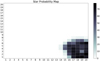 |
Fig. 10 Same as in Fig. 9 but for the star class. |
| In the text | |
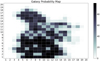 |
Fig. 11 Same as in Fig. 9 but for the galaxy class. |
| In the text | |
Current usage metrics show cumulative count of Article Views (full-text article views including HTML views, PDF and ePub downloads, according to the available data) and Abstracts Views on Vision4Press platform.
Data correspond to usage on the plateform after 2015. The current usage metrics is available 48-96 hours after online publication and is updated daily on week days.
Initial download of the metrics may take a while.