| Issue |
A&A
Volume 693, January 2025
|
|
|---|---|---|
| Article Number | L10 | |
| Number of page(s) | 10 | |
| Section | Letters to the Editor | |
| DOI | https://doi.org/10.1051/0004-6361/202452622 | |
| Published online | 08 January 2025 | |
Letter to the Editor
The IACOB project
XIII. Helium enrichment in O-type stars as a tracer of past binary interaction
1
Instituto de Astrofísica de Canarias, c/Vía Láctea, s/n, E-38205 La Laguna, Tenerife, Spain
2
Departamento de Astrofísica, Universidad de La Laguna, E-38206 La Laguna, Tenerife, Spain
3
Argelander Institut für Astronomie, Auf dem Hügel 71, DE-53121 Bonn, Germany
4
Center for Computational Astrophysics, Division of Science, National Astronomical Observatory of Japan, 2-21-1, Osawa, Mitaka, Tokyo, 181-8588, Japan
5
Max-Planck-Institut für Radioastronomie, Auf dem Hügel 69, DE-53121 Bonn, Germany
6
LMU Munich, Universitätssternwarte, Scheinerstrasse 1, 81679 München, Germany
⋆ Corresponding author; This email address is being protected from spambots. You need JavaScript enabled to view it.
Received:
15
October
2024
Accepted:
18
December
2024
Abstract
There is increasing evidence that single-star evolutionary models are unable to reproduce all of the observational properties of massive stars. Binary interaction has emerged as a key factor in the evolution of a significant fraction of massive stars. In this study, we investigate the helium (YHe) and nitrogen (ϵN) surface abundances in a comprehensive sample of 180 Galactic O-type stars with projected rotational velocities of ≤150 km s−1. We found a subsample (∼20% of the total, and ∼80% of the stars with YHe ≥ 0.12) with a YHe and ϵN combined pattern that is unexplainable by single-star evolution. We argue that the stars with anomalous surface abundance patterns are binary interaction products.
Key words: stars: abundances / stars: atmospheres / binaries: general / stars: evolution / stars: massive
© The Authors 2025
 Open Access article, published by EDP Sciences, under the terms of the Creative Commons Attribution License (https://creativecommons.org/licenses/by/4.0), which permits unrestricted use, distribution, and reproduction in any medium, provided the original work is properly cited.
This article is published in open access under the Subscribe to Open model. This email address is being protected from spambots. You need JavaScript enabled to view it. to support open access publication.
1. Introduction
Since the early 1970s, the reliable interpretation of surface abundance patterns of CNO-cycle products in main sequence (MS) O- and B-type stars has remained challenging. According to the standard theory of stellar structure and evolution, non-rotating massive stars do not bring nuclear-processed matter to their outermost radiative layers during the MS. Therefore, the composition of the stellar surface should mirror the initial abundances. However, for more than five decades, there has been clear and continuously increasing observational evidence of enhanced helium (He) and nitrogen (N) abundances in the photospheres of a significant number of these stars (see, e.g., Lester 1973; Schonberner et al. 1988; Herrero et al. 1992; Lyubimkov 1996; Howarth & Smith 2001; Morel et al. 2006; Hunter et al. 2008, 2009; Rivero González et al. 2012; Bouret et al. 2013, 2021; Martins et al. 2015, 2017, 2024; Markova et al. 2018; Grin et al. 2017; Carneiro et al. 2019).
Internal mixing processes induced by stellar rotation were initially proposed as a robust theoretical explanation for the observed abundances (see review by Maeder & Meynet 2000). However, new observations from spectroscopic surveys soon began to reveal certain limitations of this scenario (e.g., Hunter et al. 2008, 2009; Brott et al. 2011), highlighting the need for additional physical mechanisms to explain the occurrence of contaminated stellar surfaces. At this juncture, it was proposed that mass transfer and merging events in binary systems could play an important role (see, e.g., Langer 2012, and references therein), with complementary studies arguing in favor of a potential contribution from internal gravity waves (Aerts et al. 2014). Also, the properties of a distinct subpopulation seem to be best explained via magnetic stellar evolution models (e.g., Potter et al. 2012; Keszthelyi et al. 2019, 2022; Takahashi & Langer 2021).
Since then, many objects previously thought to be single stars have been discovered to be part of binary or even higher-order multiple systems (e.g., Sana et al. 2014; Aldoretta et al. 2015; Barbá et al. 2017; Maíz Apellániz et al. 2019). Furthermore, the majority of massive stars have been claimed to undergo interaction processes throughout their lifetime (Sana et al. 2012). Consequently, a rich set of post-interaction products are expected to be formed (such as stripped stars, rapidly rotating accretors, or merger stars; see review by Marchant & Bodensteiner 2024), broadening the spectrum of the observational cases to be interpreted.
The increasing availability of high-quality spectroscopic observations of massive stars (e.g., Evans et al. 2005, 2011; Simón-Díaz et al. 2011, 2020; Maíz Apellániz et al. 2020; Villaseñor et al. 2021; Shenar et al. 2024) allows a more comprehensive study, improving parameter coverage and enhancing statistical significance. This advancement enables more efficient identification of specific subsamples, which can be used to better understand and constrain the various proposed physical mechanisms leading to contaminated surfaces in massive MS stars. With this Letter, we present a demonstration of this powerful approach. We provide strong empirical evidence of the identification of a specific subset of 36 Galactic O-type stars (from within a sample of 180 targets) whose surface abundance pattern of He and N cannot be produced by any of the state-of-the-art single-star evolutionary models, and we propose these stars as candidates of a past binary interaction event.
2. Sample and methods
At present, the IACOB database1 (last described in Simón-Díaz et al. 2020) comprises 373 Galactic O-type stars not identified as a double-line spectroscopic binary (SB2) or a peculiar star (e.g., Oe and Of?p). To allow a more reliable N abundance analysis (see below), we concentrate on those (273) stars with a projected rotational velocity (v sin i) of ≤150 km s−1.
Details of the analysis strategy we followed to determine the line-broadening and spectroscopic parameters (including the He abundance by number, YHe = He/H) can be found in Simón-Díaz & Herrero (2014) and Holgado et al. (2018), respectively. Line-broadening parameters (v sin i and vmac) were directly adopted from Holgado et al. (2022), and we followed a similar strategy for new observations. However, with the aim being to improve the accuracy of our estimates of He abundances, and to minimize the associated uncertainties by as much as possible, we decided to perform a new spectroscopic analysis with the IACOB-GBAT tool (Simón-Díaz et al. 2011), benefiting from an extended version of the grid of FASTWIND (Santolaya-Rey et al. 1997; Puls et al. 2005) models used in Holgado et al. (2020). In particular, the new grid of FASTWIND (v10.6.5) models considers a reduced grid step size in YHe from 0.05 to 0.02. It also includes a better sampling of microturbulence below ξt =15 km s−1, and two additional grid points at 25 and 30 km s−1.
We then followed the strategy proposed in Carneiro et al. (2019), which is based on a χ2 fitting of the equivalent width (EW) of the available N II-V lines, to obtain estimates for the N abundance (ϵN = log(N/H)+12). This imposed the above-mentioned limitation on v sin i, as the lines in the spectra with larger v sin i display much broader and shallower profiles, which prevent us from obtaining reliable EW measurements. This method is favored for two reasons: it is faster and is not as critically sensitive to the line-broadening parameters compared to the alternative profile fitting. We used the N model atom developed and described in Rivero González et al. (2011) and a similar set of diagnostic lines to those quoted by these authors. We refer the reader to Martínez-Sebastián et al. (in prep.) for a thorough description of the analysis strategy, the quality of the obtained results per individual star, and some associated caveats and limitations encountered during the process.
From the initial sample of 273 stars with v sin i ≤ 150 km s−1, we were able to obtain reliable N and He abundances for 180 of them. About half of the remaining targets were discarded due to either (1) the low quality of the available spectra in terms of signal-to-noise ratio, which prevented accurate measurement of the EW of the main N diagnostic lines, or (2) the absence of sufficiently strong N lines in the spectrum. The other half were eliminated from our study because the quality of the IACOB-GBAT outcomes was insufficient to provide reliable estimations of stellar parameters.
To facilitate the interpretation of the results, we also incorporate information about the spectroscopic binarity and runaway status into our study. For the former, we leveraged the multi-epoch nature of the IACOB database, which includes a minimum of three spectra for more than 75% of the whole sample of O-type stars. This helped us to separate the sample into single-line spectroscopic binaries (SB1) and likely single (LS) stars. To this end, we followed the guidelines presented in Holgado et al. (2018) and Simón-Díaz et al. (2024). The runaway status was extracted from Maíz Apellániz et al. (2018) and Carretero-Castrillo et al. (2023), both based on information about proper motions as delivered by the Gaia mission.
3. Results
Figure 1 summarizes the key findings of our study concerning the He and N abundance analysis, as well as the identification of spectroscopic binaries and runaway stars within the targeted sample. Approximately 25% of the total sample falls within the high-He regime (YHe ≥ 0.12). Notably, ∼80% of them (36 stars, highlighted with larger filled symbols and surrounded by a blue contour) exhibit unexpectedly low N abundances that are inconsistent with the He/N ratio predicted by the CNO cycle (see Sect. 4.1). This group is particularly remarkable when compared to previous observational studies that employed similar methods and the same analysis tools (though concentrating on smaller stellar samples) but missed the identification of a significant subpopulation with the above-mentioned characteristics (see Fig. 8 in Rivero González et al. 2012 and Fig. 13 in Grin et al. 2017), presumably due to the smaller sample size. This Letter focuses on this subsample (detailed in Table D.1, along with relevant information), and the origin of the detected “anomalies”. Hereafter, we refer to these stars as SSEM-outliers, where SSEM stands for single star evolution model. The predictions from these SSEMs, together with other important information of interest, have been added to Fig. 1: The paths followed by the three sets of SSEMs described in Appendix A (two for solar initial abundances, and a third one assuming subsolar initial values) are shown with the shaded gray, blue, and green areas, respectively. Only the portions of the tracks corresponding to core hydrogen burning (i.e., MS evolution) are considered. Interestingly, and regardless of the different physical assumptions used in the various computations – particularly concerning mixing mechanisms, angular momentum transport, and initial rotational velocities (see Appendix A) –, all models follow relatively similar trends, with similar evolution on the diagram for models with similar initial abundances. This is a fundamental prediction in the single stellar evolution of massive stars, independently of the model considered, as it is the result of the CNO cycle. Remarkably, the SSEM-outliers do not fit into this fundamental prediction.
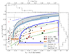 |
Fig. 1. He abundance (in number fraction in the lower x-axis, and in mass fraction in the upper one) against N abundances, for a sample of 180 Galactic O-type stars with v sin i ≤ 150 km s−1. Circles and crosses indicate LS and SB1 stars, respectively, while identified runaway stars are highlighted by red symbols. Typical uncertainties in He and N abundances are marked with a gray error bar in the upper left corner. HD 226868 (optical counterpart of Cyg X-1) is surrounded by a green circle. Blue and gray shadowed strips delimit the locations of solar-abundance single-star-evolution tracks associated with GENEC vini/vcrit = 0.2 and 0.4 model computations (Ekström et al. 2012, and priv. comm.) and MESA models following Keszthelyi et al. (2022), respectively. Baseline abundances for these models (from Ekström et al. 2012) are marked with a bluish-gray dot. The green shadowed strip outlines the location of single-star evolution tracks associated with GENEC vini/vcrit = 0.4 model computations for subsolar initial chemical composition (Eggenberger et al. 2021, see further discussion in Appendix B.3). Dotted lines correspond to two extreme cases of matter mixing at the stellar surface (see Appendix C). The blue-dotted line corresponds to mixing in which CNO-equilibrium is reached for any YHe value (considered initial values from Ekström et al. 2012). The green-dotted line corresponds to the mixing of pure He with material in CNO-equilibrium (considered initial values from Eggenberger et al. 2021, see the justification for this choice in the text). The shaded brown rectangle indicates the “cosmic abundance standard” obtained for early-B stars in the solar vicinity by Nieva & Przybilla (2012). The blue and orange (with dashed line) open contours surround the star samples with N and He abundance patterns not covered by the solar-abundance evolutionary models and not covered by the subsolar-abundance evolutionary models, respectively. Further details on the rationale for including the subsolar-abundances tracks can be found in Appendix B. Top and right: Histograms of He and N abundances, respectively. |
The shaded brown rectangle at the bottom left of the figure indicates the present-day cosmic (He and N) abundance standard suggested by Nieva & Przybilla (2012), resulting from the analysis of a sample of several tens of MS early B-type stars in the solar neighborhood (covering distances from the Sun up to ∼500 pc). This area of the diagram can be considered representative of the baseline abundances of our investigated sample of O-type stars, and it roughly coincides with the bluish-gray circle, which indicates the initial abundances assumed in the evolutionary models for solar metallicity.
Histograms of He and N abundances are shown in the top and rightmost panels. Error bars in the histograms were computed following a Markov Chains Monte Carlo (MCMC) approach, considering the individual uncertainties associated with the He and N abundance estimates. These uncertainties range within 20−30% in the case of He, and are typically on the order of ∼0.15 dex for the N abundances (see the gray cross in the upper left corner of the main panel, and further notes in Appendix B.1).
Despite the significant fraction of SSEM-outliers, the majority of the analyzed stars (∼75% of the sample) have normal-to-low He abundances (YHe < 0.12), and those objects exhibiting low values (20% of the sample with YHe < 0.09, which remains consistent with normal values considering typical uncertainties) will be further discussed in a forthcoming study. Nitrogen, on the other hand, appears to be approximately normally distributed, around ϵN ∼ 7.9 dex, with only a few extremely N-enriched objects.
4. Discussion
Single-star evolution models fail to explain the outliers found on the N-He plane (He enriched but N unenriched stars). Observational biases, lower initial abundances due to the present-day Galactic abundance gradient, or other unconsidered evolutionary pathways are also unlikely explanations (see Appendix B for a detailed discussion). Consequently, post-binary interaction presents itself as the most compelling origin for these objects.
4.1. Evolutionary model predictions
In single stars, internal mixing and wind stripping can make nuclear-processed material appear at the stellar surface. CNO equilibrium is achieved in the convective core near the beginning of MS evolution, before a significant mean-molecular-weight gradient develops at the core–envelope interface and before significant He-enrichment in the core. Helium, on the other hand, is synthesized in the core only on the nuclear timescale, and its mixture into the envelope is hindered by the corresponding mean-molecular-weight gradient. Also, mass loss uncovers the layers with the least He enrichment first, which are nevertheless still very N-enriched. This is why N-enhancement approximately precedes He-enhancement in single stars (self-enrichment).
For mass gainers in massive binary systems, the situation is different. During the mass transfer, at first, matter that is not greatly enriched, or is even pristine, is moved to the mass gainer. Towards the end, almost pure He is transferred, including N at its CNO-equilibrium value. The mixing of this matter with the envelope of a sufficiently massive gainer with an unmixed atmosphere – mainly composed of pristine gas – naturally leads to significant surface He enrichment with only modest N enhancement. This is shown by the comprehensive, detailed binary evolution models of Jin et al. (2024, and in prep., see also Appendix C).
As further described in Appendix C, binary interaction products can cover a much broader range in the YHe–ϵN plane compared to SSEM with the same initial composition. This is illustrated in Fig. 1 by the two dotted lines representing two extreme cases in which mixing of processed material reaching the stellar surface can occur. The upper limit (in blue) corresponds to the case in which CNO equilibrium is reached for any YHe value, with a CNO baseline consistent with solar values (second column of Table B.1). The lower boundary (in green) considers the mixing between the gas with the initial chemical composition and the pure He matter in CNO equilibrium, where a subsolar CNO baseline is assumed (third column of Table B.1). The latter was chosen to be consistent with stars with the lowest N abundance in our sample and to account for the possibility that some of the stars in our sample were born in regions with a subsolar composition (see Appendix B.3). Remarkably, most of the SSEM-outliers lie, within uncertainties, within the region limited by the two dotted lines. The only two targets that clearly remain below the green dotted line have been identified as SB1, where the dilution by contamination from the unseen companion could have affected the nitrogen determination.
In summary, stars identified as SSEM-outliers are not likely to have evolved in isolation, but are more likely to have been gainers in a binary system following a Roche-lobe overflow (RLOF) mass-transfer event.
4.2. Spectroscopic binaries and runaways
The binary origin of these systems is expected to result in two distinct dynamical outcomes following the mass-transfer event (see Fig. 4 and associated text in Marchant & Bodensteiner 2024). First, when the primary star completes its nuclear burning, it may undergo a supernova explosion, potentially disrupting the system and creating a runaway star if the kick’s direction and momentum are favorable (Blaauw 1961; van den Heuvel 1981, and reference therein). Given the short post-mass-transfer lifetime of the primary (as it has already left the MS) and a comparable rate of dynamical ejections associated with the star formation process for any type of single or multiple system (Poveda et al. 1967), this suggests a higher fraction of runaways among the SSEM-outliers.
Alternatively, if the system remains bound, the primary star is expected to lose its hydrogen envelope before the supernova explosion, becoming an optically faint stripped star (e.g., Paczyński 1967; Götberg et al. 2017; Yoon et al. 2017). As a result, the system would appear as an SB1, with either a compact object (e.g., Langer et al. 2020) or a stripped star (e.g., Paczyński 1967; Pols et al. 1991; Irrgang et al. 2020) as the companion, depending on whether or not a supernova has occurred. In this case, obtaining a rough estimation of the expected relative incidence of SB1 systems among the SSEM-outliers when compared to the population of pre-interaction binary system with a dimmer, low-mass companion is not straightforward.
Our observations show that 38 ± 6% of the SSEM-outliers are runaways, compared to 26 ± 3% in the rest of the sample, supporting our hypothesis. Notably, we also find a higher incidence of SB1 systems among the SSEM-outliers; 45 ± 7%, compared to 35 ± 4% in the rest of the sample. Further investigation into the companions of all detected SB1 systems in both subsamples could provide crucial insights to strengthen the likely post-binary interaction origin of the sample characterized by high He and unexpectedly low N surface abundances.
4.3. A representative case: Cyg X-1
Among the SSEM-outliers, we find the well-known high-mass X-ray binary HD 226868 (optical counterpart of Cyg X-1). It presents significant He enrichment (YHe = 0.18 ± 0.05) but a clear deficiency in N (8.08 ± 0.15 dex) compared to the SSEM predictions (ϵN ∼ 8.75 dex; see Fig. 1). This system hosts a black hole (BH) in a 5.6 day orbit, indicating that the visible component (an O9.7 Iab star) likely received mass at some point in its evolution from the initially more massive component (i.e., the progenitor of the BH). This would be in line with the binary-evolution scenario we are proposing.
This information has clear implications for the evolutionary scenario previously assumed for the formation of this system (Miller-Jones et al. 2021; Neijssel et al. 2021), pointing to an important mass-transfer phase of He-enriched material from the BH progenitor.
An abundance study of other known post-interaction candidates (e.g., Algols, Be stars, etc.; see Sen et al. 2022; Dufton et al. 2024) could help us to confirm our hypothesis. Nonetheless, the abundance determination in these types of sources remains challenging.
5. Final remarks
In this Letter, we present reliable N and He surface abundances for a subset of 180 O-stars with v sin i ≤ 150 km s−1 and well-defined stellar parameters. Within this sample, we find a subpopulation (∼20% of the total sample and ∼80% of helium-enriched stars) of interesting objects with a surface enrichment pattern in He and N. This group is unexplainable within the framework of single-star evolutionary models and cannot be associated with any observational or analytical biases (see further notes in Appendix B).
To explain this subset, we propose that its members are products of mass transfer in binary systems. Recent binary-evolution simulations support this hypothesis by qualitatively reproducing our results (see Appendix C), and can naturally explain the moderate N enrichment in strongly He-enhanced O stars. The higher prevalence of possible post-interaction outcomes (SB1 and runaways) among this subgroup supports this hypothesis. As a consequence of the proposed evolutionary scenario for these targets, the companions of the SB1 systems among them are promising candidates for stripped stars or black holes.
This study offers a critical observational reference for constraining key parameters of mass-transfer physics in close binary systems, particularly mass-transfer efficiency. Continued theoretical and observational efforts are crucial to deepen our understanding of massive-star evolution, be it in single or multiple star systems.
Non-rotating models do not produce remarkable surface enrichment during core hydrogen burning.
For simplicity, in both considered cases we assume that all the CNO isotopes convert into 14N.
Acknowledgments
We thank our anonymous referee for a set of useful comments and suggestions. This research acknowledges the support from the State Research Agency (AEI) of the Spanish Ministry of Science and Innovation and Universities (MCIU) and the European Regional Development Fund (FEDER) under grant PID2021-122397NB-C21. This publication made use of the IAC HTCondor facility (http://research.cs.wisc.edu/htcondor/), partly financed by the Ministry of Economy and Competitiveness with FEDER funds, code IACA13-3E-2493. C.M.S. acknowledges the workshop “Writing and Communicating your Science”, organised by the Severo Ochoa Training Programme of the IAA-CSIC and imparted by Henri Boffin (ESO) and Johan Knapen (IAC) on 4–8 November 2024. He also acknowledges Mar Carretero-Castrillo and Michelangelo Pantaleoni for kindly sharing their results on the runaway status of O Galactic stars for the statistical characterization of the sample. H.J. received financial support for this research from the International Max Planck Research School (IMPRS) for Astronomy and Astrophysics at the Universities of Bonn and Cologne. The authors gratefully acknowledge the granted access to the Bonna cluster hosted by the University of Bonn. Z.K. acknowledges support from JSPS Kakenhi Grant-in-Aid for Scientific Research (23K19071), the Overseas Visit Program for Young Researchers from the National Astronomical Observatory of Japan and the Early-Career Visitor Program from the Instituto de Astrofísica de Canarias. Numerical computations in part were carried out on the PC cluster at the Center for Computational Astrophysics, National Astronomical Observatory of Japan. J.P. acknowledges support from the Fundación Occident and the Instituto de Astrofísica de Canarias under the Visiting Researcher Programme 2022–2024 agreed between both institutions.
References
- Abdul-Masih, M. 2023, A&A, 669, L11 [NASA ADS] [CrossRef] [EDP Sciences] [Google Scholar]
- Aerts, C., Molenberghs, G., Kenward, M. G., & Neiner, C. 2014, ApJ, 781, 88 [Google Scholar]
- Aldoretta, E. J., Caballero-Nieves, S. M., Gies, D. R., et al. 2015, AJ, 149, 26 [Google Scholar]
- Arellano-Córdova, K. Z., Esteban, C., García-Rojas, J., & Méndez-Delgado, J. E. 2020, MNRAS, 496, 1051 [Google Scholar]
- Arellano-Córdova, K. Z., Esteban, C., García-Rojas, J., & Méndez-Delgado, J. E. 2021, MNRAS, 502, 225 [CrossRef] [Google Scholar]
- Asplund, M., Amarsi, A. M., & Grevesse, N. 2021, A&A, 653, A141 [NASA ADS] [CrossRef] [EDP Sciences] [Google Scholar]
- Bailer-Jones, C. A. L., Rybizki, J., Fouesneau, M., Demleitner, M., & Andrae, R. 2021, AJ, 161, 147 [Google Scholar]
- Barbá, R. H., Gamen, R., Arias, J. I., & Morrell, N. I. 2017, in The Lives and Death-Throes of Massive Stars, eds. J. J. Eldridge, J. C. Bray, L. A. S. McClelland, & L. Xiao, 329, 89 [Google Scholar]
- Blaauw, A. 1961, Bull. Astron. Inst. Netherlands, 15, 265 [NASA ADS] [Google Scholar]
- Bouret, J. C., Lanz, T., Martins, F., et al. 2013, A&A, 555, A1 [NASA ADS] [CrossRef] [EDP Sciences] [Google Scholar]
- Bouret, J. C., Martins, F., Hillier, D. J., et al. 2021, A&A, 647, A134 [NASA ADS] [CrossRef] [EDP Sciences] [Google Scholar]
- Brott, I., de Mink, S. E., Cantiello, M., et al. 2011, A&A, 530, A115 [NASA ADS] [CrossRef] [EDP Sciences] [Google Scholar]
- Cantiello, M., & Langer, N. 2010, A&A, 521, A9 [NASA ADS] [CrossRef] [EDP Sciences] [Google Scholar]
- Carneiro, L. P., Puls, J., Hoffmann, T. L., Holgado, G., & Simón-Díaz, S. 2019, A&A, 623, A3 [NASA ADS] [CrossRef] [EDP Sciences] [Google Scholar]
- Carretero-Castrillo, M., Ribó, M., & Paredes, J. M. 2023, A&A, 679, A109 [NASA ADS] [CrossRef] [EDP Sciences] [Google Scholar]
- de Mink, S. E., Pols, O. R., & Hilditch, R. W. 2007, A&A, 467, 1181 [NASA ADS] [CrossRef] [EDP Sciences] [Google Scholar]
- Dufton, P. L., Langer, N., Lennon, D. J., et al. 2024, MNRAS, 527, 5155 [Google Scholar]
- Eggenberger, P., Ekström, S., Georgy, C., et al. 2021, A&A, 652, A137 [NASA ADS] [CrossRef] [EDP Sciences] [Google Scholar]
- Ekström, S., Georgy, C., Eggenberger, P., et al. 2012, A&A, 537, A146 [Google Scholar]
- Evans, C. J., Smartt, S. J., Lee, J. K., et al. 2005, A&A, 437, 467 [NASA ADS] [CrossRef] [EDP Sciences] [Google Scholar]
- Evans, C. J., Taylor, W. D., Hénault-Brunet, V., et al. 2011, A&A, 530, A108 [NASA ADS] [CrossRef] [EDP Sciences] [Google Scholar]
- Frémat, Y., Zorec, J., Hubert, A. M., & Floquet, M. 2005, A&A, 440, 305 [NASA ADS] [CrossRef] [EDP Sciences] [Google Scholar]
- Götberg, Y., de Mink, S. E., & Groh, J. H. 2017, A&A, 608, A11 [NASA ADS] [CrossRef] [EDP Sciences] [Google Scholar]
- Grin, N. J., Ramírez-Agudelo, O. H., de Koter, A., et al. 2017, A&A, 600, A82 [NASA ADS] [CrossRef] [EDP Sciences] [Google Scholar]
- Herrero, A., Kudritzki, R. P., Vilchez, J. M., et al. 1992, A&A, 261, 209 [NASA ADS] [Google Scholar]
- Holgado, G., Simón-Díaz, S., Barbá, R. H., et al. 2018, A&A, 613, A65 [NASA ADS] [CrossRef] [EDP Sciences] [Google Scholar]
- Holgado, G., Simón-Díaz, S., Haemmerlé, L., et al. 2020, A&A, 638, A157 [NASA ADS] [CrossRef] [EDP Sciences] [Google Scholar]
- Holgado, G., Simón-Díaz, S., Herrero, A., & Barbá, R. H. 2022, A&A, 665, A150 [NASA ADS] [CrossRef] [EDP Sciences] [Google Scholar]
- Howarth, I. D., & Smith, K. C. 2001, MNRAS, 327, 353 [NASA ADS] [CrossRef] [Google Scholar]
- Hunter, I., Brott, I., Lennon, D. J., et al. 2008, ApJ, 676, L29 [NASA ADS] [CrossRef] [Google Scholar]
- Hunter, I., Brott, I., Langer, N., et al. 2009, A&A, 496, 841 [NASA ADS] [CrossRef] [EDP Sciences] [Google Scholar]
- Irrgang, A., Geier, S., Kreuzer, S., Pelisoli, I., & Heber, U. 2020, A&A, 633, L5 [NASA ADS] [CrossRef] [EDP Sciences] [Google Scholar]
- Jin, H., Langer, N., Lennon, D. J., & Proffitt, C. R. 2024, A&A, 690, A135 [NASA ADS] [CrossRef] [EDP Sciences] [Google Scholar]
- Keszthelyi, Z., Meynet, G., Georgy, C., et al. 2019, MNRAS, 485, 5843 [NASA ADS] [CrossRef] [Google Scholar]
- Keszthelyi, Z., de Koter, A., Götberg, Y., et al. 2022, MNRAS, 517, 2028 [Google Scholar]
- Kippenhahn, R., Ruschenplatt, G., & Thomas, H. C. 1980, A&A, 91, 175 [Google Scholar]
- Langer, N. 2012, ARA&A, 50, 107 [CrossRef] [Google Scholar]
- Langer, N., & Kudritzki, R. P. 2014, A&A, 564, A52 [NASA ADS] [CrossRef] [EDP Sciences] [Google Scholar]
- Langer, N., Schürmann, C., Stoll, K., et al. 2020, A&A, 638, A39 [NASA ADS] [CrossRef] [EDP Sciences] [Google Scholar]
- Lester, J. B. 1973, ApJ, 185, 253 [NASA ADS] [CrossRef] [Google Scholar]
- Lyubimkov, L. S. 1996, Ap&SS, 243, 329 [NASA ADS] [CrossRef] [Google Scholar]
- Maeder, A., & Meynet, G. 2000, ARA&A, 38, 143 [Google Scholar]
- Maíz Apellániz, J., Sota, A., Morrell, N. I., et al. 2013, Massive Stars: From alpha to Omega, 198 [Google Scholar]
- Maíz Apellániz, J., Pantaleoni González, M., Barbá, R. H., et al. 2018, A&A, 616, A149 [NASA ADS] [CrossRef] [EDP Sciences] [Google Scholar]
- Maíz Apellániz, J., Trigueros Páez, E., Negueruela, I., et al. 2019, A&A, 626, A20 [NASA ADS] [CrossRef] [EDP Sciences] [Google Scholar]
- Maíz Apellániz, J., Trigueros Páez, E., Negueruela, I., et al. 2020, A&A, 639, C1 [NASA ADS] [CrossRef] [EDP Sciences] [Google Scholar]
- Marchant, P., & Bodensteiner, J. 2024, ARA&A, 62, 21 [NASA ADS] [CrossRef] [Google Scholar]
- Markova, N., Puls, J., & Langer, N. 2018, A&A, 613, A12 [NASA ADS] [CrossRef] [EDP Sciences] [Google Scholar]
- Martins, F., Hervé, A., Bouret, J. C., et al. 2015, A&A, 575, A34 [NASA ADS] [CrossRef] [EDP Sciences] [Google Scholar]
- Martins, F., Simón-Díaz, S., Barbá, R. H., Gamen, R. C., & Ekström, S. 2017, A&A, 599, A30 [NASA ADS] [CrossRef] [EDP Sciences] [Google Scholar]
- Martins, F., Bouret, J. C., Hillier, D. J., et al. 2024, A&A, 689, A31 [NASA ADS] [CrossRef] [EDP Sciences] [Google Scholar]
- Miller-Jones, J. C. A., Bahramian, A., Orosz, J. A., et al. 2021, Science, 371, 1046 [Google Scholar]
- Morel, T., Butler, K., Aerts, C., Neiner, C., & Briquet, M. 2006, A&A, 457, 651 [NASA ADS] [CrossRef] [EDP Sciences] [Google Scholar]
- Neijssel, C. J., Vinciguerra, S., Vigna-Gómez, A., et al. 2021, ApJ, 908, 118 [NASA ADS] [CrossRef] [Google Scholar]
- Nieva, M. F., & Przybilla, N. 2012, A&A, 539, A143 [NASA ADS] [CrossRef] [EDP Sciences] [Google Scholar]
- Paczyński, B. 1967, Acta Astron., 17, 355 [NASA ADS] [Google Scholar]
- Paxton, B., Marchant, P., Schwab, J., et al. 2015, ApJS, 220, 15 [Google Scholar]
- Pinsonneault, M. H., Kawaler, S. D., Sofia, S., & Demarque, P. 1989, ApJ, 338, 424 [Google Scholar]
- Pols, O. R., Cote, J., Waters, L. B. F. M., & Heise, J. 1991, A&A, 241, 419 [NASA ADS] [Google Scholar]
- Potter, A. T., Chitre, S. M., & Tout, C. A. 2012, MNRAS, 424, 2358 [NASA ADS] [CrossRef] [Google Scholar]
- Poveda, A., Ruiz, J., & Allen, C. 1967, Boletin de los Observatorios Tonantzintla y Tacubaya, 4, 86 [Google Scholar]
- Puls, J., Urbaneja, M. A., Venero, R., et al. 2005, A&A, 435, 669 [NASA ADS] [CrossRef] [EDP Sciences] [Google Scholar]
- Ramírez-Agudelo, O. H., Sana, H., de Mink, S. E., et al. 2015, A&A, 580, A92 [NASA ADS] [CrossRef] [EDP Sciences] [Google Scholar]
- Rivero González, J. G., Puls, J., & Najarro, F. 2011, A&A, 536, A58 [NASA ADS] [CrossRef] [EDP Sciences] [Google Scholar]
- Rivero González, J. G., Puls, J., Najarro, F., & Brott, I. 2012, A&A, 537, A79 [NASA ADS] [CrossRef] [EDP Sciences] [Google Scholar]
- Sana, H., de Mink, S. E., de Koter, A., et al. 2012, Science, 337, 444 [Google Scholar]
- Sana, H., Le Bouquin, J. B., Lacour, S., et al. 2014, ApJS, 215, 15 [Google Scholar]
- Santolaya-Rey, A. E., Puls, J., & Herrero, A. 1997, A&A, 323, 488 [NASA ADS] [Google Scholar]
- Schonberner, D., Herrero, A., Becker, S., et al. 1988, A&A, 197, 209 [NASA ADS] [Google Scholar]
- Schootemeijer, A., Götberg, Y., de Mink, S. E., Gies, D., & Zapartas, E. 2018, A&A, 615, A30 [NASA ADS] [CrossRef] [EDP Sciences] [Google Scholar]
- Schürmann, C., & Langer, N. 2024, A&A, 691, A174 [NASA ADS] [CrossRef] [EDP Sciences] [Google Scholar]
- Sen, K., Langer, N., Marchant, P., et al. 2022, A&A, 659, A98 [NASA ADS] [CrossRef] [EDP Sciences] [Google Scholar]
- Shenar, T., Bodensteiner, J., Sana, H., et al. 2024, A&A, 690, A289 [NASA ADS] [CrossRef] [EDP Sciences] [Google Scholar]
- Simón-Díaz, S., & Herrero, A. 2014, A&A, 562, A135 [NASA ADS] [CrossRef] [EDP Sciences] [Google Scholar]
- Simón-Díaz, S., Castro, N., Herrero, A., et al. 2011, J. Phys. Conf. Ser., 328, 012021 [Google Scholar]
- Simón-Díaz, S., Pérez Prieto, J. A., Holgado, G., de Burgos, A., & Iacob Team 2020, XIV.0 Scientific Meeting (virtual) of the Spanish Astronomical Society, 187 [Google Scholar]
- Simón-Díaz, S., Britavskiy, N., Castro, N., Holgado, G., & de Burgos, A. 2024, ArXiv e-prints [arXiv:2405.11209] [Google Scholar]
- Takahashi, K., & Langer, N. 2021, A&A, 646, A19 [NASA ADS] [CrossRef] [EDP Sciences] [Google Scholar]
- van den Heuvel, E. P. J. 1981, Space Sci. Rev., 30, 623 [NASA ADS] [CrossRef] [Google Scholar]
- Villaseñor, J. I., Taylor, W. D., Evans, C. J., et al. 2021, MNRAS, 507, 5348 [CrossRef] [Google Scholar]
- Vinciguerra, S., Neijssel, C. J., Vigna-Gómez, A., et al. 2020, MNRAS, 498, 4705 [NASA ADS] [CrossRef] [Google Scholar]
- von Zeipel, H. 1924, MNRAS, 84, 665 [NASA ADS] [CrossRef] [Google Scholar]
- Wellstein, S., & Langer, N. 1999, A&A, 350, 148 [NASA ADS] [Google Scholar]
- Yoon, S.-C., Dessart, L., & Clocchiatti, A. 2017, ApJ, 840, 10 [NASA ADS] [CrossRef] [Google Scholar]
- Zahn, J. P. 1992, A&A, 265, 115 [NASA ADS] [Google Scholar]
Appendix A: Stellar evolution models
In this Appendix, we outline some of the main characteristics of the two grids of solar metallicity, single-star evolutionary models used to compare with our observational data. Additionally, Table B.1 displays the initial set of C, N, and O abundances considered by each of the models.
Ekström et al. models
Ekström et al. (2012) used the Geneva stellar evolution code, GENEC, to compute the model grids utilized in the current Letter. Convection is assumed as an instantaneous mixing process and αMLT = 1.6 is adopted. A step overshooting with αov = 0.1 is used, leading to a radial extension of the nominal convective core size by 10 percent of the local pressure scale height. The initial abundances of hydrogen, helium, and metals are adopted as X = 0.720, Y = 0.266, and Z = 0.014, respectively. Initial abundances from C, N, and O can be found in Table B.1. Rotational mixing is considered via diffusion coefficients that account for effective diffusivity (combining meridional circulation and horizontal diffusion) and shear diffusion. Angular momentum transport follows an advecto-diffusive scheme, in which meridional currents can increase the radial differential rotation and thus shears can become the dominant term for chemical mixing. Rotation is assumed with v/vcrit = 0, 0.2, 0.4. The critical velocity is defined as the velocity at which the gravitational acceleration is exactly counterbalanced by the centrifugal force;  , where Rpb is the polar radius at the critical limit. The mass of the grid extends from 0.8 to 120 M⊙.
Keszthelyi et al. models
Keszthelyi et al. (2022) used the community-driven, open-source Modules for Experiments in Stellar Astrophyscs, MESA, software (e.g., Paxton et al. 2015). Convective mixing is considered a diffusive process with an efficiency of αMLT = 1.8, and exponential overshooting is adopted with fov = 0.025 and f0 = 0.005, which would roughly correspond to αov = 0.2. For their solar metallicity models, the initial abundances of X, Y, Z are the same as in the Ekström et al. (2012) grid. The initial C, N, and O abundances are obtained from the determination of Nieva & Przybilla (2012) and thus the values are slightly different used by Ekström et al. (2012) (see first and third column in Table B.1).
Due to the uncertain nature of chemical mixing, two schemes are implemented. "Mix1" follows the typical MESA approach, utilizing the prescriptions developed by Pinsonneault et al. (1989), and using scaling factors to mitigate the otherwise too efficient mixing (compared to angular momentum transport). The "Mix2" scheme is the implementation of the Zahn (1992) equations, similar to the study of Ekström et al. (2012). Angular momentum transport follows a diffusive approximation. In this case, the Eddington-Sweet term is the dominant one for both angular momentum transport and chemical mixing. For this reason, the Mix2 models are still considerably different than those of Ekström et al. (2012), since the underlying rotation profiles are distinct. In fact, the Mix2 models lead to quasi-chemically homogeneous evolution, which is the most efficient form of mixing in a star. Rotation is assumed with an initial value of Ω/Ωcrit = 0.5, corresponding to ≈350 km s−1. The initial mass range of the grid is from 3 to 60 M⊙. For this study, it was beneficial to extend the parameter space of this grid, for which we computed new models. These include initial masses of 80, 90, and 100 M⊙, and initial rotation values of Ω/Ωcrit = 0.1, 0.2, 0.3, 0.4 were additionally considered for the initial mass range of 20 - 100 M⊙.
Appendix B: Potential single-star evolution origin of the SSEM-outliers
In this Appendix, we summarize the main outcomes from our study exploring a potential single-star evolutionary origin of the SSEM-outliers.
Potential errors and biases in the spectroscopic analysis
Initially, we examined whether potential analysis errors could affect the accuracy of our He and N abundance measurements. In particular, we took a conservative approach when addressing formal uncertainties, considering the impact of EW measurements, the scatter from individual lines, stellar parameters, and microturbulence. We also performed a MCMC analysis to identify the SSEM-outliers based on their distribution in the YHe-ϵN abundance diagram. Furthermore, we carefully defined the boundaries of the blue open contour around the SSEM-outliers to ensure that, even with uncertainties, these stars could not be explained by single-star evolution models.
It is also unlikely that a bias in the N abundance determination could explain the predominantly low values observed among the SSEM-outliers. Any inherent observational bias would likely skew measurements toward higher ϵN values, as lower abundances result in fainter spectral lines that are harder to measure, potentially leading to the exclusion of such stars. In contrast, He exhibits stronger lines, making a high-abundance bias negligible. However, dilution effects from external contamination in the continuum could slightly underestimate He abundance.
Gravity darkening effects
In SSEM, rotational mixing is expected to be the primary driver of surface contamination by CNO-cycle products. For O-type stars, He enrichment (i.e., YHe ≳ 0.12) is expected to be detectable only in stars with initial masses above ∼ 30 M⊙ and equatorial rotational velocities at birth exceeding 300 km s−1 (e.g., Ekström et al. 2012, see also Fig. B.2). While significant braking of the stellar surface is predicted to occur during the first half of the MS evolution under certain conditions (see, e.g., Ekström et al. 2012; Keszthelyi et al. 2022; Holgado et al. 2022), not all SSEM scenarios result in this outcome (e.g., Brott et al. 2011). Consequently, some stars in our sample may still be fast rotators with relatively low inclination angles (as we are limited to v sin i ≤ 150 km s−1).
In this context, as noted by Frémat et al. (2005) and Abdul-Masih (2023), neglecting the 3D deformations caused by rapid rotation, including the effects of gravity darkening (von Zeipel 1924), can significantly impact stellar parameters and abundance determinations. Abdul-Masih (2023) highlights a temperature-dependent discrepancy in helium abundance that could notably deviate from the actual value. Furthermore, potentially similar effects in nitrogen warrant an investigation. However, the probability that all SSEM-outliers are fast rotators observed at near pole-on orientations is negligible (e.g., Holgado et al. 2022).
Impact of baseline abundances
We investigated the influence of the baseline abundances in the interpretation of our results. In particular, we studied the possibility that some of the SSEM-outliers correspond to stars with an initial CNO composition lower than solar.
Our stars reach distances up to ∼ 4 kpc from the Sun (Fig. B.1). However, this distribution is not homogeneous. Most stars are located within approximately 3 kpc, with this distance decreasing to around 2 kpc in the direction of the Galactic anticenter. Overall, the initial abundances in our sample are affected by the Galactic chemical abundance gradient. Arellano-Córdova et al. (2020, 2021) investigated the present-day gradient of the Galactic disc as delineated by H II regions. Together with the Cosmic Abundance Standard (CAS) from Nieva & Przybilla (2012), it gives us a rough estimate of the minimum expected initial C, N, and O abundances for our sample of ∼8.1, 7.6, and 8.6 dex, respectively. This could explain the existence of stars with N abundances below CAS in Fig. 1 (shaded brown rectangle).
For the comparative purpose of this section, we found the SSEM of Eggenberger et al. (2021) to be the most appropriate. Those models were computed with the GENEC code for a metallicity Z ∼ 0.45 Z⊙ (i.e., a value typically considered for the LMC). For the initial abundances of elements heavier than He, they scaled the value from Ekström et al. (2012) with metallicity (Table B.1). The resulting initial CNO composition is below the minimum expected abundances inferred from the gradient of the Milky Way disc. Moreover, it reaches the lowest end of our N abundance distribution in Fig. 1.
Carbon, nitrogen, and oxygen initial abundances of the models considered.
As the main result of this exercise, we found that when we consider such an extreme case of lower baseline abundances – inappropriate for our sample –, we could account for some of our problematic sources. Still, even in this extreme scenario, about 10% of the analyzed stars would retain their status as SSEM-outliers (see stars surrounded by the orange contour in Fig 1). Moreover, a similar argument based on the Galactic gradient could lead to more sources closer to the Galactic Center appearing as SSEM-outliers.
SSEM-outliers in the spectroscopic HR diagram
Figure B.2 shows the location of the 180 Galactic O-type stars from our sample in the spectroscopic HR diagram (sHRD, introduced by Langer & Kudritzki 2014). SSEM-outliers are marked with star symbols. Among these, those explainable by SSEM with subsolar baseline abundances are shown in dark blue, while the remaining outliers, even in this extreme case, are highlighted in orange. The latter group clusters in the cooler region of the diagram (30 ≲ Teff/kK ≲ 35), whereas the former spans a wider temperature range (32 ≲ Teff/kK ≲ 43).
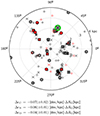 |
Fig. B.1. Top: Spatial distribution of our sample of O-type stars in the Galactic plane, with the Sun (⊙) at the center. Same marker code as in Fig. 1. Bottom: Values of the Galactic present-day abundance gradient of C, N, O as a function of galactocentric distance (RG), from Arellano-Córdova et al. (2020, 2021). Distances from Bailer-Jones et al. (2021) |
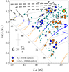 |
Fig. B.2. Spectroscopic HRD of the 180 Galactic O-type stars studied, with SSEM-outliers marked by star symbols. Orange stars indicate those that remain outliers even when assuming Eggenberger et al. (2021) models (subsolar baseline abundances). HD 226868, the optical counterpart of Cyg X-1, is circled in green. Non-rotating and vini/vcrit = 0.4 evolutionary tracks from Ekström et al. (2012) are shown for reference (see text for details). Typical uncertainties in Teff and log ℒ are represented by a gray cross. |
The figure also includes the SSEM tracks from Ekström et al. (2012), both without rotation (solid lines) and with an initial rotational velocity of 40% of the critical value (dashed lines). For the rotating models2, we divide the tracks into three regions based on the surface N abundance, following the behavior of evolutionary models in Fig. 1. The regions are marked by an orange-dotted line, a blue dashed-dotted line, and a gray dashed line, representing ϵN ≤ 8.25 dex, 8.25 < ϵN ≤ 8.6 dex, and ϵN > 8.6 dex, respectively. The 8.25 value represents the maximum N enrichment in subsolar abundances models, while 8.6 corresponds to the solar-abundance models. In addition, we highlight (by thick lines) the regions of the tracks where YHe ≥ 0.12. Remarkably, this value is not reached during the MS for initial masses below ∼30 M⊙, and is only reached after the stars exhibit CNO-equilibrium (ϵN > 8.6 dex).
The overall agreement between observational data for the SSEM-outliers and predictions from the rotating models is very weak. A significant portion of the sample (to repeat in different units: particularly stars with log(ℒ/ℒ⊙) ≲ 3.8 dex, corresponding to the afore-mentioned tracks below ∼30 M⊙) is not expected to reach YHe > 0.12 during the MS. While higher-mass stars are predicted to show some helium enrichment, this is never consistent with the low N abundances observed in the objects marked with star symbols (see Table D.1).
Finally, efficient rotational mixing should lead to increased N at the surface when stars evolve away from the ZAMS. Consequently, those objects marked with orange symbols (i.e., SSEM-outliers with lower N abundances) would be expected to lie closer to the ZAMS than the blue-marked SSEM-outliers. Their distribution should roughly overlap with the region of the rotating tracks highlighted in orange. However, Fig. B.2 shows the opposite trend, complicating the interpretation of these SSEM-outliers as products of single-star evolution.
Appendix C: Comparing models of mass gainers and of single stars
Figure C.1 compares the surface He and N abundance predictions from detailed models of single stars and mass gainers in binary systems. Both sets of models were computed with MESA under similar physical assumptions (Jin et al. 2024, and in prep.). Initial abundances in all models are based on the protosolar values from Asplund et al. (2021), which differ from those used in the SSEM by Ekström et al. (2012) and Keszthelyi et al. (2022) (Table B.1).
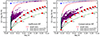 |
Fig. C.1. Location of single and binary evolutionary models from Jin et al. (2024, and in prep.) in the N vs. He diagram. The extended pink line covers the evolutionary tracks of the SSEM described in Appendix C. Mass gainers predictions are depicted immediately before mass transfer (MT; cyan dots), and after mass transfer at a time when thermal equilibrium is restored (magenta dots). Left and right panels depict MESA calculations assuming an inefficient or conservative mass transfer, respectively. The dotted-blue line shows abundance ratios under the assumption of complete CNO-equilibrium at any given He abundance. The dotted-green line has the same meaning but assuming a mixture between matter with the initial chemical composition and matter consisting of pure He and the CNO-equilibrium value of N (with a mass fraction indicated by along the red dots). Both dotted lines frame the allowed space for evolutionary models. The dotted-black line refers to a mixture of matter with the initial abundances with matter with a He mass fraction of Y = 0.63, corresponding to the average in the He-enriched part of the donor envelopes, and the CNO-equilibrium value of N. |
The single star models cover an initial mass range of Mi = 10 – 100 M⊙. Models with Mi = 10 – 40 M⊙ are taken from Jin et al. (2024), while those for higher masses have been coherently computed afterwards. In all these models, initial rotation was set to v/vcrit = 0.4
Mass gainer predictions are taken from a comprehensive grid of detailed binary evolution models consisting of ∼38 000 initial configurations. These cover primary star masses in the range 5 – 100 M⊙, mass ratios of 0.1 – 0.95, and orbital periods ranging from that resulting in Roche-lobe filling at zero-age MS (ZAMS) to non-interaction. In all cases, the initial rotation rate was set to vi/vcrit = 0.2.
In order to match the evolutionary masses of the observed stars (Fig. B.2), the two panels in Fig. C.1 only depict predictions for mass gainers with M > 15 M⊙. Each mass gainer is represented by a single point in the N vs. He diagrams. In particular, the considered abundances correspond to the moment when the mass gainer has thermally relaxed after the mass transfer event and thermohaline mixing of the enriched matter has taken place. Thermohaline mixing is treated as a diffusive process in MESA, with a parameter αth determining the speed of mixing. We adopt αth = 1 (Kippenhahn et al. 1980). Thermohaline mixing occurs on the thermal timescale (Cantiello & Langer 2010). Consequently, the envelope of the mass gainer will achieve full mixing on a short timescale compared to the post-interaction MS lifetime. After this phase, the surface abundances change minimally.
In the original calculations by Jin et al. (in prep.), the amount of accreted mass was limited by the rotation of the mass gainer. When spin-down due to tides is inefficient, mass transfer is highly non-conservative, and mass gainers end up accreting only a few percent of the transferred mass (Langer 2012). However, the mass transfer physics and its efficiency are not well-constrained, and there are several pieces of evidence supporting a higher mass transfer efficiency (e.g., Wellstein & Langer 1999; de Mink et al. 2007; Schootemeijer et al. 2018; Vinciguerra et al. 2020). Thus, in addition to exploring the original mass gainer models (left panel of Fig. C.1), we recompute the chemical envelope structure of the mass gainers assuming fully conservative mass transfer (right panel).
For the conservative mass transfer case, we estimated the composition of the mass gainer by assuming that all the transferred mass is accreted onto the mass gainer and, subsequently, the polluted envelope is fully mixed with the original material. The accreted matter is mixed down partly into the H/He composition gradient such that the mean molecular weight of the fully mixed matter in the envelope is the same as that of the layer in the H/He composition gradient. This is expected when thermohaline mixing has fully taken place. Noteworthy, we consider only binary models which are expected to survive the conservative mass transfer. To this aim, we compare the thermal timescale and the mass gain timescale of the mass gainer following Schürmann & Langer (2024). In particular, we assume  when considering their eq. 5, where
  is the change of the mass per unit time of the mass gainer,
  is the mass transfer rate from the donor, Menv, 1 and τKH, 1 are the envelope mass and the thermal timescale of the donor. As for the inefficient mass transfer case, we only depict in Fig. C.1 (right figure) those mass gainers with M > 15 M⊙.
Mass gainers will become fast rotators and rotational mixing will be enhanced. However, the mean molecular weight gradient already established above the core will likely prevent the inner nuclear-processed matter (He-rich, N-rich) from being transported to the surface (see discussion in Sect. 6.2 of Dufton et al. 2024). Moreover, as we consider the full mixing of the accreted matter, we do not expect rotational mixing to further affect surface abundances. Only under the scenario of the mass gainer already fast rotating before the mass accretion, the mass gainers would show surface N-enhancement closer to the CNO equilibrium value. However, this is unlikely when assuming that the initial rotation rates of MS binary components are following the same distribution as those of single stars, as Ramírez-Agudelo et al. (2015) found for O star binaries in the LMC.
As shown in Fig. C.1, for a given He enrichment, the mass gainer models display a much weaker N enrichment than the single star models. In the latter, mixing processes can bring N much easier to the surface than He, a fact which is irrelevant for the mass gainers. While conservative mass transfer can lead to higher He enrichments than inefficient mass transfer, the offset of the mass gainer models from the single-star models is evident in both cases.
For reference purposes, we indicate in both panels of Fig. C.1 the extreme cases in between which any stellar evolution model must lie3. The blue-dotted line assumes CNO-equilibrium is reached for any given He abundance

while the green-dotted line is obtained by mixing pure He matter, which is in CNO equilibrium,

where He/H and N/H represent number fractions, while Yi, XN, i, and XCNO, i indicate initial mass fractions of He, N, and C+N+O, respectively. These reference limits have been taken into account for the discussion presented in Sect. 4.1 (see also Fig. 1).
Appendix D: Stellar parameters for SSEM-outliers
Table D.1 summarizes observational information of interest about the 36 SSEM-outliers surrounded by a blue contour in Fig. 1 and highlighted with larger, bold symbols.
Stellar parameters of the SSEM-outliers.
All Tables
All Figures
|
Fig. 1. He abundance (in number fraction in the lower x-axis, and in mass fraction in the upper one) against N abundances, for a sample of 180 Galactic O-type stars with v sin i ≤ 150 km s−1. Circles and crosses indicate LS and SB1 stars, respectively, while identified runaway stars are highlighted by red symbols. Typical uncertainties in He and N abundances are marked with a gray error bar in the upper left corner. HD 226868 (optical counterpart of Cyg X-1) is surrounded by a green circle. Blue and gray shadowed strips delimit the locations of solar-abundance single-star-evolution tracks associated with GENEC vini/vcrit = 0.2 and 0.4 model computations (Ekström et al. 2012, and priv. comm.) and MESA models following Keszthelyi et al. (2022), respectively. Baseline abundances for these models (from Ekström et al. 2012) are marked with a bluish-gray dot. The green shadowed strip outlines the location of single-star evolution tracks associated with GENEC vini/vcrit = 0.4 model computations for subsolar initial chemical composition (Eggenberger et al. 2021, see further discussion in Appendix B.3). Dotted lines correspond to two extreme cases of matter mixing at the stellar surface (see Appendix C). The blue-dotted line corresponds to mixing in which CNO-equilibrium is reached for any YHe value (considered initial values from Ekström et al. 2012). The green-dotted line corresponds to the mixing of pure He with material in CNO-equilibrium (considered initial values from Eggenberger et al. 2021, see the justification for this choice in the text). The shaded brown rectangle indicates the “cosmic abundance standard” obtained for early-B stars in the solar vicinity by Nieva & Przybilla (2012). The blue and orange (with dashed line) open contours surround the star samples with N and He abundance patterns not covered by the solar-abundance evolutionary models and not covered by the subsolar-abundance evolutionary models, respectively. Further details on the rationale for including the subsolar-abundances tracks can be found in Appendix B. Top and right: Histograms of He and N abundances, respectively. |
| In the text | |
|
Fig. B.1. Top: Spatial distribution of our sample of O-type stars in the Galactic plane, with the Sun (⊙) at the center. Same marker code as in Fig. 1. Bottom: Values of the Galactic present-day abundance gradient of C, N, O as a function of galactocentric distance (RG), from Arellano-Córdova et al. (2020, 2021). Distances from Bailer-Jones et al. (2021) |
| In the text | |
|
Fig. B.2. Spectroscopic HRD of the 180 Galactic O-type stars studied, with SSEM-outliers marked by star symbols. Orange stars indicate those that remain outliers even when assuming Eggenberger et al. (2021) models (subsolar baseline abundances). HD 226868, the optical counterpart of Cyg X-1, is circled in green. Non-rotating and vini/vcrit = 0.4 evolutionary tracks from Ekström et al. (2012) are shown for reference (see text for details). Typical uncertainties in Teff and log ℒ are represented by a gray cross. |
| In the text | |
|
Fig. C.1. Location of single and binary evolutionary models from Jin et al. (2024, and in prep.) in the N vs. He diagram. The extended pink line covers the evolutionary tracks of the SSEM described in Appendix C. Mass gainers predictions are depicted immediately before mass transfer (MT; cyan dots), and after mass transfer at a time when thermal equilibrium is restored (magenta dots). Left and right panels depict MESA calculations assuming an inefficient or conservative mass transfer, respectively. The dotted-blue line shows abundance ratios under the assumption of complete CNO-equilibrium at any given He abundance. The dotted-green line has the same meaning but assuming a mixture between matter with the initial chemical composition and matter consisting of pure He and the CNO-equilibrium value of N (with a mass fraction indicated by along the red dots). Both dotted lines frame the allowed space for evolutionary models. The dotted-black line refers to a mixture of matter with the initial abundances with matter with a He mass fraction of Y = 0.63, corresponding to the average in the He-enriched part of the donor envelopes, and the CNO-equilibrium value of N. |
| In the text | |
Current usage metrics show cumulative count of Article Views (full-text article views including HTML views, PDF and ePub downloads, according to the available data) and Abstracts Views on Vision4Press platform.
Data correspond to usage on the plateform after 2015. The current usage metrics is available 48-96 hours after online publication and is updated daily on week days.
Initial download of the metrics may take a while.