| Issue |
A&A
Volume 695, March 2025
|
|
|---|---|---|
| Article Number | A197 | |
| Number of page(s) | 18 | |
| Section | Stellar atmospheres | |
| DOI | https://doi.org/10.1051/0004-6361/202451366 | |
| Published online | 20 March 2025 | |
X-Shooting ULLYSES: Massive stars at low metallicity
X. Physical parameters and feedback of massive stars in the LMC N11 B star-forming region
1
Institut für Physik und Astronomie, Universität Potsdam,
Karl-Liebknecht-Str. 24/25,
14476
Potsdam, Germany
2
Zentrum für Astronomie der Universität Heidelberg, Astronomisches Rechen-Institut,
Mönchhofstr. 12–14,
69120
Heidelberg, Germany
3
Armagh Observatory and Planetarium,
College Hill
BT61 9DG,
Armagh, Northern Ireland,
UK
4
Department of Physics & Astronomy, University of Sheffield, Hicks Building,
Hounsfield Road,
Sheffield
S3 7RH, UK
5
Dpto. de Astrofísica, Universidad de La Laguna,
38205
La Laguna, Tenerife,
Spain
6
Instituto de Astrofísica de Canarias,
38200
La Laguna, Tenerife,
Spain
7
Penn State Scranton,
120 Ridge View Drive,
Dunmore,
PA
18512, USA
8
Astronomický ústav, Akademie věd České republiky,
Fričova 298,
251 65
Ondřejov, Czech Republic
9
Departamento de Ciencias, Facultad de Artes Liberales, Universidad Adolfo Ibáñez,
Viña del Mar
Chile
10
Instituto de Astrofísica, Facultad de Física, Pontificia Universidad Católica de Chile,
782-0436
Santiago, Chile
11
Instituto de Astrofísica de Andalucía,
Glorieta de la Astronomía s/n,
18008
Granada,
Spain
12
Faculty of Physics, University of Duisburg-Essen,
Lotharstraße 1,
47057
Duisburg, Germany
13
Space Telescope Science Institute,
3700 San Martin Drive,
Baltimore,
MD
21218, USA
14
Royal Observatory of Belgium,
Avenue Circulaire/Ringlaan 3,
1180
Brussels, Belgium
15
Centre for Extragalactic Astronomy, Department of Physics, Durham University,
South Road,
Durham
DH1 3LE, UK
16
Institute for Computational Cosmology, Department of Physics, University of Durham,
South Road,
Durham
DH1 3LE, UK
17
European Organisation for Astronomical Research in the Southern Hemisphere,
Alonso de Cordova 3107,
Vitacura, Santiago de Chile
Chile
18
The School of Physics and Astronomy, Tel Aviv University,
Tel Aviv
6997801, Israel
19
Carnegie Observatories, Las Campanas Observatory,
Casilla 601,
La Serena,
Chile
20
Department of Astrophysical Sciences, Princeton University,
4 Ivy Lane,
Princeton,
NJ
08544, USA
21
The Observatories of the Carnegie Institution for Science,
813 Santa Barbara Street,
Pasadena,
CA
91101, USA
22
Lennard-Jones Laboratories, Keele University,
ST5 5BG,
UK
23
Centro de Astrobiología, CSIC-INTA,
Carretera de Ajalvir km 4,
28850
Torrejón de Ardoz, Madrid,
Spain
24
Instituto de Astronomía, UNAM, Unidad Académica en Ensenada,
Km 103 Carr.
Tijuana–Ensenada, Ensenada,
BC 22860, Mexico
★ Corresponding author; This email address is being protected from spambots. You need JavaScript enabled to view it.
Received:
3
July
2024
Accepted:
21
November
2024
Abstract
Massive stars drive the ionization and mechanical feedback within young star-forming regions. The Large Magellanic Cloud (LMC) is an ideal galaxy for studying individual massive stars and quantifying their feedback contribution to the environment. We analyze eight exemplary targets in LMC N11 B from the Hubble UV Legacy Library of Young Stars as Essential Standards (ULLYSES) program using novel spectra from HST (COS and STIS) in the UV, and from VLT (X-shooter) in the optical. We model the spectra of early to late O-type stars using state-of-the-art PoWR atmosphere models. We determine the stellar and wind parameters (e.g., T⋆, log g, L⋆, Ṁ, and v∞) of the analyzed objects, chemical abundances (C, N, and O), ionizing and mechanical feedback (QH, QHeI, QHe II, and Lmec), and X-rays. We report ages of 2–4.5 Myr and masses of 30–60 M⊙ for the analyzed stars in N11 B, which are consistent with a scenario of sequential star formation. We note that the observed wind-momentum–luminosity relation is consistent with theoretical predictions. We detect nitrogen enrichment by up to a factor of seven in most of the stars. However, we do not find a correlation between nitrogen enrichment and projected rotational velocity. Finally, based on their spectral type, we estimate the total ionizing photons injected from the O-type stars in N11 B into its environment. We report log (Σ QH) = 50.5 ph s−1, log (Σ QHe I) = 49.6 ph s−1, and log (Σ QHe II)= 44.4 ph s−1, consistent with the total ionizing budget in N11.
Key words: stars: atmospheres / stars: fundamental parameters / stars: massive / stars: mass-loss / stars: winds, outflows / HII regions
© The Authors 2025
 Open Access article, published by EDP Sciences, under the terms of the Creative Commons Attribution License (https://creativecommons.org/licenses/by/4.0), which permits unrestricted use, distribution, and reproduction in any medium, provided the original work is properly cited.
This article is published in open access under the Subscribe to Open model. This email address is being protected from spambots. You need JavaScript enabled to view it. to support open access publication.
1 Introduction
Massive stars, defined as those with initial masses (Mi) on the main sequence of ≥8 M⊙, are key to understanding multiple astrophysical phenomena: from fundamental nucleosynthesis processes (e.g., CNO cycle and He-burning) to interstellar medium (ISM) feedback; such as the injection of mechanical energy, ionizing photons, and fresh elements from stars into their local environment. Thus, massive stars are expected to have a significant impact on the evolution of their host galaxies (see Massey 2003, and references therein). However, our understanding of the contribution of individual massive stars to the total feedback acting on their local environment remains incomplete, and proper quantification is still needed. In order to address this issue, a comprehensive analysis of the stellar and wind parameters, as well as the chemical abundances of these objects, must include not only the optical wavelengths, but also the ultraviolet (UV) range of the spectrum. It is known that most of the luminosity and crucial wind features of massive stars are indeed in the UV wavelengths. The analysis of multiwavelength spectral observations, complemented with precise photometry, together with state-of-the-art stellar atmosphere models, is critical for establishing the feedback of individual massive stars and investigating the ecology of their environments, both on local and larger scales.
Even more massive stars (Mi ≥ 20–25 M⊙), which are therefore hotter, more luminous, and less far along the main sequence – the O-type stars –, are particularly important (see e.g., Langer 2012) as they lead to some of the most exotic phenomena in their last stages of evolution, such as: the classical Wolf–Rayet (WR) stars (Crowther 2007), core-collapse supernovae (SNe) of type Ibc (Woosley & Janka 2005), long-duration gammaray bursts (GRBs) (Woosley & Bloom 2006), compact objects such as neutron stars and black holes (Heger et al. 2003), and gravitational-wave sources (Abbott et al. 2017). In order to understand the role that massive stars played in the first galaxies, which are now being observed at higher redshifts with presentgeneration facilities such as the James Webb Space Telescope (JWST) (e.g., Arellano-Córdova et al. 2022), we can use lower- than-solar-metallicity environments as local proxy scenarios to study the astrophysical processes and feedback mechanisms occurring in the earlier stages of the Universe, after the epoch of reionization, to the present (Wofford et al. 2021; Eldridge & Stanway 2022).
The Large Magellanic Cloud (LMC) is known to have an average metallicity of around half solar (~0.5 Z⊙; Larsen et al. 2000; Hunter et al. 2007), with no apparent metallicity gradient (e.g., Domínguez-Guzmán et al. 2022). Although its metal deficiency is modest with respect to extreme metal-poor galaxies (e.g., I Zw 18; 12+ log(O/H)≤ 7.2; Izotov et al. 2019, at 13.4 Mpc), its relative proximity (DM = 18.5 mag (50 kpc); Pietrzyski et al. 2013), and its relatively low reddening (E(B - V) = 0.05 mag; Larsen et al. 2000) make it an ideal place to study individual massive stars in great detail. Certainly, the Small Magellanic Cloud (SMC) has an even lower metallic- ity (∼0.2 Z⊙), and individual stars have been the subject of recent studies (e.g., Pauli et al. 2023), but a comprehensive understanding of massive stars at any metallicity must include the O-type stars in the LMC as a reference frame for comparative analysis. Additionally, there relatively few sufficiently close systems containing massive stars with adequate observations (e.g., dedicated spectra with sufficient signal-to-noise ratios, spatial resolution and resolving power, wavelength coverage, and precise photometry) for the proper characterization of their main physical parameters with modern stellar atmosphere models.
In the LMC, N11 is the second-brightest star-forming region, closely following the well-known 30 Doradus (30 Dor) (see Pellegrini et al. 2012); 30 Dor contains a rich population of massive stars and has been the subject of numerous studies (see e.g., Evans et al. 2011; Sana et al. 2022; Crowther & Castro 2024). Here, we focus our study on N11 B (Henize 1956), which is also known as LH 10, the brightest H II region of N11. N11 B is located in the periphery of LH 9 (Lucke & Hodge 1970), a gas-depleted cavity of ~100 pc in diameter at the center of N11. N11 B contains a rich population of massive stars, with at least 25 known O-type stars and 9 B-type stars from a catalog that is complete at V = 16 mag (Parker et al. 1992). The general parameters of the region are provided in Table 1. In Fig. 1, we show the known blue and bright stars located in N11 B. Additionally, there is only one supernova remnant (SNR) observed by XMM Newton close to N11. However, given its projected distance from N11 B, it is unlikely to be associated with this star-forming region, where no SNe have been reported so far, nor any resolved (point-like) source of X-ray emission. Given the brightness of this region, N11 has been the subject of multiple studies. Evans et al. (2006), for example, used optical spectra (3850–6700 Å) to determine spectral types and velocities for a sample of 124 objects, of which 44 were classified as O-type stars. Evans et al. (2006, in their Fig. 12) derived temperatures for the stars based on spectral type and metallicity, and determined their luminosities based on their colours and distances. Later, Mokiem et al. (2007a) analyzed six of these O-type stars in N11 B from Evans et al. (2006) (IDs: N11 31, 32, 38, 48, and 60), excluding the known binaries (see Fig. 1). These studies were carried out in the optical range.
The UV spectra of massive stars are essential for studying their wind parameters. These include not only the wind mass-loss rate and terminal wind velocity, but also chemical abundances and the presence (or absence) of X-rays. It is for this reason that the Hubble Space Telescope (HST) Ultraviolet Legacy Library of Young Stars as Essential Standards (ULLY- SES) program (Roman-Duval et al. 2020) dedicated 1000 HST orbits to constructing a UV spectroscopic library of young high- and low-mass stars in the local Universe. Eight O-type stars of N11 B are ULLYSES targets (see Vink et al. 2023). In addition, these objects also include optical spectra obtained from Very Large Telescope (VLT) X-shooter and GIRAFFE instruments. On this basis, using dedicated multiwavelength spectra, as well as photometry in the UV, optical (including recent Gaia DR3), and near-infrared (NIR), we performed a detailed study of a sample of massive stars in the star-forming complex N11 B.
We used novel observations of eight O-type stars in N11 B to model their UV and optical spectra with state-of-the-art atmosphere models. Potsdam Wolf–Rayet (PoWR) atmosphere models (Gräfener et al. 2002; Hamann & Gräfener 2003; Sander et al. 2015) have proven to be ideal for analyzing massive stars (e.g., Ramachandran et al. 2018, 2019, 2021; Pauli et al. 2023). We used these models to determine their main stellar parameters, such as temperature (T⋆), surface gravity (log g), and luminosity (L⋆). We also determined wind parameters, such as the massloss rate (M), terminal wind velocity (3∞), and wind-momentum luminosity (Dmom), as well as their chemical abundances (C, N, O), mechanical luminosity (Lmec), ionizing photons (QH , QHeI, and QHeII), and X-rays. With additional standard tools, such as iacob-broad (Simón-Díaz & Herrero 2014), we also determined projected rotational velocities (3 sin i) as well as non- rotational broadening. With BONNSAI (Schneider et al. 2014), we report the predicted ages and evolutionary masses of the stars using stellar models from Brott et al. (2011) and Köhler et al. (2015). A comprehensive study of the massive stars in N11 B using the above-mentioned multiwavelength observations and state-of-the-art analysis tools is crucial for determining their physical parameters, quantifying their feedback contribution, and investigating the ecology of this environment.
This article is structured as follows: in Sect. 2 we describe the spectroscopic observations of our stars; in Sect. 3 we model the observed multiwavelength spectra with PoWR models and determine physical parameters; our results are discussed in Sect. 4. Finally, we present a summary of our findings and our conclusions in Sect. 5.
Parameters of the star-forming region N11 B in the LMC.
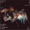 |
Fig. 1 Massive stars in the N11 B star-forming region in the LMC. The colour-composite image covers most of the stellar complex, and is formed using HST/WFPC2 filters in F656N (Hα), pseudo-green, and F502N ([O III]) as red, green, and blue components, respectively. We indicate the location of the complete sample of stars from Parker et al. (1992), identified as O-type stars (cyan), B-type (magenta), and unclassified objects (green). The eight ULLYSES targets studied here are identified by dashed circles with their respective ID numbers from Parker et al. (1992) and Evans et al. (2006). Scale and orientation are indicated. As a reference, LH 9 (Lucke & Hodge 1970) at the center of N11 is located to the south. |
2 Spectroscopic data
Our sample of O-type stars in N11 B is made up of ULL- YSES targets, and their spectra are publicly available to the scientific community1. These targets are: (1) PGMW 3053, (2) PGMW 3058, (3) PGMW 3061, (4) PGMW 3100, (5) PGMW 3120, (6) PGMW 3168, (7) PGMW 3204, and (8) PGMW 3223. In Table 2, we list the general information for each star, including magnitudes and extinction from this study, their known spectral types, radial velocities, and binarity status. These objects have been observed with HST, either with the Space Telescope Imaging Spectrograph (STIS) (Woodgate et al. 1998); or the Cosmic Origins Spectrograph (COS) (Green et al. 2012). In the Appendix (see Data Availability), we list the spectroscopic observations used in this work, obtained from different instruments, including relevant information on the covered spectral range, spectral resolution, observation dates, exposure times, and S/N.
The ULLYSES targets have complementary observations in the optical range provided by the X-shooter instrument (Vernet et al. 2011) on the VLT, which are key for our analysis. X- shooter covers the UV-Blue (UVB: 3000–5595 Å), visible (VIS: 5595–10 240 Å), and near-infrared (NIR; 10 240–24 800 Å). NIR spectra are not used in this work. We use X-shooter final products, which are flux- and wavelength-calibrated spectra provided by the data-reduction group of the XShootU collaboration (see Sana et al. 2024, for details), except for PGMW 3061 and PGMW 3204, as the final products for these objects have not yet been delivered. For these two targets, we retrieved the spectra from the ESO Science Archive Facility2. Three objects, PGMW 3053, PGMW 3120, and PGMW 3223, also have spectra from the Far Ultraviolet Spectroscopic Explorer (FUSE) satellite (Moos et al. 2000; Sahnow et al. 2000) with medium resolution (MDRS) in the UV range of 905–1187 Å. We use this information to complement our analysis. Additionally, seven targets (i.e., all apart from PGMW 3120) have GIRAFFE multiepoch spectra. GIRAFFE is a medium- to high-resolution (R = 5500–65 000) spectrograph in the optical range of 3700–9000 Å (Pasquini et al. 2002). We used these observations to check for binarity in Sect. 3.2.
In Fig. 1, covering most of N11 B, we indicate the brightest objects, complete at V < 16 mag from Parker et al. (1992), which are identified as O-type stars, B-type stars, and unclassified objects. The ULLYSES targets studied here are indicated.
Sample of ULLYSES targets. O-type stars in the N11 B star-forming region in the LMC.
3 Analysis
In order to model the observed spectra of the stars, one needs to follow a sequence of steps, as follows: (1) Determine the luminosity and extinction of the object, prioritizing recent Gaia DR3 photometry. (2) Check for binarity using available multiepoch spectra. (3) Determine rotational and “macroturbulent” velocities before fitting the spectral line widths. (4) Model the spectra to obtain the physical parameters of the stars. This process is done iteratively. Final stages include the determination of chemical abundances and X-ray luminosities, and refinement of the entire set of parameters comprehensively. We describe these different parts of our analysis below.
3.1 Bolometric luminosity and extinction
To determine the luminosity of our stars, we need to match the continuum of the synthetic spectrum of a selected model with the available photometry on the spectral energy distribution (SED). Reliable photometric values in the UV and optical ranges were taken from multiple references in the literature for the U, B, V, and R filters. Moreover, Gaia DR2 and DR3 values were included. In the NIR, we use the J, H, and K bands. In Sect. 5, we list the photometric values from different references used in this work to construct the SEDs of the analyzed stars in N11 B. Although we make use of most of the values available from the literature for UV up to the NIR, those values coming from Gaia (Gaia Collaboration 2018; Gaia Collaboration 2023) are prioritized in the optical range. In the UV range, the calibrated fluxes from HST COS and STIS can help as a photometric reference. Additionally, a careful inspection of each object was conducted using HST /WFPC2 images in filters F656N and F502N to ensure that we are considering the flux of a single object at the spatial resolution of HST (with a pixel scale of 0.05 arcsec/pixel). However, we did not use these filters to obtain extra photometric values, as these bands correspond to Hα (F656N) and [O III] (F502N), which are impacted by the nebular environment of the stars.
We note that in the case of the spectra obtained with X-shooter, using slits of 0.7 and 0.8 arcsec × 11 arcsec in the UVB and VIS ranges, respectively, we are observing single objects for PGMW 3053, PGMW 3061, PGMW 3168, PGMW 3100, PGMW 3204, and PGMW 3058. This is clearly not the case for PGMW 3223, where at least a second object as bright as our target star is inside the apertures of X-shooter, and a third one (although dimmer) is inside the aperture of FUSE. Thus, care must be taken when interpreting these values in the SED. The same is true for PGMW 3120, which has three objects inside the X-shooter aperture and two more (though dimmer) inside FUSE. On the other hand, HST COS and STIS apertures only cover the star of interest, and for this reason their fluxes can be considered reliable references to construct their SEDs. Figure 2 shows a zoomed-in view of 1 arcsec (0.24 pc at the distance of N11) in HST /WFPC2 images for the sample stars with their respective apertures from different instruments. Isocontours of brightness are used to inspect these images for probable contamination, like other spurious sources inside the slits covering our targets.
Once these aspects were taken into consideration, the construction process of the SED is as follows: first, the flux continuum of the model is scaled to the distance of the object. We assumed the same distance for all the objects, which is that of the LMC. Next, the reddening is determined by matching the slope of the SED, which is particularly sensitive towards the bluer wavelengths. We take into account the extinction attributed to the Galactic foreground (E(B – V)= 0.04 mag) and the LMC law. For this purpose, we used the reddening laws by Seaton (1979) and Trundle et al. (2007, for the LMC). The values we obtain are listed in Table 2 (columns 6 and 7). These values are better constrained than previous results in the literature, as we also used the flux levels of novel spectra in the UV range to determine the extinction and the luminosity of the stars. Detailed information on these differences is given in Sect. 5 for each star.
3.2 Checking binarity status
When studying massive stars, two possible scenarios must be considered for their evolution: the single (Conti et al. 1983) and the binary pathway (e.g., Vanbeveren et al. 1997). As most of the massive stars are expected to be in a binary or multiple star system (Sana et al. 2012), it is important to verify any indication of a binary companion before determining the stellar parameters as if we were dealing with a presumably single object. In order to check for binarity, multi-epoch spectra are required.
Our targets have multi-epoch observations from GIRAFFE. Although planned for other scientific cases, they allow us to check whether there is evidence of binarity, at least within the observed time frames, with the same resolution, exposure time, and S/N. The observed time periods span from 1 day to 1 month. However, the available observations are complex, and they need careful treatment for proper interpretation. For instance, the multi-epoch dates are different for each spectral range; for example, the observed time period spans 45 days for the spectral range of 3850–4050 Å; 24h for 4030–4200 Å; the same 24h for 4180– 4400 Å; a different 24h period for 4340–4340 Å; another 24h period for 4540–4760 Å, and 31 days for 6300–6690 Å. Details are provided in the Appendix (see Data Availability). With this information, we checked for binary features with orbital periods matching the duration of the available observations.
Here we check for any evidence of binarity in our sample. However, as well established, it is not possible to prove that a star is single. Even a lack of evidence of binarity does not necessarily mean it is not a binary. What we mean here by evidence of binarity includes radial-velocity shifts for SB1 types and variations in the line profile for SB2 types, such as double lines. Also, the presence of a companion does not necessarily dominate the key features of the spectrum of the star, and this depends on its physical parameters. According to our analysis, PGMW 3053 displays a variable He II λ4686 profile within a one-day time interval, as previously noted by Evans et al. (2006). We attribute these features to wind variability, and not to binarity. Other He II lines do not show variability. PGMW 3223 was found to be a binary. Its double line profile of He II λ4686 could be interpreted as a SB2 feature. However, no other He II lines display this characteristic feature. We classified it as SB1. The variability in radial velocity in the features of PGMW 3100 indicate a binary SB1. The remaining stars can be considered single, with the precaution mentioned above. Table 2 (column 11) lists the binary status of our sample.
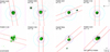 |
Fig. 2 Images of the LMC N11 B O-type stars, from HST/WFPC2 in the F656N filter (Hα), except for PGMW 3120 (HST/ACS/F220W). The ULLYSES targets are identified with their respective IDs from Parker et al. (1992, PGMW #) and Evans et al. (2006, N11 #). The slits from different instruments are indicated, including their shapes, sizes, and position angles: FUSE FUV/MRDS (dashed magenta; 4 × 20 arcsec); HST COS (dashed cyan; D2.5 arcsec); HST STIS/E140M (black rectangle; 0.2 × 0.6 arcsec); STIS/E230M (yellow square; 0.2 × 0.2 arcsec); GIRAFFE (dashed blue; D1.2 arcsec); X-shooter UVB (dashed red; 0.8 × 11 arcsec); and X-shooter VIS (red; 0.7 × 11 arcsec). Isocontours of brightness are displayed (green) to check for multiple sources inside the slits. Scale and orientation are indicated. |
3.3 Rotation
In order to determine the projected rotational velocity (3 sin i) of the stars, one ought to measure the broadening of their photospheric lines in absorption. Unlike the Balmer and He lines, the broadening of metal lines is normally attributed to macroturbulence rather than pressure. However, metal lines are generally weaker than H and He lines – or even absent – when insufficient S/N is obtained. Thus, dedicated observations should be analyzed when determining this parameter. Here, we use iacob-broad (Simón-Díaz & Herrero 2014), a standard semiautomatized tool to measure v sin i in OB stars (e.g., Holgado et al. 2018; Berlanas et al. 2020). This tool employs the Fourier transform (FT) and goodness-of-fit (GOF) methods. Briefly, the model spectra are convolved to the instrumental resolution of the analyzed spectra, and the rotational velocities are obtained. The values we report are the current rotational velocities at the equator multiplied by the sine of the inclination towards the observer, with this latter being an unknown parameter with the available data.
As an example, in Fig. 3 we show the graphical output obtained from the iacob-broad tool for a particular metal line in absorption of the PGMW 3053 star. The plot is rich in information. Briefly, the line profile of the selected metal, in this case N III λ4515 (in the upper left), is shown with different fittings from the two different methods: (1) FT, and (2) GOF with their projections, for “macroturbulent” velocity (vmac) to the left, and for the rotational component (3 sin i) in the top-right of the plot. There are four different fittings indicated with different colors: (1) red indicates the v sin i corresponding to the first zero of the FT; (2) blue indicates v sin i and vmac obtained from GOF; (3) green indicates the v sin i from the GOF, if vmac is assumed to be zero; and (4) purple shows the fitting of the vmac from the GOF, assuming v sin i is the first zero of the FT. We select the values from the last assumption, given it provides the best fit of the observed line, considering both vmac and v sin i contributions simultaneously.
We use exclusively metal lines in absorption to determine their v sin i broadening component. The metal lines we use are N III λ4515 (for PGMW 3053 and PGMW 3058). When N III lines are too weak or absent for a particular object, we check for more intense and resolved lines present in its spectrum. Though weaker, we use higher ionizing state N lines, such as N V λ4603.8 and N V λ4619.9, when N III is not detected (e.g., in PGMW 3061). Other metal lines are also used as well. We used Si IV λ4088.9 (for PGMW 3168) and C IV λ5801 (for PGMW 3100, PGMW 3120 and PGMW 3204). When using N III to determine rotation, we prioritize N III λ4515 over N III λ4518, given the latter is usually weaker and more difficult to fit. The same case applies for Si IV; Si IV λ4088.9 is usually stronger than Si IV λ4116.1, and sometimes Si IV λ4116.1 is even in emission. We do not use lines in emission to determine v sin i. Carbon lines also help, in the case of C IV, C IV λ5801 is prioritized over C IV λ5811, which is usually weaker. Oxygen lines like O III λ5592.3 also help (e.g., for PGMW 3223). We report our results for v sin i in Table 3. The iacob-broad tool provides computational errors for v sin i and vmac of around 5%. However, we assumed a value of 20% to account for errors associated with the methodology. This represents the lower error, and the upper error is consistent with the difference between v sin i (GOF) and v sin i (FT). Detailed information, like equivalent width (EW) and S/N, is given in Sect. 5 for the selected lines of each star.
We note that the iacob-broad tool determines the broadening of a given photospheric line, separating the contribution from two different effects: rotational broadening and non-rotational broadening. Rotational broadening is the v sin i parameter. On the other hand, non-rotational broadening, generally assumed to be macroturbulent broadening, is less understood. In fact, the given name is not necessarily related to the physical meaning of the term macroturbulence. Indeed, Simón-Díaz et al. (2017) explain how this name was originally introduced in the framework of cool stars; it is defined as “large-turbulent motions of material in the line-forming region” in that context. Here we aim to measure v sin i in order to study an invoked correlation between this parameter and the chemical enrichment of the stars (see Sect. 4.4). However, we also report the non-rotational broadening, referred to here as vmac for simplicity, because this broadening effect is important. Its contribution may even exceed the rotational velocity term (see e.g., Simón-Díaz et al. 2017; Holgado et al. 2018), and therefore it ought to be considered in the modeling of the spectra, independently of its physical meaning. Otherwise, by assuming vmac = 0 km s–1, we may be overestimating v sin i.
Discussing the physical origin of the non-rotational broadening in our stars is beyond the scope of this paper. However, we refer the reader to the detailed study by Simón-Díaz et al. (2017). Briefly, these authors conclude that the so-called macroturbulence can be attributed to pulsational modes related to a heat-driven mechanism and/or cyclic surface motions resulting from turbulent pressure instabilities in subsurface convection zones. Most of our stars have an important macroturbulent contribution, which has to be considered in our modeling. Reporting this value is also helpful for reproducibility and future reference. The vmac/v sin i ratios we find here are consistent with the findings of Simón-Díaz & Herrero (2014).
Finally, we also determine the v sin i parameter using the He I and He II lines. However, even for the same star, we obtain different values from those obtained with metal lines. This is not surprising, because as previously mentioned, other broadening (no-rotational) mechanisms start to play a role. Thus, we avoid using these lines to determine v sin i; indeed, H and He should only be considered for a rough estimation of rotational broadening when no metal lines are present.
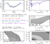 |
Fig. 3 Graphical output from the iacob-broad semi-automatized tool to determine projected rotational velocity (3 sin i) and non-rotational broadening. The example shown is for the star PGMW 3053, using the metal line of N III λ4515 in absorption. Five panels are displayed: (upper left) the line profile of the line; (upper right) the Fourier transform (FT) of the line; (lower right) 2D χ-distributions resulting from the Goodness-of-fit (GOF) analysis, and their projections (middle and lower left). The fitting in red indicates the v sin i corresponding to the first zero of the FT; the blue indicates the result for v sin i and “macroturbulent” velocity (vmac) from GOF; green indicates the result for v sin i from the GOF, if vmac is assumed to be zero; and purple shows the vmac from the GOF assuming v sin i is the first zero of the FT. The equivalent width (EW) and S/N measured in the neighboring continuum of the line are also indicated. In this case, EW = 50 mÅ and S/N = 196. Here, we take the v sin i value determined with the FT, and the vmac from the GOF, the fitting of which is shown in purple. Thus, for this star, we report v sin i = 88 ± 4 km s−1, and vmac = 15 ± 4 km s–1. |
Broadening parameters of the O-type stars in N11 B.
3.4 PoWR models
After determining key parameters such as L*, E(B – V), and v sin i, and checking for binarity in each of our objects, we then proceeded to model the observed spectra. We started by using synthetic spectra from the OB model grids by Hainich et al. (2019) generated with the PoWR model atmosphere pro- gram3. PoWR models are the simulated emergent spectra of hot stars with specified stellar and wind parameters, which consider nonlocal thermodynamic equilibrium (NLTE) radiative transfer, spherical symmetry, stationary outflow, metal line blanketing, and wind inhomogeneities. The rate equations for statistical equilibrium and radiative transfer are solved simultaneously by the PoWR code in the co-moving frame and secure energy conservation (see Gräfener et al. 2002; Hamann & Gräfener 2003; Sander et al. 2015, for more details).
Next, we calculated new synthetic spectra to model the stellar and wind parameters of our targets. The basic input parameters of a specific stellar model are the bolometric luminosity L⋆ and the stellar temperature T⋆. These are related to the stellar radius R⋆ via the Stefan-Boltzmann equation. The stellar radius is defined at a Rosseland-mean optical depth of 20. While T⋆ is the effective temperature related to that radius, one can also define an effective temperature Teff or T2/3, which is related to the radius where the Rosseland-mean optical depth reaches 2/3. For the types of atmosphere considered in this paper, the difference between T⋆ and Teff is negligibly small. Further fundamental parameters of a model include the surface gravity log g, the abundances, and the wind parameters (mass-loss rate M and terminal wind velocity v∞). The modeling procedure is described in Sect. 3.5.
For establishing the NLTE population numbers, the radiative transfer is calculated assuming the same Gaussian profiles in the absorption coefficient, with the width set equivalent to a Doppler velocity of 30 km s–1. This is a usual procedure and should account for turbulence, pressure broadening, and multiplet splitting of lines, which are not accounted for at this stage. For the hydrostatic equation in the quasi-static part of the atmosphere, we adopt a turbulence pressure (vmic) corresponding to 20 km s–1 (Shenar et al. 2016). When the model stratification has been established, the emergent spectrum is calculated in the observer’s frame of reference. Here, detailed line broadening is taken into account, and multiplets are split into their components. A microturbulence velocity (ξ) of 14 km s–1 is found to give adequate results (e.g., Hainich et al. 2019). In the wind, we tentatively adopt an additional contribution to ξ of 10% of the local wind speed. We used a clumping factor, or density contrast (D) of 10 (filling factor fV = 0.1), as described in Hamann & Koesterke (1998). We assumed a wind velocity field following the β-law from Castor et al. (1975), with the exponent β = 0.8, which is a typical value for O-type stars (e.g., Kudritzki et al. 1989; Repolust et al. 2004).
We included the following atoms in our analysis: H, He, C, N, O, Mg, Si, P, S, Fe, and Ni. The mass fractions for these elements are adopted from Trundle et al. (2007, for the LMC). The H (XH) and He (XHe) mass fractions are set to 0.738 and 0.258, respectively. The total CNO value is conserved, unless otherwise specified. When certain spectra need a different abundance (e.g., N enrichment), the relative values of these elements are changed accordingly. We start with typical mass fractions for CNO elements of: XC = 4.7 × 10⁻⁴, XN = 7.8 × 10⁻⁵, and XO = 2.6 × 10⁻³. The values for magnesium and silicon are XMg = 2.1 × 10⁻⁴ and XSi = 3.2 × 10⁻⁴, respectively. As there are no direct abundance measurements of phosphorus in the LMC (see e.g., Massa et al. 2003), P is set to 0.5 ZΘ, assuming a solar abundance from Asplund et al. (2009). The same is done for sulfur. The values for P and S are set to: XP = 2.9 × 10⁻⁶ and XS = 1.5 × 10⁻⁴, respectively. The iron group elements (from Sc to Ni) are treated with the super-level approach from Gräfener et al. (2002). For Fe, the adopted value is XFe = 7.0 × 10⁻⁴. Dielectronic recombination and autoionization mechanisms were taken into account for CNO ions. PoWR can also consider embedded X-rays, and they were included to model UV features.
Physical parameters obtained with PoWR models for the eight exemplary ULLYSES target O-type stars in N11 B.
3.5 Modeling the observed spectra with PoWR
Although the stellar and wind parameters of the O-type stars can be determined by specific diagnostic lines separately, it is important to note that these are not independent of each other, and thus all the lines of the spectrum, from the UV to the optical, should be addressed comprehensively. In this work, we used multiwavelength observations to model the sample of ULLYSES targets in N11 B. We analyze spectra from FUSE/MRDS, HST/STIS, and HST/COS in the UV, and from VLT/X-shooter in the optical. Given the multiwavelength spectral coverage, along with information on distance, precise photometric magnitudes, radial velocities, projected rotation, and extinction, we can construct the SED of each star and determine its bolometric luminosity. Next, we need to model the spectra of the stars. We start with prior groundwork. First, we chose synthetic spectra from the grid of PoWR models in the T⋆–log g plane by Hainich et al. (2019). Then, we chose the one with the closest T⋆ and log g to our spectra. Subsequently, specific lines and their profiles were carefully examined to recalculate new models and better model the key lines for each physical attribute. This process was carried out iteratively. Below, we explain the determination of each parameter.
The effective temperature (T⋆) of the stars is determined by modeling the He lines (e.g., He I λλ3819.6, 4120.8, 4471.5, 4713.1, 5015.7, 5875.6, 6678.1, 7065.2, and He II λλ3813.5, 4200.0, 4541.6, 5411.5, 6074.2, 6118.3, 6170.7, 6233.8, 6310.8, 6406.4, 6528.0, 6685.0, 6890.9, 7177.5, and 7592.7), and specifically the He I/He II ratio. The pairs He I λ3819.6–He II λ3813.5 and He I λ4471.5–He II λ4541.6 are particularly useful for this diagnostic. Except for He II λ4686, which is known to be mostly sensitive to the strength of the stellar winds of the stars. He II lines in the UV are also considered (e.g., λ1640.4). He II λ1085 is in principle covered by FUSE, although it is not useful given that other lines in absorption might be present in that range. Singlet lines of He I (1s2p P) at 4387.9 and 4921.9 Å have shown to be problematic in previous studies (see e.g., Najarro et al. 2006), and the reason for this remains unclear in the community. Thus, these lines were not considered for T⋆ determination.
The gravitational acceleration at the surface of the stars (log g) can in principle be determined by modeling the wings of the H-Balmer lines, as they are expected to be pressure- broadened by the Stark effect. However, care must be taken with Hα, as it is also sensitive to stellar winds. Therefore, mainly the lines of Hβ, Hγ, Hδ, Hϵ, and H9–H17 were considered to determine this parameter. The rotational and non-rotational broadening determined from the metal lines present in the spectrum (see Sect. 3.3) must be considered before determining the surface gravity; otherwise, log g is susceptible to overestimation. As T⋆ and log g are intrinsically correlated parameters and cannot be determined independently, they ought to be modeled simultaneously.
The main diagnostic lines for the wind mass-loss rate (Ṁ) in the optical range are typically Hα and He II λ4686. In the UV range, N V λλ1238.8, 1242.8 and C IV λλ1548.2, 1550.8 are particularly sensitive to the wind. The terminal wind velocity (v∞) is determined from the blue edge of the C IV λ1548.2 in absorption. The obtained parameters of the stars are given in Table 4.
We initially assumed standard LMC abundance values for C, N, and O. However, we need to change these values to better model certain metal lines. The abundances of the remaining elements are, in principle, fixed for all the stars. In the UV, the following lines were used: C III λλ1175.3, 1175.7; C IV λλ1548.2, 1550.8; and N III λλ1183.03, 1184.51, and 1751.7. When present, the following lines were considered in the optical range: C IV λλ5801, 5812; N III λλ4097.4 (although it is blended with Hδ), 4510.9, 4514.9, and 4518.149; and O III λ5592.3. Modeling the lines of N III λλ4634.1, 4640.6 in emission was found to be problematic and these lines were therefore not considered in the determination of nitrogen abundance; they are also sensitive to other parameters, such as the T⋆–log g of the stars. The effects of other parameters, such as the β-law, need to be explored to model these features. The CNO abundances by mass fraction and number are reported in Table 5. The errors were estimated by varying the abundances in test calculations. Values outside the given error range lead to a clear discrepancy between the model and the observations. We corroborated that our results do not change using the low-temperature dielectronic recombination (LTDR) approach. We refer the reader to the PoWR code manual (ManPoWR, Dec. 2013) for more information on this issue.
Furthermore, non-photospheric continuum emission originating from shock-heated plasma in the stellar wind of stars also leaves a significant imprint in the UV range of their spectra. Some of these features, such as N V λλ1238.8, 1242.8 and O VI λλ1031.9, 1037.6, are produced by X-rays and therefore need to be included for a complete modeling of the UV spectra. This can be achieved with PoWR. For this, three parameters were defined: (1) the fraction of electrons in the plasma phase (xfill); (2) the X-ray temperature (TX); and (3) the minimum radius at which the shockwaves occur (rmin). We note that by including X-rays, energy conservation might be compromised. Therefore, X-rays are included in the modeling process once we have obtained a converged model that is considered “final”, with its temperature stratification already defined, and reproducing the main stellar and wind features of the star. We report the ratio between X-ray and bolometric luminosity (LX/Lbol) for the O-type stars in Table 6. Uncertainties are estimated to be around 0.3 dex of the reported values. As usual, Lbol is defined as referring to the wavelength range below λ = 40 Å (≈ 0.3 keV).
Additionally, a correction for the expected ISM absorption by the hydrogen Lyman lines (Lyα and Lyβ) present in the observed UV range was included in our models. For this, the color excess for both the Galaxy and the LMC was considered, along with the radial velocity. The column density (NH) of the local ISM was determined using NH = 3.8 × 1021 cm s–2 E(B – V), following Groenewegen & Lamers (1989).
An example of the PoWR model for one of the stars in our study, PGMW 3053, is shown in Fig. 4. The first panel shows the constructed SED. The second panel shows the FUSE UV spectrum normalized to the continuum model. The key stellar lines are indicated, and when present, nebular emission lines and interstellar (i.s.) atomic and metal lines in absorption (listed in Haser et al. 1998, Table 4) are also labeled. Strong ISM molecular hydrogen absorption lines are particularly present in this range; they are also indicated, although their modeling is outside the scope of this work. The third and fourth panels show the HST /COS UV spectrum normalized to the continuum model. The normalized line spectra of wavelength ranges with key lines of H, He, and metals are shown in Figs. 5 and 6. The corresponding modeling for the rest of the stars is shown in the Appendix (see Data Availability).
CNO abundances for the O-type stars in N11 B.
X-ray parameters for the O-type stars in N11 B.
Stellar parameters obtained with BONNSAI.
3.6 Evolutionary masses and ages
We used the BONNSAI web service4 (Schneider et al. 2014) to obtain the predicted evolutionary mass (Mev), age, and initial rotation of the stars. For this, we introduce a list of stellar parameters previously determined with PoWR modeling: L⋆, T⋆, and log g. We also determined the v sin i with the iacob-broad tool.
BONNSAI assumes main sequence single stars with initial stellar masses (Mini) of between 5 and 5000 M⊙, initial rotational velocities (vini) of between 0 and 600 km s–1, and a power-law initial mass function (IMF) with a slope of γ = –2.35 from Salpeter (1955). Stellar models by Brott et al. (2011) and Köhler et al. (2015) were chosen for the LMC. The replicated observables with BONNSAI, T⋆, log g, L⋆, and v sin i, are given in Sect. 5 for each star. The results are reported in Table 7. These values must be interpreted with caution, as in some cases, the replicated observables do not precisely match the stellar parameters determined with PoWR models, but rather represent a similar set of parameters (the closest values) from their grid of models. Any such differences are discussed later in the text.
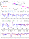 |
Fig. 4 PoWR model for the star PGMW 3053. The observed spectrum is shown by a blue line and the model by a red dashed line. (First panel) SED with photometric magnitudes (colored boxes). The UV spectra better constrain the E(B − V) and L⋆ of the star (also indicated at the upper right, among other parameters). The widths of the Gaia DR3 filters (blue, central, and red arms) are also indicated. (Second panel) FUSE/MRDS UV spectrum normalized to the continuum model. (Third and fourth panels) HST/COS UV spectrum normalized to the continuum model. The terminal velocity (v∞) is determined from the blue edge of the C IV line in absorption. Nitrogen enhancement is determined with N III at 1183 and 1185 Å, also considering these ions in the optical range, and the carbon abundances is determined using C III at 1175 and 1176 Å in the UV. The N V λλ1238.8,1242.8 and O VI λλ1031.9,1037.6 features are particularly sensitive to X-rays. We also considered ISM absorption features by the hydrogen Lyman lines in our modeling. Interstellar (i.s.) atomic, molecular, and metal lines in absorption are indicated. The legend “fudge” means that the FUSE spectrum had to be scaled by 1.2 for comparison purposes in the second panel. There is a gap of around 10 Å in the observations around 1090, 1280, and 1605 Å, where no key lines are present. See text for details. |
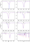 |
Fig. 5 PoWR model for PGMW 3053. Several windows are displayed to show the Balmer lines present in the observed spectrum in detail: Hα, Hβ, Hγ, Hδ, Hє, and H10–H17, in comparison with the final model of the star. The surface gravity (log g) parameter of the star is determined from the wings of the H lines. In this particular case, Hγ is the optimal line to use, given that it is not blended with other lines (e.g., Hβ, Hδ, Hє), and is also more intense than H8–H17. Hα is the most intense H line, although it is sensitive to the stellar winds and is therefore considered to determine mass-loss rate (Ṁ). The Hα line is affected by a strong feature in absorption, most likely by the nebular emission subtraction. The observed spectra are shown by a blue line and the PoWR model by a red dashed line. The most important lines are identified. |
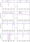 |
Fig. 6 PoWR model for PGMW 3053. Several windows are displayed to show the most important He I and He II lines, as well as some metals, in comparison with the final model of the star. The temperature (T⋆) of the star is determined by modeling the He I-He II ratios (e.g., He I λ4471.5, and He II λ4541.6). Singlet lines of He I (1s2p P) at 4387.9 and 4921.9 Å are identified with blue labels and were not used for diagnostic. Non- photospheric lines (e.g., Na) and features in absorption ([O III]), most likely due to nebular emission subtraction, are indicated with green labels. He II λ4686 is crucial for determining the mass-loss rate (Ṁ) of the star. Rotational broadening and chemical abundances, such as that of nitrogen, are determined from metal lines in absorption (e.g., N III λ4515 and N III λ4518). The observed spectra are shown by a blue line and the PoWR model by a red dashed line. The most important lines are identified. |
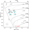 |
Fig. 7 Hertzsprung-Russell diagram for the sample of ULLYSES target O-type stars in N11 B. Evolutionary tracks (continuous lines) and isochrones (dotted lines) from Brott et al. (2011) and Köhler et al. (2015) with LMC composition are displayed. The ULLYSES targets (cyan circles) are identified with the PGMW # from Parker et al. (1992). The stars have ages of between 2 and 4.5 Myr, and evolutionary masses of 25– 45 M⊙. The ZAMS line, and the completeness threshold of V> 16 mag are displayed (red line). Typical uncertainties are indicated. |
4 Discussion
4.1 Stellar parameters
A sequential star-formation scenario has been suggested by Parker et al. (1992) to explain apparent gradients of age and extinction, and even the IMF slope, from the central nebular cavity in N11 (named LH 9) to the surrounding star-forming complexes, among which N11 B is the most prominent H II region. In LH 9, Parker et al. (1992) derived an age of 5 Myr, and a reddening of E(B − V) = 0.05 mag. The low value of the visual extinction could suggest a low gas density, with the gas probably being lost due to stellar winds. WR stars are known for their strong stellar winds (Crowther 2007), and indeed at the very center of LH 9 lies an extended source hosting a WR system (WC4+09.5II; Bartzakos et al. 2001), consistent with the low gas density and the age of the region. On the other hand, N11 B is thought to be ~2 Myr younger, and with three times higher extinction. No WR sources have been found in N11 B.
After obtaining L⋆ and T⋆ for our targets, we determined the ages and masses using a Hertzsprung-Russell (H-R) diagram (see Fig. 7). Evolutionary tracks and isochrones from Brott et al. (2011) and Köhler et al. (2015) were used for the LMC. We find that the O-type stars in N11 B are located among isochrones for ages of 2–4.5 Myr. The young age of this region is consistent with a pre-WR phase (<4 Myr). No SNRs have been observed in this region so far. We report an age difference of ~2 Myr between the stars analyzed in N11 B and those located in the central region. Additionally, according to the evolutionary tracks, the stellar masses are within 25–40 M⊙. We report a median value for extinction of E(B − V) = 0.19 mag in N11 B.
When comparing the spectroscopic masses (Mspec) obtained with PoWR with the evolutionary values (Mev) derived with BONNSAI (see Fig. 8), we notice that the stars do not follow a clear one-to-one relation, particularly above Mspec~55 M⊙. Stars with Mspec~20–45 M⊙ have Mev of within 25–40 M⊙. However, for some stars, Mev is higher than Mspec by ~10 M⊙. This is the case for PGMW 3053, PGMW 3168, PGMW 3100, and PGMW3058, with PGMW3061 (and Sk −66° 171) being the exception. On the other hand, stars with Mspec of 55-65 M⊙ have Mev of within 30–40 M⊙. The values for Mev are lower than Mev by ~20 M⊙. This is the case for PGMW 3120, PGMW 3204, and PGMW 3223. We note that PGMW 3120 was found to be a member of a cluster of at least three stars, and PGMW 3223 is likely a binary SB1. This is not the case for PGMW 3204, the third outlier in the plot, where no evidence of binarity has been found in GIRAFFE spectra. On the other hand, PGMW 3100 is also a binary SB1, but the mass discrepancy is rather small. Upon careful examination of the replicated values of BONNSAI, we note that log g and/or L⋆ are underestimated for these three objects, contributing to the lower Mev . The reason for this underestimation is the parameter space considered in the models used to predict the masses.
However, we also note that a discrepancy between Mev and Mspec has been reported for O-type stars (e.g., Herrero et al. 1992; Martins et al. 2012; Mahy et al. 2015; Ramachandran et al. 2018), and even for B-types (Bernini-Peron et al. 2024). The mass discrepancy obtained in this study presents yet another instance of this problem, which remains unsolved so far. In this regard, Mahy et al. (2020) suggested that stars that suffer from interaction present this discrepancy. The fact that this discrepancy is well observed and documented in the Magellanic Clouds reveals that it cannot be attributed solely to the determination of luminosities.
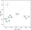 |
Fig. 8 Evolutionary (Mev) vs. spectroscopic (Mspec) masses for the analyzed O-type stars in N11 B. The Mspec values were obtained with PoWR modeling, and the Mev values were derived with BONNSAI by introducing PoWR-obtained parameters. The objects are indicated with their PGMW # ID. In addition, the two Sanduleak O-type stars (not in N11 B) also analyzed here are shown (green squares). A one-to-one relation is indicated (dashed line) as a reference. Triangles represent lower limits (see text for details). The gray color indicates confirmed SB1 binarity, and the member of a cluster is shown in black. |
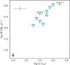 |
Fig. 9 Mass-loss rate (log Ṁ) vs. bolometric luminosity (log L⋆) for the O-type stars analyzed in N11 B. In addition, the stars Sk −66° 171 and Sk −69° 50 (not in N11 B) are also shown as references (green squares), as well as N11 046 (blue square). An increasing trend between M and log L⋆ is observed. Notations are the same as in Fig. 8. Typical uncertainties are indicated. |
4.2 Wind parameters
Determining the wind parameters of O-type stars is critical for establishing their feedback contribution and investigating the ecology of their local environment. In this study, we determine the mass-loss rate and other key wind parameters obtained not only in the optical range, but also from novel UV spectra from ULLYSES. The P-Cygni lines in the UV allow us to obtain the Ṁ parameter, together with the Hα and He II λ4686 lines. In Fig. 9, we note an increasing trend between the mass-loss rates and the luminosities of the O-type stars in N11 B. We determined log Ṁ values in the range of −6.7 to −6.0 M⊙ yr−1. Among our sample of stars, PGMW 3061 and PGMW 3053 have the highest massloss rates and are also the most luminous objects. On the other hand, PGMW 3168 has the weakest winds, being the least luminous star. This star also has the lowest log g and therefore the lowest mass of the sample. The additional stars analyzed here for the feedback section (Sect. 4.6) follow the same trend.
However, in order to discuss the strengths of the stellar winds, it is often more useful to use the modified wind momentum (Dmom) definition instead of Ṁ alone. For this, we used the expression from Kudritzki & Puls (2000) for Dmom, which is defined as  . By doing so, we can compare the parameters from the modeling of our observations with the theoretical wind-momentum–luminosity relation (WLR) predicted by Vink et al. (2000), and also the empirical WLR for LMC OB stars by Mokiem et al. (2007b). In Fig. 10, we plot Dmom versus luminosity for the analyzed O-type stars in N11 B. There is a clear increasing trend between these two parameters. Our observations are consistent with the WLR predicted by Vink et al. (2000). The empirical WLR for LMC OB stars by Mokiem et al. (2007b) is 0.2 dex above our results. Additionally, a linear regression of our values is shown in the form of y = a + b ⋅ x , with a = −15.5 and slope b = 2.4. Three objects (PGMW 3168, PGMW 3204, and PGMW 3223) lie below the WLR by Vink et al. (2000). In the present work, we confirm that PGMW 3223, which shows the greatest deviation from the relation, is an SB1 binary (see Sect. 5). However, the other two objects are likely single. We aim to include additional ULLY- SES targets being analyzed within the collaboration to report a robust WLR for the O-stars in the LMC.
Also displayed are the O-type stars Sk −66° 171 and Sk −69° 50 in the LMC as a reference. The physical parameters obtained with PoWR for Sk −66° 171 and Sk −69° 50 are reported in Sect. 5 with the purpose of quantifying the ionizing photons for stars of their subtypes. These two stars also follow the WLR relation by Vink et al. (2000), like the O-type stars in N11 B.
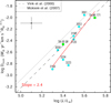 |
Fig. 10 Modified wind momentum (Dmom) vs. luminosity (log L⋆) for the O-type stars analyzed in N11 B. An increasing trend is observed. Two exemplary WLRs are displayed: the one predicted by Vink et al. (2000) (dashed line) and the empirical relation obtained for LMC OB stars by Mokiem et al. (2007b) (dotted line). Notations and color-coding are the same as in Fig. 9. Typical uncertainties are indicated. A linear regression of our values is shown by a red continuous line. |
4.3 X-ray luminosities
In binary systems, X-rays are expected to be produced either by the collision of stellar winds or by the accretion of the wind onto a compact object (Puls et al. 2008). The X-ray observations of massive stars in Oskinova (2005) indicate that the correlation between bolometric and X-ray luminosity known for single O-type stars also applies to O+O and WR+O binaries. There is currently no conclusive evidence to determine whether binary stars exhibit X-ray emission in excess of that of single stars. Low luminosities do not necessarily indicate the absence of a secondary companion. Also, there is still the possibility that the companion is in a quiescent state.
Using XMM-Newton observations, Nazé et al. (2004) reported diffuse emission and X-ray sources associated with the massive stars in N11 B. Later, with the more sensitive and higher spatial resolution of the Chandra X-ray Observatory, Nazé et al. (2014) investigated the point sources associated with the O-type stars in N11 and determined log(LX/Lbol) values between −6.5 and −7. Although several values are upper limits, these results led them to conclude that these stars are highly magnetic or are colliding-wind binary systems. Additionally, Crowther et al. (2022) showed that OB and WR stars in the Galaxy follow a relation of LX = 10−7 Lbol, which is compatible with the findings of Nazé (2009).
We included X-rays in our PoWR models to reproduce available spectral features in the UV. X-ray continuum emission from shock-heated plasma is expected to originate in the winds of the stars. The O-type stars analyzed here are not strong X-ray point sources according to Nazé et al. (2014). We list their log(LX/Lbol) values in Table 6. Nazé et al. (2014) reported upper limits for four of our objects: PGMW 3053, PGMW 3058, PGMW 3168, and PGMW 3223. Here, we report their log(LX/Lbol) values, as obtained using our spectroscopic modeling approach, independently of previous X-ray observations. With the exception of one of these sources, we obtained values below the upper limits reported by Nazé et al. (2014). The values for the rest of the sample are consistent with previous observations. We report the ratio between X-ray and bolometric luminosity log(LX/Lbol) for the O-type stars in Table 6, including the assumed xfill, TX, and rmin parameters. We should also keep in mind the variable nature of the X-ray sources, but we still lack the necessary multi-epoch UV spectra to study this matter. However, we conclude that the sample of massive stars in N11 B analyzed here is not made up of strong X-ray emitters. We find typical log(LX/Lbol) values for our targets in the range of −7.0 to −6.6, with the earliest star in N11 B, PGMW3061, exhibiting log(Lx/Lbol) = −6.6, making it the brightest X-ray emitter in the region.
4.4 Chemical abundances
It is commonly assumed that the faster the star rotates, the higher the rotational mixing, resulting in a higher N abundance in the surface of the star. However, for a sample of early B-type stars in the LMC, Hunter et al. (2008) already reported evidence contradicting this assumption. Among their findings, they show highly nitrogen-enriched slow rotators (<50 km s−1) and nitrogen-unenriched fast rotators (~300 km s−1), thus challenging the often-invoked rotational mixing hypothesis.
Interestingly, Maeder et al. (2009) suggest that it is not only rotation that plays a role in mixing, but also age, mass, and metallicity. Petrovic et al. (2005) proposed a scenario where nitrogen-unenriched fast rotators may be explained by a close binary companion increasing the rotation rate of the star. On the other hand, Wolff et al. (2007) suggested that this correlation originates early in the star formation process due to the magnetic locking of the star to the accretion disk, which is known as the fossil field hypothesis. However, we lack observations of magnetic field strength for our sample of stars. Previously, Brott et al. (2011) tested the rotational mixing hypothesis by simulating LMC massive stars. However, due to the lack of reported nitrogen abundances for stars with temperatures of greater than 35 kK, meaning that the O-types were almost completely excluded from their study, their results only apply to early B-type stars.
The chemical abundances of C, N, and O for the analyzed O-type stars in N11B are reported in Table 3. None of the studied objects can be considered a fast rotator (>300 km s−1), nor are they slow rotators. We note that the majority of the Galactic O-type stars analyzed by Holgado et al. (2018) have v sin i < 120 km s−1, with the distribution of v sin i reaching a maximum around 40–80 km s−1. Here, we report rotational velocities in the range of 55–143 km s−1, with a median value of v sin i = 100 km s−1, consistent with findings by Ramírez- Agudelo et al. (2013) in 30 Dor. None of the determined v sin i of our stars are higher than 150 km s−1 . Despite this fact, half of the targets do display N enrichment, up to a factor of 7, corresponding to 3.5 Z⊙. This is the case for PGMW 3053 and PGMW 3120. The surface nitrogen abundances that we find are comparable to the findings for LMC O-type stars by Ramachandran et al. (2018), showing a nitrogen enrichment of a factor of between 1 and 10 for most of their objects. In Fig. 11, we compare the surface nitrogen abundances (log(N/H) + 12) by mass and v sin i for the analyzed objects. Also in this figure, we indicate the non-rotational contribution (vmac) to the broadening for each star. According to these results, we cannot conclude that the nitrogen surface abundances of the stars are modified by the effects of rotational mixing.
We note that we were not able to model Si IV λ4088.9 or Si IV λ4116.1 when they are in emission. In our models, we obtain these features in absorption. However, reducing the Si IV abundance by a factor of 4 decreases the strength of the lines in absorption. We take note of this result for future analysis efforts.
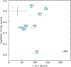 |
Fig. 11 Surface nitrogen abundances (log (N/H) + 12) by mass vs. projected rotational velocity (v sin i) for the O-type stars analyzed in N11 B. Most of the objects are nitrogen-enriched by up to a factor of seven. A standard nitrogen abundance in the LMC (log(N/H) + 12 = 6.88) is indicated as a reference. With a median value of v sin i = 100 km s−1, none of the stars are considered slow or fast rotators. The non-rotational broadening for each star (vmac) is also indicated with an empty circle. No trend is apparent. Typical uncertainties are indicated. |
4.5 Macroclumping
For the sake of simplicity, stellar winds of massive stars have been assumed to be homogeneous and stationary. Using PoWR models on UV observations, Oskinova et al. (2016) point towards highly inhomogeneous stellar winds. Phosphorus lines in the UV, P V λ1118 and P V λ1128 in particular, are considered mass-lossrate diagnostic features (Fullerton et al. 2006). However, there has been an observed discrepancy between the values obtained using these phosphorus lines in the UV and those obtained using only the optical diagnostic features. P V tends to appear weaker than expected based on its Ṁ determined using optical lines (e.g., Massa et al. 2003; Oskinova et al. 2016). In order to make sense of this discrepancy, Massa et al. (2003) point to three possible scenarios: (1) the Ṁ is lower than the values obtained using optical features (He II λ4686 and Hα); (2) the assumed phosphorus abundance is overestimated; and/or (3) the winds are strongly clumped. We explored these scenarios.
The effects of including macroclumping to solve this discrepancy have been discussed in Oskinova et al. (2016). Here, we use the macroclumping approach for the stars with FUSE spectra: PGMW 3058, PGMW 3223, and PGMW 3120. We confirm the effect of including macroclumping in the modeled P V lines. However, we also note that other spectral features are affected, indicating that this approach requires further investigation.
Massa et al. (2003) also remark that there are no direct measurements of the phosphorus abundance in the LMC, and that the Ne burning history may cause the trend in abundance to differ for phosphorus in the LMC. Thus, in this work, we considered this scenario to be worth exploring. We find that by reducing the abundances by a factor of four, the modeled P V lines can match the observed features for two of our objects with FUSE spectra: PGMW3058 and PGMW3223. We also note this effect in Sk −66° 171 and Sk −69° 50. This exercise has been explored in the past. Notably, Bouret et al. (2012) also had to decrease the phosphorus abundance to model the spectral lines with CMFGEN. Interestingly, the models for PGMW 3120 and N11 046, respectively, do not require either macroclumping or lower phosphorus abundance to match the P V features in the UV.
We should consider that if the iron abundances are also assumed to be around half solar, there would be no reason to speculate further on lower phosphorus abundances, as the two elements would be expected to follow the same trend. However, we take note of this result, which merits further exploration with ULLYSES targets in the LMC.
4.6 Stellar feedback
The main contributors to the feedback in star-forming regions are expected to be the hot and luminous OB stars –and particularly the WR population (see Crowther 2019)– and SNRs. In N11 B, there are no WR stars or even candidates, nor are there any known SNe yet. This could be attributed to the young age of the region (2–4.5 Myr). Thus, N11 B can be considered an exemplary environment in which to study the feedback contribution coming solely from its massive O-type stellar population. In this region, we find that two stars display the highest mass-loss rates: PGMW3053 and PGMW3061, both with a log(Ṁ/M⊙ yr−1) = −6.0, and the highest Dmom is found in PGMW 3061 (see Figs. 9 and 10).
Individual ionizing photons and the mechanical energy of the analyzed ULLYSES targets are reported in Table 3. The total amount of ionizing photons produced by the 25 O-type stars known in N11 B is also estimated. For this, the ionizing feedback for each of the O-type stars based on their spectral type (see Table 8) was considered to quantify the total ionizing feedback in the region. Stars of different spectral types in N11 B, particularly those of later subtypes, were not among the ULLYSES targets. We tackle this problem using Sk −69° 50, Sk −66° 171, and N11 046. Although these stars are not located in the region studied here, they share spectral classifications with some of the objects. Sk −69° 50, with a spectral type O7(n)(f)p, was used to estimate the ionizing photons of the only O7V star in N11 B: PGMW 3102. Sk −66° 171, with a spectral type O9 Ia, was used to estimate the ionizing photons of the O9.5III star PGMW 3045. N11 046, with a spectral type O9.5 V, was used to estimate the ionizing photons of five O9.5V stars, namely PGMW 3063 (O9V), PGMW3115 (O9V), PGMW3103 (O9.5), PGMW3016 (O9.5), and PGMW 3042 (O9.5Vn). Two stars, PGMW 3173 and PGMW 3264, are reported with uncertain spectral types between O4-O6V and O3-O6V, respectively. For these, the ionizing photons of a star with an intermediate spectral type were used, PGMW 3120a (O5.5V). Including these stars allows us to estimate the total ionizing photon fluxes Σ QH, P QHe I, and Σ QHe II produced by the 25 O-type stars in N11 B.
We estimate that the combined ionizing photon fluxes from the analyzed stars in N11 B are: QH = 3.0 × 1050 ph s−1, QHe I = 3.5 × 1049 ph s−1, and QHe II = 2.7 × 1044 ph s−1. If X-rays are taken into account, then QHe II = 5.9 × 1044 ph s−1, which is a factor of about 2 higher than without considering X-rays. We note that this estimate relies on the assumption that our stars share the physical properties of a given spectral type. The total Lmec is ΣLmec = 2900L⊙, with PGMW 3061 – the star of our sample with the earliest type – being the main contributor to the total amount of energy by almost half of the total mechanical luminosity, with Lmec= 960 L⊙. We find PGMW3058, an O3 V star, to be the main contributor in QHe II, with log QHe II= 43.5 ph s−1.
The Tarantula Nebula in the LMC is considered a reference for extragalactic H II regions. We compare our results with this region. Crowther (2019) list the contributions of very massive stars, early O-types, and WR stars to the Lyman continuum feedback in 30 Dor. Details of the census are reported in Doran et al. (2013). This complex is the brightest and most important cluster in the LMC, with 570 O-type stars, 523 B-type stars, and 28 WR stars. WR stars are the main contributors to ionizing feedback in this region (Crowther 2019, see their Table 4), each one producing an order of magnitude more ionizing photons than a single O-type star; the latter objects inject log QH~49 ph s−1 into their local environment. On the other hand, B-type stars are not expected to significantly contribute to ionizing feedback. Their contribution in mechanical energy could have an impact, considering that Lmec is driven by Ṁ and terminal velocity  . B-type stars in the SMC have roughly an order of magnitude lower mass-loss rates and terminal velocities that are two to five times lower (Bernini-Peron et al. 2024). While these regions host several “examples of stellar exotica” (Crowther 2019), N11 B is a region with a rather modest OB population, with neither WR stars nor supernovae yet, as mentioned above. However, we see precisely this property as an opportunity to quantify the feedback solely from typical O-type stars of different subtypes.
Pellegrini et al. (2012) reported L(Hα) = 1.023 × 1039erg s−1 for the N11 region, named MCELS-L65 or DEM L 34 in their catalogue, making it the second brightest H II region in the LMC, surpassed only by the 30 Dor nebula, which these authors refer to as MCELS L-328 or DEM L 263, and for which they report L(Hα) = 4.571 × 1039erg s−1. The luminosity reported by Pellegrini et al. (2012) in N11 corresponds to QH = 7.27 × 1050 ph s−1 , which is obtained using the expression QH = 7.1 × 10¹¹L(Hα) s−1 given by Kennicutt et al. (1995) to determine the number of Lyman continuum photons under Case B recombination and ionization-bounded nebula assumptions. Here, we estimated the ionizing budget in N11 B, which is the brightest star-forming region in N11. We report ΣQH = 3.0 × 1050 ph s−1. This value is consistent with the total budget of ionizing photons in N11.
Individual ionizing photons of the O-type stars in N11 B.
5 Conclusions
We investigated in detail the stellar parameters, wind features, mechanical, and ionizing feedback of eight ULLYSES targets: benchmark O-type stars with spectral types ranging from O2 to O8 and with different luminosity classes, in the N11 B starforming region in the LMC. We used state-of-the-art PoWR models and other standard analysis tools in a homogeneous approach. We analyzed novel UV HST/STIS and COS high- quality spectra from the ULLYSES project, as well as optical spectra from X-shooter at the VLT, along with the most recent Gaia DR3 photometry. We summarize our main findings as follows:
We report ages of between 2 and 4.5 Myr and masses of 30–60 M⊙ for the O-type stars analyzed in N11 B. Such young ages are consistent with the absence of WR stars, the fact that no SNe have been reported in this region yet, and with the hypothesis of a sequential star-formation scenario from the center of N11 to the surrounding regions;
We show that the Mev and Mspec do not follow a clear one- to-one relation. This mass discrepancy is consistent with previous findings in the literature (e.g., Herrero et al. 1992, in the Magellanic Clouds);
The analyzed O-type stars follow a wind-momentum- luminosity relation that is consistent with previously reported observational relations and with the theoretically predicted relation by Vink et al. (2000);
We investigated whether nitrogen enrichment correlates with v sin i. The O-type stars analyzed here have rotational velocities ranging from 55 to 143 km s−1, with a median value of 100 km s−1. Non-rotational components were considered. We observe nitrogen enrichment in most of the stars of up to a factor of 7. However, we do not find a trend with v sin i, challenging the hypothesis that nitrogen enrichment is correlated with rotation in massive stars;
The effect of “macroturbulence” on line broadening was found to be non-negligible. On the contrary, vmac is an important contributor and even dominates the line broadening in most cases. Our result is consistent with previous findings of Simón-Díaz et al. (2017) and Holgado et al. (2018). We recommend that its contribution to the total broadening of a line should not be ignored, and that the use of non-metallic lines for determining v sin i should be avoided, when possible. Additionally, we find that even for the same star, the metal lines give different values compared to those obtained with the Balmer and He lines. Therefore, these lines should be avoided when possible;
In the UV range, we observed that reducing the phosphorus abundances by a factor of four causes the modeled P V lines to match the observed lines, which is similar to the well- studied macroclumping effect;
By including X-rays in our PoWR models, we quantified the amount of X-rays required to reproduce important UV spectral features in our stars. We independently report LX/Lbol ratios of between −7.5 to −6.6, including for the first time the values for four O-type stars in N11 B. These values are consistent with soft-X-ray emitters and previous findings (Nazé et al. 2014; Crowther et al. 2022);
The fact that N11 B is free of “exotic” objects gives us the opportunity to study the ionizing feedback in a starforming region exclusively through its O-type stars. We report total ionizing fluxes of log(ΣQH) = 50.5 ph s−1, log(ΣQHe I) = 49.6 phs−1, and log(ΣQHe II) = 44.4 phs−1. If X-rays are considered, then log(ΣQHe II) = 44.8phs−1, which represents an additional 0.4 dex of ionization;
The total mechanical luminosity of the eight stars analyzed here is ΣLmec = 2900 L⊙. PGMW3061, the earliest analyzed star (ON2 III(f*)), is the main contributor, with log (Lmec/L⊙) = 3.0. It is a factor of 3–14 stronger in Lmec compared to the next brightest and faintest sources analyzed, respectively. PGMW 3061 is also the main contributor to QH and QHe I. PGMW 3058, an O3V(f*) star, is the main contributor to QHe II. Given the absence of WR stars and SNRs, the O-type stars alone provide the feedback in N11 B.
In summary, this work is part of a larger project, the aim of which is to determine the stellar and wind parameters of the OB stars in the ULLYSES sample. This study is among the initial steps in using PoWR models to achieve this goal in a homogeneous way.
The next step is to increase the sample size analyzed with PoWR and statistically compare the results with theoretical predictions. Here, we present the methodology required for this, including the analysis of novel UV spectra where key wind parameters are found, along with other features to constrain the stellar properties –in particular, more reliable luminosities and the extinction of the stars with UV fluxes and Gaia photometry.
Data availability
The appendix for the paper is available at: https://doi.org/10.5281/zenodo.14245532
Acknowledgements
This study is based on observations collected at the European Southern Observatory under ESO program 106.211Z.001. Observations obtained with the NASA/ESA Hubble Space Telescope were retrieved from the Mikulski Archive for Space Telescopes (MAST) at the Space Telescope Science Institute (STScI). STScI is operated by the Association of Universities for Research in Astronomy, Inc. under NASA contract NAS 5-26555. VMAGG is funded by the Deutsche Forschungsgemeinschaft (DFG - German Research Foundation), grant number 443790621. This work has made use of data from the European Space Agency (ESA) mission Gaia (https://www. cosmos.esa.int/gaia), processed by the Gaia Data Processing and Analysis Consortium (DPAC, https://www.cosmos.esa.int/web/gaia/dpac/ consortium). Funding for the DPAC has been provided by national institutions, in particular the institutions participating in the Gaia Multilateral Agreement. AACS, VR, and MBP are supported by the Deutsche Forschungsgemeinschaft (DFG – German Research Foundation) in the form of an Emmy Noether Research Group – Project-ID 445674056 (SA4064/1-1, PI Sander) and acknowledge funding from the Federal Ministry of Education and Research (BMBF) and the Baden-Württemberg Ministry of Science as part of the Excellence Strategy of the German Federal and State Governments. AuD acknowledges NASA ATP grant number 80NSSC22K0628 and support by NASA through Chandra Award number TM1-22001B and GO2-23003X issued by the Chandra X-ray Observatory 27 Center, which is operated by the Smithsonian Astrophysical Observatory for and on behalf of NASA under contract NAS8-03060. ACGM thanks the support from project 10108195 MERIT (MSCA-COFUND Horizon Europe).
References
- Abbott, B. P., Abbott, R., Abbott, T. D., et al. 2017, Phys. Rev. Lett., 119, 161101 [Google Scholar]
- Arellano-Córdova, K. Z., Berg, D. A., Chisholm, J., et al. 2022, ApJ, 940, L23 [CrossRef] [Google Scholar]
- Asplund, M., Grevesse, N., Sauval, A. J., & Scott, P. 2009, ARA&A, 47, 481 [NASA ADS] [CrossRef] [Google Scholar]
- Bartzakos, P., Moffat, A. F. J., & Niemela, V. S. 2001, MNRAS, 324, 18 [NASA ADS] [CrossRef] [Google Scholar]
- Berlanas, S. R., Herrero, A., Comerón, F., et al. 2020, A&A, 642, A168 [NASA ADS] [CrossRef] [EDP Sciences] [Google Scholar]
- Bernini-Peron, M., Sander, A. A. C., Ramachandran, V., et al. 2024, A&A, 692, A89 [NASA ADS] [CrossRef] [EDP Sciences] [Google Scholar]
- Bonanos, A. Z., Massa, D. L., Sewilo, M., et al. 2009, AJ, 138, 1003 [Google Scholar]
- Bouret, J. C., Hillier, D. J., Lanz, T., & Fullerton, A. W. 2012, A&A, 544, A67 [NASA ADS] [CrossRef] [EDP Sciences] [Google Scholar]
- Brott, I., de Mink, S. E., Cantiello, M., et al. 2011, A&A, 530, A115 [NASA ADS] [CrossRef] [EDP Sciences] [Google Scholar]
- Castor, J. I., Abbott, D. C., & Klein, R. I. 1975, ApJ, 195, 157 [Google Scholar]
- Conti, P. S., Garmany, C. D., De Loore, C., & Vanbeveren, D. 1983, ApJ, 274, 302 [NASA ADS] [CrossRef] [Google Scholar]
- Crowther, P. A. 2007, ARA&A, 45, 177 [Google Scholar]
- Crowther, P. A. 2019, Galaxies, 7, 88 [Google Scholar]
- Crowther, P. A., & Castro, N. 2024, MNRAS, 527, 9023 [Google Scholar]
- Crowther, P. A., Broos, P. S., Townsley, L. K., et al. 2022, MNRAS, 515, 4130 [NASA ADS] [CrossRef] [Google Scholar]
- Domínguez-Guzmán, G., Rodríguez, M., García-Rojas, J., Esteban, C., & Toribio San Cipriano, L. 2022, MNRAS, 517, 4497 [CrossRef] [Google Scholar]
- Doran, E. I., Crowther, P. A., de Koter, A., et al. 2013, A&A, 558, A134 [NASA ADS] [CrossRef] [EDP Sciences] [Google Scholar]
- Eldridge, J. J., & Stanway, E. R. 2022, ARA&A, 60, 455 [NASA ADS] [CrossRef] [Google Scholar]
- Evans, C. J., Lennon, D. J., Smartt, S. J., & Trundle, C. 2006, A&A, 456, 623 [CrossRef] [EDP Sciences] [Google Scholar]
- Evans, C. J., Taylor, W. D., Hénault-Brunet, V., et al. 2011, A&A, 530, A108 [NASA ADS] [CrossRef] [EDP Sciences] [Google Scholar]
- Fullerton, A. W., Massa, D. L., & Prinja, R. K. 2006, ApJ, 637, 1025 [Google Scholar]
- Gaia Collaboration 2018, VizieR Online Data Catalog, I/345 [Google Scholar]
- Gaia Collaboration 2020, VizieR Online Data Catalog, I/350 [Google Scholar]
- Gaia Collaboration (Vallenari, A., et al.) 2023, A&A, 674, A1 [NASA ADS] [CrossRef] [EDP Sciences] [Google Scholar]
- Gräfener, G., Koesterke, L., & Hamann, W. R. 2002, A&A, 387, 244 [NASA ADS] [CrossRef] [EDP Sciences] [Google Scholar]
- Green, J. C., Froning, C. S., Osterman, S., et al. 2012, ApJ, 744, 60 [NASA ADS] [CrossRef] [Google Scholar]
- Groenewegen, M. A. T., & Lamers, H. J. G. L. M. 1989, A&AS, 79, 359 [Google Scholar]
- Hainich, R., Ramachandran, V., Shenar, T., et al. 2019, A&A, 621, A85 [NASA ADS] [CrossRef] [EDP Sciences] [Google Scholar]
- Hamann, W. R., & Koesterke, L. 1998, A&A, 335, 1003 [Google Scholar]
- Hamann, W. R., & Gräfener, G. 2003, A&A, 410, 993 [CrossRef] [EDP Sciences] [Google Scholar]
- Haser, S. M., Pauldrach, A. W. A., Lennon, D. J., et al. 1998, A&A, 330, 285 [NASA ADS] [Google Scholar]
- Heger, A., Fryer, C. L., Woosley, S. E., Langer, N., & Hartmann, D. H. 2003, ApJ, 591, 288 [CrossRef] [Google Scholar]
- Henize, K. G. 1956, ApJS, 2, 315 [CrossRef] [Google Scholar]
- Herrero, A., Kudritzki, R. P., Vilchez, J. M., et al. 1992, in The Atmospheres of Early-Type Stars, eds. U. Heber, & C. S. Jeffery, Vol. 401, 21 [NASA ADS] [CrossRef] [Google Scholar]
- Holgado, G., Simón-Díaz, S., Barbá, R. H., et al. 2018, A&A, 613, A65 [NASA ADS] [CrossRef] [EDP Sciences] [Google Scholar]
- Hunter, I., Dufton, P. L., Smartt, S. J., et al. 2007, A&A, 466, 277 [NASA ADS] [CrossRef] [EDP Sciences] [Google Scholar]
- Hunter, I., Brott, I., Lennon, D. J., et al. 2008, ApJ, 676, L29 [NASA ADS] [CrossRef] [Google Scholar]
- Izotov, Y. I., Guseva, N. G., Fricke, K. J., & Henkel, C. 2019, A&A, 623, A40 [NASA ADS] [CrossRef] [EDP Sciences] [Google Scholar]
- Kennicutt, R. C. J., Bresolin, F., Bomans, D. J., Bothun, G. D., & Thompson, I. B. 1995, AJ, 109, 594 [NASA ADS] [CrossRef] [Google Scholar]
- Köhler, K., Langer, N., de Koter, A., et al. 2015, A&A, 573, A71 [NASA ADS] [CrossRef] [EDP Sciences] [Google Scholar]
- Kudritzki, R.-P., & Puls, J. 2000, ARA&A, 38, 613 [Google Scholar]
- Kudritzki, R. P., Pauldrach, A., Puls, J., & Abbott, D. C. 1989, A&A, 219, 205 [NASA ADS] [Google Scholar]
- Langer, N. 2012, ARA&A, 50, 107 [CrossRef] [Google Scholar]
- Larsen, S. S., Clausen, J. V., & Storm, J. 2000, A&A, 364, 455 [NASA ADS] [Google Scholar]
- Lucke, P. B., & Hodge, P. W. 1970, AJ, 75, 171 [NASA ADS] [CrossRef] [Google Scholar]
- Maeder, A., Meynet, G., Ekström, S., & Georgy, C. 2009, Commun. Asteroseis- mol., 158, 72 [Google Scholar]
- Mahy, L., Rauw, G., De Becker, M., Eenens, P., & Flores, C. A. 2015, A&A, 577, A23 [NASA ADS] [CrossRef] [EDP Sciences] [Google Scholar]
- Mahy, L., Almeida, L. A., Sana, H., et al. 2020, A&A, 634, A119 [NASA ADS] [CrossRef] [EDP Sciences] [Google Scholar]
- Martins, F., Mahy, L., Hillier, D. J., & Rauw, G. 2012, A&A, 538, A39 [NASA ADS] [CrossRef] [EDP Sciences] [Google Scholar]
- Massa, D., Fullerton, A. W., Sonneborn, G., & Hutchings, J. B. 2003, ApJ, 586, 996 [NASA ADS] [CrossRef] [Google Scholar]
- Massey, P. 2003, ARA&A, 41, 15 [NASA ADS] [CrossRef] [Google Scholar]
- Mokiem, M. R., de Koter, A., Evans, C. J., et al. 2007a, A&A, 465, 1003 [NASA ADS] [CrossRef] [EDP Sciences] [Google Scholar]
- Mokiem, M. R., de Koter, A., Vink, J. S., et al. 2007b, A&A, 473, 603 [NASA ADS] [CrossRef] [EDP Sciences] [Google Scholar]
- Moos, H. W., Cash, W. C., Cowie, L. L., et al. 2000, ApJ, 538, L1 [NASA ADS] [CrossRef] [Google Scholar]
- Najarro, F., Hillier, D. J., Puls, J., Lanz, T., & Martins, F. 2006, A&A, 456, 659 [NASA ADS] [CrossRef] [EDP Sciences] [Google Scholar]
- Nazé, Y. 2009, A&A, 506, 1055 [NASA ADS] [CrossRef] [EDP Sciences] [Google Scholar]
- Nazé, Y., Antokhin, I. I., Rauw, G., et al. 2004, A&A, 418, 841 [NASA ADS] [CrossRef] [EDP Sciences] [Google Scholar]
- Nazé, Y., Wang, Q. D., Chu, Y.-H., Gruendl, R., & Oskinova, L. 2014, ApJS, 213, 23 [Google Scholar]
- Oskinova, L. M. 2005, MNRAS, 361, 679 [NASA ADS] [CrossRef] [Google Scholar]
- Oskinova, L. M., Kubátová, B., & Hamann, W.-R. 2016, J. Quant. Spec. Radiat. Transf., 183, 100 [NASA ADS] [Google Scholar]
- Parker, J. W., Garmany, C. D., Massey, P., & Walborn, N. R. 1992, AJ, 103, 1205 [NASA ADS] [CrossRef] [Google Scholar]
- Pasquini, L., Avila, G., Blecha, A., et al. 2002, The Messenger, 110, 1 [Google Scholar]
- Pauli, D., Oskinova, L. M., Hamann, W. R., et al. 2023, A&A, 673, A40 [NASA ADS] [CrossRef] [EDP Sciences] [Google Scholar]
- Pellegrini, E. W., Oey, M. S., Winkler, P. F., et al. 2012, ApJ, 755, 40 [NASA ADS] [CrossRef] [Google Scholar]
- Petrovic, J., Langer, N., & van der Hucht, K. A. 2005, A&A, 435, 1013 [NASA ADS] [CrossRef] [EDP Sciences] [Google Scholar]
- Pietrzynski, G., Graczyk, D., Gieren, W., et al. 2013, Nature, 495, 76 [Google Scholar]
- Puls, J., Vink, J. S., & Najarro, F. 2008, A&A Rev., 16, 209 [NASA ADS] [CrossRef] [Google Scholar]
- Ramachandran, V., Hainich, R., Hamann, W. R., et al. 2018, A&A, 609, A7 [NASA ADS] [CrossRef] [EDP Sciences] [Google Scholar]
- Ramachandran, V., Hamann, W. R., Oskinova, L. M., et al. 2019, A&A, 625, A104 [NASA ADS] [CrossRef] [EDP Sciences] [Google Scholar]
- Ramachandran, V., Oskinova, L. M., & Hamann, W. R. 2021, A&A, 646, A16 [NASA ADS] [CrossRef] [EDP Sciences] [Google Scholar]
- Ramírez-Agudelo, O. H., Simón-Díaz, S., Sana, H., et al. 2013, A&A, 560, A29 [NASA ADS] [CrossRef] [EDP Sciences] [Google Scholar]
- Repolust, T., Puls, J., & Herrero, A. 2004, A&A, 415, 349 [NASA ADS] [CrossRef] [EDP Sciences] [Google Scholar]
- Roman-Duval, J., Proffitt, C. R., Taylor, J. M., et al. 2020, RNAAS, 4, 205 [NASA ADS] [Google Scholar]
- Sahnow, D. J., Moos, H. W., Ake, T. B., et al. 2000, ApJ, 538, L7 [NASA ADS] [CrossRef] [Google Scholar]
- Salpeter, E. E. 1955, ApJ, 121, 161 [Google Scholar]
- Sana, H., de Mink, S. E., de Koter, A., et al. 2012, Science, 337, 444 [Google Scholar]
- Sana, H., Ramírez-Agudelo, O. H., Hénault-Brunet, V., et al. 2022, A&A, 668, L5 [NASA ADS] [CrossRef] [EDP Sciences] [Google Scholar]
- Sana, H., Tramper, F., Abdul-Masih, M., et al. 2024, A&A, 688, A104 [NASA ADS] [CrossRef] [EDP Sciences] [Google Scholar]
- Sander, A., Shenar, T., Hainich, R., et al. 2015, A&A, 577, A13 [NASA ADS] [CrossRef] [EDP Sciences] [Google Scholar]
- Schneider, F. R. N., Langer, N., de Koter, A., et al. 2014, A&A, 570, A66 [NASA ADS] [CrossRef] [EDP Sciences] [Google Scholar]
- Seaton, M. J. 1979, MNRAS, 187, 73 [Google Scholar]
- Shenar, T., Hainich, R., Todt, H., et al. 2016, A&A, 591, A22 [NASA ADS] [CrossRef] [EDP Sciences] [Google Scholar]
- Simón-Díaz, S., & Herrero, A. 2014, A&A, 562, A135 [NASA ADS] [CrossRef] [EDP Sciences] [Google Scholar]
- Simón-Díaz, S., Godart, M., Castro, N., et al. 2017, A&A, 597, A22 [CrossRef] [EDP Sciences] [Google Scholar]
- Trundle, C., Dufton, P. L., Hunter, I., et al. 2007, A&A, 471, 625 [NASA ADS] [CrossRef] [EDP Sciences] [Google Scholar]
- Vanbeveren, D., van Bever, J., & De Donder, E. 1997, A&A, 317, 487 [NASA ADS] [Google Scholar]
- Vernet, J., Dekker, H., D’Odorico, S., et al. 2011, A&A, 536, A105 [NASA ADS] [CrossRef] [EDP Sciences] [Google Scholar]
- Vink, J. S., de Koter, A., & Lamers, H. J. G. L. M. 2000, A&A, 362, 295 [Google Scholar]
- Vink, J. S., Mehner, A., Crowther, P. A., et al. 2023, A&A, 675, A154 [NASA ADS] [CrossRef] [EDP Sciences] [Google Scholar]
- Wofford, A., Vidal-García, A., Feltre, A., et al. 2021, MNRAS, 500, 2908 [Google Scholar]
- Wolff, S. C., Strom, S. E., Dror, D., & Venn, K. 2007, AJ, 133, 1092 [Google Scholar]
- Woodgate, B. E., Kimble, R. A., Bowers, C. W., et al. 1998, PASP, 110, 1183 [NASA ADS] [CrossRef] [Google Scholar]
- Woosley, S., & Janka, T. 2005, Nat. Phys., 1, 147 [NASA ADS] [CrossRef] [Google Scholar]
- Woosley, S. E., & Bloom, J. S. 2006, ARA&A, 44, 507 [Google Scholar]
All Tables
Sample of ULLYSES targets. O-type stars in the N11 B star-forming region in the LMC.
Physical parameters obtained with PoWR models for the eight exemplary ULLYSES target O-type stars in N11 B.
All Figures
|
Fig. 1 Massive stars in the N11 B star-forming region in the LMC. The colour-composite image covers most of the stellar complex, and is formed using HST/WFPC2 filters in F656N (Hα), pseudo-green, and F502N ([O III]) as red, green, and blue components, respectively. We indicate the location of the complete sample of stars from Parker et al. (1992), identified as O-type stars (cyan), B-type (magenta), and unclassified objects (green). The eight ULLYSES targets studied here are identified by dashed circles with their respective ID numbers from Parker et al. (1992) and Evans et al. (2006). Scale and orientation are indicated. As a reference, LH 9 (Lucke & Hodge 1970) at the center of N11 is located to the south. |
| In the text | |
|
Fig. 2 Images of the LMC N11 B O-type stars, from HST/WFPC2 in the F656N filter (Hα), except for PGMW 3120 (HST/ACS/F220W). The ULLYSES targets are identified with their respective IDs from Parker et al. (1992, PGMW #) and Evans et al. (2006, N11 #). The slits from different instruments are indicated, including their shapes, sizes, and position angles: FUSE FUV/MRDS (dashed magenta; 4 × 20 arcsec); HST COS (dashed cyan; D2.5 arcsec); HST STIS/E140M (black rectangle; 0.2 × 0.6 arcsec); STIS/E230M (yellow square; 0.2 × 0.2 arcsec); GIRAFFE (dashed blue; D1.2 arcsec); X-shooter UVB (dashed red; 0.8 × 11 arcsec); and X-shooter VIS (red; 0.7 × 11 arcsec). Isocontours of brightness are displayed (green) to check for multiple sources inside the slits. Scale and orientation are indicated. |
| In the text | |
|
Fig. 3 Graphical output from the iacob-broad semi-automatized tool to determine projected rotational velocity (3 sin i) and non-rotational broadening. The example shown is for the star PGMW 3053, using the metal line of N III λ4515 in absorption. Five panels are displayed: (upper left) the line profile of the line; (upper right) the Fourier transform (FT) of the line; (lower right) 2D χ-distributions resulting from the Goodness-of-fit (GOF) analysis, and their projections (middle and lower left). The fitting in red indicates the v sin i corresponding to the first zero of the FT; the blue indicates the result for v sin i and “macroturbulent” velocity (vmac) from GOF; green indicates the result for v sin i from the GOF, if vmac is assumed to be zero; and purple shows the vmac from the GOF assuming v sin i is the first zero of the FT. The equivalent width (EW) and S/N measured in the neighboring continuum of the line are also indicated. In this case, EW = 50 mÅ and S/N = 196. Here, we take the v sin i value determined with the FT, and the vmac from the GOF, the fitting of which is shown in purple. Thus, for this star, we report v sin i = 88 ± 4 km s−1, and vmac = 15 ± 4 km s–1. |
| In the text | |
|
Fig. 4 PoWR model for the star PGMW 3053. The observed spectrum is shown by a blue line and the model by a red dashed line. (First panel) SED with photometric magnitudes (colored boxes). The UV spectra better constrain the E(B − V) and L⋆ of the star (also indicated at the upper right, among other parameters). The widths of the Gaia DR3 filters (blue, central, and red arms) are also indicated. (Second panel) FUSE/MRDS UV spectrum normalized to the continuum model. (Third and fourth panels) HST/COS UV spectrum normalized to the continuum model. The terminal velocity (v∞) is determined from the blue edge of the C IV line in absorption. Nitrogen enhancement is determined with N III at 1183 and 1185 Å, also considering these ions in the optical range, and the carbon abundances is determined using C III at 1175 and 1176 Å in the UV. The N V λλ1238.8,1242.8 and O VI λλ1031.9,1037.6 features are particularly sensitive to X-rays. We also considered ISM absorption features by the hydrogen Lyman lines in our modeling. Interstellar (i.s.) atomic, molecular, and metal lines in absorption are indicated. The legend “fudge” means that the FUSE spectrum had to be scaled by 1.2 for comparison purposes in the second panel. There is a gap of around 10 Å in the observations around 1090, 1280, and 1605 Å, where no key lines are present. See text for details. |
| In the text | |
|
Fig. 5 PoWR model for PGMW 3053. Several windows are displayed to show the Balmer lines present in the observed spectrum in detail: Hα, Hβ, Hγ, Hδ, Hє, and H10–H17, in comparison with the final model of the star. The surface gravity (log g) parameter of the star is determined from the wings of the H lines. In this particular case, Hγ is the optimal line to use, given that it is not blended with other lines (e.g., Hβ, Hδ, Hє), and is also more intense than H8–H17. Hα is the most intense H line, although it is sensitive to the stellar winds and is therefore considered to determine mass-loss rate (Ṁ). The Hα line is affected by a strong feature in absorption, most likely by the nebular emission subtraction. The observed spectra are shown by a blue line and the PoWR model by a red dashed line. The most important lines are identified. |
| In the text | |
|
Fig. 6 PoWR model for PGMW 3053. Several windows are displayed to show the most important He I and He II lines, as well as some metals, in comparison with the final model of the star. The temperature (T⋆) of the star is determined by modeling the He I-He II ratios (e.g., He I λ4471.5, and He II λ4541.6). Singlet lines of He I (1s2p P) at 4387.9 and 4921.9 Å are identified with blue labels and were not used for diagnostic. Non- photospheric lines (e.g., Na) and features in absorption ([O III]), most likely due to nebular emission subtraction, are indicated with green labels. He II λ4686 is crucial for determining the mass-loss rate (Ṁ) of the star. Rotational broadening and chemical abundances, such as that of nitrogen, are determined from metal lines in absorption (e.g., N III λ4515 and N III λ4518). The observed spectra are shown by a blue line and the PoWR model by a red dashed line. The most important lines are identified. |
| In the text | |
|
Fig. 7 Hertzsprung-Russell diagram for the sample of ULLYSES target O-type stars in N11 B. Evolutionary tracks (continuous lines) and isochrones (dotted lines) from Brott et al. (2011) and Köhler et al. (2015) with LMC composition are displayed. The ULLYSES targets (cyan circles) are identified with the PGMW # from Parker et al. (1992). The stars have ages of between 2 and 4.5 Myr, and evolutionary masses of 25– 45 M⊙. The ZAMS line, and the completeness threshold of V> 16 mag are displayed (red line). Typical uncertainties are indicated. |
| In the text | |
|
Fig. 8 Evolutionary (Mev) vs. spectroscopic (Mspec) masses for the analyzed O-type stars in N11 B. The Mspec values were obtained with PoWR modeling, and the Mev values were derived with BONNSAI by introducing PoWR-obtained parameters. The objects are indicated with their PGMW # ID. In addition, the two Sanduleak O-type stars (not in N11 B) also analyzed here are shown (green squares). A one-to-one relation is indicated (dashed line) as a reference. Triangles represent lower limits (see text for details). The gray color indicates confirmed SB1 binarity, and the member of a cluster is shown in black. |
| In the text | |
|
Fig. 9 Mass-loss rate (log Ṁ) vs. bolometric luminosity (log L⋆) for the O-type stars analyzed in N11 B. In addition, the stars Sk −66° 171 and Sk −69° 50 (not in N11 B) are also shown as references (green squares), as well as N11 046 (blue square). An increasing trend between M and log L⋆ is observed. Notations are the same as in Fig. 8. Typical uncertainties are indicated. |
| In the text | |
|
Fig. 10 Modified wind momentum (Dmom) vs. luminosity (log L⋆) for the O-type stars analyzed in N11 B. An increasing trend is observed. Two exemplary WLRs are displayed: the one predicted by Vink et al. (2000) (dashed line) and the empirical relation obtained for LMC OB stars by Mokiem et al. (2007b) (dotted line). Notations and color-coding are the same as in Fig. 9. Typical uncertainties are indicated. A linear regression of our values is shown by a red continuous line. |
| In the text | |
|
Fig. 11 Surface nitrogen abundances (log (N/H) + 12) by mass vs. projected rotational velocity (v sin i) for the O-type stars analyzed in N11 B. Most of the objects are nitrogen-enriched by up to a factor of seven. A standard nitrogen abundance in the LMC (log(N/H) + 12 = 6.88) is indicated as a reference. With a median value of v sin i = 100 km s−1, none of the stars are considered slow or fast rotators. The non-rotational broadening for each star (vmac) is also indicated with an empty circle. No trend is apparent. Typical uncertainties are indicated. |
| In the text | |
Current usage metrics show cumulative count of Article Views (full-text article views including HTML views, PDF and ePub downloads, according to the available data) and Abstracts Views on Vision4Press platform.
Data correspond to usage on the plateform after 2015. The current usage metrics is available 48-96 hours after online publication and is updated daily on week days.
Initial download of the metrics may take a while.