| Issue |
A&A
Volume 693, January 2025
|
|
|---|---|---|
| Article Number | A232 | |
| Number of page(s) | 11 | |
| Section | Numerical methods and codes | |
| DOI | https://doi.org/10.1051/0004-6361/202452482 | |
| Published online | 21 January 2025 | |
Automated galaxy sizes in Euclid images using the Segment Anything Model
1
Departamento de Física Teórica, Atómica y Óptica, Universidad de Valladolid,
47011
Valladolid,
Spain
2
Centro de Estudios de Física del Cosmos de Aragón (CEFCA),
Plaza de San Juan, 1,
44001
Teruel,
Spain
3
Instituto de Astrofísica e Ciências do Espaço, Universidade de Lisboa, OAL,
Tapada da Ajuda,
PT1349-018
Lisbon,
Portugal
4
GIR GCME. Departamento de Informática, Universidad de Valladolid,
47011
Valladolid,
Spain
5
Instituto de Física de Cantabria (CSIC-UC),
Avda. Los Castros s/n,
39005
Santander,
Spain
★ Corresponding author; This email address is being protected from spambots. You need JavaScript enabled to view it.
Received:
4
October
2024
Accepted:
2
December
2024
Abstract
Context. Stellar disk truncations, also referred to as galaxy edges, are key indicators of galactic size, determined by the radial location of the gas density threshold for star formation. This threshold essentially marks the boundary of the luminous matter in a galaxy. Accurately measuring galaxy sizes for millions of galaxies is essential for understanding the physical processes driving galaxy evolution over cosmic time.
Aims. We aim to explore the potential of the Segment Anything Model (SAM), a foundation model designed for image segmentation, to automatically identify disk truncations in galaxy images. With the Euclid Wide Survey poised to deliver vast datasets, our goal is to assess SAM’s capability to measure galaxy sizes in a fully automated manner.
Methods. SAM was applied to a labeled dataset of 1,047 disk-like galaxies with M* > 1010 M⊙ at redshifts up to z ~ 1, sourced from the Hubble Space Telescope (HST) CANDELS fields. We “euclidized” the HST galaxy images by creating composite RGB images, using the F160W (H-band), F125W (J-band), and F814W + F606W (I-band + V -band) HST filters, respectively. Using these processed images as input for SAM, we retrieved various truncation masks for each galaxy image under different configurations of the input data.
Results. We find excellent agreement between the galaxy sizes identified by SAM and those measured manually (i.e., by using the radial positions of the stellar disk edges in galaxy light profiles), with an average deviation of approximately 3%. This error reduces to about 1% when excluding problematic cases.
Conclusions. Our results highlight the strong potential of SAM for detecting disk truncations and measuring galaxy sizes across large datasets in an automated way. SAM performs well without requiring extensive image preprocessing, labeled training datasets for truncations (used only for validation), fine-tuning, or additional domain-specific adaptations such as transfer learning.
Key words: galaxies: evolution / galaxies: fundamental parameters / galaxies: general / galaxies: spiral / galaxies: statistics / galaxies: structure
© The Authors 2025
 Open Access article, published by EDP Sciences, under the terms of the Creative Commons Attribution License (https://creativecommons.org/licenses/by/4.0), which permits unrestricted use, distribution, and reproduction in any medium, provided the original work is properly cited.
This article is published in open access under the Subscribe to Open model. This email address is being protected from spambots. You need JavaScript enabled to view it. to support open access publication.
1 Introduction
In astrophysics, there are indeed several methods of measuring a galaxy’s size, but all come with significant challenges due to the diffuse and often irregular nature of galaxies, which do not have well-defined boundaries. Various strategies have been explored over the past hundred years, with Chamba (2020) providing a comprehensive overview. The effective radius (re), defined as the semi-major axis of an ellipse that encompasses half of a galaxy’s light, has emerged as the predominant measure of galaxy size in recent times. Its widespread adoption is primarily due to its reliability across various signal-to-noise ratios (S/Ns) and exposure times, as well as its integration with the parametric fitting of galaxy surface brightness, specifically through the Sersic (1968) functions. Nonetheless, the choice of using the half-light radius as a size metric is somewhat arbitrary and deeply linked to a galaxy’s concentration, a point elaborated upon in the introductory section of Trujillo et al. (2020).
Trujillo et al. (2020) introduces the R1 (the isomass contour at 1 M⊙/pc2) as a size indicator grounded in physical principles.
The current galaxy formation model suggests an initial phase of star formation within a massive galaxy, followed by the accretion of satellite galaxies. This initial phase’s end should leave a mark on the outer regions of the galaxy, where the gas density necessary for star formation becomes unattainable, as was argued by Schaye (2004). This transition from gas to stellar density, albeit at a low efficiency rate, explains why R1 marks a significant shift in galaxy attributes (such as surface brightness, color, and mass distribution) for galaxies similar to the Milky Way in our local Universe (Martínez-Lombilla et al. 2019; Díaz-García et al. 2022). However, the applicability of the 1 M⊙/pc2 threshold varies, depending mainly on the galaxy’s stellar mass or the specific conditions of the star-forming event. Chamba et al. (2022) and Buitrago & Trujillo (2024) have investigated these abrupt shifts in galaxy outer profiles across different stellar masses and redshifts, revealing the evolution of these features. The observed reduction in the scatter of the mass-size relationship by a factor of 2–2.5 endorses this method as a physically based approach to defining galaxy dimensions. Interestingly, these low surface brightness (LSB) features have been known since the late 70’s (van der Kruit 1979), but the shallow nature of most galaxy survey images prevented a better understanding of this topic.
Galaxy truncations were first spotted in edge-on galaxy disks, which maintained their sizes despite prolonged exposure times (van der Kruit & Searle 1981a,b). Importantly, this observation does not contradict the diffuse nature of galaxies, as the presence of a stellar halo or stellar migration ensures stars and light extend beyond these truncations. Previously, these truncations were not deemed effective for size measurement due to their appearance at LSB levels, µ > 26–27 mag/arcsec2 in 10 × 10 arcsec apertures (Martín-Navarro et al. 2012; Martín-Navarro et al. 2014; Trujillo & Fliri 2016). However, according to Euclid Collaboration (2022), this perspective is set to change with the advent of future telescopes capable of detecting extreme LSB levels (µ > 28–30 mag/arcsec2 (such as LSST, Roman Space Telescope, and the ARRAKIHS mission), leading to new insights into the LSB domain of galaxy formation and evolution (Duc et al. 2015; Mihos 2019). Yet, the challenge ahead lies not only in constructing advanced telescopes and instruments, but also in developing sophisticated software capable of accurately analyzing the vast number of celestial objects that these instruments will uncover.
Determining galaxy truncations is an object segmentation task within the field of computer vision, especially when approached from the perspective of analyzing astronomical images to identify and delineate specific features of galaxies. Object segmentation in computer vision involves dividing an image into segments or regions that are significant and relevant to the task at hand, often to isolate objects of interest from the background or to distinguish between different objects within the image. Galaxy outskirts display sudden drops in their surface brightness and mass profiles, which allows the truncation detection to be clearly addressed as a pattern recognition problem. Advanced techniques involving pattern recognition and machine learning (ML) can be trained to automatically identify patterns and features for: the classification of galaxy images (Dieleman et al. 2015; Huertas-Company et al. 2015; Domínguez Sánchez et al. 2018; Hausen & Robertson 2020; Walmsley et al. 2020; Vega-Ferrero et al. 2021; Walmsley et al. 2022; Vega-Ferrero et al. 2024, to name a few examples) and object detection and segmentation using different deep learning models (Burke et al. 2019; González et al. 2018; Paillassa et al. 2020; Farias et al. 2020; Tanoglidis et al. 2022) and U-Nets (Hausen & Robertson 2020; Boucaud et al. 2020; Bretonnière et al. 2021; Fernández-Iglesias et al. 2024). In particular, Fernández-Iglesias et al. (2024) present a novel U-Net approach to automatically determine the position of galaxy truncations for large datasets of galaxy images. Their findings suggest that similar performances to human ones could be routinely achieved by combining the output of several neural networks (NNs) using ensemble learning, provided a large enough training sample of previously segmented galaxy images of the same data domain is available.
Indeed, previous object segmentation methods typically require large amounts of annotated data for training, making them difficult to apply to new or unseen objects or tasks. The Segment Anything Model (SAM1, Kirillov et al. 2023) addresses this challenge by leveraging a large synthetic dataset, trained with a prompt-based approach, enabling it to generalize to unseen objects and tasks without additional training. As an artificial intelligence (AI) foundational model (Bommasani et al. 2021), SAM can be adapted to various downstream tasks, breaking traditional boundaries of segmentation tasks. SAM represents a significant advancement in the field of AI, particularly in computer vision and image processing, being able to segment and identify objects within any given image, regardless of the context or the complexity of the scene, making it a valuable tool for a wide range of applications (Zhang et al. 2023), including astrophysics. For instance, by utilizing natural language prompts to specify the desired objects, astronomers could effortlessly segment specific components of complex astronomical images, and classify them based on their morphological (Tanoglidis & Jain 2024), photometric and spectral properties; by providing a prompt to identify objects that deviate from the norm, astronomers could automate the process of identifying anomalies as potential sources of interest in astrophysical research projects; and by training the model on large datasets of labeled astronomical images, researchers could develop automated systems for classifying objects based on their morphological, photometric and spectral properties (Parker et al. 2024). In this study, we propose and validate the use of SAM, an AI foundational model for segmentation, to identify stellar disk truncations in Euclid-like images automatically. Subsequently, we infer physically motivated galaxy sizes using the truncations obtained with SAM from a set of approximately one thousand HST galaxies previously studied in Buitrago & Trujillo (2024). We demonstrate the enormous potential of SAM in estimating galaxy sizes for large samples rapidly and accurately, without the need for training the model with previously known truncations or performing any transfer learning or domain adaptation step.
The paper is structured as follows: Section 2 presents the dataset of galaxy images used; Sect. 3 describes the methodology applied to infer galaxy truncations; Sect. 4 details our results; and Sect. 5 reports our main conclusions. Throughout the paper, our assumed cosmology is Ωm = 0.3, ΩΛ = 0.7, and H0 = 70 km s−1 Mpc−1, along with a stellar initial mass function from Chabrier (2003).
2 Dataset
For our analysis, we utilized the sample of 1047 galaxies described in Buitrago & Trujillo (2024, hereafter BT24). This dataset consists of a redshift- and a mass-selected sample of disk- dominated galaxies. We used the most up-to-date set of images (v1.0) in the CANDELS survey2 (Grogin et al. 2011; Koekemoer et al. 2011) and in the GOODS-South field from the Hubble Legacy Field3 (HLF v2.0; Illingworth et al. 2016). Galaxies were selected according to their stellar masses (M* > 1010 M⊙) and spectroscopic redshifts (zspec < 1.1). This target selection was based on the CANDELS public catalogs4 (Santini et al. 2015; Stefanon et al. 2017; Nayyeri et al. 2017; Barro et al. 2019), the high-quality spectroscopic redshifts from the LEGA-C DR2 redshifts (van der Wel et al. 2016; Straatman et al. 2018) and the DR3 data (van der Wel et al. 2021), the ZCOSMOS Final Data Release (Lilly et al. 2009), and hCOSMOS (Damjanov et al. 2019). Galaxies in this dataset were selected to be disk-dominated according to the ML morphological classifications derived by Huertas-Company et al. (2015), and split into three categories: pure disks (DISK), disks with central spheroids (DISKSPH), and irregular disks (DISKIRR). In BT24, the authors derive the radial location of the gas density threshold for star formation as a size indicator for the whole dataset using a combination of surface brightness, color, and stellar mass density profiles. We used these stellar truncations and truncation masks as a reference dataset for evaluating our results.
3 Stellar disk truncations with SAM
By design, SAM has an enormous potential to identify features within astronomical images without the need for extensive preprocessing or a labeled dataset. SAM’s architecture includes three main components: an image encoder, a prompt encoder, and a mask decoder. The image encoder is based on a Vision Transformer (ViT) that has been pretrained to handle high- resolution inputs efficiently. The prompt encoder can process various types of prompts, including sparse (points, boxes, text) and dense (masks) ones, facilitating flexible and accurate segmentation outcomes. This design allows SAM to generate valid segmentation masks from ambiguous prompts, showcasing its adaptability and potential for application in a wide range of scenarios. The model has been trained and evaluated on a large dataset, SA-1B, which contains over 11 million diverse, high-resolution images and 1.1 billion high-quality segmentation masks. Unlike traditional segmentation models that require extensive pre-labeled datasets for specific objects, SAM utilizes a more generalized approach, allowing it to learn from a broader set of image data and apply its learning to segment objects in previously unseen categories (i.e., zero-shot learning). Besides, contrary to the typical design of NNs, SAM’s input images are not necessarily of a fixed size, and therefore input galaxy images might cover a different field of view – for instance, proportional to a particular size estimate such as the effective radius – while keeping the original pixel size.
A segmentation mask in computer vision is a binary or multiclass representation of an image where each pixel is labeled to indicate whether it belongs to a specific object or region of interest. In this study, segmentation masks delineate the stellar disk truncations in galaxy images, distinguishing pixels that belong to galaxies from those associated with the background. SAM produces segmentation masks at a pixel level without assuming any underlying model, and therefore SAM truncations are not (a priori) of a particular shape. They can be as irregular as the edges of the sources to be segmented, contrary to the methodology described in BT24, in which truncations are elliptical by definition. Although not strictly forced by design, truncations derived by Fernández-Iglesias et al. (2024) using U-Nets also exhibit this elliptical shape as their model is trained with the elliptical truncations derived by BT24. This is also a capability that makes SAM an extremely interesting model, not only for segmenting stellar disk truncations in galaxy images but also for source detection and characterization of regions with different properties within the same galaxy, especially irregular ones.
3.1 Image preprocessing
For the BT24 dataset, we produced squared stamps with a field of view of 12×12 arcsec2 (i.e., 200×200 px2, with a pixel scale of 0.06 px/arcsec) in the F606W (V-band) and the F814W (I-band) from the ACS camera, and the F125W (J-band) and the F160W (H-band) from the WFC3 camera. Although, as was stated above, the size of the input images could be variable, we chose not to make the cutouts proportional to their size, which is common in other classification tasks, because size is precisely the parameter we want to infer. We note that all but 11 galaxies in our dataset have apparent sizes that perfectly fit into the field of view of our images, ensuring that no light is lost in our cutouts. On the other hand, the smallest galaxies have apparent sizes above 20 pixels, making it possible to infer a reliable segmentation. Our aim is to test the performance on Euclid data to be ready to apply our methodology for DR1. Therefore, until Euclid’s wide-field survey data is released, we have produced mock Euclid (“euclidized”) galaxy images by generating composite RGB images using H, J, and I+V HST filters, respectively. We used a new program, astscript-color-faint-gray, firstly introduced in Gnuastro5 v0.22 and described in Infante-Sainz & Akhlaghi (2024), to generate color images that accurately represent the full dynamic range of the galaxy stamps. It employs an asinh transformation to assign RGB colors to bright pixels (as was described in Lupton et al. 2004), while the faint ones are shown in an inverse gray scale, as follows:  , where I is the value in each pixel of the image, s is the “stretch” parameter (s → 0, equivalent to linear stretch), and q is the “bright threshold” that controls the coloring of brighter features. When combining the three images in the H, J, and I+V filters into a composite RGB image, the relevant quantity is the product q × s. Additionally, the “contrast” parameter (denoted as c) varies the contrast enhancement of the image. The a sin h transformation enhances the faint structures in the outskirts of the central galaxy in each image, while the product q × s and c strengthen the contrast between the central galaxy and the rest of the image. In this study, the rest of the parameters in the script have not been modified to simplify the preprocessing phase of the galaxy images in the dataset.
3.2 SAM truncations
Given that we know the position of the object in the image to be segmented (always centered in the image), we call SAM in the informed segmentation mode. In this mode, the user can indicate points, boxes, or regions in the image to be explicitly segmented or avoided. In our dataset, the galaxies are centered in the image so we inform SAM to generate segmented maps including the central pixel of each image. For each galaxy image, SAM infers three different segmented regions with different scores (assigned automatically by SAM) in a map of the same size as the input images.
3.2.1 Selection of optimal input configurations
To check the robustness of SAM in retrieving stellar disk truncations, we applied it to the whole dataset of RGB images for a large range of combinations of q × s and c. We generated RGB images for q × s = (0.01, 0.1, 1, 10, 50, 100, 200, 300, 400, 500) and c = (1, 2, 5, 10). In total, we applied SAM over the whole dataset for 40 different input configurations of the input images. In Fig. 1 we show examples of RGB images of a DISK galaxy ID = 1298 in the COSMOS field for q × s = (50,400) and c = (1, 5).
We compared our results with the truncations presented in BT24 based on the segmentation maps provided in both cases. We should note that our intention is not to consider the findings of BT24 as the definitive ground truth for disk truncations. Instead, our comparison in this section aims to highlight which parameters in the preprocessing phase may be less optimal for the retrieval of reliable truncation signatures. To do so, we considered “positive” pixels in the images belonging to the truncation masks from BT24 or SAM predictions, while “negative” pixels are those that fall outside the truncation masks. We used three typical metrics to estimate the model performance, precision (Prec), recall (Rec), and F1 score (also known as Dice coefficient), according to the positive or negative pixels in the truncation and SAM predicted masks. Precision (Prec) is defined as the ratio of “true positive” (TP) pixels to the sum of TP and “false positive” (FP) pixels  . Recall (Rec) is the ratio of TP pixels to the sum of TP and “false negative” (FN) pixels
  . The F1 score is the harmonic mean of precision and recall
  ·.Precision can be thought of as purity, since it measures the accuracy of positive predictions, while recall is equivalent to completeness as it assesses how thoroughly all actual positives are captured. Then, we computed the F1 score for all the images considering the 40 input configurations. For the three different masks that SAM infers for each image and configuration, we selected the one with the highest F1 score. The median value of the F1 score for the 40 configurations ranges from 0.79 to 0.87. As is shown in Fig. 2, the configurations with the largest F1 scores, always F1 ≥ 0.86, are those with the largest values of q × s > 50, independently of the c value. Hereafter, we discuss the results obtained for these 24 configurations with q × s = (50, 100, 200, 300, 400, 500) and c = (1, 2, 5, 10).
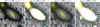 |
Fig. 1 Four RGB images of the DISK galaxy (ID = 1298 COSMOS, M* = 1.4 × 10¹⁰M⊙ at z = 0.15). The RGB channels correspond to the H, J, and I+V HST filters, respectively. Images were produced with the Gnuastro script astscript-color-faint-gray for q × s = 50 (first and second panels) and q × s = 400 (third and fourth panels), and for c = 1 (first and third panels) and c = 5 (second and fourth panels). Stamps have a field of view of 12 × 12 arcsec2 (200 × 200 px2). |
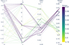 |
Fig. 2 Parallel coordinates plot for the 40 input configurations combining q × s (in log scale, first coordinate), c (second coordinate), standard deviation of the F1 score (third coordinate), and median values of the F1 score (fourth coordinate). Each configuration is color-coded according to the median F1 score. All the configurations with log(q × s) ≳ 1.7 (q × s ≥ 50) (independently of the contrast value, c) lead to the largest median values of the F1 score with the smallest values of the standard deviation of the F1 score. |
3.2.2 Averaged segmentation maps
We took advantage of the segmentations obtained with the different configurations to construct a robust segmentation mask and to quantify uncertain regions. We produced an averaged map with the 24 different configurations selected at the end of Sect. 3.2.1 and the three segmentation maps for each configuration that SAM infers. A total of 72 (24 × 3) segmentation maps were combined to obtain the average one. Segmentation maps are in a binary format: zeros for regions outside the truncation, and ones for regions inside it. Therefore, the averaged segmentation map ranges from 0 to 1 values per pixel: 0 means none of the segmentation maps include that pixel as part of the truncations; 1 means all the segmentation maps consider that pixel as part of the truncation; and intermediate values between 0 and 1 reflect different levels of agreement between the different segmentation maps for each configuration. By producing these averaged maps, we can determine whether the models converge on a similar solution for the truncation or not. For instance, images containing not only the central galaxy but other sources may lead to significantly different truncations for configurations with different q × s and c values. High contrast values could blend two distinct galaxies into one single object, producing different truncation masks, as is shown in Fig. 1. Contrarily, in some cases, large q × s and c values increase the contrast between the faint outskirts of a galaxy and its surrounding background, favoring a reliable determination of its truncation using SAM.
We defined the best truncation from the averaged segmented maps by applying a majority voting criteria. In other words, we computed the SAM truncation as the contour encompassing the regions with an averaged value above 0.5 (i.e., >50% of the segmentation maps agree). We also inferred the size of the truncation, denoted as R0.5, as the maximum distance from the galaxy’s center to the SAM truncation. Defining the size of the SAM truncation in this way allows us to reliably compare with the semi-major axis of the elliptical truncation presented in BT24, as is shown in Sect. 4.2. To estimate the robustness of the SAM predictions, we defined the relative error in the measurement of the size of the truncation following ∆R0.5 = (R0.5 − R0.7)/R0.5, where R0.7 is the size of the truncation enclosed by the contour at the 0.7 probability threshold. By definition, R0.7 ≤ R0.,5, and therefore ∆R0.5 ranges from 0 to 1 values. By looking at the values of ∆R0.5, we can easily determine whether the different contour levels in the averaged segmentation maps are in agreement or not, and therefore estimate the robustness of the truncations obtained. Large values of ∆R0.5 indicate that there is a significant difference in the measured size of the truncation (applying a majority voting criteria) and the area enclosed by a higher-probability (e.g., 0.7) contour level. This is mainly due to the presence of other sources (i.e., companions, artifacts, or star spikes) close to the truncation inferred by SAM. In summary, ∆R0.5 is certainly a way to determine whether the truncation and its size (R0.5) are affected by a contaminant that has been considered as part of the truncation inferred by SAM. Nevertheless, it will be possible to identify galaxies with close companions (and even mask them) from the source catalogs that will be published along with the Euclid images, and therefore exclude galaxies with less reliable SAM truncations and sizes in subsequent analysis.
In Fig. 3, we show the averaged segmentation maps for two example galaxies: DISK galaxy ID = 1298 in the COSMOS field (same as in Fig. 1) and ID = 6166 in the GOODSN field. Although ID = 1298 in the COSMOS is not a trivial case due to the presence of a bright companion galaxy in the top left corner of the image, by looking at the different metrics (e.g., F1 = 0.90), there is a good agreement between truncations derived by BT24 and the SAM truncation. The fraction of pixels (with respect to the total field of view) with low probability values (e.g., below 0.5, light gray pixels) in the averaged segmentation map is high, which indicates that some configurations of the input image include the neighbor galaxy as part of the truncation of the central galaxy. Nevertheless, the majority voting criteria does not include those regions within the truncation (i.e., the 0.5 contour level) favoring a high value of the Prec = 0.93. Moreover, a large fraction of the truncation derived by BT24 is also included in the SAM truncation, as is reflected by Rec = 0.88. In the case of ID = 6166 in the GOODSN field, there is a clear agreement between the different SAM predictions for the whole set of configurations. The majority of the predictions clearly depict the edge of the luminous matter in this particular galaxy, as is indicated by the low fraction of gray pixels (in fact, a majority of them are either black or white), and by the low value of R0.5 = 0.04. Besides, with F1 = 0.93, this is also an excellent example to illustrate the capacity of SAM to retrieve reliable galaxy truncations and sizes.
The choice of fixing a given probability threshold (e.g., 0.5 for the majority voting criteria) stems from the aim of this study: to develop a methodology for inferring stellar disk truncations in galaxy images in an automated and consistent manner. The 0.5 threshold was chosen as it balances precision and recall (see Sect. 4.1), providing robust segmentation maps while maintaining sensitivity to faint features in the galaxy outskirts. Alternative thresholds, such as 0.63, which maximizes the F1 score for our dataset, are explored in Sect. 4.1 to assess their impact on galaxy size measurements. While higher thresholds yield more conservative (i.e., purer) segmentations, they often exclude significant portions of the truncations (i.e., are less complete), particularly in galaxies with diffuse outer regions. Consequently, the 0.5 threshold was determined to be optimal for this study, ensuring a balance between capturing the full extent of the truncation and avoiding the inclusion of spurious features, both leading to a precise determination of the sizes of the galaxies in our dataset (see Sect. 4). Importantly, this threshold is not specifically tuned for this dataset but is instead a general and arbitrary choice, demonstrating its potential applicability to other datasets without requiring fine-tuning.
As we describe in Sect. 4.2, galaxies showing large values of ∆R0.5 would need to be inspected to check the validity of the sizes inferred or directly excluded from the analysis to avoid introducing inaccurate sizes. For those cases, defining the truncation as the contour encompassing the regions with an average value above 0.7 (or a different probability threshold) could lead to a better estimate of the truncation and its corresponding size with respect to BT24. For these reasons, we make publicly available the catalogs containing the parameters that characterize the truncations obtained with SAM and the averaged segmentation maps, allowing the user to use a different probability threshold.
 |
Fig. 3 SAM truncations for two example galaxies: ID = 1298 in the COSMOS field (left-hand panel) and ID = 6166 in the GOODSN field (right-hand panel). For each galaxy, we show an RGB image (left-hand panel) of the galaxy and the averaged segmentation map inferred with SAM (right-hand panel). The averaged segmentation map shows the SAM truncations (in gray) for different configurations of the input image, where darker regions indicate stronger agreement between different truncation estimates. The solid red contours depict the SAM truncation based on the majority voting criteria (above a 0.5 threshold), while the dashed red contours correspond to the regions above a 0.7 probability threshold. The blue ellipse corresponds to the truncation derived by BT24 parameterized by the semi-major axis (denoted as Redge) and the axis ratio, b/a (shown between brackets after the Redge value). We indicate in red the different metrics (F1, Rec, and Prec) when comparing the SAM and the BT24 truncation estimates, the size of the truncation (R0.5), and the relative error in the size of the truncation and the contour level at a 0.7 probability, denoted as ∆R0.5. |
4 Results
We aim to construct a model for determining stellar truncations in galaxy images, avoiding, to some extent, the need for specific preprocessing for each input image and survey. Additionally, this bypasses the necessity of relying on a particular dataset with derived truncations (such as BT24) for training, fine-tuning, or evaluating the SAM predictions for truncations. This is one of the advantages of using an AI foundational model like SAM. It should be noted that retrieving truncations using traditional methods, such as the approach presented in BT24, requires significant effort. In addition, masking secondary sources in the images, as a preliminary step before computing the surface brightness and color profiles, is partially manual work that demands considerable expertise.
Hereafter, the truncations presented in BT24 are only used for comparison in the following sections. The data supporting the findings of this study, including galaxy size measurements, averaged segmentation masks, and visualizations, are publicly available on GitHub6.
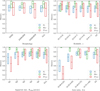 |
Fig. 4 From left to right, SAM’s performance as a function of: morphological type, redshift, apparent size (Redge , semi-major axis of the BT24 truncation) split in quintiles, and axis ratio of the BT24 truncation. Metrics are shown in different colors: F1 in blue, Rec in green, and Prec in red. Boxes represent the IQR, while the horizontal lines indicate the median value. F1 and Prec values decrease, while keeping high Rec values, for small and/or elongated galaxies. |
4.1 SAM performance in retrieving truncations
Beyond the results obtained for a particular galaxy, we computed the metrics introduced in Sect. 3.2 based on the truncations inferred with SAM and the estimates presented in BT24 for the whole dataset. In Fig. 4, we examine in detail these metrics as a function of the properties of the galaxies in the dataset: the apparent size of the BT24 truncation (Redge , in arcsec), the redshift (z), the axis ratio (b/a), and the morphology. Overall, we obtain F1 = 0.84, Prec = 0.84, and Rec = 0.92. This high value of Rec reflects the fact that SAM successfully recovers a large fraction of the pixels within the truncation of BT24. Besides, the lower Prec (equivalent to purity) compared to Rec (or completeness) indicates that SAM truncations extend beyond those derived by BT24. The harmonic mean of these two quantities, the F1 score, is still at an excellent level, despite SAM only being fed with RGB galaxy images and without the need for training nor fine-tuning the model (rather than surface brightness and mass profiles, and a labeled dataset, as done in BT24 and Fernández-Iglesias et al. 2024). Metrics are relatively constant, with median values above 0.8, independently of the galaxy morphology and redshift. However, F1 and Prec values drop for galaxies at the low end of the apparent size and axis ratio distributions. In both cases, Rec values are almost equal to 1 values, indicating that SAM tends to recover more extended truncations than BT24. Also, Rec values tend to decrease slightly toward the high end of the Redge distribution. Since cutouts have a fixed size, the smallest galaxies have a lower number of positive pixels. This means that a small number of FP can have a strong effect on the Prec. On the other hand, larger galaxies have a larger number of positive pixels, a factor on the denominator in the Prec definition, explaining the drop in this quantity with increasing size. Additionally, small and elongated galaxies are more affected by the PSF, which makes them look puffier and consequently leads SAM to infer slightly more extended truncations. This effect is more evident toward the minor axis of the truncation (see the two examples in Fig. A.1), and thus does not strongly affect the estimated size with SAM (R0.5).
To reinforce the choice of the 0.5 threshold in the majority voting criteria, we computed the threshold that maximises the F1 for our dataset when compared with BT24. We found the median value of this optimal threshold to be 0.63, which results in F1 = 0.84, Prec = 0.89, and Rec = 0.88. Differences in F1 with respect to the 0.5 threshold for the majority voting criteria are negligible (on the third decimal). However, increasing the threshold value from 0.5 to 0.63 improves the purity of the retrieved truncations (i.e., higher Prec) at the expense of reduced completeness (i.e., lower Rec). In practical terms, this means retrieving less extended truncations – and consequently smaller galaxy sizes – when using a higher threshold, which are not in the same level of agreement as those obtained with the 0.5 threshold in the majority voting criteria.
The 11 galaxies with the largest truncations according to BT24 in our dataset present truncations that extend beyond the image limits of 12 × 12 arcsec. These galaxies are not included in the analysis presented hereafter. In these cases, SAM has more difficulty accurately retrieving the stellar disk truncations because the galaxy cannot be completely shown in the image and there is not enough background field around the main galaxy for the model to contrast with. In fact, for six of these galaxies, SAM tends to underestimate the size of the truncations compared to BT24. To avoid this, it would be necessary to produce larger images for the more extended galaxies and check if the truncations are better identified compared to the standard image sizes used for the whole dataset. While SAM can easily handle varying sizes and aspects of input images (i.e., they do not need to be of a fixed size), this is beyond the scope of the current study. We shall consider producing images with a field of view that better accommodates the apparent size of the galaxy when applying this methodology to real Euclid data in the future.
4.2 Galaxy sizes inferred from SAM truncations
As is described in Sect. 3.2, we estimated the size of the galaxy, denoted as R0.5, as the maximum distance from the center of the galaxy to the SAM truncation from the majority voting criteria. This choice of galaxy size, measured in the averaged segmentation maps, was made to facilitate a comparison with the size derived by BT24 as the semi-major axis of the elliptical truncation. We derived the relative error at measuring galactic sizes between the SAM predictions (R0.5) and the BT24 estimates (i.e., the semi-major axis of the elliptical truncation, Redge), as follows: (R0.5 − Redge)/Redge. In Fig. 5, we show the relative error in the size estimates as a function of different galaxy parameters. We find median size values inferred with SAM to be overestimated with respect to BT24, independently of the morphological type, although the median relative error is always <5%. There is not a clear dependence on redshift, although the median values of the size relative error are below the 8% for all the redshift bins analyzed. The largest discrepancies (relative errors between 12 and 14%) are due to galaxies with the smallest apparent sizes (i.e., those within Q1 of the distribution), and the most elongated galaxies (i.e., b/a ≲ 0.25), the sizes of which SAM tends to overestimate with respect to BT24.
Using the definition of the relative error in the measurement of the size of the SAM truncation described in Sect. 3.2, denoted as ΔR0.5, we examined the robustness and reliability of the galactic sizes inferred with SAM. In Fig. 6, we show the distribution of the relative error on the size of the truncation inferred with SAM with respect to the BT24 measurements, denoted as (R0.5 − Redge)/Redge, as a function of ΔR0.5. The median values of (R0.5 − Redge)/Redge are constrained within less than ~0.05 and the interquartile range (IQR) is below ~0.10 for the Q1-Q4 quintiles. For the largest values of the ΔR0.5 distribution (the Q5 quintile), median relative errors exceed the ~0.10 level. Besides, the most extreme values of (R0.5 − Redge)/Redge correspond to those cases with ΔR0.5 in the Q5 quintile, as is shown by the length of the whiskers. Therefore, it is possible to identify cases with large relative errors in the sizes derived with SAM and with respect to BT24 estimates by selecting those with large ΔR0.5 values, without depending on the truncations and sizes derived by BT24. We illustrate this in Fig. A.2, in which we show the SAM truncations for two galaxies with ΔR0.5 in the Q5 quintile.
Overall, in Fig. 7, we find a relative error for the size of the galaxy of  for the whole dataset, expressed as the median value and the IQR of the distribution. Then, we excluded from this analysis galaxies for which the sizes derived with SAM are less reliable: ΔR0.5 ≳ 0.17 (those within the Q5 quintile, see Fig. 6) and elongated in projection with b/a < 0.25 (those within the Q1 quintile, see the bottom right panel in Fig. 5). It is clear how this selection mostly excludes cases at the high end of the (R0.5 − Redge)/Redge distribution, which leads to a slightly better average size estimate,
  . In Fig. A.3, we show two examples of galaxies within the high end of the (R0.5 − Redge)/Redge distribution, even though they fall within the Q1-Q4 quintiles of the ΔR0.5 distribution. However, it will be possible to identify galaxies with close companions, which are likely to have less reliable SAM truncations and sizes, using the source catalogs that will be published along with the Euclid images.
This excellent result demonstrates the enormous potential of using SAM to retrieve galaxy sizes in large datasets such as the Euclid Wide Survey in an automated way, without the need to train the model or heavily preprocess the input images. Moreover, as can be seen in the right-hand panel in Fig. A.3, SAM can help retrieve truncations more accurately in nonsymmetric galaxies that could be problematic for other approaches that rely on the assumption of elliptical symmetry for the truncations.
5 Conclusions
In this study, we explore the potential of using an AI foundational model, specifically SAM, to retrieve galactic sizes in upcoming Euclid data from the stellar disk truncation. Our findings suggest that SAM can significantly optimize and accelerate the process of galactic size measurement in an automated manner. Although our current results are not yet competitive with those achieved by supervised models (e.g., Fernández-Iglesias et al. 2024 obtained an F1 = 0.91), SAM eliminates the need for extensive training or fine-tuning typically required by these models, achieving a significantly high performance. Furthermore, without relying on any physical assumptions about the shape of the truncation, SAM can retrieve reliable truncations and sizes for nonsymmetric galaxies – cases that can be problematic when addressed by other approaches.
SAM’s segmentation tasks were conducted on a system with an NVIDIA RTX A5000 GPU (24 GB RAM) and an AMD Ryzen 9 5900X 12-Core Processor. With this setup, SAM can infer galaxy sizes with an error of ≈3% error (an error of ≈1% if unreliable measurements are excluded) with respect to BT24, with an average runtime of approximately 1 minute per galaxy (i.e., roughly 2 seconds per configuration), considering all 24 different configurations per galaxy described in Sect. 3.2.1. While GPU acceleration significantly reduced processing time, SAM can also operate on CPU systems, albeit with slower runtimes. The model’s scalability is advantageous for processing large datasets like the Euclid Wide Survey, for which segmentation tasks could be parallelized across multiple GPUs or computational nodes.
Still, the entire process could be optimized further; for instance, by reducing the number of pixels (e.g., through rebinning) and the number of input configurations per galaxy. Moreover, different observational scenarios (e.g., less massive or LSB galaxies) from those described in this study might require additional tuning during the preprocessing of input images. For example, for galaxies with LSB or at higher redshifts than those in our dataset (where surface brightness dimming is significant), increasing the product q × s and the contrast (c) in the preprocessing stage can enhance the visibility of faint outer regions, leading to improved segmentation accuracy. Different optimizations will be explored when applying this methodology to the upcoming Euclid data, ensuring the robustness and scalability of SAM for larger and more diverse datasets.
Using the optimal input configurations presented in Sect. 3.2.1, we have demonstrated an excellent performance in retrieving stellar disk truncations and galaxy sizes for the galaxies in our dataset (as is shown in Sect. 4). It is worth noting that our dataset already encompasses a broad variety of sources in terms of galaxy sizes, axis ratios, and redshift coverage (up to z ~ 1). However, future applications of SAM to datasets of galaxies with significantly different properties, such as non-disk-like galaxies, may benefit from systematic parameter optimization.
Nonetheless, the results presented in this manuscript may serve as a proof of concept and represent a substantial advancement in the field, allowing researchers to bypass the time-consuming stages and human supervision required by other traditional methods, such as those described in Chamba et al. (2022) and Buitrago & Trujillo (2024).
During the preparation of this manuscript, the Meta AI7 team published an updated model for segmentation tasks, SAM 2 (Ravi et al. 2024). SAM 2 extends the previous version by performing visual segmentation in videos. We applied the whole pipeline described in this manuscript using SAM 2 over our dataset to retrieve stellar disk truncations and galactic sizes in the same way as was done for SAM. Surprisingly, the results obtained with SAM 2 are not as satisfactory as those retrieved with SAM. After a closer examination of the results, we detect that SAM 2 tends to segment more frequently the inner parts of the galaxies in the dataset. This leads to a better purity (Prec = 0.90) but worse completeness (Rec = 0.88), although showing a similar median, F1 = 0.84. Consequently, the majority voting criteria applied to SAM 2 averaged segmentation maps tend to underestimate the size of the galaxies in our dataset compared to BT24. Although with a different configuration SAM 2 could also be a valid approach to infer galaxy truncations and sizes, we leave these tasks for future work and rely on the excellent results provided by SAM and described throughout this study.
By leveraging SAM, we can achieve rapid and reliable galactic size estimations, which is crucial for large-scale astronomical surveys like the Euclid Wide Survey. The integration of foundational AI models like SAM into astronomical data analysis holds great promise. In particular, SAM will allow us to estimate truncations for millions of galaxies up to z ~ 2 when applied to the upcoming Euclid Wide Survey, paving the way for understanding the physical processes that shape galaxy evolution across cosmic time. Accurate galaxy size measurements derived from stellar disk truncations are critical for refining the mass-size relation, a fundamental aspect of understanding galaxy evolution. These measurements can also inform studies of galaxy morphology and star formation mechanisms, providing an insight into how galaxies evolve in different cosmic environments. Within the context of Euclid, precise size estimates will contribute to mapping the distribution of galaxies across large-scale structures and understanding the interplay between galaxy evolution and dark matter halos, key to Euclid’s cosmological goals.
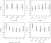 |
Fig. 5 From left to right, relative difference between the size of the galaxy measured from the SAM truncation (denoted as R0.5) and the semi-major axis of the truncation ellipse in BT24 (denoted as Redge) as a function of: morphological type, redshift, apparent size (Redge , semi-major axis of the BT24 truncation) split in quintiles, and axis ratio of the BT24 truncation. Boxes represent the IQR, while the horizontal lines indicate the median value. SAM truncations are on average overestimated with respect to BT24 truncations for the most elongated (in projection) and/or for the (apparently) smallest galaxies. |
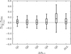 |
Fig. 6 Relative error on the size of the truncation inferred with SAM with respect to the BT24 measurements as a function of the relative error on the size of the truncation derived from the averaged SAM segmentation maps (ΔR0.5) split in quintiles. Boxes represent the IQR and whiskers extend from the box to the farthest data point lying within 1.5 × IQR from the box, while the horizontal lines indicate the median value. Median values (and the scatter) of the relative error on the size obtained with SAM compared to BT24 are below the ~5% level for all quintiles with the exception of Q5. For Q5, where the differences between the size of the truncation at 0.5 and 0.7 probability thresholds are the largest, the median value of the relative error on the size of the truncation inferred with SAM surpasses the ~10% level, with a clear increase in the scatter. |
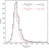 |
Fig. 7 Distributions of the relative error between the size of the galaxy measured from the SAM truncation (denoted as R0.5) and the semimajor axis of the truncation ellipse in BT24 (denoted as Redge). The solid black histogram corresponds to the whole sample of 1047 galaxies, while the dashed red histogram shows the distribution for 774 galaxies with ΔR0.5 ≲ 0.17 (i.e., excluding those within the Q5 quintile) and b/a > 0.25. The median and IQR of the relative error between the two estimates for both distributions are also shown. |
Acknowledgements
J.V-.F. acknowledges Raúl Infante-Sainz and Mohammad Akhlaghi for their insightful comments, and advice, which significantly contributed to the development of this work. J.V-.F., F.B., J.F-.I. and S.R. acknowledge support from the project the GEELSBE project with reference PID2020-116188GA-I00, funded by MICIU/AEI /10.13039/501100011033. J.V-.F., F.B., J.F-.I., S.R., B.S. and H.D.S. also acknowledge support from the GEELSBE2 project with reference PID2023-150393NB-I00 funded by MCIU/AEI/10.13039/501100011033 and the FSE+. J.V-.F. and H.D.S. acknowledge the financial support from the European Union - NextGenerationEU and the Spanish Ministry of Science and Innovation through the Recovery and Resilience Facility project ICTS-MRR-2021-03-CEFCA and the support from the grant PID2022-138896NA-C54. H.D.S. acknowledges financial support by RyC2022- 030469-I grant, funded by MCIN/AEI/10.13039/501100011033 and FSE+. This work has made use of the Rainbow Cosmological Surveys Database, which is operated by the Centro de Astrobiología (CAB/INTA), partnered with the University of California Observatories at Santa Cruz (UCO/Lick,UCSC). Based on zCOSMOS observations carried out using the Very Large Telescope at the ESO Paranal Observatory under Programme ID: LP175.A0839. We have used extensively the following software packages: MATPLOTLIB (Hunter 2007), PYTORCH (Paszke et al. 2019), and Segment Anything Model (Kirillov et al. 2023).
Appendix A Examples of galaxy truncations derived with SAM
In this appendix we show a selection of galaxy images to illustrate the potential of SAM to derive stellar disk truncations in ‘euclidized’ galaxy images. All the images shown in this section are produced with the Gnuastro script astscript-color-faint-gray for q × s = 100 and c = 1.
In Fig. A.1, we show two galaxies with extremely elongated shapes, i.e., b/a < 0.25, for which the Prec and F1 tend to be worse than for more rounded galaxies, as shown in Fig. 4. The example in the left panel (19670 COSMOS) shows a galaxy with b/a = 0.2 and close to the high-end of the redshift distribution (z = 0.91). Although the central galaxy is close to another galaxy with apparently similar brightness, the SAM truncation and its estimated size are in good agreement with the findings of BT24. Nevertheless, we find a F1 = 0.76 because of the SAM truncation extends beyond the BT24 truncation (Prec = 0.63). The relative error in the size with respect to BT24 is (R0.5 − Redge)/Redge ≈ 0.05. The galaxy in the right panel (22430 UDS) has a b/a = 0.2 at a z = 0.53 and, therefore, with a larger apparent size compared to the previous example. The SAM truncation is in excellent agreement with the findings by BT24, showing a F1 = 0.92 and a relative error in the size of (R0.5 − Redge)/Redge ≈ 0.06. In both cases, the different estimates of the truncation are in good agreement for the different input configurations, as the low values of ΔR0.5 = 0.01 reflect.
Examples of galaxy images, 5556 GOODSS and 8203 EGS, with large values of ΔR0.5 ≳ 0.17 (within the Q5 quintile, see Fig. 6) are shown in Fig. A.2. In both cases, the large values of ΔR0.5 are due to the presence of a neighbor galaxy close to the central galaxy. While the SAM truncation at a 0.5 probability threshold includes the close galaxy within the truncation, the contour at a 0.7 probability threshold leads to a better estimate of the truncation and its size. In these cases, it is possible to correct the size of the SAM truncation by the factor ΔR0.5 to better agree with the results obtained by BT24. By doing so, also the metrics shown in the figure would increase.
In Fig. A.3, we show two examples of galaxies, 11170 COSMOS and 19000 COSMOS, for which the size estimate with SAM of more than 20% larger than the size measured by BT24, even though they both exhibit small values of ΔR0.5 = 0.02. These cases correspond to galaxies at the high-end of the (R0.5 − Redge)/Redge distribution shown in Fig. 7 when ΔR0.5 ≳ 0.17 are not included, and for which neither the truncation defined at 0.5 or 0.7 probability thresholds lead to a good estimate of the truncation and its size. Therefore, to obtain a better estimate of the size of the truncation for 11170 COSMOS with respect to BT24, the truncation should be derived for an even higher probability threshold. For 19000 COSMOS, the difference between R0.5 and Redge is due to a bright extension of the galaxy toward the bottom-right corner of the figure. This structure, likely a tidal feature produced by a past interaction of the central galaxy with another galaxy, seems to be part of the central galaxy. Therefore, the measured size of the truncation with SAM might not be as inaccurate as it is when compared with the truncation derived by BT24.
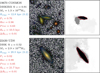 |
Fig. A.1 Galaxy images with elongated shapes (b/a < 0.25). Image details are described in the caption of Fig. 3. |
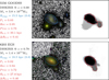 |
Fig. A.2 Galaxy images with ΔR0.5 ≳ 0.17 (within the Q5 quintile). Image details are described in the caption of Fig. 3. |
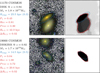 |
Fig. A.3 Galaxy images with ΔR0.5 ≲ 0.17 (within the Q1-Q4 quintile) and (R0.5 − Red𝑔e)/Red𝑔e > 0.20. Image details are described in the caption of Fig. 3. |
References
- Barro, G., Pérez-González, P. G., Cava, A., et al. 2019, ApJS, 243, 22 [NASA ADS] [CrossRef] [Google Scholar]
- Bommasani, R., Hudson, D. A., Adeli, E., et al. 2021, arXiv e-prints [arXiv:2108.07258] [Google Scholar]
- Boucaud, A., Huertas-Company, M., Heneka, C., et al. 2020, MNRAS, 491, 2481 [Google Scholar]
- Bretonnière, H., Boucaud, A., & Huertas-Company, M. 2021, arXiv e-prints [arXiv:2111.15455] [Google Scholar]
- Buitrago, F., & Trujillo, I. 2024, A&A, 682, A110 [NASA ADS] [CrossRef] [EDP Sciences] [Google Scholar]
- Burke, C. J., Aleo, P. D., Chen, Y.-C., et al. 2019, MNRAS, 490, 3952 [NASA ADS] [CrossRef] [Google Scholar]
- Chabrier, G. 2003, PASP, 115, 763 [Google Scholar]
- Chamba, N. 2020, Res. Notes Am. Astron. Soc., 4, 117 [NASA ADS] [Google Scholar]
- Chamba, N., Trujillo, I., & Knapen, J. H. 2022, A&A, 667, A87 [NASA ADS] [CrossRef] [EDP Sciences] [Google Scholar]
- Damjanov, I., Zahid, H. J., Geller, M. J., et al. 2019, ApJ, 872, 91 [NASA ADS] [CrossRef] [Google Scholar]
- Díaz-García, S., Comerón, S., Courteau, S., et al. 2022, A&A, 667, A109 [NASA ADS] [CrossRef] [EDP Sciences] [Google Scholar]
- Dieleman, S., Willett, K. W., & Dambre, J. 2015, MNRAS, 450, 1441 [NASA ADS] [CrossRef] [Google Scholar]
- Domínguez Sánchez, H., Huertas-Company, M., Bernardi, M., Tuccillo, D., & Fischer, J. L. 2018, MNRAS, 476, 3661 [Google Scholar]
- Duc, P.-A., Cuillandre, J.-C., Karabal, E., et al. 2015, MNRAS, 446, 120 [Google Scholar]
- Euclid Collaboration (Borlaff, A. S., et al.) 2022, A&A, 657, A92 [NASA ADS] [CrossRef] [EDP Sciences] [Google Scholar]
- Farias, H., Ortiz, D., Damke, G., Jaque Arancibia, M., & Solar, M. 2020, Astron. Comput., 33, 100420 [NASA ADS] [CrossRef] [Google Scholar]
- Fernández-Iglesias, J., Buitrago, F., & Sahelices, B. 2024, A&A, 683, A145 [NASA ADS] [CrossRef] [EDP Sciences] [Google Scholar]
- González, R. E., Muñoz, R. P., & Hernández, C. A. 2018, Astron. Comput., 25, 103 [CrossRef] [Google Scholar]
- Grogin, N. A., Kocevski, D. D., Faber, S. M., et al. 2011, ApJS, 197, 35 [NASA ADS] [CrossRef] [Google Scholar]
- Hausen, R., & Robertson, B. E. 2020, ApJS, 248, 20 [CrossRef] [Google Scholar]
- Huertas-Company, M., Gravet, R., Cabrera-Vives, G., et al. 2015, ApJS, 221, 8 [NASA ADS] [CrossRef] [Google Scholar]
- Hunter, J. D. 2007, Comput. Sci. Eng., 9, 90 [NASA ADS] [CrossRef] [Google Scholar]
- Illingworth, G., Magee, D., Bouwens, R., et al. 2016, arXiv e-prints [arXiv:1606.00841] [Google Scholar]
- Infante-Sainz, R., & Akhlaghi, M. 2024, Res. Notes Am. Astron. Soc., 8, 10 [Google Scholar]
- Kirillov, A., Mintun, E., Ravi, N., et al. 2023, arXiv e-prints [arXiv:2304.02643] [Google Scholar]
- Koekemoer, A. M., Faber, S. M., Ferguson, H. C., et al. 2011, ApJS, 197, 36 [NASA ADS] [CrossRef] [Google Scholar]
- Lilly, S. J., Le Brun, V., Maier, C., et al. 2009, ApJS, 184, 218 [Google Scholar]
- Lupton, R., Blanton, M. R., Fekete, G., et al. 2004, PASP, 116, 133 [NASA ADS] [CrossRef] [Google Scholar]
- Martín-Navarro, I., Bakos, J., Trujillo, I., et al. 2012, MNRAS, 427, 1102 [Google Scholar]
- Martín-Navarro, I., Trujillo, I., Knapen, J. H., Bakos, J., & Fliri, J. 2014, MNRAS, 441, 2809 [CrossRef] [Google Scholar]
- Martínez-Lombilla, C., Trujillo, I., & Knapen, J. H. 2019, MNRAS, 483, 664 [CrossRef] [Google Scholar]
- Mihos, J. C. 2019, arXiv e-prints [arXiv:1909.09456] [Google Scholar]
- Nayyeri, H., Hemmati, S., Mobasher, B., et al. 2017, ApJS, 228, 7 [NASA ADS] [CrossRef] [Google Scholar]
- Paillassa, M., Bertin, E., & Bouy, H. 2020, A&A, 634, A48 [NASA ADS] [CrossRef] [EDP Sciences] [Google Scholar]
- Parker, L., Lanusse, F., Golkar, S., et al. 2024, MNRAS, 531, 4990 [Google Scholar]
- Paszke, A., Gross, S., Massa, F., et al. 2019, in Advances in Neural Information Processing Systems, eds. H. Wallach, H. Larochelle, A. Beygelzimer, et al. (Newry, UK: Curran Associates, Inc.), 32 [Google Scholar]
- Ravi, N., Gabeur, V., Hu, Y.-T., et al. 2024, arXiv e-prints [arXiv:2408.00714] [Google Scholar]
- Santini, P., Ferguson, H. C., Fontana, A., et al. 2015, ApJ, 801, 97 [Google Scholar]
- Schaye, J. 2004, ApJ, 609, 667 [NASA ADS] [CrossRef] [Google Scholar]
- Sersic, J. L. 1968, Atlas de Galaxias Australes (Cordoba, Argentina: Observatorio Astronomico) [Google Scholar]
- Stefanon, M., Yan, H., Mobasher, B., et al. 2017, ApJS, 229, 32 [NASA ADS] [CrossRef] [Google Scholar]
- Straatman, C. M. S., van der Wel, A., Bezanson, R., et al. 2018, ApJS, 239, 27 [NASA ADS] [CrossRef] [Google Scholar]
- Tanoglidis, D., & Jain, B. 2024, Res. Notes Am. Astron. Soc., 8, 265 [Google Scholar]
- Tanoglidis, D., Ciprijanović, A., Drlica-Wagner, A., et al. 2022, Astron. Comput., 39, 100580 [NASA ADS] [CrossRef] [Google Scholar]
- Trujillo, I., & Fliri, J. 2016, ApJ, 823, 123 [Google Scholar]
- Trujillo, I., Chamba, N., & Knapen, J. H. 2020, MNRAS, 493, 87 [NASA ADS] [CrossRef] [Google Scholar]
- van der Kruit, P. C. 1979, A&AS, 38, 15 [NASA ADS] [Google Scholar]
- van der Kruit, P. C., & Searle, L. 1981a, A&A, 95, 105 [NASA ADS] [Google Scholar]
- van der Kruit, P. C., & Searle, L. 1981b, A&A, 95, 116 [NASA ADS] [Google Scholar]
- van der Wel, A., Noeske, K., Bezanson, R., et al. 2016, ApJS, 223, 29 [Google Scholar]
- van der Wel, A., Bezanson, R., D’Eugenio, F., et al. 2021, ApJS, 256, 44 [NASA ADS] [CrossRef] [Google Scholar]
- Vega-Ferrero, J., Domínguez Sánchez, H., Bernardi, M., et al. 2021, MNRAS, 506, 1927 [NASA ADS] [CrossRef] [Google Scholar]
- Vega-Ferrero, J., Huertas-Company, M., Costantin, L., et al. 2024, ApJ, 961, 51 [NASA ADS] [CrossRef] [Google Scholar]
- Walmsley, M., Smith, L., Lintott, C., et al. 2020, MNRAS, 491, 1554 [Google Scholar]
- Walmsley, M., Lintott, C., Géron, T., et al. 2022, MNRAS, 509, 3966 [Google Scholar]
- Zhang, C., Liu, L., Cui, Y., et al. 2023, arXiv e-prints [arXiv:2305.08196] [Google Scholar]
All Figures
|
Fig. 1 Four RGB images of the DISK galaxy (ID = 1298 COSMOS, M* = 1.4 × 10¹⁰M⊙ at z = 0.15). The RGB channels correspond to the H, J, and I+V HST filters, respectively. Images were produced with the Gnuastro script astscript-color-faint-gray for q × s = 50 (first and second panels) and q × s = 400 (third and fourth panels), and for c = 1 (first and third panels) and c = 5 (second and fourth panels). Stamps have a field of view of 12 × 12 arcsec2 (200 × 200 px2). |
| In the text | |
|
Fig. 2 Parallel coordinates plot for the 40 input configurations combining q × s (in log scale, first coordinate), c (second coordinate), standard deviation of the F1 score (third coordinate), and median values of the F1 score (fourth coordinate). Each configuration is color-coded according to the median F1 score. All the configurations with log(q × s) ≳ 1.7 (q × s ≥ 50) (independently of the contrast value, c) lead to the largest median values of the F1 score with the smallest values of the standard deviation of the F1 score. |
| In the text | |
|
Fig. 3 SAM truncations for two example galaxies: ID = 1298 in the COSMOS field (left-hand panel) and ID = 6166 in the GOODSN field (right-hand panel). For each galaxy, we show an RGB image (left-hand panel) of the galaxy and the averaged segmentation map inferred with SAM (right-hand panel). The averaged segmentation map shows the SAM truncations (in gray) for different configurations of the input image, where darker regions indicate stronger agreement between different truncation estimates. The solid red contours depict the SAM truncation based on the majority voting criteria (above a 0.5 threshold), while the dashed red contours correspond to the regions above a 0.7 probability threshold. The blue ellipse corresponds to the truncation derived by BT24 parameterized by the semi-major axis (denoted as Redge) and the axis ratio, b/a (shown between brackets after the Redge value). We indicate in red the different metrics (F1, Rec, and Prec) when comparing the SAM and the BT24 truncation estimates, the size of the truncation (R0.5), and the relative error in the size of the truncation and the contour level at a 0.7 probability, denoted as ∆R0.5. |
| In the text | |
|
Fig. 4 From left to right, SAM’s performance as a function of: morphological type, redshift, apparent size (Redge , semi-major axis of the BT24 truncation) split in quintiles, and axis ratio of the BT24 truncation. Metrics are shown in different colors: F1 in blue, Rec in green, and Prec in red. Boxes represent the IQR, while the horizontal lines indicate the median value. F1 and Prec values decrease, while keeping high Rec values, for small and/or elongated galaxies. |
| In the text | |
|
Fig. 5 From left to right, relative difference between the size of the galaxy measured from the SAM truncation (denoted as R0.5) and the semi-major axis of the truncation ellipse in BT24 (denoted as Redge) as a function of: morphological type, redshift, apparent size (Redge , semi-major axis of the BT24 truncation) split in quintiles, and axis ratio of the BT24 truncation. Boxes represent the IQR, while the horizontal lines indicate the median value. SAM truncations are on average overestimated with respect to BT24 truncations for the most elongated (in projection) and/or for the (apparently) smallest galaxies. |
| In the text | |
|
Fig. 6 Relative error on the size of the truncation inferred with SAM with respect to the BT24 measurements as a function of the relative error on the size of the truncation derived from the averaged SAM segmentation maps (ΔR0.5) split in quintiles. Boxes represent the IQR and whiskers extend from the box to the farthest data point lying within 1.5 × IQR from the box, while the horizontal lines indicate the median value. Median values (and the scatter) of the relative error on the size obtained with SAM compared to BT24 are below the ~5% level for all quintiles with the exception of Q5. For Q5, where the differences between the size of the truncation at 0.5 and 0.7 probability thresholds are the largest, the median value of the relative error on the size of the truncation inferred with SAM surpasses the ~10% level, with a clear increase in the scatter. |
| In the text | |
|
Fig. 7 Distributions of the relative error between the size of the galaxy measured from the SAM truncation (denoted as R0.5) and the semimajor axis of the truncation ellipse in BT24 (denoted as Redge). The solid black histogram corresponds to the whole sample of 1047 galaxies, while the dashed red histogram shows the distribution for 774 galaxies with ΔR0.5 ≲ 0.17 (i.e., excluding those within the Q5 quintile) and b/a > 0.25. The median and IQR of the relative error between the two estimates for both distributions are also shown. |
| In the text | |
|
Fig. A.1 Galaxy images with elongated shapes (b/a < 0.25). Image details are described in the caption of Fig. 3. |
| In the text | |
|
Fig. A.2 Galaxy images with ΔR0.5 ≳ 0.17 (within the Q5 quintile). Image details are described in the caption of Fig. 3. |
| In the text | |
|
Fig. A.3 Galaxy images with ΔR0.5 ≲ 0.17 (within the Q1-Q4 quintile) and (R0.5 − Red𝑔e)/Red𝑔e > 0.20. Image details are described in the caption of Fig. 3. |
| In the text | |
Current usage metrics show cumulative count of Article Views (full-text article views including HTML views, PDF and ePub downloads, according to the available data) and Abstracts Views on Vision4Press platform.
Data correspond to usage on the plateform after 2015. The current usage metrics is available 48-96 hours after online publication and is updated daily on week days.
Initial download of the metrics may take a while.