| Issue |
A&A
Volume 693, January 2025
|
|
|---|---|---|
| Article Number | A184 | |
| Number of page(s) | 23 | |
| Section | Stellar structure and evolution | |
| DOI | https://doi.org/10.1051/0004-6361/202451995 | |
| Published online | 15 January 2025 | |
KIC 4150611: A quadruply eclipsing heptuple star system with a g-mode period-spacing pattern
Asteroseismic modelling of the g-mode period-spacing pattern
1
Institute of Astronomy (IvS), KU Leuven, Celestijnenlaan 200D, 3001 Leuven, Belgium
2
IRAP, Université de Toulouse, CNRS, UPS, CNES, 14 Avenue Édouard Belin, 31400 Toulouse, France
3
Department of Astrophysics, IMAPP, Radboud University Nijmegen, PO Box 9010, 6500 GL Nijmegen, The Netherlands
4
Max Planck Institute for Astronomy, Koenigstuhl 17, 69117 Heidelberg, Germany
⋆ Corresponding author; This email address is being protected from spambots. You need JavaScript enabled to view it.
Received:
26
August
2024
Accepted:
25
November
2024
Abstract
Context. KIC 4150611 is a high-order (seventh-order) multiple composed of a triple system with: a F1V primary (Aa), which is eclipsed on a 94.2 d period by a tight binary composed of two K/M dwarfs (Ab1 and Ab2) that also eclipse each other; an eccentric, eclipsing binary composed of two G stars (Ba and Bb); and another faint eclipsing binary composed of two stars of unknown spectral type (Ca and Cb). In addition to its many eclipses, the system is an triple-lined spectroscopic multiple (Aa, Ba, and Bb) and the primary (Aa) is a hybrid pulsator that exhibits high amplitude pressure and gravity modes (g-modes). Furthermore, its g-modes are arrayed in a period-spacing pattern, which greatly assists with mode identification and asteroseismic modelling. In aggregate, this richness in physics offers an excellent opportunity to obtain a precise physical characterisation for some of the stars in this system.
Aims. In this work we estimate the stellar parameters of the primary (Aa) by performing asteroseismic analysis on its period-spacing pattern.
Methods. We used the C-3PO neural network to perform asteroseismic modelling of the g-mode period-spacing pattern of Aa, examining the interplay of this information with external constraints from spectroscopy (Teff and log(g)) and eclipse modelling (R). To estimate the level of uncertainty due to different frequency extraction and pattern identification processes, we considered four different variations of the period-spacing patterns. To better understand the correlations between and the uncertainty structure of our parameter estimates, we also employed a classical, parameter-based Markov chain Monte Carlo (MCMC) grid search on four different stellar grids.
Results. The externally constrained model that best fits the period-spacing pattern arrives at estimates of the stellar properties for Aa of M = 1.51 ± 0.05 M⊙, Xc = 0.43 ± 0.04, R = 1.66 ± 0.1 R⊙, fov = 0.010, Ωc = 1.58 ± 0.01 d−1 with rigid rotation to within the measurement errors, log(Teff) = 3.856 ± 0.008 dex, log(g) = 4.18 ± 0.04 dex, and log(L) = 0.809 ± 0.005 dex, which agree well with previous measurements from eclipse modelling, spectroscopy, and the Gaia DR3 luminosity.
Conclusions. We find that the near-core properties of the best-fitting asteroseismic models are consistent with external constraints from eclipse modelling and spectroscopy. For stellar properties not related to the near-core region, external constraints on the asteroseismic best-fitting models are informative. Aa appears to be a typical example of a γ Dor star, fitting well within existing populations. We find that Aa is quasi-rigidly rotating to within the uncertainties, and note that the asteroseismic age estimate for Aa (1100 ± 100 Myr) is considerably older than the young age (35 Myr) implied by previous isochrone fits to the B binary in the literature. Our MCMC parameter-based grid search agrees well with our pattern-modelling approach. Improved future modelling could come from detailed coverage of metallicity effects and a careful treatment of envelope physics.
Key words: asteroseismology / binaries: eclipsing / binaries: spectroscopic / stars: oscillations
© The Authors 2025
 Open Access article, published by EDP Sciences, under the terms of the Creative Commons Attribution License (https://creativecommons.org/licenses/by/4.0), which permits unrestricted use, distribution, and reproduction in any medium, provided the original work is properly cited.
This article is published in open access under the Subscribe to Open model. This email address is being protected from spambots. You need JavaScript enabled to view it. to support open access publication.
1. Introduction
Asteroseismology, the study of stellar oscillations, stands as a cornerstone in modern astrophysics, offering unique insights into fundamental stellar properties. The sensitivity of stellar oscillation frequencies to the interior structure has opened the door to the measurement of stellar properties that are beyond the reach of surface observations. We can exploit this direct link between theoretical models and observations to refine our understanding of stellar evolution (Aerts 2021).
Asteroseismology’s role in modern astrophysics has grown rapidly since the advent of space-based planet-hunting surveys such as CoRoT (Baglin 2003), Kepler (Borucki et al. 2010), and TESS (Ricker et al. 2015), which provided near-uninterrupted, high-precision photometry with regular cadence on long time bases. One outcome of this new era of space-based photometry has been the detection of low-frequency gravity modes (g-modes) in large numbers of stars (Van Reeth et al. 2015a,b; Li et al. 2019a,b). This had previously been impossible due to the logistical challenges of obtaining long time base data for even a small number of stars (e.g. De Cat & Aerts 2002; Aerts et al. 2004; De Cat et al. 2006). Gravity-mode oscillations are waves that propagate with buoyancy as the dominant restoring force, and are particularly sensitive to the near-core stellar properties (Miglio et al. 2008). Pressure modes (p-modes) have pressure as their dominant restoring force and have higher frequencies. These modes are more sensitive to bulk stellar properties such as the average stellar density and envelope properties such as rotation (Aerts et al. 2010).
In order for stellar oscillations to be observed, they must propagate to the surface, where they produce variations in the stellar flux. Main sequence stars more massive than approximately 1.2 M⊙ have a convective core and a radiative envelope. As g-modes are restored by buoyancy, they can propagate through the radiative envelope from the near-core region to the surface, where they are observed, but not within the convective stellar core.
Stars with masses between approximately 1.4 M⊙ and 1.9 M⊙ with observed g-mode pulsations are known as γ Doradus (γ Dor) pulsators and feature g-mode pulsations excited via convective flux blocking (Dupret et al. 2005). Some γ Dor stars have overlap with the δ Scuti (δ Sct) stars, which typically have masses between 1.5 and 2.5 M⊙ and exhibit p-mode oscillations driven by the opacity-driven heat engine mechanism.
The primary component of KIC 41506111 is an example of a γ Dor–δ Sct hybrid pulsator: a star that exhibits both δ Sct and γ Dor pulsations (Uytterhoeven et al. 2011). In this work we focus on modelling the g-mode period-spacing pattern. The prominent p-mode pulsations do not form a part of this analysis, as without mode identification they provide a negligible constraining power – but add significant modelling complexity – to the analysis. Analysis of the p-mode δ Sct pulsations can be found in Shibahashi & Kurtz (2012) and Balona (2014).
KIC 4150611 is a high-order (seventh-order) multiple star system with four different sets of eclipses. The primary, Aa, is a bright (V ≈ 8 mag) F1V-type star that is in an eclipsing 94.2 d circular orbit with a 1.52 d self-eclipsing binary (Ab) composed of two dim (negligible light contribution) K/M dwarf stars (Ab1 and Ab2). The resulting primary eclipses of the triple geometry are complicated, varying significantly between eclipses depending on the phase of the Ab binary. Associated on roughly a 1000 yr orbit with the A triple is the eccentric 8.65 d eclipsing B binary, composed of two near-identical G-type stars, Ba and Bb. The final component of the candidate heptuple is the C binary, a 1.43 d eclipsing binary composed of two stars of unknown spectral type, Ca and Cb. If the C binary is indeed dynamically associated with the A–B quintuple – and therefore at approximately the same distance from the observer – their negligible contribution to the total flux implies that they are likely also cool dwarfs. The system structure is summarised in Fig. 1.
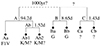 |
Fig. 1. System hierarchy and nomenclature of KIC 4150611, with approximate orbital periods shown in days. Hełminiak et al. (2017) present astrometric evidence for an association between the A and B components, but otherwise the A, B, and C components can be considered dynamically independent. The figure is based on Fig. 15 from Hełminiak et al. (2017). |
This system structure was established in Hełminiak et al. (2017), who conducted velocity modelling of Aa, Ba, and Bb as well as eclipse modelling of the Ab, B, and C binaries. The authors further performed imaging of the system using adaptive optics, establishing it as a visual triple, astrometric measurements searching for long-period dynamical associations, and isochrone fitting based on the properties of Ba and Bb. Detailed eclipse modelling of the A triple can be found in Kemp et al. (2024), along with spectroscopic analysis and atmospheric modelling of the disentangled spectra of Aa, Ba, and Bb.
In this work we build on the previous eclipse and atmospheric analysis of Aa by performing asteroseismic modelling of its g-mode period-spacing pattern, first identified in Li et al. (2020a). Gravity-mode period-spacing patterns are sensitive to interior stellar properties such as near-core rotation rates and buoyancy travel times (Van Reeth et al. 2016; Mombarg et al. 2019) and, when combined with grids of stellar models with computed pulsations, can be used to estimate stellar properties such as masses, ages, and mixing profiles (see, for example, Aerts et al. 2018; Johnston et al. 2019; Pedersen et al. 2021; Mombarg et al. 2021; Michielsen et al. 2023). By considering several different period-spacing patterns and by employing both a pattern-matching approach and a parameter-based grid-search approach that leverages different grids of stellar models, we aim to provide insight into the systematic uncertainty associated with different methods and choices. Attention is also paid to how the different non-asteroseismic measurements that have been made for this system interplay with both each other and the asteroseismology.
We provide a summary of the physical constraints relevant to the asteroseismic modelling of KIC 4150611’s g-mode period-spacing pattern in Sect. 2. We describe our methodology in Sect. 3 and present our results in Sect. 4. We conclude in Sect. 5.
2. Physical constraints from the literature
In this section we provide a brief summary of selected constraints on orbital and stellar properties from the literature relevant to the asteroseismic modelling of Aa. Much of the previous literature relating to KIC 4150611 is dedicated to constraining the orbital properties of the system. These constraints are essential to the identification and extraction of stellar oscillation frequencies as they allow the confident identification of orbital harmonics (see Sect. 3.1).
Using a variety of techniques, several works have provided estimates of the orbital periods of KIC 4150611’s different components (Prša et al. 2011; Shibahashi & Kurtz 2012; Balona 2014; Rowe et al. 2015; Hełminiak et al. 2017; Kemp et al. 2024). For the Ab, B, and C binaries, we made use of the orbital periods from Hełminiak et al. (2017) to aid the identification of orbital harmonics. The complex, time-variant geometry of the 94.2 d eclipses precludes harmonic analysis; these eclipses were removed from the light curve in the time domain prior to the Fourier-space frequency analysis.
From Gaia Data Release 3 (DR3; Gaia Collaboration 2023), we have an estimate for the distance to the system of  pc2, which (using a bolometric3 magnitude of 8.03 for the system) in turn provides an estimate for the system’s luminosity of 7.5 ± 0.3 L⊙ (log(L) = 0.875 ± 0.0175 dex). To make the step from a system luminosity to a stellar luminosity for Aa, we must consider the light fraction of Aa in the system.
The primary makes up most of the light in the system, although estimates of the exact light fraction vary. Kemp et al. (2024) estimate a light fraction of between 0.92 and 0.94 based on spectroscopic analysis of TRES spectra (Szentgyorgyi & Furész 2007) but arrive at a lower value of roughly 0.84 ± 0.03 when considering only the eclipses, a value similar to the 0.85 light fraction obtained by Hełminiak et al. (2017) in their eclipse modelling of the Ab, B, and C binaries. Kemp et al. (2024) consider the effect of this uncertainty on their estimates of system’s properties from their eclipse analysis, noting that the spectroscopic analysis appears far more sensitive to the light fraction than the eclipse modelling and therefore prefer a light fraction of around 0.92. A light fraction of 0.85 implies a log(L) for Aa of 0.804 ± 0.017 dex, while a light fraction of 0.92 implies a log(L) for Aa of 0.838 ± 0.017 dex. We note that the quoted uncertainties only propagate the uncertainty in parallax, and so are lower limits.
From the eclipse modelling in Kemp et al. (2024), the stellar radius for Aa was conservatively estimated as 1.64 ± 0.06 R⊙ when considering the possibility of either a low or high light fraction being true. Both of the Kemp et al. (2024) Markov chain Monte Carlo (MCMC) simulations with constrained light fractions arrive at 1σ uncertainties of approximately 0.01 R⊙.
Hełminiak et al. (2017) provide estimates of several of the properties of Aa properties using isochrone fits to Ba and Bb. These properties include the mass (1.64 ± 0.06 M⊙), radius (1.376 ± 0.013 R⊙), log(g) (4.38 ± 0.01) dex, and effective temperature (8440 ± 280 K). However, isochrone fits suffer from high levels of modelling uncertainty, being tied to the underlying grid of stellar models. Kemp et al. (2024) found poor agreement between their eclipse modelling and the stellar properties estimated from the isochrone fits of Hełminiak et al. (2017), including the radius and mass ratio estimates for the Aa, Ab1, and Ab2 components of the A triple. The effective temperature (Teff) of Aa from the isochrone fits is also too high compared to both the atmospheric modelling conducted in Kemp et al. (2024) and previous spectroscopic analysis from Niemczura et al. (2015). We only used the properties from the isochrone fits for comparative purposes.
The atmospheric modelling on the disentangled spectra of Aa presented in Kemp et al. (2024) estimate Teff = 7280 ± 70 K and log(g) = 4.14 ± 0.18 dex. From the eclipse modelling, there is a deviation from edge-on of at most 0.4°, so the estimate of v sin i = 127 ± 4 km s−1 can be considered simply as the surface rotation. Combined with the conservative estimate of the stellar radius of 1.64 ± 0.06 R⊙ from the eclipse modelling (Kemp et al. 2024), this corresponds to an estimate on the rotation frequency of the surface, Ωsurf, of 1.54 ± 0.1 d−1, where the quoted error encompasses the highest level of disagreement permissible within the 1σ of the radius and surface rotation constraints.
3. Methodology
3.1. Frequency extraction
The process of detrending and obtaining frequencies from KIC 4150611’s complicated photometric time series was discussed in Kemp et al. (2024), but we summarise it again here, as it gives important context to three of the four period-spacing patterns we considered (see Sect. 3.3).
For the purpose of obtaining a g-mode period-spacing pattern for a γ Dor star, Kepler’s long-cadence time-series data are ideal. KIC 4150611 is sparsely observed by TESS and has a considerably poorer signal-to-noise, while short-cadence Kepler data are of little benefit for the low-frequency g-modes of γ Dor stars and add to the computational cost considerably.
Starting from the Kepler long-cadence target pixel files, we employed a custom reduction and instrumental detrending following Van Reeth et al. (2022, 2023). The procedure is designed to improve the available signal while minimising contaminants from other stellar sources and avoid introducing signal from the instrumental detrending. This is achieved by applying a simple linear detrending model to each sector after a rough sinusoid model for the dominant physical effects (typically either eclipses or oscillations) has been subtracted. This is followed by outlier removal through a 5σ clipping and manual inspection. Throughout the detrending process, the 94.2 d eclipses of the A triple were removed from the light-curve. In principle, they could be reintroduced and detrended once the detrending curve was obtained; however, pre-whitening in the frequency domain with these complicated eclipses included in the light curve is impractical and counterproductive.
To obtain lists of frequencies, amplitudes, and phases we iteratively pre-whitened the detrended light curve (with the 94.2 d eclipses removed) using two different methods: manually using period044 and in an automated way using STAR SHADOW5 (IJspeert et al. 2024). Further details of this procedure can be found in Sect. 2.1.1 of Kemp et al. (2024), and the detrended light-curve – and model fit using the STAR SHADOW frequency model – can be seen in Fig. 2. However, it is relevant to highlight certain key differences between the two processes.
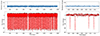 |
Fig. 2. 4-year time series for KIC 4150611. Bottom: Normalised, detrended light curve (black; excluding the 94.2 d eclipses) and the sinusoid model (red) formed from all frequencies extracted using STAR SHADOW. Top: Residuals (blue). Figure 1 of Kemp et al. (2024) shows the equivalent figure for the extracted sinusoid model extracted using period04. |
The first is that while both methods identify orbital harmonics of the 8.65 d, 1.52 d, and 1.43 d eclipses, only STAR SHADOW couples the orbital frequencies for all identified harmonics, leading to a more precise extraction of orbital harmonics. This has relevance due to a near-perfect coincidence between an 8.65 d orbital harmonic and one of the g-modes of KIC 41501611. Figure 3 shows the phase-folded orbital periods using the STAR SHADOW frequencies, and can be compared directly to Fig. 3 from Kemp et al. (2024) and Fig. 2 from Hełminiak et al. (2017), highlighting the consistency of the eclipse extraction.
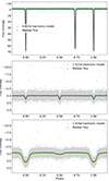 |
Fig. 3. Phase-folded light curves for each of the eclipsing components and its sinusoid model. The light curve (grey data) for each is the residual between the normalised, detrended light curve and every frequency except those forming the sinusoid model of the relevant eclipse from STAR SHADOW. The median flux is shown in green, and the coloured points (colour varies by panel) are from the relevant harmonic model. Figure 3 of Kemp et al. (2024) shows the equivalent figure for the period04 extraction, with no significant eclipse geometry differences. |
The second difference worth highlighting is that, as an automated method, STAR SHADOW employs a strict amplitude-hinting procedure (see, for example, Van Beeck et al. 2021). This means that it proceeds with iterative frequency extraction in descending amplitude order, stopping as soon as the Bayes information criterion reduces by less than two when extracting the next frequency. In contrast, when pre-whitening using period04 the selection of the pre-whitened frequencies is at the discretion of the user, as is the point at which to stop the process. For discussion on different pre-whitening procedures and the influences they can have on the resulting frequency lists, the reader may refer to Degroote et al. (2009) and Van Beeck et al. (2021).
The presence of low-frequency noise in the Fourier transform (commonly referred to as ‘red noise’) can cause frequency extraction to halt before reaching low amplitude – but high S/N – frequencies in the high-frequency domain. This results in the extraction of a lower number of frequencies overall, with high-frequency orbital harmonics clearly appearing in the residuals (see Figs. 4 and 5). The lack of these frequencies does not appear to significantly affect the quality of the orbital harmonic models, however, nor the quality of the pre-whitening in the g-mode regime.
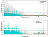 |
Fig. 4. Lomb-Scargle periodogram of the normalised, detrended light curve (grey) with non-orbital harmonic frequencies extracted by STAR SHADOW (light blue) and the periodogram of the residual light curve (orange). The lower panel is the periodogram of the light curve when the orbital harmonics (see Fig. 3) are removed. |
Manual extraction using period04 results in 178 orbital harmonics for the 8.65 d orbital period, 18 orbital harmonics for the 1.52 d orbital period, 19 orbital harmonics for the 1.43 d orbital period, and 1238 other frequencies. STAR SHADOW’s frequency extraction procedure results in 160 orbital harmonics for the 8.65 d orbital period, 15 orbital harmonics for the 1.52 d orbital period, 12 orbital harmonics for the 1.43 d orbital period, and 884 other frequencies. These frequency lists form the basis of our subsequent asteroseismic analysis.
3.2. Period-spacing pattern identification
The objective of this work is to provide asteroseismic analysis of the g-mode period-spacing pattern of KIC 4150611. This pattern is determined in Li et al. (2020a) to be the prograde dipole pattern. The low-frequency gravito-inertial modes detected in our target are often called prograde dipole modes, deriving from the limited notation (l, m) = (1, +1) in terms of spherical harmonics for reasons of simplicity; in reality this spherical harmonic component delivers only the dominant contribution to the actual Hough eigenfunction (Hough 1898) of such modes. For this reason, Lee & Saio (1997) introduced the more general notation (k, m) = (0, 1) for such modes, where k ≡ l − |m|.
We considered four different period-spacing patterns to evaluate how different extraction processes and pattern identification decisions can affect our results. The first was the Li et al. (2020a) pattern, which we did not modify in any way. This pattern was also constructed from long-cadence Kepler data, but with a different light curve extraction and detrending process. Notably, the algorithm of Li et al. (2020a) applied a relatively low S/N threshold of 3 when considering the significance of each frequency. We refer to this pattern as the PAT_LI2020 pattern.
To construct period-spacing patterns from our own various light curves and their pre-whitened frequency lists, we employed an iterative procedure, manually identifying candidate pattern members in the region of the Lomb-Scargle periodogram (Lomb 1976; Scargle 1982) relevant to γ Dor stars and (re-)fitting a theoretical asymptotic period-spacing pattern produced by AMiGO6 (Van Reeth et al. 2016, 2018), which relies on the numerical approximations worked out by Townsend (2020).
AMiGO computes theoretical period-spacing patterns assuming a rigidly rotating, chemically homogeneous star under the traditional approximation of rotation (TAR; Eckart 1960; Berthomieu et al. 1978; Lee & Saio 1989, 1997; Mathis 2009; Bouabid et al. 2013; Van Reeth et al. 2016). Under the TAR, the horizontal component of the rotation vector is neglected, rendering the oscillation equations separable in spherical coordinates. The effect of rotation on the radial and azimuthal displacements are neglected while in the latitudinal direction they can be computed by solving the Laplace tidal equation, for which solutions can be expressed in terms of Hough functions (Hough 1898). This achieves the accuracy required for the modelling of observed low-frequency modes in rotating stars, in contrast to perturbative asymptotic predictions (see, for example, Shibahashi 1979). Indeed, given the significant frequency shifts induced by the Coriolis acceleration (see, for example, Figs. 3 and 4 in Aerts & Tkachenko 2024), one should not approximate gravito-inertial modes from computations in the perturbative regime.
The TAR is valid for modes where the displacement vector is dominant in the horizontal plane, which is an excellent approximation for γ Dor stars (Aerts 2021), including KIC 4150611. For the majority of these pulsators, the modes in the co-rotating frame have a frequency less than twice the rotation frequency, and the stellar rotation frequency is much less than both the Brunt-Väisälä and Lamb frequencies, which govern the stability of buoyant and acoustic restoring forces, respectively, to allow for mode propagation (Aerts & Tkachenko 2024). This allows for asymptotic period-spacing patterns to be computed as a function of the rotation frequency in the near-core region, Ωc, and the buoyancy travel time, Π0, originally defined by Tassoul (1980):
 (1)
(1)
where N is the Brunt-Väisälä frequency and r1 and r2 are the boundaries of the mode cavity. The frequencies of the g-modes belonging to a period-spacing pattern of known degree l and azimuthal order m can then be computed according to
 (2)
(2)
where λlm, s is the mode-specific eigenvalue of the Laplace tidal equation and α is a phase term determined by the details of the mode-cavity boundaries, usually treated as a free parameter (around 0.5 in γ Dor stars) in practice (Bouabid et al. 2013; Van Reeth et al. 2015a, 2016). The value of λlm, s is determined for each oscillation frequency by its spin parameter s = 2Ωc/ωlmn, where ωlmn is the mode’s angular frequency in the co-rotating reference frame.
AMiGO determines λlm, s using GYRE’s ‘lambda(nu)’ function, first sampling a grid over a frequency domain appropriate to the star and then interpolating to determine precise values of λlm, s of each mode. In this way, AMiGO is able to quickly produce asymptotic period-spacing patterns for high-order gravito-inertial modes as a function of Ωc and Π0.
By computing a grid of such patterns varying Ωc and Π0 and comparing with an observed period-spacing pattern, best-fitting values and uncertainty estimates for Ωc and Π0 can be obtained without computing detailed stellar and asteroseismic models. In addition to being faster, this has the advantage of avoiding unpredictable systematic errors due to uncertainty in the details of the input physics of stellar models. However, by the same token, the links between these predictions and the physics of stellar interiors is absent, limiting the inferences that can be drawn directly. Furthermore, as a natural consequence of the underlying physical assumptions in the approach, structural information present in the pattern due to chemical gradients and other neglected physics cannot be reproduced. In stars where the structural variations throughout the interior are large and induce deviations from a smooth period spacing pattern, the accuracy of the stellar parameters inferred via methods such as AMiGO will be limited. This is not a concern in the case of KIC 4150611, where we observe a very smooth period-spacing pattern.
In addition to its utility in providing estimates of Ωc and Π0 (see Sect. 4.2), pattern predictions from theoretical frameworks such as AMiGO provide a useful aid in the identification of oscillation frequencies that may form part of a period-spacing pattern, as highlighted by Van Reeth et al. (2015a). Starting from obvious pattern members, we used AMiGO’s pattern predictions as a guide to assist in identifying additional candidate pattern oscillations, which we then fed back into AMiGO in an iterative process.
In this manner, we arrived at three period-spacing patterns (in addition to the previously identified pattern in Li et al. (2020a): two from the frequency list extracted using period04 and one from the frequency list extracted using STAR SHADOW. All patterns are included for ease of comparison in Fig. 6. The first pattern we obtained from the period04 pre-whitening process was extracted in a deliberately pessimistic manner, only taking frequencies that have S/N strictly above 5.6 (Baran et al. 2015) and are not ambiguous. The result is a pattern with several gaps and only short segments of consecutive modes, particularly at longer periods (equivalent to higher radial order n). This pattern represents a pessimistic pattern selection, and we refer to it as PAT_P04_PES.
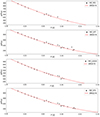 |
Fig. 6. Period-spacing patterns considered in this work, along with their AMiGO fits. |
The second pattern from the period04 frequency list is obtained by selecting frequencies in a deliberately optimistic manner. In this selection, we allowed moderate deviations below a S/N of 5.6 in an attempt to build the largest pattern possible. This included judging whether a given mode is real and of stellar origin not only based on the mode’s own properties – such as its S/N – but also making use of prior knowledge of the existing pattern. The result is a more complete period-spacing pattern that extends to higher radial order modes than both the PAT_LI2020 and PAT_P04_PES patterns. We refer to this pattern as PAT_P04_OPT.
The final pattern makes use of the STAR SHADOW frequency list and is also obtained in an optimistic manner, allowing moderate deviations in S/N for modes that fit the rest of the pattern. The resulting pattern is similar in length and completeness to PAT_P04_OPT, although the different extraction procedure results in differences to the extraction of low amplitude, high-order modes relevant to the pattern. We refer to this pattern as PAT_STS.
Further details about the extraction characteristics in the period region surrounding PAT_LI2020, PAT_P04_OPT, PAT_P04_PES and PAT_STS are shown visually in Figs. A.1–A.4. The top panel of each figure shows the extracted frequencies, Lomb-Scargle periodogram for the relevant light curve with eclipse harmonics excluded, and the residual periodogram. The predicted frequencies from the AMiGO fit to the pattern are also shown, as well as the S/N and estimated errors in amplitude and period for each extracted mode. In Fig. A.1, the extracted frequencies, Lomb-Scargle periodogram, and residuals shown are from the period04 frequency list for comparison with the PAT_LI2020 period-spacing pattern, which is plotted along the x-axis. In all figures, the lower panels show the period-spacing pattern and relevant AMiGO fit to each pattern.
We note that while they are not shown in Figs. A.2–A.4, orbital harmonics, alias frequency predictions, and linear combinations of high-amplitude mode pairs were taken into account during pattern identification. Although there are several alias frequencies that fall within the domain of the period-spacing pattern, particularly those relating to the 94.2 d orbit, none fall close enough to selected modes to be of concern.
There is a near-perfect coincidence between one of the 8.65 d orbital harmonics and the extracted high-amplitude mode at 0.37 d (this is excluded for this reason in the PAT_P04_PES pattern, but included in the PAT_LI2020, PAT_P04_OPT, and PAT_STS patterns). This is the cause of the non-physical oscillatory behaviour that appears in the 8.65 d phase-fold when using the period04 frequency list to construct harmonic models of the eclipses discussed in Kemp et al. (2024). This is avoided in the STAR SHADOW extraction due to the enforcement of frequency-coupling between orbital harmonics. However, when comparing these patterns in Fig. 6 (see also Figs. A.3 and A.4), it is clear that this makes little difference to the period-spacing pattern; the two patterns are essentially identical in the high-amplitude region below 0.4 d.
All four patterns exhibit similar behaviour in the high-amplitude, short-period region. Differences only start to become noticeable when considering the low-amplitude, long-period modes. The PAT_LI2020 period-spacing pattern’s second consecutive mode sequence (between approximately 0.4 and 0.43 d) is very regular, but relies on extremely low-amplitude modes. Interestingly, it is the location of the second mode in this sequence – one of the relatively high S/N modes – that is the most noteworthy deviation when comparing with the PAT_P04_OPT and PAT_STS patterns. This mode is shifted slightly towards a lower period in both the STAR SHADOW and period04 frequency lists. The structure of the third consecutive sequence, between 0.43 d and 0.46 d, is essentially identical between all frequency lists.
PAT_P04_PES, PAT_P04_OPT, and PAT_STS all include modes beyond the third and final sequence of PAT_LI2020, although in the case of PAT_P04_PES this includes very few consecutive modes. Beyond the high amplitude peak at approximately 0.46 d, there is a low amplitude valley followed by a high-amplitude peak. Several of these modes do not satisfy S/N > 5.6, and the predicted mode density in this region is approaching levels where chance coincidences of individual observed periods with the predicted would be a concern. Nonetheless, a series of modes with spacings consistent with the AMiGO predictions can be found here, noting that extracted frequencies in this region are different in places between the PAT_STS pattern and the PAT_P04_OPT pattern to the point where it appreciably affects the structure.
At this point, it is worth noting how the AMiGO fit predictions are used. Simply comparing the period predictions to the locations of extracted modes is often unhelpful, as individual oscillation periods can be affected by the chemical gradients inside the star. These period shifts manifest as structural glitches in the period-spacing pattern before quickly returning to the asymptotic behaviour, and are not able to be modelled by AMiGO. The structural glitch seen in the third consecutive sequence in PAT_LI2020, PAT_P04_OPT, and PAT_STS is an example of such a mode shift (around radial order 34 in Fig. 7).
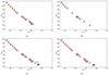 |
Fig. 7. Best-fitting C-3PO models (red) consistent with the radial and spectroscopic constraints (see Table B.1): PAT_LI2020 (a), PAT_P04_PES (b), PAT_P04_OPT (c), and PAT_STS (d). Observed patterns are shown in black. |
It is clear that the inclusion – or not – of these high-order modes in the pattern has a much larger effect on the AMiGO fits than the differences in the actual mode frequencies between the different patterns. PAT_LI2020 and PAT_P04_PES have relatively similar AMiGO fits, which rely far more upon the highest amplitude, short-period modes. Conversely, despite the structural differences between PAT_P04_OPT and PAT_STS at high radial orders, the fit between the two is near identical. As AMiGO only includes the physics needed for modelling the overall pattern shape, this is anticipated.
3.3. Asteroseismic grid modelling
The most expensive aspect of asteroseismic modelling using g-modes is undoubtedly the computation of grids of stellar models and their pulsations. In order for the resolution of the grid not to adversely affect the results, dense stellar grids are required. These grids must, at minimum, span the zero-age main sequence mass and an age proxy such as the central hydrogen mass fraction, Xc. As the tilt of a period-spacing pattern is highly sensitive to the near-core rotation frequency Ωc, dense sampling of this parameter is required when computing the pulsations if the pattern is to be compared with directly. The required sampling density of Ωc can be reduced by optimising the rotation scaling independently as part of the merit function, essentially finding the most probable Ωc for each structural model (see Michielsen et al. 2023). However, probing other additional stellar physics such as convective boundary mixing parameters, for example the degree of step (Shaviv & Salpeter 1973; Zahn 1991) or exponential (Freytag et al. 1996; Herwig 2000) overshooting, involves adding, for each factor, a dimension to a grid of stellar models, which multiplies the computational cost.
In this work, we made use of C-3PO7, a neural-network-driven asteroseismic modelling code for γ Dor stars (Mombarg et al. 2021). It rapidly makes predictions for the pulsation frequencies, period-spacings, and radial-orders of a star based on its mass M, Xc, metallicity Z, Ωc, and degree of exponential core overshooting fov. This is accomplished by taking the average frequency prediction from five different neural networks dedicated to this task. A separate neural network computes Teff and log(g), common physical constraints from spectroscopy, while another computes the luminosity L for each model, which can then be compared with astrometric luminosities such as those from Gaia (Gaia Collaboration 2016). The underlying stellar structure and pulsation models used to train C-3PO were computed using MESA (Paxton et al. 2013) and GYRE (Townsend & Teitler 2013), respectively. Despite not including rotation explicitly, the training set used for C-3PO used stellar models computed with a constant envelope mixing (Dmix = 1 cm2 s−1) to account for transport processes in the envelope. This low level of Dmix reflects the low levels of envelope mixing found in γ Dor stars (Van Reeth et al. 2016; Mombarg et al. 2019). The training set includes a diffusive-exponential core overshoot prescription, varying the diffusive exponential overshoot factor, fov, between 0.01 and 0.03. The training set spans the γ Dor range in mass (1.3–2.0 M⊙) and spans a small range of metallicities around solar (Z = 0.011 − 0.015). Further details of the underlying physics of the MESA models and GYRE pulsation models on which the network is trained can be found in Mombarg et al. (2021).
In addition to the neural network predictor modules, C-3PO includes a modelling framework that handles both radial-order matching using the neural network’s pulsation predictions and assigning merit values for each model. The period-spacing patterns are built by matching the first period in the longest sequence of consecutive modes, and building out the pattern to the other sequences from there. The merit function includes both the periods and the period spacings; this can be viewed as a compromise between constraining power and sensitivity to un-modelled physics. Michielsen et al. (2021) find that, for their case-study star of KIC 7760680, a slowly pulsating B star with an exceptionally long period-spacing pattern with a high level of structure, a merit function accounting only for the periods is inferior to one accounting only for mode period spacings, citing high variance in theoretical mode predictions for the pulsation periods. By combining both period-spacings and periods, C-3PO’s methodology attempts to ensure that period-spacings are accurately fit, while rewarding models that also have agreement in the mode periods.
Michielsen et al. (2021) also compare two merit functions: the commonly used χ2 and the Mahalanobis distance (MD; Johnson & Wichern 2019) with an additional term for the model variance (Aerts et al. 2018). This additional term adjusts the weight given to each observation according to both the degree of covariance between each observable according to the model grid – in this way attempting to measure the modelling uncertainty – on top of the covariance between the observables themselves. This results in a broadening of the parameter space, widening uncertainty regions. Michielsen et al. (2021) find that the MD-based merit function outperforms the χ2 merit function insofar as it arrives at more realistic uncertainties. However, an important caveat is that KIC 7760680 had an unusually long and complete period-spacing pattern with prominent structures that could be mostly explained by physics included within the underlying pulsation models.
Preliminary analysis on KIC 4150611 making use of the forward modelling software package Foam (Michielsen 2024) revealed that use of the MD-based merit function led to poor fits to the period-spacing pattern regardless of whether the period-spacing or the periods were fit. Patterns that vaguely approximated the structural glitches in the period-spacing pattern strongly preferred despite those models utterly failing to reproduce the rest of the pattern. The χ2 statistic, on the other hand, placed no special weight on those structures, instead favouring patterns that matched the observed pattern as a whole.
C-3PO supports both the χ2 and the MD-based merit function merit functions; we made use of the χ2 for KIC 4150611. C-3PO’s modelling framework also supports using external constraints such as Teff, log(g), and L in the sampling phase, which can allow for a more efficient sampling of the relevant space. We did not make use of this feature, instead opting to compute many models uniformly distributed across the entire γ Dor range. This is to facilitate discussion of the relative constraining power of asteroseismic, spectroscopic, and eclipse-modelling observables and their combinations for different stellar parameters. To assess the impact of sampling effects on our results, we computed our results using two different samples for each pattern: a medium resolution sample, with 8 × 10⁵ models across the γ Dor range, and a high resolution sample, with 3 × 10⁶ models. We present the results from the high resolution sampling in the main text, while the results from the alternative ‘Tight R’ radius constraint in the appendices. All figures relating to the medium resolution sampling are included in the online supplementary material. A summary of the different configurations of external constraints considered is presented in Table 1.
External constraints and labelling conventions.
We estimated the uncertainty for our C-3PO modelling by estimating a 1σχ2 cutoff using Eq. (9) from Mombarg et al. (2021), and then taking the maximum and minimum parameter values from that distribution to form the 1σ estimate. These uncertainty estimates should be treated with caution, particularly for cases where the parameters do not have normal (or even quasi-normal) χ2 envelopes. Furthermore, the 1σ subsamples these margins are based on contain relatively few (20–40) models in the most constraining case, adding an element of stochasticity to their estimation.
3.4. MCMC parameter-based grid search
To better understand the correlations between and the uncertainty structure of our parameter estimates, we also employed a classical MCMC grid search. This was done using several different grids of stellar models (grids A–E):
-
Grid A: a grid composed of the lowest metallicity non-rotating models from Mombarg et al. (2021) (the same underlying models used to train C-3PO).
-
Grid B: a grid composed of solar-metallicity, rotating stellar models from Mombarg et al. (2024a) (employing hydrodynamic envelope mixing and angular momentum transport based on the rotation, as well as microscopic diffusion).
-
Grid C: a grid of rotating solar metallicity models from Mombarg et al. (2024b) (employing rotational mixing but with fixed viscosity and no microscopic diffusion).
-
Grid D: a grid of Z = 0.0045 models also from Mombarg et al. (2024b).
-
Grid E: a grid of Z = 0.008 models with physics equivalent to Mombarg et al. (2024b) (Aerts et al. 2024).
We note that although the grid of low-metallicity models from Mombarg et al. (2021) is from the same set used to train C-3PO, it is considerably denser, as C-3PO was trained only on the subset of stellar models where GYRE pulsation models were computed.
The grid search employed an MCMC sampling method similar to Fritzewski et al. (2024) based on the external constraints Teff, R, L, log g, and the asteroseismic measurement of the buoyancy travel time parameter Π0. For the rotating stellar models, the asteroseismic near-core rotation Ωc was also used. We allowed the MCMC walkers to explore the grid in three unconstrained parameters M, fov, and Xc while keeping the envelope mixing fixed to Dmix = 1 cm2 s−1. We assumed a flat prior for all parameters.
4. Results
In this section we present the results of our asteroseismic modelling of the g-mode period-spacing pattern of KIC 4150611 Aa.
4.1. Pattern fits
The best-fitting models to the relevant period-spacing patterns that satisfy the radius and spectroscopic constraints are included in Fig. 7. These best-fitting models fit the overall shape and location of the periods and period-spacing patterns satisfactorily, and subtle structural features in the observed patterns are able to be modelled in many cases. The fact that the fits make no effort to model the stronger dips and features in the observed patterns is reassuring, as it implies a level of resilience of the methodology to un-modelled physics or badly extracted frequencies (the two are functionally identical and often indistinguishable from a modelling perspective). The quality of the fits, including the apathy towards the larger structural features, is very similar when considering the best overall asteroseismic fit without considering external constraints, as opposed to the best constrained fit shown in Fig. 7.
An interesting example of the models’ ability to reproduce the small-scale structure is the fit to the PAT_LI2020 pattern from radial orders 25–29 in Fig. 7a. The structure here is only slight, but is able to be reproduced very well by the model. What makes this segment particularly interesting is that the same structure reappears in the fits to the other period-spacing patterns, which include a glitch around the spacings of the 25th and 26th radial order modes. This implies that this structure is an inevitable consequence of matching other parts of the pattern well, most likely the robust first segment (radial orders 16–22). This in turn leads to the conclusion that, at least for this segment, the PAT_LI2020 pattern is most likely the correct accurate extraction despite our inability to reproduce its structure in any of the other three patterns.
In contrast, the structure of the third segment (the spacings of radial orders 32–36) is consistent between all three patterns where it was able to be extracted (PAT_LI2020, PAT_P04_OPT, and PAT_STS). In all three cases, it is dominated by a large glitch that is not reproduced by our current models.
Beyond this sequence, only the PAT_P04_OPT and PAT_STS patterns are worth discussing, as PAT_LI2020 does not extract beyond the third sequence and PAT_P04_PES extracts only the spacing for the 39th radial order mode. Both PAT_P04_OPT and PAT_STS include four consecutive modes at high radial order, although the modes extracted differ between the two patterns: PAT_P04_OPT includes spacings for the radial orders 43–45, while PAT_STS includes the spacings of radial orders 44–46. The common radial orders between both patterns, n = 44 and n = 45, are in agreement and reproduced by their models. However, while the n = 46 mode is reproduced by the model fitting the PAT_STS pattern, the n = 43 mode in the PAT_P04_OPT pattern is not. Considering its low amplitude, we consider its detection spurious.
4.2. Parameter estimates
Figures B.1–B.4 show the results of the parameter estimation component of our modelling work when considering our default case of conservative external constraints. The upper triangular panels present heat maps (with darker colours representing better fits) tracking the maximum of the 1/χ2 merit function considering all samples, irrespective of external constraints. The panels on the main diagonal present distributions and envelopes of the 1/χ2 merit function for each parameter, as well as the best-fitting models when considering different external constraints (see Table 1). Finally, the lower triangular panels are ‘scatter pies’8 showing how the different external constraints (see Table 1) manifest in each 2D projection of the landscape, with the best-fitting models for each external constraint also shown. Further guidance on reading these figures can be found in the figure caption of Fig. B.1, and the parameters of the best-fitting models for each pattern and each external constraint are tabulated in Table B.1.
Before we delve deeper into each parameter, it is informative to make a few general comments about the results obtained for each pattern. The first thing to note is that the best-fitting model for the PAT_P04_OPT and PAT_STS patterns, while different between each pattern, is the same when considering the asteroseismology in an unconstrained manner and when considering both the radius and spectroscopic constraints. This is not the case for the PAT_LI2020 and PAT_P04_PES patterns; in the PAT_LI2020 pattern, the best-fitting asteroseismic solution satisfies the spectroscopic constraint but not the radius constraint, while for the PAT_P04_PES pattern, the best-fitting asteroseismic solution does not satisfy any of the external constraints. Although this could be coincidence, this can be easily understood by considering that the PAT_P04_OPT and PAT_STS patterns contain the most identified spacings, and are therefore more constraining than the shorter PAT_LI2020 and PAT_P04_PES patterns.
The other general comment to be made is that in every case, the best-fitting model from the subset that satisfies the relevant radius constraint (either the tight constraint or the more conservative default constraint) also satisfies the spectroscopic constraints on Teff and log(g). This is in spite of the fact that, as can be seen from the lower triangular panels of Figs. B.1–B.4, for many parameters the radius and spectroscopic external constraints have near-orthogonal intersections.
We now discuss each parameter, beginning with those for which calculations can be made can be made without relying on grids of stellar models (Ωc and Π0), followed by the model-dependent parameters that are directly obtained from the modelling framework (M, Xc, Z, fov, Teff, log(g), and log(L)) and finally the stellar age, which we estimated from the underlying training sets, and the stellar radius, which we calculated for each model using the stellar mass and its surface gravity.
4.2.1. Near-core rotation frequency
As previously explained, the near-core rotation frequency and buoyancy travel time can be directly obtained from the period-spacing patterns without comparison with detailed stellar pulsation models by using a purely theoretical framework. Under the assumptions described in Sect. 3.2, theoretical patterns depending on Ωc and Π0 were computed using AMiGO and fit to the observed period-spacing pattern, providing both best-fitting values and an uncertainty estimate for these two parameters. The best-fitting asymptotic patterns to each observed period-spacing pattern can be found in Fig. 6. For the PAT_LI2020 pattern, we obtain an estimate for the near-core rotation rate of Ωc = 1.562 ± 0.016 d−1, while the other three patterns give estimates of approximately 1.577 ± 0.010 d−1. These results are consistent with the 1.58 ± 0.01 Ωc estimate from Li et al. (2020a).
Previously, in Sect. 2, we estimated the surface rotation frequency for Aa using the radius and radial velocity estimates from Kemp et al. (2024) to be Ωsurf = 1.54 ± 0.10 d−1. Using our Ωc estimate of 1.58 ± 0.01, we can conservatively estimate the surface-to-core rotation fraction as: Ωsurf / Ωc = 0.975 ± 0.064. This is consistent with the picture of quasi-rigid core-to-surface rotation presented in Fig. 6 of Aerts (2021) for main sequence F-type stars. Aa’s Ωc of approximately 1.58 d−1 (18 μHz) and log(g) of 4.14 ± 0.18 (Kemp et al. 2024) place it in the middle of the well-populated clump of other rapidly rotating F-type stars.
As a final comment, we note that it is possible to relax the assumption of rigid rotation, and instead consider a theoretical asymptotic pattern accounting for slightly radially differential rotation within the star (Ogilvie & Lin 2004; Mathis et al. 2008; Mathis 2009; Van Reeth et al. 2018). However, inferring differential rotation in stellar interiors in this way requires either rotational mode-splittings on top of a period-spacing pattern (e.g. as in Triana et al. 2015; Schmid & Aerts 2016) or the characterisation of multiple period-spacing patterns within the star to break the degeneracy with rigid rotation (Van Reeth et al. 2018). In Van Reeth et al. (2018), it was concluded that for all but the most extreme cases of differential rotation, only stars exhibiting period-spacing patterns in both prograde-dipole and Rossby modes have sufficient distinguishing power to unravel differential from rigid rotation. In KIC 4150611, we identified neither rotational mode splitting – even in the high-amplitude p-modes – nor a reliable9 additional period-spacing pattern, precluding further conclusions of the level of differential core-to-envelope rotation other than to say that the rotation is rigid to within the measurement errors when comparing the asteroseismic near-core rotation and the surface rotation derived from spectroscopy.
4.2.2. Buoyancy travel time
Similarly to Ωc, the buoyancy travel time Π0 can be estimated directly from AMiGO’s fit to the pattern using the TAR (see Sect. 3.2). For all patterns except the PAT_LI2020 pattern, AMiGO estimates Π0 to be approximately 4024 ± 74 s; for the PAT_LI2020 pattern, similarly to Ωc, a slightly lower Π0 with a higher uncertainty is obtained (Π0 = 3941 ± 112 s). These estimates are consistent with the Π0 estimate of 4050 ± 80 s from Li et al. (2020b). We return to the question of the stellar age later, but if Aa was very young (as suggested by Hełminiak et al. 2017’s isochrone fitting) we would expect a significantly higher Π0 (Π0 > 4400 s).
4.2.3. Stellar mass
Due to the importance of stellar mass in determining so much of stellar evolution, it is of particular interest to obtain an estimate. Obtaining a precise constraint is difficult in γ Dor stars due to degeneracies with Xc and Z (Mombarg et al. 2019). There is indeed significant variation in this parameter when considering the best-fitting models for each pattern and the different external constraints (see Table B.1).
Considering first the pure asteroseismology, (the ‘All’ case, where all models are considered), we can see that the envelope for the stellar mass is quite flat for all patterns, implying poor constraining power. This is reflected in the uncertainty estimates, which span the entire γ Dor region. Considering only the best-fitting values, the less constraining PAT_LI2020 and PAT_P04_PES patterns arrive at best-fitting models with relatively high mass, 1.96 M⊙ and 1.69 M⊙, respectively. The more constraining PAT_P04_OPT and PAT_STS models arrive at lower mass best-fitting models, at 1.506 M⊙ and 1.512 M⊙, respectively. It is clear from the envelopes that obtaining a confident mass estimate from asteroseismic observables alone for KIC 4150611 is impossible even for the longer period-spacing patterns.
Examining the lower triangular panels of Figs. B.1–B.4, it is clear that in isolation the radius and spectroscopic constraints each provide little information on the mass, with each spanning most of the considered parameter space. When considered together, however, a near-orthogonal intersecting region is produced that, even with our conservative (2σ) constraints on the stellar radius, Teff, and log(g), constrains the stellar mass to between 1.4 and 1.6 M⊙. Enforcing the tight radius constraint (1.64 ± 0.01 R⊙) offers only a slight improvement.
When considering all observables together, the best-fitting models for all period-spacing patterns have masses between 1.47 and 1.51 M⊙, with PAT_LI2020 and PAT_P04_PES favouring a lower mass estimate around 1.47–1.48 M⊙ and PAT_P04_OPT and PAT_STS favouring a slightly higher mass around 1.50–1.51 M⊙. The medium resolution sampling arrives at very similar results: 1.46–1.51 M⊙, and the same bifurcation between the PAT_LI2020/PAT_P04_PES and PAT_P04_OPT/PAT_STS patterns. Typical 1σ error estimates are approximately ±0.05 M⊙ when considering only the subsample of models satisfying the external constraints. Enforcing a tight radius constraint changes little, with the various patterns still arriving at best-fitting stellar models with stellar masses between 1.47 and 1.50 M⊙, while the bifurcation between the PAT_LI2020/PAT_P04_PES and PAT_P04_OPT/PAT_STS solutions disappears. Considering the variation in the best-fitting models, we arrive at a precision of better than 2% in mass.
4.2.4. Core hydrogen fraction
The core hydrogen fraction is a proxy for the stellar age, a property of particular interest for KIC 4150611. Hełminiak et al. (2017) estimate the age of the B binary (two G stars) to be approximately 35 Myr from isochrone fitting. Considering the large number of eclipses in an otherwise uncrowded field and the tentative dynamical association between the A triple and the B binary (Hełminiak et al. 2017), the co-evolution assumption is well motivated for KIC 4150611. Under this assumption, an asteroseismic estimate of Xc parameter can be used to put this previous age to the test. A 35 Myr age for KIC 4150611 would imply that Aa is the youngest γ Dor star observed to date. We will return to the stellar age after concluding our discussion on C-3PO’s directly modelled parameters.
Firstly, it is important to note that the stellar mass and Xc are highly correlated in the asteroseismic fits, reflected in the strong banding present in the 2D envelope seen in the upper triangular panels showing Xc versus M in Figs. B.1–B.4. For this reason, much of the previous discussion surrounding M is relevant to Xc.
Once again first considering the pure asteroseismic estimations, due to the correlated nature of Xc and M the high mass estimates of the PAT_LI2020 and PAT_P04_PES patterns translate to low estimates of Xc, with the converse true for the PAT_P04_OPT and PAT_STS patterns. Furthermore, we note that once again the envelope is mostly flat, and therefore poorly constraining, with the 1σ error estimate once again spanning almost the entire range of possible values of Xc (0–0.7). Considering the external spectroscopic and eclipse modelling constraints without the benefit of asteroseismology, a fairly broad bounding constraint between 0.38 and 0.58 in Xc can be placed10.
Considering the external constraints and the asteroseismology in conjunction, we see that the best-fitting models have Xc varying between 0.42 and 0.49 from the high resolution sampling, with PAT_LI2020 and PAT_P04_PES favouring higher Xc and PAT_P04_OPT and PAT_STS favouring lower Xc, as expected given their preferences towards a higher stellar mass estimate. Estimated 1σ uncertainties for these constrained values are at most ±0.1, and appear to be significantly lower for some patterns (±0.04 in the case of PAT_STS, for example). Enforcing the tight radius constraint results in the best values for Xc between 0.42 and 0.44.
4.2.5. Metallicity
The sampling in Z is low resolution, with only 5 different cases able to be considered over a narrow range (Z = 0.011 − 0.015). There does, however, seem to be a preference towards lower metallicity solutions, especially when the radius and spectroscopic constraints are taken into consideration, although the envelope is very flat.
From atmospheric analysis of the disentangled spectrum of Aa in Kemp et al. (2024), we have a metallicity estimate of [M/H] = − 0.23 ± 0.06, corresponding to Z = 0.0084 ± 0.0011 (using the solar metallicity of Z⊙ = 0.0142857 from Asplund et al. 2009, following Mombarg et al. 2021). This places the star in the middle of the metallicity range of γ Dor stars with metallicity measurements from high-resolution spectroscopy (Gebruers et al. 2021). This metallicity is slightly outside the bounds of the training set for C-3PO, which has a lower limit of 0.011. Armed with the knowledge of the spectroscopic metallicity measurement, we note that the preference towards lower metallicity could imply a small degree of sensitivity to Z in the asteroseismic fits. However, precise estimation of metallicity from g-modes in isolation is unlikely to be possible in practise due to degeneracy between the stellar mass and metallicity.
4.2.6. Exponential overshooting factor
The exponential overshooting factor determines the degree of exponential core overshooting in the core boundary region. Mombarg et al. (2021) vary this from between 0.01 and 0.03 to form their training set.
For all patterns except PAT_P04_OPT, which has a (very flat) ‘U’ distribution spanning the full range of fov, there is a clear preference towards low exponential overshooting. This is consistent with the empirical M–fov relation of Claret & Torres (2017), who found values of fov between 0.005 and 0.02 across the γ Dor range, with lower values associated with the low-mass end regime 1.4–1.5 M⊙. We note that Mombarg et al. (2024a) find no such correlation between the stellar mass and fov, but do find that low values of fov are most probable in γ Dor stars.
Despite the fact that fov can affect the stellar radius and other external properties such as the luminosity, we find that the radius and spectroscopic constraints provide no useful constraint on this parameter. This is true regardless of whether we consider our constraints in isolation or together.
4.2.7. Effective temperature and surface gravity
From atmospheric analysis on the disentangled spectra using GSSP (Tkachenko 2015), we have an estimate for the effective temperature and surface gravity of Teff = 7280 ± 70 K (log(Teff) = 3.8621 ± 0.0042 dex) and log(g) = 4.14 ± 0.18 dex.
A centrally peaked envelope around (approximately) the spectroscopic solution is present with or without external considerations for all patterns, although the PAT_P04_OPT pattern’s envelope is significantly flatter and broader. The best-fitting log(Teff) solutions – excluding the extreme case of log(Teff) = 3.843 dex for the PAT_P04_PES pattern considered without external constraints – vary from between 3.855 and 3.856 dex, placing them slightly below the lower bound of the 1σ uncertainty of the GSSP estimate. Considering that the effective temperature was not part of the merit function, this level of agreement is quite good, although we note that the best-fitting models for all patterns slightly under-predict the spectroscopic solution. Uncertainty estimates for the upper limit of log(Teff) can be as high as +0.008 dex, and are even larger when considering lower temperatures (approximately −0.012 dex). These uncertainties are sufficiently large that they overlap with the spectroscopic estimate for Teff.
Spectroscopy only places loose constraints on log(g) (log(g) = 4.14 ± 0.18 dex, Kemp et al. 2024), with the 2σ uncertainty region essentially spanning the entire γ Dor range. However, the radius constraint from the eclipse modelling narrows the viable region considerably. Combining the spectroscopic and radius constraints allows bounding constraints to be placed on log(g) of 4.15–4.25 dex, consistent with the spectroscopic solution. Within this far smaller region, the envelope of the asteroseismic merit function is peaked, although the best-fitting solution still varies significantly from pattern to pattern. PAT_LI2020 and PAT_P04_PES arrive at higher estimates for log(g), 4.206 dex and 4.223 dex, respectively, while the best-fitting solutions for PAT_P04_OPT and PAT_STS arrive at log(g) of 4.168 dex and 4.176 dex, respectively. For all patterns, a slightly higher log(g) than the face value of the spectroscopic solution is preferred, although all three cases are, as a result of the already constraining intersection between the radius and spectroscopic solutions, well within the spectroscopic 1σ uncertainty region. Typical 1σ uncertainties of the constrained asteroseismic modelling are estimated to be approximately ±0.04 dex.
4.2.8. Luminosity
The luminosity χ2 envelope is, similar to log(g), characterised by a broad and relatively flat envelope when considering the asteroseismology in isolation. The spectroscopic constraints affect this little, although it is interesting to note that, when looking at the histogram of the asteroseismic merit function, the peak roughly coincides with the region consistent with the intersection between the spectroscopic and radius constraints.
Also similar to log(g), imposing both the spectroscopic and radius constraints allows bounding constraints to be placed on log(L) (0.7–0.9 dex). PAT_LI2020 and PAT_P04_PES arrive at lower estimates for log(L) of 0.763 dex and 0.745 dex, respectively, while the best-fitting solutions for PAT_P04_OPT and PAT_STS arrive at estimates for log(L) of 0.819 dex and 0.809 dex, respectively. Estimated 1σ uncertainties are approximately +0.006 and −0.003 for the externally constrained asteroseismic solutions.
From Gaia DR3, we have log(L) estimates for Aa of log(L) = 0.804 ± 0.017 dex assuming a light fraction of 0.82, and log(L) = 0.838 ± 0.017 dex assuming a light fraction of 0.92 (see Sect. 2). Considering our best-fitting solutions, the lower values of the PAT_LI2020 and PAT_P04_PES solutions for log(L) (0.763 dex and 0.745 dex, respectively) are closer to, but still underestimate, even the lower light fraction (0.85) luminosity estimate preferred by the eclipse modelling and Hełminiak et al. (2017). The higher values of log(L) implied by the best-fitting solutions of the PAT_P04_OPT and PAT_STS patterns (0.819 dex and 0.809 dex), however, are consistent with the Gaia luminosity regardless of which light fraction is assumed.
4.2.9. Stellar age
The stellar age can be estimated from the mass and core hydrogen fraction, although there are secondary physical influences such as the birth composition, rotation, and degree of core-envelope mixing. The stellar age is not directly predicted by C-3PO, but an estimate can be obtained by searching within the C-3PO training set for the nearest model in terms of M, Z, and fov, where mass is prioritised, and then interpolating the age from the evolution history using Xc. The resolution within the training set is too poor for any useful inference of most other stellar properties, but the dominant dependence on M and Xc makes this technique viable for the stellar age. We provide tabulated information on the nearest training model for each solution in the online supplementary material, but caution against using it to infer other stellar properties.
Doing so results in stellar age estimates of 830 Myr, 1230 Myr, 1100 Myr, and 1070 Myr for the PAT_LI2020, PAT_P04_PES, PAT_P04_OPT, and PAT_STS patterns, respectively, for the pure asteroseismic best-fitting solutions. The externally constrained solutions have age estimates of 1280, 1200, 1100, and 1070 Myr for the PAT_LI2020, PAT_P04_PES, PAT_P04_OPT, and PAT_STS patterns, respectively.
This is clearly inconsistent with the very young 35 Myr age estimate for the B binary from Hełminiak et al. (2017). Such a young age would require a very high Xc estimate for any star within the γ Dor range; even a 2 M⊙ star has a main sequence lifetime of almost a 1000 Myr.
As previously discussed, the external constraints – which are quite conservative – impose a maximum value for Xc of 0.58 when considering their intersection, already resulting in stellar ages significantly older than 35 Myr. Considering the asteroseismology in isolation, there is little evidence of a peak at very high Xc when considering the envelope, and none when external constraints are considered. Furthermore, the buoyancy travel time is too low for the star to be so young. The approximately 100 Myr old γ Dor stars in NGC 2516 have buoyancy travel times of around 4800 s (Li et al. 2024), for example, and these may be the youngest γ Dor stars aged to date.
In Kemp et al. (2024), radius and mass ratio estimates were obtained not only for the primary pulsator Aa, but also the members of the tight Ab eclipsing binary, composed of two K/M dwarfs. The radius estimates for these two dwarf stars were significantly smaller than the radii implied by Hełminiak et al. (2017)’s isochrone fits to the B binary, which placed these stars on the pre-main sequence. Their smaller size, therefore, implies older stars have already contracted to the zero-age main sequence. Kemp et al. (2024) noted that this could imply that the co-evolution assumption between the A triple and the B binary could be invalid, but could also simply be due to the large inherent uncertainty associated with isochrone fits. The Hełminiak et al. (2017) isochrone fit for Aa, a 1.64 M⊙ star with a radius of only 1.376 R⊙, was also significantly different than the approximately 1.65 R⊙ radius estimate from the eclipse modelling, which could also imply an older star. Considering all of this information, we consider an age estimate of 1100 ± 100 Myr to be a robust update on the previous isochrone-based age estimate.
4.2.10. Stellar radius
The stellar radius of Aa and its uncertainty is dealt with in detail in Kemp et al. (2024), and forms one of the external constraints. Here, we discuss the ability of the asteroseismic and spectroscopic observables to estimate the stellar radius and the level of agreement between the modelling work and the radius estimate from Kemp et al. (2024).
Considering the asteroseismology in conjunction with the spectroscopic constraints, a bimodal envelope pattern structure appears, with one broad peak at low stellar radius (consistent with the eclipse radius) and a second at high radius (around 3 R⊙.) This feature is present (although varies in prominence) in all four considered patterns.
Considering the level of consistency with the radius estimate from Kemp et al. (2024), the best-fitting asteroseismic models with radius and spectroscopic external constraints applied have radii of 1.59, 1.55, 1.68, and 1.66 R⊙ for the PAT_LI2020, PAT_P04_PES, PAT_P04_OPT, and PAT_STS patterns, respectively, in the high-resolution sampling. The 1σ uncertainties are estimated to be as high as ±0.1 R⊙, with the lower PAT_LI2020 and PAT_P04_PES estimates being skewed towards higher radius estimates.Kemp et al. (2024) considered the effect of variation in the light-fraction of Aa, finding RAa = 1.65 ± 0.01 R⊙, RAa = 1.62 ± 0.01 R⊙, and RAa = 1.61 ± 0.02 R⊙, for the 0.92–0.96, 0.83–0.87, and ‘free’ light fraction cases, respectively. On the basis of their spectroscopic analysis, Kemp et al. (2024) preferred the 0.92–0.96 light fraction solution. In the context of our asteroseismic modelling, all three of Kemp et al. (2024)’s radius estimates are so similar that it would be a stretch to say one is preferred. We do note, however, that the more constraining asteroseismic patterns, PAT_P04_OPT and PAT_STS, both arrive at best-fitting values of the stellar radius (1.68 R⊙ and 1.66 R⊙) that are consistent with the radius estimates from the eclipse modelling.
4.3. MCMC grid search
Five different grids of stellar models (grids A–E; see Sect. 3.4) were considered for as part of the MCMC parameter-based grid search. All MCMC simulations converged to a solution, but not all solutions were able to recover all input parameters satisfactorily, implying that a consistent model did not exist within the grid. Grids A (a Z = 0.011, non-rotating grid from Mombarg et al. 2021), C (a solar metallicity, rotating grid from Mombarg et al. 2024b), and E (a Z = 0.008, rotating grid with equivalent physics to Mombarg et al. 2024b) were able to recover all input parameters, and we discuss their solutions later in this section. Grids B (a solar metallicity, rotating grid from Mombarg et al. 2024a including hydrodynamic rotational mixing) and D (a Z = 0.0045, rotating grid from Mombarg et al. 2024b) were not able to recover the input parameters.
Grid B has the most sophisticated stellar physics treatment for stellar mixing; however, its computation at solar metallicity poses an issue. Figure 8 shows the large effect that metallicity has on the crucial asteroseismic parameter Π0, on which the ageing of the star chiefly depends. Comparing grids A and B, we found the effect of metallicity on the buoyancy travel time was at least several hundred seconds, compared to only a few tens of seconds from the rotation. The metallicity of KIC 4150611 is determined spectroscopically to be Z = 0.0084, significantly lower than the Z ≈ 0.014 solar metallicity adopted in Mombarg et al. (2021, 2024a). This miss-match in metallicity may be responsible for the inability of the MCMC simulation using grid B to find a solution consistent with all observables.
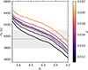 |
Fig. 8. Buoyancy travel time vs. central H fraction for a 1.5 M⊙ star, for various metallicities, using data from Mombarg et al. (2021). The buoyancy travel time for KIC 4150611 (see Sect. 4), which is an input for the MCMC grid-search component of the modelling, is shown as the horizontal grey band. The grey lines are the solar metallicity, rotating stellar models from Mombarg et al. (2024a) (grid B); the width of the band that they form is indicative of the variation due to stellar rotation. |
However, the treatment of mixing can also affect Π0 significantly; the solar metallicity models from Mombarg et al. (2024b) (grid C) have a similar Π0 profile to the Z = 0.011 profile in Fig. 8 (grid A), differing significantly from the solar metallicity models of Mombarg et al. (2024a) (grid B). This implies that internal physical choices can be as important as matching the metallicity when using Π0. The Z = 0.0045 (grid D) models from Mombarg et al. (2024b) have significantly lower values of Π0, as anticipated, but also a very flat Π0–Xc behaviour between Xc = 0.55 and Xc = 0.3, implying lower sensitivity to stellar ages in this region. This flattening is particularly pronounced for higher fov.
Considering now only the MCMC simulations where the input parameters were able to be recovered within uncertainty (grids A, C, and E), we find that the results are broadly consistent with the pattern modelling approach using C-3PO and consistent with each-other. We also note that, as we might expect, grid E – which most closely matches the metallicity of KIC 4150611 – does a slightly better job at recovering the input parameters.
From our MCMC modelling, we estimate KIC 4150611 to be a 1.52 ± 0.06 M⊙ star with Xc = 0.48 ± 0.08, values consistent with those found by our C-3PO modelling, albeit slightly higher in the case of Xc = 0.48 ± 0.08. This methodology was unable to constrain fov, likely due to this parameter being insufficiently constrained by Π0 alone. This was also the case in Fritzewski et al. (2024), and highlights the added value of pattern-modelling relative to parameter-based grid-search methods.
However, one advantage of the MCMC method is its ability to sample all evolutionary parameters accessible through the MCMC chain, giving access to stellar properties that cannot be directly accessed via C-3PO. We estimate the stellar age to be 1110 ± 150 Myr, in agreement with our previous estimates. Furthermore, we find a convective core mass fraction Mconv/M = 0.09 ± 0.01, which is consistent with the distribution of other Keplerγ Dor stars (Mombarg et al. 2019).
5. Conclusions
In this work we modelled the g-mode period-spacing pattern of the Aa component of KIC 4150611 with the goal of estimating its stellar parameters. This was done with attention to how the different external constraints from spectroscopy and photometric eclipse modelling interplay with the asteroseismic information. We also considered four different period-spacing patterns for the system to account for systematic differences in pattern identification and frequency extraction methods.
We find that pattern-dependent frequency variations are less important than the completeness of the pattern, particularly in terms of how far the pattern extends to high radial orders. For several key parameters, such as the stellar mass and core hydrogen fraction, there is a clear bifurcation between the parameter estimation from the shorter patterns, PAT_LI2020 and PAT_P04_PES, and the longer PAT_P04_OPT and PAT_STS patterns. The parameters for the longer PAT_P04_OPT and particularly the PAT_STS patterns agree best with external information from the eclipse modelling, spectroscopy, and the system luminosity calculated from Gaia DR3 data.
For patterns with a length and completeness similar to that of KIC 4150611, the pattern is unlikely to be constraining enough for confident conclusions to be drawn for many stellar parameters without the benefit of external constraints. Notable exceptions include near-core properties such as the degree of exponential overshoot and the near-core rotation. It also appears that the effective temperature can be consistently estimated from the seismology alone, likely due to it being correlated with the buoyancy travel time.
When the external spectroscopic and constraints are considered in isolation, they are generally uninformative for any given parameter. However, the intersection of their 2σ uncertainty regions does allow for useful – although imprecise – bounds to be placed on the mass, central hydrogen fraction, and luminosity. However, it is unhelpful when considering the metallicity, degree of core overshooting, and the near-core rotation.
We find the near-core rotation rate to be 1.58 ± 0.01 d−1, consistent with Li et al. (2020a). Combined with an estimate for the surface rotation frequency of 1.54 ± 0.10 d−1, this is consistent with a near-perfect rigid rotation of the radiative zone. We estimate the buoyancy travel time to be 4024 ± 74 s, also consistent with Li et al. (2020a).
By considering the spectroscopic and eclipse-modelling constraints in conjunction with asteroseismology, we arrive at the best motivated constraints of the stellar parameters. We estimate the stellar mass to be between 1.47 M⊙ and 1.51 M⊙ (±0.05 M⊙), preferring the high-mass solutions around 1.51 M⊙ from the PAT_P04_OPT and PAT_STS patterns. The core hydrogen fraction we find to be between 0.42 and 0.49 (±0.04). The lower values correspond to the preferred PAT_P04_OPT and PAT_LI2020 patterns; we also note that core hydrogen fractions no higher than 0.58 are permitted based on the intersecting radius and spectroscopic constraints. We find the stellar radii to be between 1.55 R⊙ and 1.68 R⊙ (with uncertainties no higher than ±0.1R⊙), preferring the higher radius solutions from the PAT_P04_OPT and PAT_STS patterns, which we note are more consistent with the eclipse modelling from Kemp et al. (2024). The metallicity shows, for all patterns and constraints, a preference for the lower metallicity bound of C-3PO. This is consistent with atmospheric modelling estimates for the metallicity from Kemp et al. (2024), which place the star slightly below the metallicity range able to be modelled by C-3PO. The best-fitting models consistently prefer low values of exponential overshooting regardless of the pattern or constraint considered. This is consistent with the low-mass end of the empirical M-fov relation for γ Dor stars put forth by Claret & Torres (2017), as well as the probability distributions for γ Dor stars computed by Mombarg et al. (2024a).
The best-fitting models have Teff between 7160 K and 7180 K, placing them just below the 1σ uncertainty region from the spectroscopic analysis (7280 ± 70 K). The uncertainty estimates for log(Teff) of approximately ±0.008 dex overlap with the spectroscopic solution. Helped considerably by the intersecting radius and spectroscopic constraints, the best-fitting models have log(g) values that vary between 4.168 dex and 4.223 dex (±0.04 dex), with the results from the preferred PAT_P04_OPT and PAT_LI2020 fits at the lower end of the range. We find that log(L), also helped considerably by the intersecting spectroscopic and radius constraints, is between 0.745 dex and 0.819 dex (±0.005 dex), preferring the high luminosity solutions from the PAT_P04_OPT and PAT_STS patterns. These higher solutions are consistent with the stellar luminosity calculated from Gaia DR3 and light fractions for Aa from Kemp et al. (2024) and Hełminiak et al. (2017).
We estimate the age of Aa to be approximately 1100 ± 100 Myr, much older than Hełminiak et al. (2017)’s 35 Myr age estimate from isochrone fitting. This older age from asteroseismology is also supported by the radius measurement from Kemp et al. (2024) and serves as a reminder of the important role that asteroseismology can play in stellar parameter estimation.
From our parameter-based MCMC grid search, we were able to recover similar solutions for the stellar parameters of KIC 4150611 Aa, including the stellar age. Comparing different model grids, the significant effect of metallicity on the buoyancy travel time was evident. The need for careful treatment of the envelope mixing was also evident as it potentially affects the buoyancy travel as much as the metallicity.
In future work it would be interesting to revisit the isochrone fitting of the B system in an attempt to confirm its age, ideally in parallel with an independent isochrone ageing of the components of the A triple system using their radii and estimated seismic masses. KIC 4150611 is not part of a particularly crowded field, so the fact that there are four sets of eclipses is highly suggestive of a physical association, and likely a co-evolutionary origin, between its A, B, and C components. A revisit of the ageing of different system components could provide clarity on this issue and greatly assist in establishing the evolution history of this fascinating system.
Data availability
Supplementary material can be found online https://zenodo.org/records/14275585. This material includes extra data and figures, as well as an online appendix. Technical data and figures are available upon request from the lead author (This email address is being protected from spambots. You need JavaScript enabled to view it. ).
HD 141469; RA = 19°18′58.21759″, Dec = +39°16′01.7913″ (J2000).
Gaia’s distance_gspphot label.
The bolometric correction is taken to be +0.01, see https://www.pas.rochester.edu/%7Eemamajek/EEM_dwarf_UBVIJHK_colors_Teff.txt (Pecaut & Mamajek 2013).
Equivalent to a 2D histogram but instead of colouring by the count, a pie chart that accounts for the relative number of qualitatively different data is drawn in each bin (here the different combinations of external constraints). Code for producing scatter pies can be found at: https://github.com/Alex162/scatterpie
In an additional online appendix, we discuss the possibility of a very short l = 2 series of g-modes.
The initial core hydrogen fraction is approximately 0.7, with the precise value depending on the metallicity.
Acknowledgments
The authors wish to thank Sarah Gebruers, Dominic Bowman, and Annachiara Picco for their useful discussion and input. The research leading to these results has received funding from the KU Leuven Research Council (grant C16/18/005: PARADISE), from the Research Foundation Flanders (FWO) under grant agreement G089422N (AT, CA) and 1124321N (LIJ), as well as from the BELgian federal Science Policy Office (BELSPO) through PRODEX grant PLATO. V.V. gratefully acknowledges support from the Research Foundation Flanders (FWO) under grant agreement N°1156923N (PhD Fellowship). JSGM acknowledges funding the French Agence Nationale de la Recherche (ANR), under grant MASSIF (ANR-21-CE31-0018-02). CA acknowledges funding by the European Research Council under grant ERC SyG 101071505. Funded by the European Union. Views and opinions expressed are however those of the author(s) only and do not necessarily reflect those of the European Union or the European Research Council. Neither the European Union nor the granting authority can be held responsible for them. This paper includes data collected by the Kepler mission, which are publicly available from the Mikulski Archive for Space Telescopes (MAST) at the Space Telescope Science Institute (STScI). Funding for the Kepler mission is provided by the NASA Science Mission Directorate. STScI is operated by the Association of Universities for Research in Astronomy, Inc., under NASA contract NAS 5-26555.
References
- Aerts, C. 2021, Rev. Mod. Phys., 93, 015001 [Google Scholar]
- Aerts, C., & Tkachenko, A. 2024, A&A, 692, R1 [NASA ADS] [CrossRef] [EDP Sciences] [Google Scholar]
- Aerts, C., Waelkens, C., Daszyńska-Daszkiewicz, J., et al. 2004, A&A, 415, 241 [NASA ADS] [CrossRef] [EDP Sciences] [Google Scholar]
- Aerts, C., Christensen-Dalsgaard, J., & Kurtz, D. W. 2010, Asteroseismology (Springer) [Google Scholar]
- Aerts, C., Molenberghs, G., Michielsen, M., et al. 2018, ApJS, 237, 15 [Google Scholar]
- Aerts, C., Van Reeth, T., Mombarg, J. S. G., & Hey, D. 2024, A&A, submitted [Google Scholar]
- Asplund, M., Grevesse, N., Sauval, A. J., & Scott, P. 2009, ARA&A, 47, 481 [NASA ADS] [CrossRef] [Google Scholar]
- Baglin, A. 2003, Adv. Space Res., 31, 345 [NASA ADS] [CrossRef] [Google Scholar]
- Balona, L. A. 2014, MNRAS, 443, 1946 [NASA ADS] [CrossRef] [Google Scholar]
- Baran, A. S., Koen, C., & Pokrzywka, B. 2015, MNRAS, 448, L16 [NASA ADS] [CrossRef] [Google Scholar]
- Berthomieu, G., Gonczi, G., Graff, P., Provost, J., & Rocca, A. 1978, A&A, 70, 597 [Google Scholar]
- Borucki, W. J., Koch, D., Basri, G., et al. 2010, Science, 327, 977 [Google Scholar]
- Bouabid, M. P., Dupret, M. A., Salmon, S., et al. 2013, MNRAS, 429, 2500 [Google Scholar]
- Claret, A., & Torres, G. 2017, ApJ, 849, 18 [Google Scholar]
- De Cat, P., & Aerts, C. 2002, A&A, 393, 965 [NASA ADS] [CrossRef] [EDP Sciences] [Google Scholar]
- De Cat, P., Eyer, L., Cuypers, J., et al. 2006, A&A, 449, 281 [NASA ADS] [CrossRef] [EDP Sciences] [Google Scholar]
- Degroote, P., Aerts, C., Ollivier, M., et al. 2009, A&A, 506, 471 [NASA ADS] [CrossRef] [EDP Sciences] [Google Scholar]
- Dupret, M. A., Grigahcène, A., Garrido, R., Gabriel, M., & Scuflaire, R. 2005, A&A, 435, 927 [NASA ADS] [CrossRef] [EDP Sciences] [Google Scholar]
- Eckart, C. 1960, Phys. Fluids, 3, 421 [Google Scholar]
- Freytag, B., Ludwig, H. G., & Steffen, M. 1996, A&A, 313, 497 [NASA ADS] [Google Scholar]
- Fritzewski, D. J., Aerts, C., Mombarg, J. S. G., Gossage, S., & Van Reeth, T. 2024, A&A, 684, A112 [NASA ADS] [CrossRef] [EDP Sciences] [Google Scholar]
- Gaia Collaboration (Prusti, T., et al.) 2016, A&A, 595, A1 [NASA ADS] [CrossRef] [EDP Sciences] [Google Scholar]
- Gaia Collaboration (Vallenari, A., et al.) 2023, A&A, 674, A1 [NASA ADS] [CrossRef] [EDP Sciences] [Google Scholar]
- Gebruers, S., Straumit, I., Tkachenko, A., et al. 2021, A&A, 650, A151 [NASA ADS] [CrossRef] [EDP Sciences] [Google Scholar]
- Hełminiak, K. G., Ukita, N., Kambe, E., et al. 2017, A&A, 602, A30 [NASA ADS] [CrossRef] [EDP Sciences] [Google Scholar]
- Herwig, F. 2000, A&A, 360, 952 [NASA ADS] [Google Scholar]
- Hough, S. S. 1898, Philos. Trans. R. Soc. London Ser. A, 191, 139 [NASA ADS] [CrossRef] [Google Scholar]
- IJspeert, L. W., Tkachenko, A., Johnston, C., et al. 2024, A&A, 685, A62 [NASA ADS] [CrossRef] [EDP Sciences] [Google Scholar]
- Johnson, R. A., Wichern, D. W., et al. 2019, Applied Multivariate Statistical Analysis (Prentice Hall) [Google Scholar]
- Johnston, C., Tkachenko, A., Aerts, C., et al. 2019, MNRAS, 482, 1231 [Google Scholar]
- Kemp, A., Tkachenko, A., Torres, G., et al. 2024, A&A, 689, A164 [NASA ADS] [CrossRef] [EDP Sciences] [Google Scholar]
- Lee, U., & Saio, H. 1989, MNRAS, 237, 875 [NASA ADS] [Google Scholar]
- Lee, U., & Saio, H. 1997, ApJ, 491, 839 [Google Scholar]
- Li, G., Van Reeth, T., Bedding, T. R., Murphy, S. J., & Antoci, V. 2019a, MNRAS, 487, 782 [Google Scholar]
- Li, G., Bedding, T. R., Murphy, S. J., et al. 2019b, MNRAS, 482, 1757 [Google Scholar]
- Li, G., Guo, Z., Fuller, J., et al. 2020a, MNRAS, 497, 4363 [Google Scholar]
- Li, G., Van Reeth, T., Bedding, T. R., et al. 2020b, MNRAS, 491, 3586 [Google Scholar]
- Li, G., Aerts, C., Bedding, T. R., et al. 2024, A&A, 686, A142 [NASA ADS] [CrossRef] [EDP Sciences] [Google Scholar]
- Lomb, N. R. 1976, Ap&SS, 39, 447 [Google Scholar]
- Mathis, S. 2009, A&A, 506, 811 [CrossRef] [EDP Sciences] [Google Scholar]
- Mathis, S., Talon, S., Pantillon, F. P., & Zahn, J. P. 2008, Sol. Phys., 251, 101 [NASA ADS] [CrossRef] [Google Scholar]
- Michielsen, M. 2024, J. Open Source Softw., 9, 5884 [NASA ADS] [CrossRef] [Google Scholar]
- Michielsen, M., Aerts, C., & Bowman, D. M. 2021, A&A, 650, A175 [NASA ADS] [CrossRef] [EDP Sciences] [Google Scholar]
- Michielsen, M., Van Reeth, T., Tkachenko, A., & Aerts, C. 2023, A&A, 679, A6 [NASA ADS] [CrossRef] [EDP Sciences] [Google Scholar]
- Miglio, A., Montalbán, J., Noels, A., & Eggenberger, P. 2008, MNRAS, 386, 1487 [Google Scholar]
- Mombarg, J. S. G., Van Reeth, T., Pedersen, M. G., et al. 2019, MNRAS, 485, 3248 [NASA ADS] [CrossRef] [Google Scholar]
- Mombarg, J. S. G., Van Reeth, T., & Aerts, C. 2021, A&A, 650, A58 [NASA ADS] [CrossRef] [EDP Sciences] [Google Scholar]
- Mombarg, J. S. G., Aerts, C., & Molenberghs, G. 2024a, A&A, 685, A21 [NASA ADS] [CrossRef] [EDP Sciences] [Google Scholar]
- Mombarg, J. S. G., Aerts, C., Van Reeth, T., & Hey, D. 2024b, A&A, 691, A131 [NASA ADS] [CrossRef] [EDP Sciences] [Google Scholar]
- Niemczura, E., Murphy, S. J., Smalley, B., et al. 2015, MNRAS, 450, 2764 [Google Scholar]
- Ogilvie, G. I., & Lin, D. N. C. 2004, ApJ, 610, 477 [Google Scholar]
- Paxton, B., Cantiello, M., Arras, P., et al. 2013, ApJS, 208, 4 [Google Scholar]
- Pecaut, M. J., & Mamajek, E. E. 2013, ApJS, 208, 9 [Google Scholar]
- Pedersen, M. G., Aerts, C., Pápics, P. I., et al. 2021, Nat. Astron., 5, 715 [NASA ADS] [CrossRef] [Google Scholar]
- Prša, A., Batalha, N., Slawson, R. W., et al. 2011, AJ, 141, 83 [Google Scholar]
- Ricker, G. R., Winn, J. N., Vanderspek, R., et al. 2015, J. Astron. Telesc. Instrum. Syst., 1, 014003 [Google Scholar]
- Rowe, J. F., Coughlin, J. L., Antoci, V., et al. 2015, ApJS, 217, 16 [NASA ADS] [CrossRef] [Google Scholar]
- Scargle, J. D. 1982, ApJ, 263, 835 [Google Scholar]
- Schmid, V. S., & Aerts, C. 2016, A&A, 592, A116 [NASA ADS] [CrossRef] [EDP Sciences] [Google Scholar]
- Shaviv, G., & Salpeter, E. E. 1973, ApJ, 184, 191 [Google Scholar]
- Shibahashi, H. 1979, PASJ, 31, 87 [NASA ADS] [Google Scholar]
- Shibahashi, H., & Kurtz, D. W. 2012, MNRAS, 422, 738 [Google Scholar]
- Szentgyorgyi, A. H., & Furész, G. 2007, Rev. Mex. Astron. Astrofis. Conf. Ser., 28, 129 [NASA ADS] [Google Scholar]
- Tassoul, M. 1980, ApJS, 43, 469 [Google Scholar]
- Tkachenko, A. 2015, A&A, 581, A129 [NASA ADS] [CrossRef] [EDP Sciences] [Google Scholar]
- Townsend, R. H. D. 2020, MNRAS, 497, 2670 [NASA ADS] [CrossRef] [Google Scholar]
- Townsend, R. H. D., & Teitler, S. A. 2013, MNRAS, 435, 3406 [Google Scholar]
- Triana, S. A., Moravveji, E., Pápics, P. I., et al. 2015, ApJ, 810, 16 [Google Scholar]
- Uytterhoeven, K., Moya, A., Grigahcène, A., et al. 2011, A&A, 534, A125 [CrossRef] [EDP Sciences] [Google Scholar]
- Van Beeck, J., Bowman, D. M., Pedersen, M. G., et al. 2021, A&A, 655, A59 [NASA ADS] [CrossRef] [EDP Sciences] [Google Scholar]
- Van Reeth, T., Tkachenko, A., Aerts, C., et al. 2015a, A&A, 574, A17 [NASA ADS] [CrossRef] [EDP Sciences] [Google Scholar]
- Van Reeth, T., Tkachenko, A., Aerts, C., et al. 2015b, ApJS, 218, 27 [Google Scholar]
- Van Reeth, T., Tkachenko, A., & Aerts, C. 2016, A&A, 593, A120 [NASA ADS] [CrossRef] [EDP Sciences] [Google Scholar]
- Van Reeth, T., Mombarg, J. S. G., Mathis, S., et al. 2018, A&A, 618, A24 [NASA ADS] [EDP Sciences] [Google Scholar]
- Van Reeth, T., De Cat, P., Van Beeck, J., et al. 2022, A&A, 662, A58 [NASA ADS] [CrossRef] [EDP Sciences] [Google Scholar]
- Van Reeth, T., Johnston, C., Southworth, J., et al. 2023, A&A, 671, A121 [NASA ADS] [CrossRef] [EDP Sciences] [Google Scholar]
- Zahn, J. P. 1991, A&A, 252, 179 [Google Scholar]
Appendix A: Detailed period-spacing pattern plots
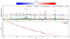 |
Fig. A.1. PAT_LI2020 period-spacing pattern from Li et al. (2020a). The Lomb-Scargle periodogram is shown in grey, the extracted frequencies in light blue, and the residual periodogram with the extracted frequencies removed in orange. Orbital harmonics are excluded. The S/N is indicated by the colour of the ‘X’ symbol for each extracted frequency, while the amplitude and period errors (more easily seen in the inset panel, which better shows the low-amplitude behaviour) are shown in orange. The extracted frequencies selected to be part of the pattern are marked with a filled black circle. Note that only the black point and the AMiGO fit and predictions are specifically related to the PAT_LI2020 pattern; the Lomb-Scargle periodogram and its residuals, as well as the extracted frequencies (and their associated S/N and errors), are included from the period04 extraction for comparison purposes. |
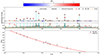 |
Fig. A.2. PAT_P04_PES period-spacing pattern. Orbital harmonics are excluded. The high-amplitude period at 0.36d is excluded in this pattern only due to its near-perfect coincidence with an 8.65d orbital harmonic. A detailed description of all symbols and information can be found in Fig. A.1. |
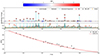 |
Fig. A.3. PAT_P04_OPT period-spacing pattern. Orbital harmonics are excluded. A detailed description of all symbols and information can be found in Fig. A.1. |
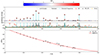 |
Fig. A.4. PAT_STS period-spacing pattern. Orbital harmonics are excluded. A detailed description of all symbols and information can be found in Fig. A.1. |
Appendix B: C-3PO modelling results
Parameters of the best-fitting models from C-3PO’s high resolution sample for each pattern under different external constraints.
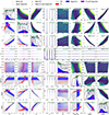 |
Fig. B.1. PAT_LI2020 modelling results. The main diagonal (emphasised with thicker panel outlines) shows the 1/χ2 envelopes (the maximum value of 1/χ2 per bin; solid lines) and histograms of the 1/χ2 values for each variable along the x-axis when considering purely the asteroseismic fit (All; grey), when only considering models that fall within spectroscopic constraints on log(g) and Teff (Spectro; blue), and when considering only models that satisfy both the spectroscopic constraints and constraints on the stellar radius from eclipse modelling (R and Spectro; purple). Best-fitting models are shown for each case. The green markers indicate the 100 best-fitting models. The lower triangular panels are ‘scatter pies’ (see the main text) showing how the different external constraints intersect along each 2D projection of the parameter space, with the best-fitting models also shown. The upper triangular panels show the maximum value of 1/χ2 for each 2D bin (logarithmic scale, with dark colouration indicating a better fit). |
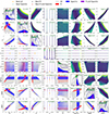 |
Fig. B.2. PAT_P04_PES modelling results. |
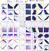 |
Fig. B.3. PAT_P04_OPT modelling results |
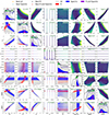 |
Fig. B.4. PAT_STS modelling results. |
All Tables
Parameters of the best-fitting models from C-3PO’s high resolution sample for each pattern under different external constraints.
All Figures
|
Fig. 1. System hierarchy and nomenclature of KIC 4150611, with approximate orbital periods shown in days. Hełminiak et al. (2017) present astrometric evidence for an association between the A and B components, but otherwise the A, B, and C components can be considered dynamically independent. The figure is based on Fig. 15 from Hełminiak et al. (2017). |
| In the text | |
|
Fig. 2. 4-year time series for KIC 4150611. Bottom: Normalised, detrended light curve (black; excluding the 94.2 d eclipses) and the sinusoid model (red) formed from all frequencies extracted using STAR SHADOW. Top: Residuals (blue). Figure 1 of Kemp et al. (2024) shows the equivalent figure for the extracted sinusoid model extracted using period04. |
| In the text | |
|
Fig. 3. Phase-folded light curves for each of the eclipsing components and its sinusoid model. The light curve (grey data) for each is the residual between the normalised, detrended light curve and every frequency except those forming the sinusoid model of the relevant eclipse from STAR SHADOW. The median flux is shown in green, and the coloured points (colour varies by panel) are from the relevant harmonic model. Figure 3 of Kemp et al. (2024) shows the equivalent figure for the period04 extraction, with no significant eclipse geometry differences. |
| In the text | |
|
Fig. 4. Lomb-Scargle periodogram of the normalised, detrended light curve (grey) with non-orbital harmonic frequencies extracted by STAR SHADOW (light blue) and the periodogram of the residual light curve (orange). The lower panel is the periodogram of the light curve when the orbital harmonics (see Fig. 3) are removed. |
| In the text | |
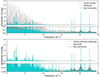 |
Fig. 5. Same as Fig. 4 but showing the period04 frequency extraction. |
| In the text | |
|
Fig. 6. Period-spacing patterns considered in this work, along with their AMiGO fits. |
| In the text | |
|
Fig. 7. Best-fitting C-3PO models (red) consistent with the radial and spectroscopic constraints (see Table B.1): PAT_LI2020 (a), PAT_P04_PES (b), PAT_P04_OPT (c), and PAT_STS (d). Observed patterns are shown in black. |
| In the text | |
|
Fig. 8. Buoyancy travel time vs. central H fraction for a 1.5 M⊙ star, for various metallicities, using data from Mombarg et al. (2021). The buoyancy travel time for KIC 4150611 (see Sect. 4), which is an input for the MCMC grid-search component of the modelling, is shown as the horizontal grey band. The grey lines are the solar metallicity, rotating stellar models from Mombarg et al. (2024a) (grid B); the width of the band that they form is indicative of the variation due to stellar rotation. |
| In the text | |
|
Fig. A.1. PAT_LI2020 period-spacing pattern from Li et al. (2020a). The Lomb-Scargle periodogram is shown in grey, the extracted frequencies in light blue, and the residual periodogram with the extracted frequencies removed in orange. Orbital harmonics are excluded. The S/N is indicated by the colour of the ‘X’ symbol for each extracted frequency, while the amplitude and period errors (more easily seen in the inset panel, which better shows the low-amplitude behaviour) are shown in orange. The extracted frequencies selected to be part of the pattern are marked with a filled black circle. Note that only the black point and the AMiGO fit and predictions are specifically related to the PAT_LI2020 pattern; the Lomb-Scargle periodogram and its residuals, as well as the extracted frequencies (and their associated S/N and errors), are included from the period04 extraction for comparison purposes. |
| In the text | |
|
Fig. A.2. PAT_P04_PES period-spacing pattern. Orbital harmonics are excluded. The high-amplitude period at 0.36d is excluded in this pattern only due to its near-perfect coincidence with an 8.65d orbital harmonic. A detailed description of all symbols and information can be found in Fig. A.1. |
| In the text | |
|
Fig. A.3. PAT_P04_OPT period-spacing pattern. Orbital harmonics are excluded. A detailed description of all symbols and information can be found in Fig. A.1. |
| In the text | |
|
Fig. A.4. PAT_STS period-spacing pattern. Orbital harmonics are excluded. A detailed description of all symbols and information can be found in Fig. A.1. |
| In the text | |
|
Fig. B.1. PAT_LI2020 modelling results. The main diagonal (emphasised with thicker panel outlines) shows the 1/χ2 envelopes (the maximum value of 1/χ2 per bin; solid lines) and histograms of the 1/χ2 values for each variable along the x-axis when considering purely the asteroseismic fit (All; grey), when only considering models that fall within spectroscopic constraints on log(g) and Teff (Spectro; blue), and when considering only models that satisfy both the spectroscopic constraints and constraints on the stellar radius from eclipse modelling (R and Spectro; purple). Best-fitting models are shown for each case. The green markers indicate the 100 best-fitting models. The lower triangular panels are ‘scatter pies’ (see the main text) showing how the different external constraints intersect along each 2D projection of the parameter space, with the best-fitting models also shown. The upper triangular panels show the maximum value of 1/χ2 for each 2D bin (logarithmic scale, with dark colouration indicating a better fit). |
| In the text | |
|
Fig. B.2. PAT_P04_PES modelling results. |
| In the text | |
|
Fig. B.3. PAT_P04_OPT modelling results |
| In the text | |
|
Fig. B.4. PAT_STS modelling results. |
| In the text | |
Current usage metrics show cumulative count of Article Views (full-text article views including HTML views, PDF and ePub downloads, according to the available data) and Abstracts Views on Vision4Press platform.
Data correspond to usage on the plateform after 2015. The current usage metrics is available 48-96 hours after online publication and is updated daily on week days.
Initial download of the metrics may take a while.