| Issue |
A&A
Volume 693, January 2025
|
|
|---|---|---|
| Article Number | A7 | |
| Number of page(s) | 15 | |
| Section | Planets, planetary systems, and small bodies | |
| DOI | https://doi.org/10.1051/0004-6361/202451859 | |
| Published online | 23 December 2024 | |
The GAPS programme at TNG
LXIV. An inner eccentric sub-Neptune and an outer sub-Neptune-mass candidate around BD+00 444 (TOI-2443)
1
INAF – Osservatorio Astrofisico di Torino,
Via Osservatorio 20,
10025
Pino Torinese,
Italy
2
Dipartimento di Fisica, Università degli studi di Roma “Tor Vergata”,
Rome,
Italy
3
Max-Planck-Institut für Astronomie,
Heidelberg,
Germany
4
Institute for Particle Physics and Astrophysics, ETH Zürich,
Otto-Stern-Weg 5,
8093
Zürich,
Switzerland
5
INAF – Osservatorio Astronomico di Roma,
Monte Porzio Catone,
Italy
6
INAF – Osservatorio Astrofisico di Catania,
Via S. Sofia 78,
95123
Catania,
Italy
7
INAF – Osservatorio Astronomico di Padova,
Padova,
Italy
8
Center for Astrophysics | Harvard & Smithsonian,
60 Garden Street,
Cambridge,
MA
02138,
USA
9
George Mason University,
4400 University Drive,
Fairfax,
VA,
22030
USA
10
INAF – Osservatorio Astronomico di Palermo,
Piazza del Parlamento 1,
90134
Palermo,
Italy
11
Dipartimento di Fisica e Chimica “Emilio Segrè”, Università di Palermo,
Via Archirafi 36,
Palermo,
Italy
12
Observatoire de Genéve, Université de Genéve,
1290
Versoix,
Switzerland
13
INAF – Fundación Galileo Galilei,
Rambla J. A. F. Pérez 7,
38712
Breña Baja,
TF,
Spain
14
Instituto de Astrofísica de Canarias (IAC),
c/ Vía Láctea s/n,
38205,
La Laguna (Tenerife),
Canary Islands,
Spain
15
Dipartimento di Fisica e Astronomia “Galileo Galilei”,
Vicolo dell’Osservatorio 3,
35122
Padova,
Italy
★ Corresponding author; This email address is being protected from spambots. You need JavaScript enabled to view it.
Received:
11
August
2024
Accepted:
13
November
2024
Abstract
Context. Super-Earths and sub-Neptunes are the most common types of planets outside the Solar System and likely represent the link between terrestrial planets and gas giants. Characterizing their physical and orbital properties and studying their multiplicity are key steps in testing and understanding their formation, migration, and evolution.
Aims. We examined the star BD+00 444 (GJ 105.5, TOI-2443; V = 9.5 mag; d = 23.9 pc) in depth, with the aim of characterizing and confirming the planetary nature of its small companion, the planet candidate TOI-2443.01, which was discovered by the TESS space telescope and subsequently validated by a follow-up statistical study.
Methods. We monitored BD+00 444 with the HARPS-N spectrograph for 1.5 years to search for planet-induced radial-velocity (RV) variations, and then analyzed the RV measurements jointly with TESS and ground-based photometry.
Results. We determined that the host is a quiet K5 V star with a radius of R* = 0.631−0.014+0.013 R⊕ and a mass of M* = 0.642−0.025+0.026 M⊙. We revealed that the sub-Neptune BD+00 444 b has a radius of Rb = 2.36 ± 0.05 R⊕, a mass of Mb = 4.8 ± 1.1 M⊕, and consequently a rather low-density value of ρb = 2.00−0.45+0.49 g cm−3, which makes it compatible with both an Earth-like rocky interior with a thin H-He atmosphere and a half-rocky, half-water composition with a small amount of H-He. With an orbital period of about 15.67 days and an equilibrium temperature of about 519 K, BD+00 444 b has an estimated transmission spectroscopy metric (TSM) of 159−31+46, which makes it ideal for atmospheric follow-up with the James Webb Space Telescope. Notably, it is the second most eccentric inner transiting planet among those with well-determined eccentricities, with e = 0.302−0.035+0.051, and a mass of below 20 M⊕. We estimated that tidal forces from the host star affect both the rotation and eccentricity of planet b, and strong tidal dissipation may signal intense volcanic activity. Furthermore, our analysis suggests the presence of a sub-Neptune-mass planet candidate, BD+00 444 c, which would have an orbital period of Pc = 96.6 ± 1.4 days and a minimum mass of Mc sin i = 9.3−2.0+1.8 M⊕. With an equilibrium temperature of about 283 K, BD+00 444 c is inside the habitable zone; however, confirmation of this candidate would require further observations and stronger statistical evidence. We explored the formation and migration of both planets by means of population synthesis models, which reveal that both planets started their formation beyond the water snowline during the earliest phases of the life of their protoplanetary disk.
Key words: instrumentation: photometers / instrumentation: spectrographs / methods: data analysis / techniques: photometric / techniques: radial velocities / occultations
© The Authors 2024
 Open Access article, published by EDP Sciences, under the terms of the Creative Commons Attribution License (https://creativecommons.org/licenses/by/4.0), which permits unrestricted use, distribution, and reproduction in any medium, provided the original work is properly cited.
This article is published in open access under the Subscribe to Open model. This email address is being protected from spambots. You need JavaScript enabled to view it. to support open access publication.
1 Introduction
One of the main findings of the NASA Kepler mission (Borucki et al. 2010) is that, in our Galaxy, small planets (Rp < 4 R⊕) at short orbital periods (Porb < 100 days) are the most common type (see, e.g., Bean et al. 2021; Biazzo et al. 2022a for recent and comprehensive reviews). Small planets with 1R⊕ < Rp < 4 R⊕ are thought to bridge the gap between the rocky, terrestrial planets and gas giants, even though they may have very large masses, as in the ultra-dense K2-292 b (M ≈ 25 M⊕; Luque et al. 2019). Kepler also revealed a deficit in the occurrence rate distribution at 1.5–2.0 R⊕, which is associated with a bimodality in their radius distribution (Fulton et al. 2017) that probably depends on whether or not their rocky cores have been able to retain a substantial hydrogen-rich envelope. This dichotomy has now become the classical way to a further subclassification into super-Earths and sub-Neptunes. At the same time, statistical studies of the orbital eccentricity of transiting planets with Rp < 6 R⊕ tell us that single transiting planets display higher average eccentricities than transiting planets in multiple systems, possibly reflecting differences in their formation pathways (Van Eylen & Albrecht 2015; Xie et al. 2016). Numerical simulations show that massive external companions in multi-planet systems containing sub-Neptunes may perturb their orbits by exciting their eccentricity, producing wider spacing and increasing the mutual inclination among planets (Pu & Lai 2018), thus making it more unlikely to observe multiple transiting planets. This result can explain why systems with fewer transiting planets are dynamically hotter (i.e., they are more eccentric and inclined) than those with a greater number of transiting planets, although this excitation can also be self-induced in tightly packed systems (Van Eylen et al. 2019).
Currently, with TESS (Ricker et al. 2014) continuously scanning the skies, a large number of new sub-Neptune exoplanets are being discovered (see, e.g., Badenas-Agusti et al. 2020; Cointepas et al. 2021; Burt et al. 2021; Gan et al. 2022; Kiefer et al. 2023; Suárez Mascareño et al. 2024; Montalto et al. 2024). Characterizing these planets is essential if we are to enhance our understanding of this class of exoplanets, particularly those that are favorable targets for atmospheric studies with the JWST. Indeed, observational constraints on sub-Neptune atmospheres can provide information about their compositions, though their atmospheric chemistry is still largely unknown given the technical difficulty in probing them (e.g., Kreidberg et al. 2014; Tsiaras et al. 2016; Mikal-Evans et al. 2023). However, thanks to JWST, which began operations in July 2022, we have entered a new era of atmospheric characterization (JWST Transiting Exoplanet Community Early Release Science Team 2023). The first investigations of sub-Neptune atmospheres have already been performed, such as those of K2-18 b (Madhusudhan et al. 2023) and TOI-270 d (Holmberg & Madhusudhan 2024), although the interpretation of these transmission spectra raised some controversy (e.g., Wogan et al. 2024). A large observational program is currently underway to investigate the atmospheric presence and composition of a dozen super-Earth and sub-Neptune exoplanets (i.e., Compositions of Mini-Planet Atmospheres for Statistical Study, COMPASS; Wallack et al. 2024).
On 6 January 2021, the TESS target star TIC 318753380 (BD+00 444, GJ 105.5) was officially named TOI-2443 (TESS Object of Interest; Guerrero et al. 2021), following the summary of the data validation report (DVR) produced by the TESS Science Processing Operations Center (SPOC) (Jenkins et al. 2016) pipeline at the NASA Ames Research Center through the Transiting Planet Search (TPS; Jenkins 2002; Jenkins et al. 2010, 2020) and data validation (Twicken et al. 2018, Li et al. 2019) modules. In particular, as stated in this report, the difference image centroid locates the source of the transits within 4 arcsec of the target star’s location. The candidate TOI-2443.01 was designated as planet TOI-2443 b after the statistical validation of Mistry et al. (2023), in which the false-positive probability was evaluated using the TRICERATOPS tool (Giacalone et al. 2021). However, in the present work, we use the star’s original designation and refer to the planet as BD+00 444 b.
Within the Global Architecture of Planetary Systems (GAPS) Neptune project (Naponiello et al. 2022, 2023; Damasso et al. 2023), we started monitoring this target in July 2021 as the potential host of a sub-Neptune exoplanet. In particular, we took Doppler measurements with the High Accuracy Radial velocity Planet Searcher for the Northern hemisphere (HARPS-N; Cosentino et al. 2012) instrument installed at the Telescopio Nazionale Galileo (TNG) in La Palma (Spain). Here, we report the results of our observations and analyses, which allowed us to measure the mass of BD+00 444 b and discover a new candidate planet in the system. In particular, BD+00 444 b emerged as the second most eccentric inner transiting planet with a mass below 20M⊕ among those with eccentricities determined with at least 5σ accuracy, after the recently discovered TOI-757 b (Alqasim et al. 2024), and is the only one with a possible companion in the habitable zone (Sect. 5.1).
This paper is organized as follows. Section 2 contains the details of the photometric and RV observations. The star characterization is detailed in Sect. 3, while the analysis of the planetary signals is presented in Sect. 4 and discussed in Sect. 5. Finally, we draw our conclusions in Sect. 6.
2 Observations and data reduction
2.1 TESS photometry
The pre-selected target BD+00 444, located at about 23.9 pc, was shortly observed by TESS in Sector 31, between 21 October and 19 November 2020, and only two transit events were recorded. The two-minute cadence photometry of BD+00 444 from TESS spans about 25 days, with a gap of about 4 days in between, and was analyzed with the Python wrapper juliet1 (Espinoza et al. 2019) (as detailed in Sect. 4.2). In particular, we used the Presearch Data Conditioning Simple Aperture Photometry (PDC-SAP; Stumpe et al. 2012, 2014, Smith et al. 2012) light curve, which is provided by TESS SPOC pipeline and retrieved via the Python package lightkurve (Lightkurve Collaboration 2018) from the Mikulski Archive for Space Telescopes. The PDC-SAP photometry is already corrected for dilution from other objects contained within the aperture using the Create Optimal Apertures module (Bryson et al. 2010, 2020). In this case there are only two sources close to the borders of the SPOC aperture, within a 5–6 mag difference, as shown in Fig. 1 using tpfplotter2 (Aller et al. 2020). The PDC-SAP light curve is plotted, along with the two transits, in Fig. 2.
2.2 LCOGT light-curve follow up
Two near-full transits of BD+00 444 b were observed from two sites of the Las Cumbres Observatory Global Telescope (LCOGT; Brown et al. 2013) 1 m network. The first transit was observed on 19 September 2021 in the Pan-STARRS Y band (λc = 10 040 Å, Δλ = 1120 Å) from the Siding Spring Observatory near Coonabarabran, Australia. The second transit was observed on 10 September 2023 in Pan-STARRS zs band (λc = 8700 Å, Δλ = 1040 Å) from the McDonald Observatory near Fort Davis, Texas, USA. The LCOGT telescopes are equipped with a 4096 × 4096 SINISTRO camera having an image scale of 0″. 389 per pixel, resulting in a 26′ × 26′ field of view, and the images were calibrated using the standard LCOGT BANZAI pipeline (McCully et al. 2018), while differential photometric data were extracted using AstroImageJ (Collins et al. 2017). We used circular photometric apertures with radii 5″.0-7″.8 that excluded all the flux from the nearest known neighbors in the Gaia DR3 catalog (Fig. 1). The light curve data are available on the EXOFOP-TESS website3 and are included in the global modeling described in Sect. 4.2.
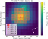 |
Fig. 1 Target pixel file from the TESS observation of Sector 31, centered on BD+00 444, which is marked with a white cross. The SPOC pipeline aperture is shown by shaded red squares, and the Gaia satellite DR3 catalog (Gaia Collaboration 2023) is also overlaid with symbol sizes proportional to the Gaia magnitude difference with BD+00 444. |
2.3 HARPS-N high-resolution spectra
Between 18 July 2021 and 18 January 2023, we collected a total of 97 high-resolution spectra of BD+00 444 with HARPS-N (Sect. 6) with a variable exposure time of 15–20 min. The RVs and activity indices were extracted from the spectra reduced using version 3.0.1 of the HARPS-N Data Reduction Software (DRS, Dumusque et al. 2021), available on the Data Analysis Center for Exoplanets (DACE) web platform. In the following analysis, we employed all the RVs, including a few with relatively lower signal-to-noise ratio (S/N), as their removal did not influence the results. Overall, the measurements have an average error of 1.6 m s-−1, a root mean square error of 3.3 m s−1, and an S/N ≈ 70, measured at a reference wavelength of 5500 Å.
3 Host-star characterization
3.1 Stellar parameters
A co-added spectrum was produced to derive stellar atmospheric parameters (effective temperature Teff, surface gravity log g⋆, micro-turbulence velocity ξ, and iron abundance [Fe/H]) through the MOOG code (Sneden 1973, version 2019) and adopting the MARCS atmospheric models (Gustafsson et al. 2008).
Similar results were obtained using the ATLAS9 grid of model atmospheres with new opacities (Castelli & Kurucz 2003). We adopted the list of Fe I and Fe II lines by Biazzo et al. (2022b) and imposed the condition that the Fe I abundance does not depend on the excitation potential and equivalent width of the lines for deriving Teff and ξ, respectively, and the Fe I/Fe II ionization equilibrium for determining log g. Our spectroscopic analysis provides as the final atmospheric parameters those listed in Table 1, in particular: Teff = 4375 ± 65 K, log g⋆ = 4.42 ± 0.20 cgs, ξ = 0.35 ± 0.35 km s−1, and [Fe/H]= −0.29 ± 0.12 dex.
We also estimated the effective temperature considering Gaia DR3 (Gaia Collaboration 2016, 2023) and 2MASS photometry (Skrutskie et al. 2006) and using the colte tool (Casagrande et al. 2021) with reddening taken from Capitanio et al. (2017). The total extinction coefficient, AV, is consistent with zero, as expected from a star at only about 24 pc.
The final weighted average of the photometric Teff from 12 colors is 4376 ± 81 K, in excellent agreement with our spectroscopic result. The stellar projected rotational velocity (υ sin i) was obtained through the 2009 version of the MOOG code (Sneden 1973) and the spectral-synthesis technique of three regions around 5400, 6200, and 6700 Å (Biazzo et al. 2022b). By assuming a macroturbolence velocity (Brewer et al. 2016) υmacro = 1.4 km s−1, we found υ sin i = 1.7 ± 0.8 km s−1, which is basically at the HARPS-N resolution limit, thus suggesting an inactive, slowly rotating star (see also Sect. 3.2), unless it is observed nearly pole-on.
We determined the stellar physical parameters, namely mass, radius, and age, with a Bayesian differential evolution Markov chain Monte Carlo framework through the EXOFASTv2 tool (Eastman 2017). Specifically, we performed simultaneous modeling of the stellar spectral energy distribution (SED) and the MESA Isochrones and Stellar Tracks (MIST, Paxton et al. 2015) by maximizing a combined Gaussian likelihood function given by the product of the SED and the MIST likelihoods (see Eastman et al. 2019 for more details). We sampled the SED with the Tycho-2 BT and VT, 2MASS J, H, and Ks, and WISE W1, W2, W3, and W4 magnitudes (see Table 1)4; we modeled it with the NexGen stellar atmospheric models (Allard et al. 2012) by varying Teff, log ɡ★, [Fe/H], the ratio of the stellar radius to the distance (R★/d), and the V-band extinction AV. Two additional free parameters for the MIST stellar models, properly interpolated by EXOFASTv2, are the stellar mass (M★) and age. We made use of previous information by imposing Gaussian priors on the Teff and [Fe/H] as derived from the spectral analysis as well as on the Gaia DR3 parallax. The fitted and derived (e.g., stellar luminosity and density) parameters of the host star are given in Table 1. Our stellar parameters supersede a number of previous determinations in the literature (e.g., Mishenina et al. 2008; Yee et al. 2017).
Stellar parameters of BD+00 444.
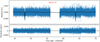 |
Fig. 2 Light curve of BD+00 444 as collected by TESS in Sector 31 with a two-minute cadence. Top panel: light curve from the PDC-SAP pipeline. The black line represents our best-fit transit model (from Sect. 4.2). Bottom panel: residuals of the best-fit model in parts per million. |
3.2 Stellar age indicators
We can estimate the age of our target using its rotation period (gyro-chronology), its chromospheric activity, or its spatial velocity components. The modulation of chromospheric lines might suggest a rotation period of about 45 d (Sect. 4.1) that can be used with the rotational isochrones of Barnes et al. (2016) assuming a Johnson B – V color of 1.20 mag (Koen et al. 2010).
The precision in stellar age is limited by the dispersion in the relationship between rotation, age, and color index. Additionally, the subsolar metallicity of our target is expected to reduce magnetic braking efficiency (Amard et al. 2020). Therefore, its true age can be older than estimated from the above standard gyro-chronological relationship.
The chromospheric activity index of BD+00 444, log R′HK, is equal to −5.004 ± 0.006, and it can be used to estimate old stellar ages according to Mamajek & Hillenbrand (2008). Given the sub-solar metallicity of our star, its chromospheric index is also expected to be enhanced at a given age with respect to a star with solar metallicity (Rocha-Pinto & Maciel 1998). The log R′HK was extracted from the DACE web interface5, and is computed from the S -index following Noyes et al. (1984). The S -index was derived by extracting the emission in the center of the Ca II H and K lines from order-merged spectra using a triangular band-pass normalized by two pseudo-continua on the blue and red-side of the two spectral lines, as defined by Vaughan et al. (1978). The corresponding log R′HK derived is therefore compatible with the original Mount-Wilson survey measurements (Wilson 1978).
We computed the Galactic velocity components of BD+00 444 with respect to the Sun (Table 1) using the method of Johnson & Soderblom (1987) as implemented in the IDL Astrolib procedure gal_uvw.pro. Adopting the UVW method of Almeida-Fernandes & Rocha-Pinto (2018), we estimated a kinematical age of 7.8 Gyr with a typical uncertainty of at least 3.0 Gyr, consistent with the age estimation from the stellar evolutionary tracks (cf. Table 1). Nevertheless, we reiterate the fact that kinematically based ages are highly uncertain for single stars because it is possible to find stars with an age of 1–3 Gyr having U, V, W velocity components typical of stars with ages of the order of 7–10 Gyr. In other words, the kinematical age is merely suggestive for a single star and provides a statistically meaningful indication only for a sufficiently large sample of coeval stars without kinematic peculiarities.
In conclusion, all the indirect methods considered above indicate that BD+00 444 is likely to be older than the Sun, although with a large uncertainty that makes its true age fall between about 1–2 and 10 Gyr.
3.3 Stellar companions
The high-contrast follow-up detailed by Mistry et al. (2023), including speckle imaging techniques with high-resolution observations, did not reveal the presence of any stellar companion. Similarly, despite possible offsets between the different instruments, we did not find significant long-term RV variations between the average RV from the HARPS-N orbital solution (Sect. 4) and previous measurements:  m s−1 from HARPS-N (N=97 measurements between 2021 and 2023), 72 930 ± 130 m s−1 from Gaia DR3 (2014–2017), 72 926 ± 3 m s−1 from SOPHIE (Perruchot et al. 2008) (N=1, 2011), 72 760 ± 50 m s−1 from ELODIE (Baranne et al. 1996)(N=3, 2000–2005). The Gaia DR3 archive also shows no co-moving objects within 900″ or ~20 000 au (i.e., no star with comparable parallax or proper motion). In the HIPPARCOS-Gaia astrometric acceleration (also known as proper motion anomaly, PMA) catalogs (Brandt 2021; Kervella et al. 2022), BD+00 444 was reported with no statistically significant indication of binarity, placing rather stringent constraints on the presence of low-mass giant planets (~50 M⊕) in the 3–10 au separation regime. However, BD+00 444 in the Gaia DR3 archive is reported to have a Renormalized Unit Weight Error (RUWE) of 1.25. This diagnostic is typically used to identify departures from a satisfactory single-star fit that might indicate the presence of orbital motion in Gaia DR3 astrometry (e.g., Lindegren et al. 2021), with a RUWE threshold of 1.4 usually adopted to discriminate the two categories. For nearby (ϖ > 35 mas), bright (G < 12 mag) stars with Gaia color in the range 1 mag < BP – RP < 2 mag as is the case for BD+00444, the typical RUWE is close to 1.0 (Sozzetti 2023). In principle, the presence of a giant planetary companion orbiting BD+00 444 at 1–3 au might help explain the (mild) departure from RUWE = 1.0 for the star, as in this range of orbital separations the PMA technique begins to lose sensitivity due to the smearing effect of the orbital motion for periods comparable to or shorter than the duration of the HIPPARCOS and Gaia DR3 observations. However, as shown later on in Section 4.3, a gas giant at such orbital distances should have been readily spotted based on the HARPS-N RV data at hand, unless it were to lie on a low inclination orbit (a detailed investigation of such a scenario from a dynamical stability standpoint is beyond the scope of this paper). A possible alternative explanation for the moderately elevated RUWE is instead due to larger unmodeled systematics in the astrometric time series.
4 Analysis
4.1 Periodograms of RV and photometric time series
We computed the Generalized Lomb-Scargle (GLS; Zechmeister & Kürster 2009) periodogram of the HARPS-N RVs, using the Python package astropy v.5.2.2 (Astropy Collaboration 2018). The orbital period of BD+00 444b, about 15.67 days, is rapidly spotted in the GLS, and it also corresponds to the primary peak of the maximum likelihood periodogram (MLP; Stoica et al. 1989), estimated with exostriker v.0.77 (Trifonov 2019) (top row of Fig. 3). Along with the expected signal of the transiting planet, we also found a significant peak (false-alarm probability, FAP ≲ 0.1%) at about 97 d in the GLS, MLP of both RV and RV residuals of the 1-planet model. To verify whether this longer periodicity is related to the stellar activity, we performed the GLS periodograms of several activity indices (bottom panel of Fig. 3), ranging from the Nyquist frequency of the average time interval to half the full-time coverage. The 97 d signal is still present in the RV residuals of the 1-planet model (first row of Fig. 3), but not in the activity markers. Instead, a periodicity of about 45 d can be appreciated both in the Mount Wilson index, or S index (FAP = 1.3%), and in the Na I doublet (FAP = 1%), while a peak at about 179 d is found both in the Ha line (FAP = 1%) and in the area of the cross-correlation function (CCF; FAP = 0.8%). The area of the CCF is the product between the Full Width Half Maximum (FWHM) and the Contrast of the CCF (for more details, refer to Collier Cameron et al. 2019). Here, we utilized the CCF area instead of the FWHM and Contrast because they are strongly anti-correlated, likely due to a sudden change in focus, with a Pearson coefficient of −0.91.
The GLS of the TESS SPOC SAP photometry (Twicken et al. 2010; Morris et al. 2020) does not reveal any particular periodicity for the short Sector 31. Moreover, we found 6.5 years of photometric data for BD+00 444 in the All Sky Automated Survey for SuperNovae (ASAS-SN) database, a program that searches for astronomical transients (Kochanek et al. 2017), spanning from September 2017 to March 2024. Computing the GLS periodogram of the Sloan ɡ-band time series and after correcting for a linear trend, we retrieved a single significant signal at about 27 d (Sect. 6), which might be Moon-related. Overall, we did not find clear indications of stellar activity, although the 45-day signal seems the most plausible as a stellar rotation period. Therefore, we deemed it unlikely that the evident 97 d signal in the RVs is stellar in origin.
4.2 Joint radial velocity and photometry analysis
A joint transit and RV analysis was carried out with juliet following the same approach of Naponiello et al. (2022). Essentially, in order to reveal the signal of the transiting object from the TESS light curve, we first ran the RV and photometry joint analysis with a simple 1-planet model. We used the parameters of the DVR produced by the SPOC pipeline as transit-related priors, both with a fixed null and uniformly sampled eccentricity via the parametrization  , which is described by Eastman et al. (2013). The best 1-planet joint model fit is found with free eccentricity, using a Gaussian prior on the stellar density derived in Sect. 3.1, and it converges to
  . When the eccentricity is instead fixed to zero, although the values of the impact parameter are similar, the stellar density converges to half the value of its original prior, indicating that the duration of the transit is not compatible with a circular orbit around this star (for more details, refer to Dawson & Johnson 2012).
Adding a second planet, either with null or free eccentricity, moderately increases the Bayesian evidence, though in the last case its eccentricity is compatible with zero within 1.4σ and the evidence is slightly lower. The periodicity of the second signal is well constrained, around 97 d, even with a large uniform prior of [20, 150] days (Sect. 6). However, for the circular case, the increase in Bayesian evidence is below the threshold of 5 (∆ ln ), which is often used to discriminate between positive and strong evidence for more complex models (Kass & Raftery 1995). Therefore, despite the moderately higher significance, and the flatness of the new residuals compared to the one-planet model (first two rows of Fig. 3), here we present this signal as due to planet candidate BD+00 444c, with its properties detailed in Table 2. Hereafter, we consider the parameters obtained from the two-planet model as more likely to be accurate, especially because the parameters of the transiting planet BD+00 444b (also listed in Table 2) are fully consistent between the models (e.g., the bulk density is consistent well within 1σ).
For comparison, we employed Gaussian processes (GPs) to model the second signal as stellar activity. However, the hyper-parameter posteriors of the 1-planet + GP model are not well constrained and, specifically, the stellar rotation period does not converge when using the quasi-periodic kernel. The lack of convergence of the rotation period, despite having the same uniform prior as the one used for the planetary period of candidate BD+00 444 c in the 2-planet model, indicates that a simple Keplerian model is a better fit to the data. This is consistent with the estimated log R′HK of Table 1. Similarly, when the GP quasi-periodic kernel is employed along with the 2-planet model, the parameters of the outer candidate are still well retrieved, albeit with higher uncertainty. For this reason, and because we did not have any indications of strong stellar activity, we decided not to include GPs in the final model. In particular, we deemed unnecessary the use of multi-dimensional GPs, as the RV residuals of the 1-planet model are not correlated with any activity index (e.g., the residuals show minimal correlation only with Hα, yielding a Pearson correlation coefficient of 0.33).
Finally, the RVs are shown in Fig. 4 along with the preferred global model and its residuals, while in Fig. 5 the phase-folded TESS transits and the phase-folded RVs are plotted along with the two transits observed by LCOGT.
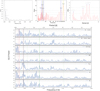 |
Fig. 3 Periodograms. Top row, left panel: window function of HARPS-N RVs, with its highest peaks highlighted. Top row, middle panel: GLS periodogram of HARPS-N RVs. Two yellow vertical lines are drawn at the periodicity of BD+00 444b transits (15.67 days) and the highest peak of the GLS, while their aliases due to the window function (respectively ≈219 and 420 days), are identified by blue vertical lines. Top row, right panel: MLP of HARPS-N RVs between 10 and 20 days, with its major peak identified at precisely 15.67 days. The three horizontal lines represent the FAP levels of 10%, 1%, and 0.1%. Bottom panel: GLS periodogram of the HARPS-N RV residuals of the one-planet and two-planet models (first two rows), and of various activity indices specified in the labels. The main peak of the RV GLS periodogram, which is here identified as the signal of planet candidate BD+00 444c at about 97 d, is highlighted with a red vertical line, while the period of the transiting candidate (15.67 d) and the possible stellar rotation period (45 d) are highlighted in green and gray, respectively. Shaded vertical bars are plotted at 0.5× and 2× the respective signals to emphasize potential aliases. The horizontal dashed lines mark, respectively, the 10% and 1% confidence levels (evaluated with the bootstrap method). |
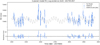 |
Fig. 4 HARPS-N RV measurements of BD+00 444 in blue and the preferred model fit in black, along with the RV residuals over the model fit. The small error bars represent the formal RV uncertainties, while the larger error bars account for uncertainties increased by the best-fit jitter term (σw). |
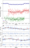 |
Fig. 5 Phase-folded plots. Top panel: global fit result for TESS and the ground-based transits. Both LCOGT light curves are shifted on the y-axis for clarity, and their respective filter band are indicated in the legend, while the superimposed points represent ~30-minute bins. Bottom panels: phase-folded HARPS-N RVs to the period of planet b and candidate c, along with their residuals. The red circles represent the average value of ~10 phased RV data points at a time. |
4.3 HARPS-N detection sensitivity
We estimated the completeness of the HARPS-N RV time series by performing injection-recovery simulations, in which synthetic RVs with planetary signals were injected at the times of our observations, using HARPS-N error bars and the estimated stellar jitter included in Sect. 6. We simulated the signals of additional companions across a logarithmic 30 × 30 grid in planetary mass (Mp) and semi-major axis (a), covering the ranges 0.01–20 MJup (or Jupiter masses) and 0.01–10 au. As in Bonomo et al. (2023), for each location of the grid we generated 100 synthetic planetary signals, drawing a and Mp from a log-uniform distribution inside the cell, T0 from a uniform distribution in [0, P], the orbital inclination i from a uniform cos i distribution in [0, 1], ω from a uniform distribution in [0, 2π], and e from a beta distribution in [0.0, 0.8] (Kipping 2013). We fitted the signals by employing either Keplerian orbits or linear and quadratic trends, in order to take into account long-period signals, which would not be correctly identified as Keplerian due to the short time span of the RV observations (550 d). We then adopted the Bayesian information criterion (BIC) to compare the fitted planetary model with a constant model and considered the planetary signal significantly detected only when ∆BIC > 10 in favor of the planet-induced one. The detection fraction was finally computed as the portion of detected signals for each grid element, as illustrated by Fig. 6.
5 Discussion
5.1 The non-transiting candidate BD+00 444 c
We infer that the true mass of BD+00 444 c should lie within a factor of 2 of the minimum mass ( ). This is because the probability that its orbital inclination lies between 30 deg and 90 deg is ~87% (Fischer et al. 2014), without even taking into account the existence of the close-in transiting planet, with an inclination of ~90 deg. The predicted time of transit of BD+00 444 c is outside the region observed by TESS, and its host star will not be observed in the upcoming TESS sectors (at least up to early 2026). However, with an estimated posterior transit probability of ~1%, adopting the formulation given by Stevens & Gaudi (2013) and assuming e = 0, it is possible that the candidate is not transiting at all. Therefore, we expect that the planet will necessitate more RV measurements to be secured with higher statistical evidence.
Interestingly, BD+00 444 c has an equilibrium temperature of 283 ± 4 K (assuming zero Bond albedo and uniform heat redistribution to the night side) that would place it within the habitable zone (Fig. 7). Despite its location, this planet likely has a Neptune-type composition, which would render it inhospitable for life as we know it. Nevertheless, a moon orbiting this planet might harbor conditions suitable for the development of life (see, e.g., Martínez-Rodríguez et al. 2019).
Planet parameters.
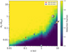 |
Fig. 6 HARPS-N RV detection map for BD+00 444. The color scale expresses the detection fraction (i.e., the detection probability), while the circles mark the position of BD+00 444 b (in red) and candidate BD+00 444 c (in blue), for which we use Mp sin i. Jupiter, Saturn and the Earth are shown for comparison. |
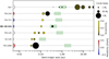 |
Fig. 7 System architectures featuring inner transiting planets with masses below 20 M⊕ (represented with different circle sizes) and eccentricities of greater than 0.10 (represented with yellow color), determined with at least 5σ confidence. The shaded green rectangles represent the respective habitable zones, while the host metallicity and size are illustrated by color and circle size, respectively. The Solar System is included for comparison. |
5.2 Composition of BD+00 444 b
We employed an advanced interior model to study BD+00 444 b, where water can be present in the core, the mantle, and surface depending on the specific thermal state of the planet. The model is based on that of Dorn et al. (2017) with recent adaptations as presented by Luo et al. (2024). For this application, we focused on interiors with Earth-like rocky interiors with H2-He atmospheres, water steam atmospheres, and atmospheres containing a mixture of water and H2-He. In the last case, we considered two different envelope structures: a homogeneously mixed atmosphere consisting of H2-He and water, and a differentiated structure where the water and H2-He layers are separated, with the pure water layer below the pure H2-He layer. Although the homogeneous envelope is more realistic, we added the layered case for comparison.
We considered a core made of Fe with the light alloy elements H and O. For solid Fe, we used the equation of state for hexagonal close packed iron (Hakim et al. 2018; Miozzi et al. 2020). For liquid iron and iron alloys, we use the equation of state by Luo et al. (2024). The core thermal profile is assumed to be adiabatic. At the core-mantle boundary, there is a temperature jump as the core can be hotter than the mantle due to the residual heat released during core formation following Stixrude (2014).
The mantle is assumed to be made up of three major constituents, i.e., MgO, SiO2, and FeO. For the solid mantle, we used the thermodynamical model Perple_X (Connolly 2009) to compute stable mineralogy and density for a given composition, pressure, and temperature, employing the database of Stixrude & Lithgow-Bertelloni (2022). For pressures higher than ~ 125 GPa, we defined stable minerals a priori and used their respective equation of states from various sources (Hemley et al. 1992; Fischer et al. 2011; Faik et al. 2018; Musella et al. 2019). For the liquid mantle, we calculated its density assuming an ideal mixture of the main components (Mg2SiO4, SiO2, and FeO) (Melosh 2007; Faik et al. 2018; Ichikawa & Tsuchiya 2020; Stewart et al. 2020) and added them using the additive volume law. We used Mg2SiO4 instead of MgO since the data for forsterite was recently updated for the high-pressure temperature regime (Stewart et al. 2020), which is not available for MgO to our knowledge. The mantle is assumed to be fully adiabatic.
Water can be present in mantle melts, while solid mantle is assumed to be dry. The addition of water reduces the density, for which we follow Bajgain et al. (2015). For small water mass fractions, this reduction is nearly independent of pressure and temperature. The melting curve of mantle material is calculated for dry and pure MgSiO3. The addition of water (Katz et al. 2003) and iron (Dorn et al. 2018) can lower the melting temperatures. Water added to the core also lowers its melting temperature, for which we followed Luo et al. (2024). Possible water in the core may be present in both liquid and solid phases. The partitioning between mantle melts and the water layer is determined by Henry’s law, for which we used the fitted solubility function of Dorn & Lichtenberg (2021). For the partitioning of water between iron and silicates, we followed Luo et al. (2024). For the equilibration pressure of water to partition between iron and silicates, we used half of the core-mantle boundary pressure, which is within typically discussed values for Earth (0.3–0.6). Varying this pressure would introduce overall small changes in the distribution of water.
On BD+00444 b water can be in steam or supercritical phase, for which we use the AQUA (Haldemann et al. 2020) compilation of equation of states. For pressures below 0.1 bar, we assumed an isothermal profile and then switched to an adiabatic profile. Whenever we considered H2-He, we followed the model of Guillot (2010) for an irradiated atmosphere and an underlying gaseous envelope. If H2O and H2-He are fully mixed, we adjust the metallicity Z of the envelope according to
 (1)
(1)
where  and
and  are the total H2O and H2-He mass of the envelope respectively. Further details on the structure models can be found in Dorn et al. (2017).
It is possible to match the bulk properties of BD+00444 b with all four structure models. In the left panel of Fig. 8, we show mass-radius relations between known transiting exoplanets6 and classical layered structure models by Zeng & Sasselov (2013), while, in the right panel, we display the resulting relations from our best-fit parameters. For a pure water-world planet without any H2-He, the bulk properties of BD+00 444 b are consistent with a water mass fraction of 60–65%. This is slightly higher than the commonly used upper limit of 50% (Luque & Pallé 2022). However, the atmosphere contains only 6.2–7.5% of the total water content. The majority of the water is stored in the interior of the planet. Considering the other extreme case, where no water is present on the planet, the bulk properties are consistent with a H2-He mass fraction of 4.5 ± 0.5%. More realistically, the atmosphere of the planet contains both water and H2-He. If the two components are separate, the water mass fraction is 40% with 2.0 ± 0.4% H2-He. If, on the other hand, the H2O and H2-He are fully mixed, the bulk properties are consistent with a water fraction of 50% and a H2-He fraction of 2.2 ± 0.5%.
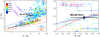 |
Fig. 8 Mass-radius diagram. Left panel: planetary masses and radii of the known transiting exoplanets. The colors of the planets correspond to their equilibrium temperatures. The iso-composition curves for differentiated planets (Zeng & Sasselov 2013) are described in the legend. Right panel: zoom-in of the same diagram in mass linear scale, displaying the different compositions that best match the mass and radius of BD+00 444 b with both differentiated and miscible interiors (Sect. 5.2). |
5.3 Formation and evolution
We investigated the possible formation history of BD+00 444’s two planets following the approaches described by Mantovan et al. (2024) and Damasso et al. (2024). We used our Monte Carlo version of the GroMiT (planetary GROwth and MIgration Tracks) code (Polychroni et al. 2023) to simulate the possible formation tracks of planets b and c in the framework of the pebble accretion scenario. In particular, we employed the treatments for the growth and migration of pebble-accreting and gas-accreting planets from Johansen et al. (2019) and Tanaka et al. (2020) and the scaling law for the pebble isolation mass from Bitsch et al. (2018).
The planet formation model builds on the description of the viscously evolving circumstellar disk in which the planets are embedded (Johansen et al. 2019; Armitage 2020) complemented by the prescriptions for the characterization of its thermal profile due to the interplay between viscous heating and stellar irradiation from Ida et al. (2016), and of its solid-to-gas ratio profile from Turrini et al. (2023). The stellar luminosity during the pre-main sequence phase was set to 0.85 L⊙ based on the stellar evolutionary models from Baraffe et al. (2015) for stars with the mass of BD+00 444 at the age of 1 Myr.
We ran two sets of simulations considering a millimeter-sized (mm-sized) pebble-dominated disk and a centimeter-sized (cm-sized) one, each one simulating the formation of 2×10⁵ individual planets by randomly varying the formation time and the initial semi-major axis of their planetary seeds, as well as the disk viscosity coefficient, a. We kept the rest of the physical characteristics of the disk constant for all runs; see Table 3 for more details. In Fig. 9 we plot the complete results of our simulations, as well as the locations where planet b and candidate c fall in.
We considered as successful those solutions where the resulting objects have (i) final mass within 1σ of the reported mass of each one (in the case of candidate c we focus on its minimum mass) and (ii) final semi-major axis within half and twice the nominal semi-major axis of each planet, to account for the uncertainty of the planetary migration rates (e.g., Pirani et al. 2019). These solutions are plotted in Fig. 10. We found that the modeled system can create a few massive planets, in line with its reported low metallicity. All successful synthetic planets emerge from planetary seeds that formed within the first 1 Myr of the disk’s lifetime, with the planet b’s solutions starting their growth on average slightly later than the planet c’s.
In the cm-sized pebble-dominated disk, the successful solutions of both planets start forming beyond 7 au (on average at 8 au for planet b and at 11 au for planet c) and need their planetary seed to appear very early in the disk’s lifetime (within the first 0.4 Myr) to successfully gather the required mass and migrate inwards. In the mm-sized pebble-dominated disk, both planets start their formation within 4 au (on average 3.0 au and 3.6 au respectively) and their seeds appear later, up to 0.7 Myr. Also in this case candidate planet c generally starts its growth a bit earlier than planet b.
Regardless of the specific planet and pebble size, all successful solutions complete the growth of their core at about the same time within a similar turbulent environment (α = 0.0022–0.0028), forming similar cores of 2.0–2.5 M⊕. While we cannot differentiate between the cases of mm-sized and cm-sized pebbles based solely on the physical characteristics of the two planets, there are some conclusions that we can reach. Candidate planet c needs to start its formation earlier and further out than planet b, in order to reach its reported minimum mass in all scenarios. However, given that the two planetary cores complete their growth pretty much by the same time (i.e., the growth of planet c is slower than that of planet b) it is unlikely that the outer object experienced close encounters with the inner one during the formation stages.
To gain further insight into the possible formation environment of BD+00 444’s planetary system, we compared the core masses emerging from our planet formation model for planet b with those allowed by the mass-radius relationships for the cores and the gaseous envelopes from Fortney et al. (2007) and Lopez & Fortney (2014). Based on the results on the planetary compositions compatible with BD+00 444 b’s characteristics discussed in Sect. 5.2 and the formation separations discussed above, we explored three core compositions. The first one is an ice-rich core composition described by Eq. (7) from Fortney et al. (2007) where we set the water ice mass fraction in the core to 0.33 based on the mass balance between rocks and ices from Turrini et al. (2021). The second one is a rocky composition based on Eq. (8) from Fortney et al. (2007) where the rock mass fraction in the core is set to 0.66 to assume an Earth-like composition. The last one is the simplified treatment for a rock-iron core from Eq. (2) of Lopez & Fortney (2014).
For the envelope, we considered both the cases of solar metallicity and enhanced (50× solar) metallicity from Lopez & Fortney (2014). Given the mature age of BD+00 444’s star, however, the differences in the envelope radii associated with these two compositions are significantly smaller than those due to the other parameters that we sampled. As in Damasso et al. (2024), for each combination of core-envelope compositions, we performed 106 Monte Carlo extractions where we randomly sampled the core mass fraction, stellar age, and planetary mass. The core mass fraction is extracted from a uniform distribution between 0 and 1, while the stellar age and planetary mass are extracted from normal distributions truncated to zero whose widths are set by the uncertainties on the two parameters.
The results of our Monte Carlo exploration are shown in Fig. 11 for the case of enhanced envelope metallicity, which is likely more realistic for sub-Neptunian planets based on the case of the ice giants in the Solar System (e.g., de Pater et al. 2023, and references therein) and the mass-metallicity relationships of giant planets from Thorngren et al. (2016). The solutions shown are those that fall within 3σ from the estimated planetary mass, radius, and density from Table 2. The results for the solar metallicity envelope are qualitatively identical. While the interior models adopted are less detailed than those discussed in Sect. 5.2, Fig. 11 immediately shows that the characteristics of BD+00 444 b do not allow for core masses as small as those set by the pebble isolation mass shown in Fig. 10.
As discussed by Mantovan et al. (2024) and Damasso et al. (2024), however, the core masses set by the pebble isolation mass are actually lower limits because the population synthesis simulations do not account for two processes that can increase the final core mass. The first one is the accretion of planetesimals if the native protoplanetary disk was characterized by comparable abundances of pebbles and planetesimals, as it would allow the core to grow beyond the pebble isolation mass. The second one is the accretion of high-metallicity gas enriched by the volatiles released by the ices sublimating from the inward drifting pebbles if the protoplanetary disk was pebble-dominated. The high-metallicity gas could mimic the effects of a more massive core like those suggested by the interior studies of Jupiter (Wahl et al. 2017; Stevenson 2020) and Saturn (Mankovich & Fuller 2021).
The marked eccentricity of planet b allows for a third possibility. While the candidate nature of planet c and the lack of more detailed constraints on its orbit and mass hinder the quantification of the dynamical excitation of the systems (Chambers 2001; Turrini et al. 2020), the orbital eccentricity of planet b is highly suggestive of chaotic phases of dynamical evolution in its past (Weidenschilling & Marzari 1996; Chambers 2001; Zinzi & Turrini 2017). Unless its mass proves significantly higher than its currently estimated lower bound, the possible circular orbit for planet c may indicate that it was not the planetary body that chaotically interacted with planet b.
Since collisions are the most likely outcome of chaotic evolution (Chambers 2001; Zinzi & Turrini 2017; Turrini et al. 2020), the currently observed planet b could be the result of the giant impact between two separate planetary bodies that reached the pebble isolation mass in a higher-multiplicity primordial planetary system. The higher core mass than what would be suggested by the pebble isolation mass profile alone could then be the result of the merging of the cores of these two planets. Collisions lead to the damping of the orbital eccentricity of the surviving body (Chambers 2001), implying that the pre-collision eccentricity of planet b was higher than its current value. This, in turn, would have increased the likelihood of planetary collisions given the compact architecture of the system.
While these alternative scenarios for the formation environments and physical characteristics of BD+00 444’s planets cannot be discriminated based on the current data, future observations aimed at compositionally characterizing the atmosphere of planet b have the potential to provide critical insight into the past of this system. If the two planets formed in a pebble-dominated disk, their atmospheres are expected to be highly enriched in the volatile elements C and O (and possibly N) and limited or not enriched at all in more refractory ones (Booth & Ilee 2019; Turrini et al. 2021; Schneider & Bitsch 2021).
If the two planets formed in planetesimal-rich disks or if planet b is the result of a giant impact between two previously existing planets, the atmospheric composition of planet b should show higher enrichment in S and refractories than in C and O (Turrini et al. 2021; Pacetti et al. 2022). Observational constraints on the S-over-N (Turrini et al. 2021; Pacetti et al. 2022) or C-over-S (Crossfield 2023) abundance ratios could allow to shed light on the characteristics of BD+00 444’s formation history. Similarly, the scenarios dominated by mm-sized and cm-sized pebbles could be discriminated by constraining the enrichment of planet b in the volatile elements C, O, and N. Planets forming in disks dominated by cm-sized pebbles are expected to be characterized by enrichment in volatile elements of an order of magnitude or higher with respect to the host star, while mm-sized pebbles are expected to produce less marked enrichment (Booth & Ilee 2019; Schneider & Bitsch 2021).
Input parameters used to run the MC modified GroMiT code to produce simulated planets and investigate the formation history of TOI-2443 b.
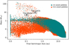 |
Fig. 9 Synthetic populations of planets resulting from the two Monte Carlo runs of 2×10⁵ extractions each with GroMiT. The plot shows the final masses and orbital periods of the simulated growth tracks. The vermilion symbols indicate those planets formed in disks dominated by mm-sized pebbles, while with cactus green we denote cm-sized pebble-dominated disks. Planets b and c are indicated using two larger cyan circles and the boxes around them highlight the region of parameter space populated by the successful solutions. |
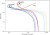 |
Fig. 10 Planetary growth tracks that satisfy the selection conditions associated with the black boxes in Fig. 9. The growth tracks are projected in the semi-major axis-planetary mass space. The blue tracks denote the successful solutions for planet b while the red ones are those of planet c. The solid lines indicate the planets that formed in an mm-sized pebble-dominated disk, while the dotted ones formed in a cm-sized one. Miso denotes the pebble isolation mass above which no pebbles are able to accrete onto the forming planet (Lambrechts & Johansen 2014). |
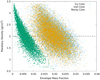 |
Fig. 11 Monte Carlo investigation of the spread in the planetary density and the envelope mass fraction of planet b resulting from the uncertainties on the stellar age, the planetary mass and radius, and the composition of the core under the assumption of enhanced metallicity of the planetary envelope. The three combinations of symbols and colors identify the three compositions and mass-radius relationships explored for the core, while the horizontal dashed line marks the retrieved bulk density of planet b (without uncertainties for better clarity). |
5.4 Tidal timescales and dissipation inside BD+00444 b
The large spatial ratio a/R* and small mass ratio Mp /M* of planet b make its tidal influence on the star negligible. In other words, it does not affect the orbit semi-major axis, stellar rotation, or the orientation of the stellar spin in any significant way. On the other hand, the tides raised by the star on planet b are relevant for its rotation and internal dissipation of tidal energy. We adopted the constant time-lag model by Leconte et al. (2010) where we express the product of the Love number k2p of the planet by its tidal time lag ∆tp using the formula k2p∆tp = (2/3)Q′p/n, where Q′p is the modified tidal quality factor of the planet and n = 2π/Porb is its orbital mean motion with Porb being its orbital period. The advantage of a constant time-lag model is its validity for large values of eccentricity as in the case of BD+00444 b.
The modified tidal quality factors of mini-Neptune planets are largely unknown. Using Uranus or Neptune as analogs for their tidal dissipation, one can adopt Q′p values between 4 × 10⁴ and 1.5 × 10⁵ and consider k2p = 0.3–0.4 (Tittemore & Wisdom 1990; Zhang & Hamilton 2008; Ogilvie 2014; James & Stixrude 2024). Assuming for simplicity a value of Q′p= 105, we obtained an e-folding decay timescale of the orbital eccentricity  Gyr for BD+00444 b, much longer than Hubble time. This implies that tidal effects likely do not affect the eccentricities of planets b and c. The power dissipated by the tides inside planet b is Ptide ~ 8 × 10¹⁴ W for the present value of its eccentricity of eb ≈ 0.3. Both Ptide and
  scale proportionally to (Q′p)−1, so our estimate of Ptide is rather conservative. It is comparable to or even larger than the average extreme ultraviolet (XUV7) flux received by the planet from its host star, which we estimated to be LXUV ~ 3.2 × 10¹⁴ W in the pass-band from 0.1 to 92 nm where photons can induce ionization and photo-evaporation of a hydrogen-rich planetary atmosphere. This estimate of LXUV is based on the tables by Johnstone et al. (2021) considering a rotation period of the star of ~45 days, and is uncertain by at least a factor of a few due to the variable activity level at a given rotation period and the large uncertainty on the stellar rotation period (cf. Sect. 4.1).
Another consequence of the eccentric orbit of planet b is the pseudo-synchronization of its rotation, which is faster than the orbital period. For the present value of its eccentricity, the pseudo-synchronous rotation period is 10.1 days and the timescale for attaining pseudo-synchronization is of ~2.5 Myr for Q′p = 105 (see below for the indirect effect of the other planet).
The analysis presented above assumes the present value of the eccentricity of planet b. In fact, the perturbations due to planet c produce a secular exchange of angular momentum between the orbits, while their energies and their semi-major axes are secularly constant because this is a non-resonant system. The angular momentum exchanges induce a modulation of the eccentricities values. Unfortunately, the inclination of the planet’s c orbit is unknown and its eccentricity only has an upper limit (Table 2). Therefore, a precise prediction of the amplitude and the period of the eccentricity modulations is not possible. A simplified treatment that can provide order-of-magnitude estimates is based on the model by Mardling (2007) that assumes co-planarity of the orbits of the two planets and a small eccentricity of the inner planet to allow the development of the secular perturbation equations to the first order in its eccentricity.
Adopting Mardling’s simplifying hypotheses and considering that tides cannot significantly affect the eccentricities of the planetary orbits in our system, the angle η = ϖb − ϖc between the arguments of periapsis of the two planets can be librating or circulating (see Sect. 3 of Mardling 2007, for details). The period of libration or circulation of η is equal to the period of the modulation of the orbital eccentricity of planet b, and is given in the top panel of Fig. 12 as a function of the unknown value of the eccentricity of the outer planet c. In any case, it turns out to be shorter than ~6 × 10⁴ yr, that is, much shorter than the pseudo-synchronization timescale of planet rotation. Therefore, we expect that the rotation of the planet synchronizes with the value corresponding to its average eccentricity.
The short modulation period of the eccentricity eb of planet b implies that its present value may not be representative of the actual mean tidal dissipation inside the planet. In other words, being interested in the average value of the tidal power Pdiss dissipated inside planet b on evolutionary timescales, the fundamental parameter that we need is the mean value of its squared eccentricity  . The minimum value of
  is obtained when the angle η circulates and is equal to
 ![Mathematical equation: ${\left[ {e_{\rm{p}}^{({\rm{eq}})}} \right]^2}/2$](/articles/aa/full_html/2025/01/aa51859-24/aa51859-24-eq70.png) , where
, where  is the equilibrium eccentricity of planet b as given by Eq. (36) of Mardling (2007) and is a function of, among others, the unknown eccentricity of planet c (see lower panel of Fig. 12, black line). The average dissipated power inside planet b as a function of its equilibrium eccentricity is plotted in the lower panel of Fig. 12 (red line) and is computed by means of Eqs. (1) and (2) of Mardling (2007) adopting Qp/k2p = 2Q′p/3 and Q′p = 105. Mardling’s second-order formula in the eccentricity provides systematically lower values of Pdiss than the higher-order model by Leconte et al. (2010), which is in line with our estimate of a lower value for the tidal power and the poorly known value of Q′p for our planet.
Looking at the lower panel of Fig. 12, we conclude that the power dissipated by the tides inside planet b becomes comparable with the XUV flux received from the star when its equilibrium eccentricity is of ~0.3 or larger. In turn, such an eccentricity of the inner planet b implies a rather large eccentricity of the outer planet c that, in our simplified model, must be larger than ~0.5, which is close to or above the lower limit as derived by the 2-planet model (see Sect. 4.2 and Table 2).
Finally, we considered the case of a strong tidal dissipation inside planet b, appropriate for a planet with a mainly solid interior, a possibility that cannot be excluded given the kind of structure models considered in Sect. 5.2. Adopting Q′p = 300 (Henning et al. 2009), the eccentricity e-folding decay time τe ~ 1.9 Gyr, while the tidal power dissipated inside the planet becomes of 2.6 × 10¹⁷ W for eb = 0.3 corresponding to a surface heat flux of ~90 W m−2, that is, about 30 times larger than in the case of the Jupiter moon Io, suggesting a very strong volcanic activity potentially detectable by means of dedicated spectroscopic transit observations. In the presence of the outer planet c, the strong tidal dissipation inside planet b would drive its eccentricity toward its equilibrium value  over a timescale of a few τe ’s, comparable with the age of the system, given that BD+00 444 is likely to be an old star (see Sect. 3.3 of Mardling 2007). In this scenario, the current value of the eccentricity would be close to the equilibrium value implying a rather large eccentricity of planet c (ec ~ 0.5, cf. Fig. 12, lower panel) and an extended phase of remarkable tidal dissipation inside planet b with an average Pdiss of the order of 1017 W. Such predictions of a huge internal tidal heating in planet b and of a rather large eccentricity of planet c can provide observational tests for such a high tidal dissipation regime resulting from a low Q′p value.
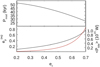 |
Fig. 12 Circulation and eccentricity plot. Top panel: circulation or libration period Pmod of the angle ŋ vs. the eccentricity ec of the outer planet c in the BD+00 444 system. The modulation of the eccentricity eb of the orbit of the inner planet occurs with the same period. Lower panel: the equilibrium eccentricity |

5.5 Atmospheric prospects for BD+00 444 b
The exceptionally high TSM of BD+00 444 b of  (Table 2) makes it an ideal candidate for atmospheric characterization with JWST. This metric indicates that its atmosphere is well-suited for in-depth study via transmission spectroscopy, offering an opportunity to detect key molecular features. Interestingly, only three other sub-Neptunes with 2 R⊕ < Rp < 3 R⊕, orbiting around FGK stars, have higher TSM values (i.e., HD 136352 c, HD 191939 d, and TOI-544b, respectively from Delrez et al. 2021; Orell-Miquel et al. 2023; Osborne et al. 2024), as depicted in Fig. 13, to the best of our knowledge.
The highly dissipative tidal scenario (cf. Sect. 5.3) suggests strong volcanic activity on planet b, which could potentially be detected through spectroscopic observations during transits. In this scenario, the eccentricity of BD+00 444 b would be maintained by perturbations by candidate planet c, whose orbit would also be highly eccentric (ec ~ 0.5). Alternatively, the rather large orbital eccentricity of planet b might have also originated from a primordial impact and persisted due to rheological properties similar to that of Uranus or Neptune, resulting in minimal eccentricity damping over time (cf. Sect. 5.4). Furthermore, investigating the atmosphere of BD+00 444 b would allow us to constrain its water content, which in our models can span between null and 66%, and learn whether the planet is rich in volatile elements (likely a consequence of a cm-sized pebble-dominated formation disk), while comparing S, C, and 0 enrichment may provide a clue on whether BD+00 444 b formed in a planetesimal-rich disk and possibly underwent a giant impact.
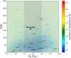 |
Fig. 13 TSM values over the radius of planets with well-characterized radius and mass (with 5σ, 4σ accuracy, respectively) orbiting around FGK stars. The color of the points represents their equilibrium temperature, while the TSM error bars are suppressed for clarity. |
6 Summary
Thanks to precise RV measurements obtained with the high-resolution spectrograph HARPS-N, we determined the mass of BD+00 444 b to be 4.8 ± 1.1 M⊕. With a radius of 2.36 ± 0.05 R⊕, this transiting sub-Neptune, initially discovered by TESS, is on an eccentric orbit ( ) of about 15.67 days around a quiet K5 V star (Table 1), and has a bulk density of
  g cm−3. In particular, BD+00 444 b is found to have a high TSM of
  and is therefore an optimal candidate for atmospheric follow-up with JWST.
While we can exclude the presence of Neptune-mass planets up to 1 au, and Jupiter-mass planets up to 10 au (Fig. 6), unless severely inclined with respect to the orbital plane of BD+00 444 b, our analysis suggests the existence of another planet. Candidate BD+00 444 c, on a longer orbital period of about 97 days (~0.4 au), has an equilibrium temperature of 283 ± 4 K, which would place it within the habitable zone, and a minimum mass, Mc sin i, of  , which likely lies within a factor of 2 of the true mass (i.e., it is barely more massive than Neptune). However, we expect this candidate to be non-transiting, and therefore its confirmation will require further RV measurements and more robust statistical evidence.
Data availability
The RV data collected for this article have been uploaded to Zenodo along with additional plots and tables.
Acknowledgements
We would like to thank the referee J.A. Caballero for giving many constructive comments that substantially helped improving the quality of the paper. We acknowledge financial contribution from the INAF Large Grant 2023 “EX0DEM0”. This work is based on observations made with the Italian Telescopio Nazionale Galileo (TNG) operated by the Fundación Galileo Galilei (FGG) of the Istituto Nazionale di Astrofisica (INAF) at the Observatorio del Roque de los Muchachos (La Palma, Canary Islands, Spain). We acknowledge the Italian center for Astronomical Archives (IA2, https://www.ia2.inaf.it), part of the Italian National Institute for Astrophysics (INAF), for providing technical assistance, services and supporting activities of the GAPS collaboration. This work includes data collected with the TESS mission, obtained from the MAST data archive at the Space Telescope Science Institute (STScI). Funding for the TESS mission is provided by the NASA Explorer Program. STScI is operated by the Association of Universities for Research in Astronomy, Inc., under NASA contract NAS 5–26555. We acknowledge the use of public TESS data from pipelines at the TESS Science Office and at the TESS Science Processing Operations Center. Resources supporting this work were provided by the NASA High-End Computing (HEC) Program through the NASA Advanced Supercomputing (NAS) Division at Ames Research Center for the production of the SPOC data products. Funding for the TESS mission is provided by NASA’s Science Mission Directorate. K.A.C. and C.N.W. acknowledge support from the TESS mission via sub-award s3449 from MIT. This work makes use of observations from the LCOGT network. Part of the LCOGT telescope time was granted by NOIRLab through the Mid-Scale Innovations Program (MSIP). MSIP is funded by NSF. This research made use of the Exoplanet Follow-up Observation Program (ExoFOP; DOI: 10.26134/ExoFOP5) website, which is operated by the California Institute of Technology, under contract with the National Aeronautics and Space Administration under the Exoplanet Exploration Program. The research made use of the SIMBAD database, operated at CDS, Strasbourg, France, NASA’s Astrophysics Data System and the NASA Exoplanet Archive, which is operated by the California Institute of Technology, under contract with the National Aeronautics and Space Administration under the Exoplanet Exploration Program. The work is based on observations made with the Italian Telescopio Nazionale Galileo (TNG) operated on the island of La Palma by the Fundacion Galileo Galilei of the INAF (Istituto Nazionale di Astrofisica) at the Spanish Observatorio del Roque de los Muchachos of the Instituto de Astrofisica de Canarias. This publication makes use of The Data & Analysis Center for Exoplanets (DACE), which is a facility based at the University of Geneva (CH) dedicated to extrasolar planets data visualization, exchange and analysis. DACE is a platform of the Swiss National Centre of Competence in Research (NCCR) PlanetS, federating the Swiss expertise in Exoplanet research. The DACE platform is available at https://dace.unige.ch. This work also made use of data from the European Space Agency (ESA) mission Gaia (https://www.cosmos.esa.int/gaia), processed by the Gaia Data Processing and Analysis Consortium (DPAC, https://www.cosmos.esa.int/web/gaia/dpac/consortium). L.M. acknowledges financial contribution from PRIN MUR 2022 project 2022J4H55R. D.P. acknowledges the support from the Istituto Nazionale di Oceanografia e Geofisica Sperimentale (OGS) and CINECA through the program “HPC-TRES (High Performance Computing Training and Research for Earth Sciences)” award number 2022-05 as well as the support of the PRIN INAF 2019 “Planetary systems at young ages (PLATEA)”. D.T. and D.P. acknowledge the support from the ASI-INAF grant no. 2021-5-HH.0 plus addenda no. 2021-5-HH.1-2022 and 2021-5-HH.2-2024 as well as the computational support of the Genesis cluster at INAF-IAPS. D.T. acknowledges the support of the European Research Council via the Horizon 2020 Framework Programme ERC Synergy “ECOGAL” Project GA-855130. M.P. acknowledges support from the European Union – NextGenerationEU (PRIN MUR 2022 20229R43BH) and the “Programma di Ricerca Fondamentale INAF 2023”. C.D. and M.S. acknowledge support from the Swiss National Science Foundation under grant TMSGI2_211313. X.D. acknowledges the support from the European Research Council (ERC) under the European Union s Horizon 2020 research and innovation programme (grant agreement SCORE No. 851555) and from the Swiss National Science Foundation under the grant SPECTRE (No 200021_215200).
References
- Allard, F., Homeier, D., & Freytag, B. 2012, Philos. Trans. Roy. Soc. Lond. Ser. A, 370, 2765 [NASA ADS] [Google Scholar]
- Aller, A., Lillo-Box, J., Jones, D., Miranda, L. F., & Barceló Forteza, S. 2020, A&A, 635, A128 [NASA ADS] [CrossRef] [EDP Sciences] [Google Scholar]
- Almeida-Fernandes, F., & Rocha-Pinto, H. J. 2018, MNRAS, 476, 184 [Google Scholar]
- Alqasim, A., Grieves, N., Rosário, N. M., et al. 2024, MNRAS, 533, 1 [Google Scholar]
- Amard, L., Roquette, J., & Matt, S. P. 2020, MNRAS, 499, 3481 [NASA ADS] [CrossRef] [Google Scholar]
- Armitage, P. J. 2020, Astrophysics of Planet Formation, 2nd edn. (Cambridge University Press) [CrossRef] [Google Scholar]
- Astropy Collaboration (Price-Whelan, A. M., et al.) 2018, AJ, 156, 123 [Google Scholar]
- Badenas-Agusti, M., Günther, M. N., Daylan, T., et al. 2020, AJ, 160, 113 [NASA ADS] [CrossRef] [Google Scholar]
- Bajgain, S., Ghosh, D. B., & Karki, B. B. 2015, Nat. Commun., 6, 8578 [NASA ADS] [CrossRef] [Google Scholar]
- Baraffe, I., Homeier, D., Allard, F., & Chabrier, G. 2015, A&A, 577, A42 [NASA ADS] [CrossRef] [EDP Sciences] [Google Scholar]
- Baranne, A., Queloz, D., Mayor, M., et al. 1996, A&AS, 119, 373 [NASA ADS] [CrossRef] [EDP Sciences] [Google Scholar]
- Barnes, S. A., Weingrill, J., Fritzewski, D., Strassmeier, K. G., & Platais, I. 2016, ApJ, 823, 16 [Google Scholar]
- Bean, J. L., Raymond, S. N., & Owen, J. E. 2021, J. Geophys. Res. (Planets), 126, e06639 [NASA ADS] [Google Scholar]
- Biazzo, K., Bozza, V., Mancini, L., & Sozzetti, A. 2022a, in Demographics of Exoplanetary Systems, Lecture Notes of the 3rd Advanced School on Exo-planetary Science, eds. K. Biazzo, V. Bozza, L. Mancini, & A. Sozzetti, Astrophysics and Space Science Library, 466, 143 [NASA ADS] [CrossRef] [Google Scholar]
- Biazzo, K., D’Orazi, V., Desidera, S., et al. 2022b, A&A, 664, A161 [NASA ADS] [CrossRef] [EDP Sciences] [Google Scholar]
- Bitsch, B., Morbidelli, A., Johansen, A., et al. 2018, A&A, 612, A30 [NASA ADS] [CrossRef] [EDP Sciences] [Google Scholar]
- Bonomo, A. S., Dumusque, X., Massa, A., et al. 2023, A&A, 677, A33 [NASA ADS] [CrossRef] [EDP Sciences] [Google Scholar]
- Booth, R. A., & Ilee, J. D. 2019, MNRAS, 487, 3998 [CrossRef] [Google Scholar]
- Borucki, W. J., Koch, D., Basri, G., et al. 2010, Science, 327, 977 [Google Scholar]
- Brandt, T. D. 2021, ApJS, 254, 42 [NASA ADS] [CrossRef] [Google Scholar]
- Brewer, J. M., Fischer, D. A., Valenti, J. A., & Piskunov, N. 2016, ApJS, 225, 32 [Google Scholar]
- Brown, T. M., Baliber, N., Bianco, F. B., et al. 2013, PASP, 125, 1031 [Google Scholar]
- Bryson, S. T., Jenkins, J. M., Klaus, T. C., et al. 2010, SPIE Conf. Ser., 7740, 77401D [NASA ADS] [Google Scholar]
- Bryson, S. T., Jenkins, J. M., Klaus, T. C., et al. 2020, Kepler Data Processing Handbook: Target and Aperture Definitions: Selecting Pixels for Kepler Downlink, Kepler Science Document KSCI-19081-003 [Google Scholar]
- Burt, J. A., Dragomir, D., Mollière, P., et al. 2021, AJ, 162, 87 [NASA ADS] [CrossRef] [Google Scholar]
- Capitanio, L., Lallement, R., Vergely, J. L., Elyajouri, M., & Monreal-Ibero, A. 2017, A&A, 606, A65 [NASA ADS] [CrossRef] [EDP Sciences] [Google Scholar]
- Casagrande, L., Lin, J., Rains, A. D., et al. 2021, MNRAS, 507, 2684 [NASA ADS] [CrossRef] [Google Scholar]
- Castelli, F., & Kurucz, R. L. 2003, in Modelling of Stellar Atmospheres, 210, eds. N. Piskunov, W. W. Weiss, & D. F. Gray, A20 [NASA ADS] [Google Scholar]
- Chambers, J. E. 2001, Icarus, 152, 205 [Google Scholar]
- Cointepas, M., Almenara, J. M., Bonfils, X., et al. 2021, A&A, 650, A145 [NASA ADS] [CrossRef] [EDP Sciences] [Google Scholar]
- Collins, K. A., Kielkopf, J. F., Stassun, K. G., & Hessman, F. V. 2017, AJ, 153, 77 [Google Scholar]
- Collier Cameron, A., Mortier, A., Phillips, D., et al. 2019, MNRAS, 487, 1082 [Google Scholar]
- Connolly, J. A. D. 2009, The Geodynamic Equation of State: What and How - Connolly - 2009 - Geochemistry, Geophysics, Geosystems - Wiley Online Library [Google Scholar]
- Cosentino, R., Lovis, C., Pepe, F., et al. 2012, SPIE Conf. Ser., 8446, 84461V [Google Scholar]
- Crossfield, I. J. M. 2023, ApJ, 952, L18 [NASA ADS] [CrossRef] [Google Scholar]
- Cutri, R. M., Wright, E. L., Conrow, T., et al. 2021, VizieR Online Data Catalog: II/328 [Google Scholar]
- Damasso, M., Locci, D., Benatti, S., et al. 2023, A&A, 672, A126 [NASA ADS] [CrossRef] [EDP Sciences] [Google Scholar]
- Damasso, M., Polychroni, D., Locci, D., et al. 2024, A&A, 688, A15 [NASA ADS] [CrossRef] [EDP Sciences] [Google Scholar]
- Dawson, R. I., & Johnson, J. A. 2012, ApJ, 756, 122 [NASA ADS] [CrossRef] [Google Scholar]
- de Pater, I., Molter, E. M., & Moeckel, C. M. 2023, Remote Sens., 15, 1313 [Google Scholar]
- Delrez, L., Ehrenreich, D., Alibert, Y., et al. 2021, Nat. Astron., 5, 775 [NASA ADS] [CrossRef] [Google Scholar]
- Dorn, C., & Lichtenberg, T. 2021, ApJ, 922, L4 [NASA ADS] [CrossRef] [Google Scholar]
- Dorn, C., Venturini, J., Khan, A., et al. 2017, A&A, 597, A37 [NASA ADS] [CrossRef] [EDP Sciences] [Google Scholar]
- Dorn, C., Noack, L., & Rozel, A. B. 2018, A&A, 614, A18 [NASA ADS] [CrossRef] [EDP Sciences] [Google Scholar]
- Dumusque, X., Cretignier, M., Sosnowska, D., et al. 2021, A&A, 648, A103 [NASA ADS] [CrossRef] [EDP Sciences] [Google Scholar]
- Eastman, J., Gaudi, B. S., & Agol, E. 2013, PASP, 125, 83 [Google Scholar]
- Eastman, J. 2017, EXOFASTv2: Generalized publication-quality exoplanet modeling code, Astrophysics Source Code Library [record ascl:1718.883] [Google Scholar]
- Eastman, J. D., Rodriguez, J. E., Agol, E., et al. 2019, arXiv e-prints [arXiv: 1907.09480] [Google Scholar]
- Espinoza, N., Kossakowski, D., & Brahm, R. 2019, MNRAS, 490, 2262 [Google Scholar]
- Faik, S., Tauschwitz, A., & Iosilevskiy, I. 2018, Comput. Phys. Commun., 227, 117 [NASA ADS] [CrossRef] [Google Scholar]
- Fischer, R. A., Campbell, A. J., Shofner, G. A., et al. 2011, Earth Planet. Sci. Lett., 304, 496 [CrossRef] [Google Scholar]
- Fischer, D. A., Howard, A. W., Laughlin, G. P., et al. 2014, in Protostars and Planets VI, eds. H. Beuther, R. S. Klessen, C. P. Dullemond, & T. Henning, 715 [Google Scholar]
- Fortney, J. J., Marley, M. S., & Barnes, J. W. 2007, ApJ, 659, 1661 [Google Scholar]
- Fulton, B. J., Petigura, E. A., Howard, A. W., et al. 2017, AJ, 154, 109 [Google Scholar]
- Gaia Collaboration (Prusti, T., et al.) 2016, A&A, 595, A1 [NASA ADS] [CrossRef] [EDP Sciences] [Google Scholar]
- Gaia Collaboration (Vallenari, A., et al.) 2023, A&A, 674, A1 [NASA ADS] [CrossRef] [EDP Sciences] [Google Scholar]
- Gan, T., Soubkiou, A., Wang, S. X., et al. 2022, MNRAS, 514, 4120 [CrossRef] [Google Scholar]
- Giacalone, S., Dressing, C. D., Jensen, E. L. N., et al. 2021, AJ, 161, 24 [Google Scholar]
- Gliese, W., & Jahreiß, H. 1991, in The Astronomical Data Center CD-ROM: Selected Astronomical Catalogs, Vol. I, eds. L. E. Brotzmann, & S. E. Gesser (Greenbelt, MD: NASA/Astronomical Data Center, Goddard Space Flight Center) [Google Scholar]
- Guerrero, N. M., Seager, S., Huang, C. X., et al. 2021, ApJS, 254, 39 [NASA ADS] [CrossRef] [Google Scholar]
- Guillot, T. 2010, A&A, 520, A27 [NASA ADS] [CrossRef] [EDP Sciences] [Google Scholar]
- Gustafsson, B., Edvardsson, B., Eriksson, K., et al. 2008, A&A, 486, 951 [NASA ADS] [CrossRef] [EDP Sciences] [Google Scholar]
- Hakim, K., Rivoldini, A., Van Hoolst, T., et al. 2018, Icarus, 313, 61 [Google Scholar]
- Haldemann, J., Alibert, Y., Mordasini, C., & Benz, W. 2020, A&A, 643, A105 [NASA ADS] [CrossRef] [EDP Sciences] [Google Scholar]
- Hemley, R. J., Stixrude, L., Fei, Y., & Mao, H. K. 1992, in High-Pressure Research: Application to Earth and Planetary Sciences (American Geophysical Union (AGU)), 183 [Google Scholar]
- Henning, W. G., O’Connell, R. J., & Sasselov, D. D. 2009, ApJ, 707, 1000 [Google Scholar]
- Høg, E., Fabricius, C., Makarov, V. V., et al. 2000, A&A, 355, L27 [Google Scholar]
- Holmberg, M., & Madhusudhan, N. 2024, A&A, 683, L2 [NASA ADS] [CrossRef] [EDP Sciences] [Google Scholar]
- Ichikawa, H., & Tsuchiya, T. 2020, Minerals, 10, 59 [CrossRef] [Google Scholar]
- Ida, S., Guillot, T., & Morbidelli, A. 2016, A&A, 591, A72 [NASA ADS] [CrossRef] [EDP Sciences] [Google Scholar]
- James, D. A., & Stixrude, L. 2024, Space Sci. Rev., 220, 21 [NASA ADS] [CrossRef] [Google Scholar]
- Jenkins, J. M. 2002, ApJ, 575, 493 [Google Scholar]
- Jenkins, J. M., Chandrasekaran, H., McCauliff, S. D., et al. 2010, SPIE Conf. Ser., 7740, 77400D [Google Scholar]
- Jenkins, J. M., Twicken, J. D., McCauliff, S., et al. 2016, SPIE Conf. Ser., 9913, 99133E [Google Scholar]
- Jenkins, J. M., Tenenbaum, P., Seader, S., et al. 2020, Kepler Data Processing Handbook: Transiting Planet Search, Kepler Science Document KSCI-19081-003, id. 9 [Google Scholar]
- Johnson, D. R. H., & Soderblom, D. R. 1987, AJ, 93, 864 [Google Scholar]
- Johansen, A., Ida, S., & Brasser, R. 2019, A&A, 622, A202 [NASA ADS] [CrossRef] [EDP Sciences] [Google Scholar]
- Johnstone, C. P., Bartel, M., & Güdel, M. 2021, A&A, 649, A96 [EDP Sciences] [Google Scholar]
- JWST Transiting Exoplanet Community Early Release Science Team (Ahrer, E.-M., et al.) 2023, Nature, 614, 649 [NASA ADS] [CrossRef] [Google Scholar]
- Kass, R. E., & Raftery, A. E. 1995, J. Am. Statist. Assoc., 90, 773 [CrossRef] [Google Scholar]
- Katz, R. F., Spiegelman, M., & Langmuir, C. H. 2003, Geochem. Geophys. Geosyst., 4, 2002GC000433 [Google Scholar]
- Kempton, E. M. R., Bean, J. L., Louie, D. R., et al. 2018, PASP, 130, 114401 [Google Scholar]
- Kervella, P., Arenou, F., & Thévenin, F. 2022, A&A, 657, A7 [NASA ADS] [CrossRef] [EDP Sciences] [Google Scholar]
- Kiefer, F., Hébrard, G., Martioli, E., et al. 2023, A&A, 670, A136 [NASA ADS] [CrossRef] [EDP Sciences] [Google Scholar]
- Kipping, D. M. 2013, MNRAS, 434, L51 [Google Scholar]
- Kochanek, C. S., Shappee, B. J., Stanek, K. Z., et al. 2017, PASP, 129, 104502 [Google Scholar]
- Koen, C., Kilkenny, D., van Wyk, F., & Marang, F. 2010, MNRAS, 403, 1949 [Google Scholar]
- Kreidberg, L., Bean, J. L., Désert, J.-M., et al. 2014, Nature, 505, 69 [Google Scholar]
- Lambrechts, M., & Johansen, A. 2014, A&A, 572, A107 [NASA ADS] [CrossRef] [EDP Sciences] [Google Scholar]
- Leconte, J., Chabrier, G., Baraffe, I., & Levrard, B. 2010, A&A, 516, A64 [NASA ADS] [CrossRef] [EDP Sciences] [Google Scholar]
- Li, J., Tenenbaum, P., Twicken, J. D., et al. 2019, PASP, 131, 1 [Google Scholar]
- Lightkurve Collaboration (Cardoso, J. V. d. M., et al.) 2018, Lightkurve: Kepler and TESS time series analysis in Python, Astrophysics Source Code Library [record ascl:1812.013] [Google Scholar]
- Lindegren, L., Klioner, S. A., Hernández, J., et al. 2021, A&A, 649, A2 [EDP Sciences] [Google Scholar]
- Lopez, E. D., & Fortney, J. J. 2014, ApJ, 792, 1 [Google Scholar]
- Luo, H., Dorn, C., & Deng, J. 2024, Nat. Astron., 8, 1399 [Google Scholar]
- Luque, R., & Pallé, E. 2022, Science, 377, 1211 [NASA ADS] [CrossRef] [Google Scholar]
- Luque, R., Nowak, G., Pallé, E., et al. 2019, A&A, 623, A114 [NASA ADS] [CrossRef] [EDP Sciences] [Google Scholar]
- Madhusudhan, N., Sarkar, S., Constantinou, S., et al. 2023, ApJ, 956, L13 [NASA ADS] [CrossRef] [Google Scholar]
- Mamajek, E. E., & Hillenbrand, L. A. 2008, ApJ, 687, 1264 [Google Scholar]
- Mankovich, C. R., & Fuller, J. 2021, Nat. Astron., 5, 1103 [NASA ADS] [CrossRef] [Google Scholar]
- Mantovan, G., Malavolta, L., Locci, D., et al. 2024, A&A, 684, L17 [NASA ADS] [CrossRef] [EDP Sciences] [Google Scholar]
- Mardling, R. A. 2007, MNRAS, 382, 1768 [NASA ADS] [Google Scholar]
- Martínez-Rodríguez, H., Caballero, J. A., Cifuentes, C., Piro, A. L., & Barnes, R. 2019, ApJ, 887, 261 [Google Scholar]
- McCully, C., Volgenau, N. H., Harbeck, D.-R., et al. 2018, SPIE Conf. Ser., 10707, 107070K [Google Scholar]
- Melosh, H. J. 2007, Meteor. Planet. Sci., 42, 2079 [NASA ADS] [CrossRef] [Google Scholar]
- Mikal-Evans, T., Madhusudhan, N., Dittmann, J., et al. 2023, AJ, 165, 84 [NASA ADS] [CrossRef] [Google Scholar]
- Miozzi, F., Matas, J., Guignot, N., et al. 2020, Minerals, 10, 100 [CrossRef] [Google Scholar]
- Mishenina, T. V., Soubiran, C., Bienaymé, O., et al. 2008, A&A, 489, 923 [NASA ADS] [CrossRef] [EDP Sciences] [Google Scholar]
- Mistry, P., Pathak, K., Prasad, A., et al. 2023, AJ, 166, 9 [NASA ADS] [CrossRef] [Google Scholar]
- Montalto, M., Greco, N., Biazzo, K., et al. 2024, A&A, 687, A226 [NASA ADS] [CrossRef] [EDP Sciences] [Google Scholar]
- Morris, R. L., Twicken, J. D., Smith, J. C., et al. 2020, Kepler Data Processing Handbook: Photometric Analysis, Kepler Science Document KSCI-19081-003, id. 6, ed. J. M. Jenkins [Google Scholar]
- Musella, R., Mazevet, S., & Guyot, F. 2019, Phys. Rev. B, 99, 064110 [NASA ADS] [CrossRef] [Google Scholar]
- Naponiello, L., Mancini, L., Damasso, M., et al. 2022, A&A, 667, A8 [NASA ADS] [CrossRef] [EDP Sciences] [Google Scholar]
- Naponiello, L., Mancini, L., Sozzetti, A., et al. 2023, Nature, 622, 255 [NASA ADS] [CrossRef] [Google Scholar]
- Noyes, R. W., Weiss, N. O., & Vaughan, A. H. 1984, ApJ, 287, 769 [Google Scholar]
- Ogilvie, G. I. 2014, ARA&A, 52, 171 [Google Scholar]
- Orell-Miquel, J., Nowak, G., Murgas, F., et al. 2023, A&A, 669, A40 [NASA ADS] [CrossRef] [EDP Sciences] [Google Scholar]
- Osborne, H. L. M., Van Eylen, V., Goffo, E., et al. 2024, MNRAS, 527, 11138 [Google Scholar]
- Pacetti, E., Turrini, D., Schisano, E., et al. 2022, ApJ, 937, 36 [NASA ADS] [CrossRef] [Google Scholar]
- Paxton, B., Marchant, P., Schwab, J., et al. 2015, ApJS, 220, 15 [Google Scholar]
- Perruchot, S., Kohler, D., Bouchy, F., et al. 2008, SPIE Conf. Ser., 7014, 70140J [Google Scholar]
- Perryman, M. A. C., Lindegren, L., Kovalevsky, J., et al. 1997, A&A, 323, L49 [Google Scholar]
- Pirani, S., Johansen, A., Bitsch, B., Mustill, A. J., & Turrini, D. 2019, A&A, 623, A169 [NASA ADS] [CrossRef] [EDP Sciences] [Google Scholar]
- Polychroni, D., Turrini, D., & Pirani, S. 2023, GroMiT: Planet Growth and Migration Track code [Google Scholar]
- Pu, B., & Lai, D. 2018, MNRAS, 478, 197 [NASA ADS] [CrossRef] [Google Scholar]
- Ricker, G. R., Winn, J. N., Vanderspek, R., et al. 2014, SPIE Conf. Ser., 9143, 914320 [Google Scholar]
- Rocha-Pinto, H. J., & Maciel, W. J. 1998, MNRAS, 298, 332 [Google Scholar]
- Sanz-Forcada, J., Micela, G., Ribas, I., et al. 2011, A&A, 532, A6 [NASA ADS] [CrossRef] [EDP Sciences] [Google Scholar]
- Schneider, A. D., & Bitsch, B. 2021, A&A, 654, A72 [NASA ADS] [CrossRef] [EDP Sciences] [Google Scholar]
- Skrutskie, M. F., Cutri, R. M., Stiening, R., et al. 2006, AJ, 131 [Google Scholar]
- Smith, J. C., Stumpe, M. C., Van Cleve, J. E., et al. 2012, PASP, 124, 1000 [Google Scholar]
- Sneden, C. 1973, ApJ, 184, 839 [Google Scholar]
- Southworth, J. 2010, MNRAS, 408, 1689 [Google Scholar]
- Southworth, J. 2011, MNRAS, 417, 2166 [Google Scholar]
- Sozzetti, A. 2023, A&A, 670, L17 [NASA ADS] [CrossRef] [EDP Sciences] [Google Scholar]
- Stassun, K. G., Oelkers, R. J., Pepper, J., et al. 2018, AJ, 156, 102 [Google Scholar]
- Stassun, K. G., Oelkers, R. J., Paegert, M., et al. 2019, AJ, 158, 138 [Google Scholar]
- Stephenson, C. B. 1986, AJ, 92, 139 [NASA ADS] [CrossRef] [Google Scholar]
- Stevens, D. J., & Gaudi, B. S. 2013, PASP, 125, 933 [Google Scholar]
- Stevenson, D. J. 2020, Annu. Rev. Earth Planet. Sci., 48, 465 [CrossRef] [Google Scholar]
- Stewart, S., Davies, E., Duncan, M., et al. 2020, in American Institute of Physics Conference Series, 2272, 080003 [Google Scholar]
- Stixrude, L. 2014, Philos. Trans. Roy. Soc. A Math. Phys. Eng. Sci., 372, 20130076 [Google Scholar]
- Stixrude, L., & Lithgow-Bertelloni, C. 2022, Geophys. J. Int., 228, 1119 [Google Scholar]
- Stoica, P., Moses, R., Friedlander, B., & Soderstrom, T. 1989, IEEE Trans. Acoust. Speech Signal Process., 37, 378 [Google Scholar]
- Stumpe, M. C., Smith, J. C., Van Cleve, J. E., et al. 2012, PASP, 124, 985 [Google Scholar]
- Stumpe, M. C., Smith, J. C., Catanzarite, J. H., et al. 2014, PASP, 126, 100 [Google Scholar]
- Suárez Mascareño, A., Passegger, V. M., González Hernández, J. I., et al. 2024, A&A, 685, A56 [NASA ADS] [CrossRef] [EDP Sciences] [Google Scholar]
- Tanaka, H., Murase, K., & Tanigawa, T. 2020, ApJ, 891, 143 [NASA ADS] [CrossRef] [Google Scholar]
- Thorngren, D. P., Fortney, J. J., Murray-Clay, R. A., & Lopez, E. D. 2016, ApJ, 831, 64 [NASA ADS] [CrossRef] [Google Scholar]
- Tittemore, W. C., & Wisdom, J. 1990, Icarus, 85, 394 [NASA ADS] [CrossRef] [Google Scholar]
- Trifonov, T. 2019, The Exo-Striker: Transit and radial velocity interactive fitting tool for orbital analysis and N-body simulations, Astrophysics Source Code Library [record ascl:1906.004] [Google Scholar]
- Tsiaras, A., Rocchetto, M., Waldmann, I. P., et al. 2016, ApJ, 820, 99 [NASA ADS] [CrossRef] [Google Scholar]
- Turrini, D., Zinzi, A., & Belinchon, J. A. 2020, A&A, 636, A53 [NASA ADS] [CrossRef] [EDP Sciences] [Google Scholar]
- Turrini, D., Schisano, E., Fonte, S., et al. 2021, ApJ, 909, 40 [Google Scholar]
- Turrini, D., Marzari, F., Polychroni, D., et al. 2023, A&A, 679, A55 [NASA ADS] [CrossRef] [EDP Sciences] [Google Scholar]
- Twicken, J. D., Clarke, B. D., Bryson, S. T., et al. 2010, in Software and Cyber-infrastructure for Astronomy, 7740, eds. N. M. Radziwill, & A. Bridger, International Society for Optics and Photonics (SPIE), 749 [Google Scholar]
- Twicken, J. D., Catanzarite, J. H., Clarke, B. D., et al. 2018, PASP, 130, 064502 [Google Scholar]
- Van Eylen, V., & Albrecht, S. 2015, ApJ, 808, 126 [Google Scholar]
- Van Eylen, V., Albrecht, S., Huang, X., et al. 2019, AJ, 157, 61 [Google Scholar]
- Vaughan, A. H., Preston, G. W., & Wilson, O. C. 1978, PASP, 90, 267 [Google Scholar]
- Wahl, S. M., Hubbard, W. B., Militzer, B., et al. 2017, Geophys. Res. Lett., 44, 4649 [CrossRef] [Google Scholar]
- Wallack, N. L., Batalha, N. E., Alderson, L., et al. 2024, AJ, 168, 77 [NASA ADS] [CrossRef] [Google Scholar]
- Weidenschilling, S. J., & Marzari, F. 1996, Nature, 384, 619 [Google Scholar]
- Wilson, O. C. 1978, ApJ, 226, 379 [Google Scholar]
- Wogan, N. F., Batalha, N. E., Zahnle, K. J., et al. 2024, ApJ, 963, L7 [NASA ADS] [CrossRef] [Google Scholar]
- Xie, J.-W., Dong, S., Zhu, Z., et al. 2016, PNAS, 113, 11431 [NASA ADS] [CrossRef] [Google Scholar]
- Yee, S. W., Petigura, E. A., & von Braun, K. 2017, ApJ, 836, 77 [Google Scholar]
- Zechmeister, M., & Kürster, M. 2009, A&A, 496, 577 [CrossRef] [EDP Sciences] [Google Scholar]
- Zeng, L., & Sasselov, D. 2013, PASP, 125, 227 [Google Scholar]
- Zhang, K., & Hamilton, D. P. 2008, Icarus, 193, 267 [Google Scholar]
- Zinzi, A., & Turrini, D. 2017, A&A, 605, L4 [NASA ADS] [CrossRef] [EDP Sciences] [Google Scholar]
tpfplotter is a python package developed by J. Lillo-Box and publicly available on www.github.com/jlillo/tpfplotter
We did not use the Gaia magnitudes because of their wide band-passes, following the suggestion of Eastman et al. (2019).
Values taken from the Transiting Extrasolar planet catalog, TEP-Cat, which is available at www.astro.keele.ac.uk/jkt/tepcat/; Southworth (2010, 2011)
XUV is the joint interval of extreme ultraviolet and soft X-rays (e.g., Sanz-Forcada et al. 2011).
All Tables
Input parameters used to run the MC modified GroMiT code to produce simulated planets and investigate the formation history of TOI-2443 b.
All Figures
|
Fig. 1 Target pixel file from the TESS observation of Sector 31, centered on BD+00 444, which is marked with a white cross. The SPOC pipeline aperture is shown by shaded red squares, and the Gaia satellite DR3 catalog (Gaia Collaboration 2023) is also overlaid with symbol sizes proportional to the Gaia magnitude difference with BD+00 444. |
| In the text | |
|
Fig. 2 Light curve of BD+00 444 as collected by TESS in Sector 31 with a two-minute cadence. Top panel: light curve from the PDC-SAP pipeline. The black line represents our best-fit transit model (from Sect. 4.2). Bottom panel: residuals of the best-fit model in parts per million. |
| In the text | |
|
Fig. 3 Periodograms. Top row, left panel: window function of HARPS-N RVs, with its highest peaks highlighted. Top row, middle panel: GLS periodogram of HARPS-N RVs. Two yellow vertical lines are drawn at the periodicity of BD+00 444b transits (15.67 days) and the highest peak of the GLS, while their aliases due to the window function (respectively ≈219 and 420 days), are identified by blue vertical lines. Top row, right panel: MLP of HARPS-N RVs between 10 and 20 days, with its major peak identified at precisely 15.67 days. The three horizontal lines represent the FAP levels of 10%, 1%, and 0.1%. Bottom panel: GLS periodogram of the HARPS-N RV residuals of the one-planet and two-planet models (first two rows), and of various activity indices specified in the labels. The main peak of the RV GLS periodogram, which is here identified as the signal of planet candidate BD+00 444c at about 97 d, is highlighted with a red vertical line, while the period of the transiting candidate (15.67 d) and the possible stellar rotation period (45 d) are highlighted in green and gray, respectively. Shaded vertical bars are plotted at 0.5× and 2× the respective signals to emphasize potential aliases. The horizontal dashed lines mark, respectively, the 10% and 1% confidence levels (evaluated with the bootstrap method). |
| In the text | |
|
Fig. 4 HARPS-N RV measurements of BD+00 444 in blue and the preferred model fit in black, along with the RV residuals over the model fit. The small error bars represent the formal RV uncertainties, while the larger error bars account for uncertainties increased by the best-fit jitter term (σw). |
| In the text | |
|
Fig. 5 Phase-folded plots. Top panel: global fit result for TESS and the ground-based transits. Both LCOGT light curves are shifted on the y-axis for clarity, and their respective filter band are indicated in the legend, while the superimposed points represent ~30-minute bins. Bottom panels: phase-folded HARPS-N RVs to the period of planet b and candidate c, along with their residuals. The red circles represent the average value of ~10 phased RV data points at a time. |
| In the text | |
|
Fig. 6 HARPS-N RV detection map for BD+00 444. The color scale expresses the detection fraction (i.e., the detection probability), while the circles mark the position of BD+00 444 b (in red) and candidate BD+00 444 c (in blue), for which we use Mp sin i. Jupiter, Saturn and the Earth are shown for comparison. |
| In the text | |
|
Fig. 7 System architectures featuring inner transiting planets with masses below 20 M⊕ (represented with different circle sizes) and eccentricities of greater than 0.10 (represented with yellow color), determined with at least 5σ confidence. The shaded green rectangles represent the respective habitable zones, while the host metallicity and size are illustrated by color and circle size, respectively. The Solar System is included for comparison. |
| In the text | |
|
Fig. 8 Mass-radius diagram. Left panel: planetary masses and radii of the known transiting exoplanets. The colors of the planets correspond to their equilibrium temperatures. The iso-composition curves for differentiated planets (Zeng & Sasselov 2013) are described in the legend. Right panel: zoom-in of the same diagram in mass linear scale, displaying the different compositions that best match the mass and radius of BD+00 444 b with both differentiated and miscible interiors (Sect. 5.2). |
| In the text | |
|
Fig. 9 Synthetic populations of planets resulting from the two Monte Carlo runs of 2×10⁵ extractions each with GroMiT. The plot shows the final masses and orbital periods of the simulated growth tracks. The vermilion symbols indicate those planets formed in disks dominated by mm-sized pebbles, while with cactus green we denote cm-sized pebble-dominated disks. Planets b and c are indicated using two larger cyan circles and the boxes around them highlight the region of parameter space populated by the successful solutions. |
| In the text | |
|
Fig. 10 Planetary growth tracks that satisfy the selection conditions associated with the black boxes in Fig. 9. The growth tracks are projected in the semi-major axis-planetary mass space. The blue tracks denote the successful solutions for planet b while the red ones are those of planet c. The solid lines indicate the planets that formed in an mm-sized pebble-dominated disk, while the dotted ones formed in a cm-sized one. Miso denotes the pebble isolation mass above which no pebbles are able to accrete onto the forming planet (Lambrechts & Johansen 2014). |
| In the text | |
|
Fig. 11 Monte Carlo investigation of the spread in the planetary density and the envelope mass fraction of planet b resulting from the uncertainties on the stellar age, the planetary mass and radius, and the composition of the core under the assumption of enhanced metallicity of the planetary envelope. The three combinations of symbols and colors identify the three compositions and mass-radius relationships explored for the core, while the horizontal dashed line marks the retrieved bulk density of planet b (without uncertainties for better clarity). |
| In the text | |
|
Fig. 12 Circulation and eccentricity plot. Top panel: circulation or libration period Pmod of the angle ŋ vs. the eccentricity ec of the outer planet c in the BD+00 444 system. The modulation of the eccentricity eb of the orbit of the inner planet occurs with the same period. Lower panel: the equilibrium eccentricity |
| In the text | |
|
Fig. 13 TSM values over the radius of planets with well-characterized radius and mass (with 5σ, 4σ accuracy, respectively) orbiting around FGK stars. The color of the points represents their equilibrium temperature, while the TSM error bars are suppressed for clarity. |
| In the text | |
Current usage metrics show cumulative count of Article Views (full-text article views including HTML views, PDF and ePub downloads, according to the available data) and Abstracts Views on Vision4Press platform.
Data correspond to usage on the plateform after 2015. The current usage metrics is available 48-96 hours after online publication and is updated daily on week days.
Initial download of the metrics may take a while.