| Issue |
A&A
Volume 693, January 2025
|
|
|---|---|---|
| Article Number | A219 | |
| Number of page(s) | 19 | |
| Section | Numerical methods and codes | |
| DOI | https://doi.org/10.1051/0004-6361/202449232 | |
| Published online | 20 January 2025 | |
A semi-analytical perspective on massive red galaxies
I. Assembly history, environment, and redshift evolution
1
Departamento de Física Teórica, Módulo 15, Facultad de Ciencias, Universidad Autónoma de Madrid,
Cantoblanco,
28049
Madrid,
Spain
2
Instituto de Astrofísica, Pontificia Universidad Católica de Chile, Campus San Joaquín,
Avda. Vicuña Mackenna
4860,
Santiago,
Chile
3
Facultad de Físicas, Universidad de Sevilla,
Campus de Reina Mercedes, Avda. Reina Mercedes s/n,
41012
Sevilla,
Spain
4
Departamento de Física, Universidad Técnica Federico Santa María,
Casilla 110-V, Avda. España
1680,
Valparaíso,
Chile
5
Universidad Andres Bello, Facultad de Ciencias Exactas, Departamento de Ciencias Físicas, Instituto de Astrofísica,
Av. Fernández Concha 700,
Santiago,
Chile
6
Centro de Investigación Avanzada en Física Fundamental (CIAFF), Facultad de Ciencias, Universidad Autónoma de Madrid,
28049
Madrid,
Spain
7
International Centre for Radio Astronomy Research, University of Western Australia,
35 Stirling Highway,
Crawley,
Western Australia
6009,
Australia
8
Instituto de Astronomía Teórica y Experimental (IATE), CONICET-UNC,
Laprida 854, X5000BGR,
Córdoba,
Argentina
9
Carnegie Observatories,
813 Santa Barbara Street,
Pasadena,
CA
91101,
USA
10
Institut für Astrophysik, Georg-August Universität Göttingen,
Friedrich-Hund-Platz 1,
37077
Göttingen,
Germany
★ Corresponding author; This email address is being protected from spambots. You need JavaScript enabled to view it.
; This email address is being protected from spambots. You need JavaScript enabled to view it.
Received:
15
January
2024
Accepted:
4
December
2024
Abstract
Context. The evolution of galaxies within a self-consistent cosmological context remains one of the most outstanding and challenging topics in modern galaxy formation theory. Investigating the assembly history and various formation scenarios of the most massive and passive galaxies, particularly those found in the densest clusters, will enhance understanding of why galaxies exhibit such a remarkable diversity in structure and morphology.
Aims. In this paper, we simultaneously investigate the assembly history and redshift evolution of semi-analytically modelled galaxy properties of luminous and massive central galaxies between 0.56 < z < 4.15 alongside their connection to their halos as a function of large-scale environment.
Methods. We extracted sub-samples of galaxies from a mock catalogue representative of the well-known BOSS-CMASS sample, which includes the most massive and passively evolving system known today. Utilising typical galaxy properties such as star formation rate, (ɡ-i) colour, and cold gas-phase metallicity (Zcold), we tracked the redshift evolution of these properties across the main progenitor trees.
Results. We present results on galaxy and halo properties, including their growth and clustering functions, for each of our sub-samples. Our findings indicate that galaxies in the highest stellar and halo mass regimes are the least metal enriched (using Zcold as a proxy) and consistently exhibit significantly larger black hole masses and higher clustering amplitudes compared to sub-samples selected by such properties as colour or star formation rate. This population forms later and retains large reservoirs of cold gas. In contrast, galaxies in the intermediate and lower stellar or halo mass regimes consume their cold gas at a higher redshift and were among the earliest and quickest to assemble their stellar and black hole masses. In addition, we observed a clear trend where the clustering of the galaxies selected according to their Zcold-values (either low-Zcold or high-Zcold) depends on the density of their location within the large-scale environment.
Conclusions. We assume that the galaxies in the low-Zcold and high-Zcold sub-samples form and evolve through distinct evolutionary channels that are predetermined by their location within the large-scale environment of the cosmic web. Furthermore, their clustering dependence on the environment could be an important area for further investigation.
Key words: methods: numerical / galaxies: evolution / galaxies: formation / large-scale structure of Universe
© The Authors 2025
 Open Access article, published by EDP Sciences, under the terms of the Creative Commons Attribution License (https://creativecommons.org/licenses/by/4.0), which permits unrestricted use, distribution, and reproduction in any medium, provided the original work is properly cited.
This article is published in open access under the Subscribe to Open model. This email address is being protected from spambots. You need JavaScript enabled to view it. to support open access publication.
1 Introduction
The mechanisms driving galaxy evolution operate across a wide range of spatial and temporal scales. These include the size of star-forming molecular clouds (a few parsecs in diameter), tidally interacting galaxies on the cluster scale, and effects incorporating the entire network of the cosmic web, such as inter-connectivity via filaments or gravitational collapse of large- scale structures. On the temporal scale, galaxy evolution encompasses both short-term star formation events lasting less than one megayear and the long-term assembly of ancient elliptical galaxies hosted by the most massive dark matter halos of today. Indeed, galaxy evolution is influenced not only by various internal physical processes (Kormendy 1979; Dressler 1980; Mannucci et al. 2010; Conroy 2013; Kalinova et al. 2021) but also by the evolution of the dark matter halo where the galaxy resides (Somerville & Davé 2015; Wechsler & Tinker 2018) and its associated local and large-scale environment (Blanton & Berlind 2007; Shandarin et al. 2010; Peng et al. 2010; Argudo-Fernández et al. 2018; Wang et al. 2018; Contini et al. 2020; Dutta et al. 2020; Rosas-Guevara et al. 2022).
In this context, the most massive red galaxies, typically living in the richest clusters today, are particularly interesting. They not only constitute the backbone of the cosmic web, but their formation also provides significant insights into the formation and evolution of our Universe (see e.g. Reid et al. 2010; Zhai et al. 2023). These galaxies represent the final stages of galaxy evolution and are extensively used as tracers of the large-scale structure in cosmological surveys (Shandarin et al. 2010; Conselice 2014; Inagaki et al. 2015; Favole et al. 2016; Saito et al. 2016).
The evolution of massive red galaxies has been explored from multiple perspectives. Regarding their stellar mass assembly histories, the general consensus is that these galaxies form the majority of their stars early on (e.g. De Lucia et al. 2006; Maraston et al. 2009, 2013; Liu et al. 2016; Johnston et al. 2022). However, there have been documented episodes of rejuvenation (Hawarden et al. 1979; Pandya et al. 2017; Remus & Kimmig 2023; Zhang et al. 2023).
Additionally, the relationship between the internal evolution of massive red galaxies and their local and large-scale environments has been investigated using various observational, statistical, and numerical tools for 90 years (Hubble 1936; Zwicky et al. 1961; Dressler 1980; Zehavi et al. 2005; Thomas et al. 2010; Koyama et al. 2013; Luparello et al. 2015; Filho et al. 2015; Schaye et al. 2015; Musso et al. 2018; Pandey & Sarkar 2020; Santucho et al. 2020; Sarkar & Pandey 2020; Sureshkumar et al. 2021; Alarcon et al. 2023). Importantly, the clustering of massive red galaxies is known to be enhanced relative to the general galaxy population (see e.g. pioneering work by Kaiser 1984; Efstathiou & Rees 1988), as they typically reside in the most massive halos (Sheth et al. 2001; Croton et al. 2007). In general, more luminous and massive galaxies with redder colours and early-type morphology exhibit stronger clustering and tend to live in denser regions compared to their less massive, bluer, and later-type counterparts. Several studies have previously explored the connection between massive red galaxies and the so-called assembly bias effect, which refers to the secondary dependencies of halo and galaxy clustering at a fixed halo mass (Lin et al. 2016; Montero-Dorta et al. 2017b; Niemiec et al. 2018).
In terms of galaxy formation, the widely accepted scenario suggests that massive galaxies in the early stage of the Universe underwent an immense starburst phase and subsequent rapid quenching (Forrest et al. 2020). These galaxies are thought to belong to either a first or second wave of formation, with their bulges forming early and fast or later and more slowly (Costantin et al. 2021) and where distinct events in their evolution history, such as a major merger, helped drive their mass assembly (e.g. Lackner et al. 2012; Hashemizadeh et al. 2021; Sawicki et al. 2020; Spavone et al. 2021; Dolfi et al. 2023). This aligns well with the two-phase scenario proposed by Oser et al. (2010) that posits that the build-up of a galaxy’s stellar mass is due to an early phase of in situ star formation followed by a later phase of ex situ accretion.
Given the considerations mentioned above, we can identify four major drivers that control the evolution of a galaxy. These are its intrinsic properties (i.e. how many baryons were initially available to form a galaxy) and baryonic processes (such as stellar feedback and outflows, among others); its galaxy-halo connection (the characteristics of the dark matter halo in which the galaxy resides); its assembly history (including the redshift evolution of both galaxy and halo properties); and its environment (such as the galaxy’s location, whether the galaxy is in a less dense or denser region of the Universe). It is important to note that these four elements are highly correlated and interact with each other on many levels, as repeatedly reported in the literature. For instance, the connection between intrinsic properties and environment can be illustrated by the growth of black holes, which can facilitate the quenching of the star formation, generally known as active galactic nucleus (AGN) feedback – a process that particularly influences the fate of massive cluster galaxies (see e.g. Croton et al. 2006; Davies et al. 2021). Another example is that quenched galaxies tend to prefer specific environments such as the edge of filaments (Song et al. 2021). In addition, Kim et al. (2020) proposed that compact ellipticals consist of galaxies with two distinct origins depending on their local environment. Furthermore, the merging history of gas can impact galaxy evolution, as demonstrated for core-rotating early-type galaxies, which have different assembly processes compared to their core-less counterparts (Krajnović et al. 2020). By examining the stellar mass assembly histories of simulated galaxies, Gupta et al. (2020) found a rapid increase in the ex situ stellar mass fraction of massive galaxies at z < 3.5, while this fraction remains constant for their low-mass counterparts across cosmic time. An example of how the assembly history and galaxy-halo connection jointly influence intrinsic properties has been provided by Bose & Loeb (2021), who observed variations in the stellar velocity dispersion with age and halo concentration. Finally, Harada et al. (2023) reported a strong link between gas and metal outflow in proto-clusters, which are highly sensitive to halo mass.
Utilising observational galaxy properties presents a challenge, as it necessitates inferring formation histories and halo properties that cannot be directly extracted from a merger tree, however this information is readily available in simulations. Nonetheless, we find that studies of massive red galaxies can significantly benefit from integrating various aspects of galaxy evolution. In this context, we simultaneously examine the assembly histories, clustering, galaxy-halo connection, and environment in this work. This approach builds on the groundwork laid by Stoppacher et al. (2019), who investigated the main properties and clustering of luminous red galaxies using the GALACTICUS semi-analytical model (SAM) developed by Benson (2012), which resembles the selected BOSS-CMASS sample at z ~ 0.5. Their study demonstrated that the specific star formation rate and the cold gas fraction correlate with the halo mass and large- scale environment (less dense or denser regions). Furthermore, they observed a strong bimodality in the plane of cold gas-phase metallicity and specific star formation rate (see their Fig. 10). In this paper, we extend their analysis by examining the evolutionary history of the same galaxies in order to illuminate their diverse formation channels. We also investigate the origins of the bimodality found in the cold gas-phase metallicity and stellar mass planes.
We utilised modelled BOSS-CMASS galaxy properties from the aforementioned SAM in the redshift range of 0.5 ≳ z ≳ 4 and followed the same selection procedure of modelled CMASS galaxies as in Stoppacher et al. (2019). Their study presented a method to mimic the photometric selection of luminous and massive galaxies that produces a galaxy sample that is both quantitatively and qualitatively comparable to observations. We relied on this modelled data because of SAM’s approach to generating catalogues of galaxy properties and tracking the evolution of statistically significant samples. These models are usually built on N-body dark matter simulations using merger trees (information on the hierarchical formation of dark matter halos). Unlike other modelling techniques, SAMs do not explicitly solve fundamental equations of, for example, hydrodynamics but instead use simplified recipes to account for baryonic physics as a postprocessing step. This includes phenomenological treatments of baryonic processes and coarse-graining the properties of galaxies, which allows SAMs to solve the system of equations. SAMs are adjusted (or tuned) to reproduce observed galaxy distributions and are constrained by empirical measurements. Although the modelling of the physical processes is simplified, the advantage of SAMs lies in their ability to handle sub-grid physics efficiently and adaptively, making them an excellent tool for exploring a wide range of galaxy properties across diverse parameter spaces (Baugh 2006; Benson 2010; Baugh 2013; Somerville & Davé 2015).
This work is organised as follows: in Section 2, we describe the parent catalogue used to extract our SAM-CMASS mock galaxy sample, and in Section 2.3 we explain how we selected sub-samples from this catalogue and tracked progenitors through their merger trees. Our results are presented in Section 3 and followed by a detailed discussion of the key findings in Section 4. We summarise our work and provide an outlook on future studies in Section 5.
The adopted cosmology in this paper is based on a flat ΛCDM model with the following cosmological parameters: Ωm = 0.307, Ωb = 0.048, Ωλ = 0.693,σ8 = 0.823, ns = 0.96, and a dimensionless Hubble parameter h = 0.678 (Planck Collaboration XIII 2016). Hereafter, h is absorbed into the numerical values of properties throughout the text as well as in all tables and figures. We used typical dependencies of the Hubble parameter, as outlined in Croton (2013), where masses from simulations are typically scaled with h–1.
2 Data selection and sample evaluation
2.1 Galaxy catalogue and simulation details
Our modelled galaxy catalogue is based on the well-known BOSS-CMASS catalogue from the Sloan Digital Sky Survey (SDSS) (Alam et al. 2015), which is well-constrained and extensively studied (e.g Cuesta et al. 2016; Montero-Dorta et al. 2016; Chuang et al. 2016; Favole et al. 2016; Rodríguez-Torres et al. 2016; Montero-Dorta et al. 2017a; Ross et al. 2017; Sullivan et al. 2017; Guo et al. 2018; Mueller et al. 2018). This galaxy catalogue was originally designed to target the most luminous and massive galaxies in order to produce a uniformly distributed sample of galaxies at redshift 0.43 < z < 0.7. The photometric selection included (g-i) and (r-i) colours (Fukugita et al. 1996) to isolate only the reddest and most massive galaxies at high redshifts, while also allowing for an extension towards bluer colours, meaning that “blue-cloud”-galaxies could still enter the CMASS-sample. For further details, we refer to the BOSS target selection and reduction pipeline1. We use data from DATA RELEASE 12, specifically the Large-Scale Structure (LSS) catalogue2 (Reid et al. 2016) from the SDSS Science Archive Server. This was cross-matched with the Portsmouth3 passive galaxy sample to include stellar masses, based on the stellar population models of Maraston (2005) and Maraston et al. (2009).
The model we use in this study, the semi-analytical galaxy formation and evolution code GALACTICUS, developed by Benson (2012), was run on the MULTIDARK PLANCK 2 simulation (hereafter MDPL2: Klypin et al. 2016) and released as part of THE MULTIDARK-GALAXIES (Knebe et al. 2018b). MDPL2 is an N-body dark matter-only simulation with a side-length of 1000 h–1Mpc, tracking the evolution of 38403 dark matter particles, each with a mass of mp = 2.23 × 10⁹ M⊙. Halos and sub-halos were identified using ROCKSTAR (Behroozi et al. 2013a) and merger trees were constructed with CONSISTENT TREES (Behroozi et al. 2013b). More information on the model can be found in Appendix A. This version of GALACTICUS was released under the name MDPL2- Galacticus and is publicly available on www.cosmosim.org and www.skiesanduniverses.org. The model adopts the same cosmology as used in this work.
2.2 Selecting modelled galaxies from the galaxy catalogue
For the selection procedure of SAM-CMASS mock galaxies we refer to Section 2 of our companion paper Stoppacher et al. (2019, hereafter S19), which outlines how to extract modelled BOSS-CMASS galaxies from the SAM galaxy catalogue. We adopt their approach, applying the same selection algorithm to the galaxy catalogue MDPL2-Galacticus (Knebe et al. 2018b). As described in Section 3 of S19, the authors tested various selection procedures and extracted several CMASS mock galaxy samples which are described alongside those of the observed CMASS-sample from BOSS (see their Table 1). For reasons detailed in S19, they replicated the photometric CMASS target selection of BOSS using a “down-sampling” approach on the modelled galaxies. This approach was thoroughly assessed and verified to produce a valid and comparable mock galaxies sample, as demonstrated by the stellar mass functions, the galaxy-halo connection, and the clustering function, all of which show good agreement with observations (see S19, Fig. 4 and Figs. 6–8). For this study, we specifically choose the mock galaxy sample called Gal-dens4 as our reference (parent) sample, since the modelled sample was required to match the number density of its observational counterpart.
2.3 Methodology of selecting sub-samples and tracking progenitors
Within this work, we aim at studying the star formation and assembly histories of distinct populations of galaxies, such as those exhibiting bimodality in the cold gas-phase metallicity as mentioned in Section 1. To achieve this, we first needed to establish selection criteria to guide our study. In this section, we describe this methodology and subsequently apply these criteria to our selected parent sample, Gal-dens – the modelled CMASS-galaxies from MDPL2-Galacticus –to produce what we refer to as ‘sub-samples’. For clarity, Gal-dens represents the population of the most massive and luminous galaxies in the Universe. We also specify that our analysis includes only central galaxies5.
We define our selection criteria based on typical galaxy properties such as observed colour separation (g-i), star formation rate (SFR), or total cold gas-phase metallicity, Zcold. Zcold represents the metallicity of the cold gas available for star formation, typically with temperatures below ~100 K (Davé et al. 2020) Thus, this property serves as an important diagnostic for various processes in galaxy evolution, including gas in- and out-flow, and star formation in cold gas clouds (e.g. Hughes et al. 2013; Lutz et al. 2020; Wang & Lilly 2021). In observational data, this property is often quantified as the ratio of the number density of oxygen atoms to that of hydrogen atoms, 12 + log10(O/H), since oxygen is the most abundant heavy element in the cosmos. As our model does not output oxygen abundances, we estimate this property using the masses of metals and normalise them by the Solar metallicity defined as  , where
  is the mass of metals in the cold gas-phase. We use Z⊙ = 0.0134 (Asplund et al. 2009) for the Sun’s metallicity and the factor 8.69 for its oxygen abundance (Allende Prieto et al. 2001). This standard procedure is common in semi-analytical models. Additionally, we apply the same normalisation of the Oxygen abundance determined at redshift z = 0 to normalise the prediction of our model at higher redshifts primarily for the reason to facilitate comparisons of metallicities across various sub-samples. Our goal is to ensure a consistent approach across all redshifts rather than precise measurements.
We select five sub-samples from the entire population of centrals present in the SAM-CMASS mock galaxy sample, Gal-dens, at redshift zref = 0.56 – is our reference Redshift of sample selection – and name them after their selection criterion. Thereby we always select 20% of their total amount of central galaxies in Gal-dens (270 000) e.g. 20% with lowest SFR for the sub-sample addressed as “low-SFR” or 20% of those with the reddest colours (g-i) for the sub-sample addressed as “red” as described in Table 1. This results in approximately ~50 000 galaxies per sub-sample at zref = 0.56.
The first three sub-samples listed in Table 1 contain only luminous red galaxies (LRGs); however, we find that the remaining two sub-samples (low-Zcold and high-Zcold) extracted on the basis of their cold gas-phase metallicity include both “red-sequence” and “blue-cloud” galaxies. The latter are massive galaxies with mild star formation, which results in slightly bluer colours (see e.g. Eisenstein et al. 2011). To avoid contamination from these star-forming galaxies, we exclude the “blue-cloud” members from the low-Zcold and high-Zcold sub-samples. As a result, we also require these sub-samples to meet the classic colour separation (g-i) > 2.35 Masters et al. (2011). These two sub-samples are particularly interesting because they map the prominent bimodality in Zcold as found by S19 (see their Fig. 10).
In Fig. 1 we show our defined sub-samples as coloured contours in the specific star formation rate (sSFR) versus stellar mass (M∗) parameter space together, with the entire dataset of SAM-CMASS mock galaxies, Gal-dens, as grey, logarithmically binned hexagons in the background. We note that we use for all our contour-figures the following confidence levels expressed as percentages: [13.6, 31.74, 68.26, 95, 99.7]. Additionally, the histogram panels on the top and the right-hand marginal axes show the distribution of galaxies along the binned axes, normalised to the total number of galaxies per sub-sample, using 35 bins. The histograms show the same colour and line style keys as the contours of the corresponding sub-samples. As pointed out previously, the modelled galaxies exhibit a strong bimodality in the specific star formation rate-stellar mass plane. Therefore, we explicitly include the sub-samples low-Zcold and high-Zcold selected on the basis of the cold gas-phase metallicity, Zcold, in our study since they can be almost perfectly mapped onto the bimodal distribution in stellar mass. Interestingly, galaxies selected based on other properties such as colour or star formation rate cannot be assigned clearly to either lower or higher stellar mass. We confirm that only passive galaxies enter our subsamples since the contour lines are all located below the quiescent separation (red solid line) as defined by Franx et al. (2008).
In Fig. 2 we show the observed colour (g-i) as a function of halo mass (Mvir) for the same sub-samples as described in Fig. 1. The red solid horizontal line indicates the typical red-blue separation (g-i) > 2.35 (Masters et al. 2011), as mentioned before. As expected, the figure clearly distinguishes between the low and high metallicity populations, showing a similar bimodal distribution in halo masses, analogous to the bimodality observed in stellar masses in Fig. 1. Specifically, the low-Zcold sub-sample is found in halos of higher masses, while the high- Zcold sub-sample occupies halos of lower masses, a pattern that was previously noted by S19 and depicted in their Fig. 10. In S19, authors concluded that galaxies with either lower or higher metallicities are also associated with different environments (see their Table 2). This observation motivated the inclusion of these sub-samples in the current analysis to investigate whether the assembly and evolution of galaxies within these sub-samples occurred through separate formation channels, similar to the formation paths of luminous red galaxies (LRGs) in observations (e.g. Montero-Dorta et al. 2017b). It is important to note that the blue-cloud population is explicitly excluded from both the low- Zcold and high-Zcold sub-samples. Furthermore, for the purpose of narrative continuity, these sub-samples are referred to as “more” and “less” metal-enriched. However, that does not mean that they are metal poor. All galaxies in the sample, being luminous red galaxies, are metal rich with cold gas-phase metallicity values of Zcold ≳ 9, as predicted by observations (see e.g. Maiolino & Mannucci 2019).
After formulating our selection criteria and identifying five sub-samples of modelled CMASS-galaxies, the evolutionary history of each galaxy in the samples needs to be determined. This is achieved by using unique identification numbers (parentIndex) of central dark matter halos hosting the galaxies of interest, which allow one to trace their main progenitor halos through their merger trees back in time. This information is provided by the halo finder and corresponding tree builder algorithm, in our case ROCKSTAR (Behroozi et al. 2013a) and CONSISTENT TREES (Behroozi et al. 2013b), respectively, both of which can be accessed via the COSMOSIM-database6. We note that our goal is to investigate how each galaxy sub-sample, defined at a fixed redshift of zref = 0.56, evolves over cosmic time. This means that each subset is tracked through time using the main branches of their merger trees. While galaxies may undergo changes in star formation rates and metallicity over time, they remain in a fixed subset in our analysis. For more information on the technical aspect of tracking halos through cosmic history, we refer to Appendix B. This approach allows for the study of the true redshift evolution of galaxy and halo properties for each galaxy that was included in a particular sub-sample. It is crucial to note that, using this technique, this work focuses on galaxies that were the reddest at zref, but these have not necessarily evolved out the reddest at higher redshifts. This method is a common practice for examining the redshift evolution of galaxy properties in mock catalogues. A schematic representation of this selection and tracking method can be found in Fig. B.1 in Appendix B.
Overview of sub-samples used in this work.
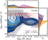 |
Fig. 1 Sub-samples extracted from the entire dataset of the SAM- CMASS mock galaxy catalogue, Gal-dens, as described in Table 1 and represented by coloured contours in the sSFR-M∗ parameter space at zref = 0.56. The number density distribution of the entire dataset is depicted as, logarithmically binned hexagons in the background. The horizontal solid red line marks the classic quiescent separation, log10(sSFR [yr]) ~ –11 (Franx et al. 2008). |
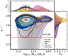 |
Fig. 2 Sub-samples extracted from the entire dataset of the SAM- CMASS mock galaxy catalogue, Gal-dens, as described in Table 1 and represented by coloured contours on the (g-i)-Mvir parameter space at zref = 0.56. The number density distribution of the entire dataset is depicted as grey, logarithmically binned hexagons in the background. The horizontal solid red line marks the classic separation of red and blue galaxies, (g-i) = 2.35 (Masters et al. 2011). |
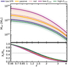 |
Fig. 3 Halo mass assembly history: in the upper panel we show the redshift evolution of median values of the halo mass, Mvir , according to the selection procedure outlined in Fig. B.1 for our five selected sub-samples: low-SFR (solid blue line with white dots indicating the redshift values of each snapshot), passive (solid light yellow line), red (short-dashed red line), low-Zcold (solid dark magenta line), and high- Zcold (dotted-dashed green line). The shaded regions represent the range spanning between the 32nd and the 68th percentile around the median. Their corresponding mass growth history relative to the reference redshift of our study, zref = 0.56, as z0 . In this panel, Xz denotes the values of Mvir at a specific snapshot/redshift compared to the values at z0 ( |

3 Results
We present results on the redshift evolution and assembly history of galaxy properties from modelled massive and luminous red galaxies using the CMASS mock galaxies from the semi- analytical model GALACTICUS. We apply selection criteria based on typical galaxy properties such as colour or star formation activity to select five sub-samples as discussed extensively in Section 2. We remind the reader that we use only central galaxies in our analysis.
3.1 Redshift evolution of galaxy and halo masses
In the upper panel of Fig. 3, we show the redshift evolution of the halo mass, Mvir7, for our five selected sub-samples: low- SFR (solid blue line with white dots indicating the redshift values of each snapshot), passive (solid light yellow line), red (short-dashed red line), low-Zcold (solid dark magenta line), and high-Zcold (dotted-dashed green line). In this figure and the following, we show median values of all galaxies present in each sub-sample along with the range spanning between the 32nd and the 68th percentile, shown as shaded coloured regions using the above-defined colour and line style keys. The lower panel of the same figure corresponds to their halo mass growth history  with Xz being the halo mass at a specific snap- shot/redshift and
  being the halo mass they hold at the reference redshift of our study zref = 0.56. The lower panel utilises the same colour scheme, line style keys, and statistical methods as in the upper panel.
Our results indicate that all defined sub-samples exhibit comparable evolutionary tracks but reach slightly different halo masses at zref The low-SFR and high-Zcold sub-samples, as well as passive and red sub-samples, show very well-aligned evolution, reaching the lowest (Mvir ~ 1013 M⊙) and intermediate (Mvir ~ 2 × 10¹³ M⊙) mass regimes, respectively. In contrast, low-Zcold galaxies are exceptions, acquiring significantly higher halo masses of around M200c ~ 1014 M⊙ compared to galaxies from the other four sub-samples. However, all galaxies still assemble half of their masses at similar redshifts between 1.2 < z < 1.4.
The redshift evolution of the stellar mass, M*, mirrors the trends observed for halo mass evolution; therefore, a separate plot is not provided. Instead, the following results are reported: aligned with results on the halo mass, the low-Zcold galaxies consist also of the most massive ones in stellar mass, which assemble half of their M* at z ~ 1.2, while low-SFR and high-Zcold galaxies already completed half of their mass assembly at z ~ 1.5. Furthermore, the low-Zcold (high-Zcold) galaxies show the highest (lowest) stellar-to-halo mass ratio, SHMR = M*/Mvir. Other sub-samples show intermediate values, with low-SFR-galaxies holding values comparable to high-Zcold galaxies, and red- and passive-galaxies values similar to low-Zcold. Interestingly, the evolution of the SHMR as a function of redshift peaks at z ~ 3.5 with SHMR ~ 0.01 for the low-SFR and high-Zcold samples. A similar peak can be found for the rest of the sub-samples but slightly later. Furthermore, from z ~ 1.5 to lower redshifts the SHMR evolution is almost constant across all sub-samples.
3.2 Redshift evolution of the cold gas and black hole masses
After examining the evolution of stellar and halo masses, the next step is to investigate the assembly histories of the corresponding cold gas, cold gas fraction (CGF), and central black hole masses. In Fig. 4 we show the redshift evolution of the cold gas mass, Mcold , which represents the gas available for conversion into stars. The steady growth in halo and stellar mass is supported by a consistently declining supply of Mcold and a decreasing cold gas fraction, CGF = Mcold/M*, towards later cosmic times for all sub-samples except low-Zcold . low-Zcold galaxies exhibit a constant CGF and maintain an extensive reservoir of cold gas. Notably, during their late-time evolution after z ~ 2, they were able to accumulate additional cold gas, resulting in a larger reservoir at lower redshifts compared to higher redshifts. This suggests that these galaxies are gaining additional fuel through their merger activity and smooth accretion from the cosmic web. This scenario is consistent with the evolution of their black hole masses, MBH, as shown in Fig. 5. In other words, the most massive galaxies also exhibit the highest MBH and possess the largest reservoir of Mcold to sustain their continued star formation. Conversely, galaxies with lower Mvir, M*, and MBH consume their cold gas at higher redshifts. These galaxies were among the first and fastest to assemble half of their stellar and black hole masses (see, e.g., the high-Zcold and low-SFR samples in the lower panel of Fig. 5). The following sections explore potential reasons for the significant difference in evolution observed in the Zcold sub-samples.
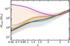 |
Fig. 4 Redshift evolution of median values of the cold gas mass, Mcold – the fraction of gas available to be converted into stars – for the different sub-samples. The figure utilises the same colour scheme, line style keys, and statistical methods as in Fig. 3. |
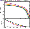 |
Fig. 5 Black hole mass assembly history: in the upper panel the redshift evolution of median values of the galaxy’s super-massive black hole, MBH is shown. The corresponding mass growth history relative to the reference redshift zref = 0.56 of our study, is displayed in the lower panel, following the same definitions as in Fig. 3. The figure utilises the same colour scheme, line style keys, and statistical methods as in Fig. 3. |
3.3 Redshift evolution of intrinsic galaxy properties
Until now, the discussion has centred on the assembly and growth history of mass-related properties. Here the focus shifts to additional properties such as star formation, metallicity, and colour. Therefore, we show in Fig. 6, from top to bottom, the redshift evolution is presented for: (a) the cold gas-phase metallicity, Zcold, (b) the observed SDSS colour (r-i), (c) the star formation rate, SFR, and (d) the star formation rate density, S FRD, normalised by the number of galaxies in each sub-sample at a particular redshift. Thin vertical dashed lines mark the redshifts z = [0.7,1.4,2.1,3.5], highlighting prominent features in the (r-i) colour evolution in panel b.
At low redshift, high-Zcold galaxies are the most metal enriched, as expected from their selection criteria. Galaxies of the low-SFR sample exhibit comparable metallicities to high-Zcold galaxies, while those in the red and passive samples show the second highest gas-phase metallicities. As anticipated, the low-Zcold galaxies are the least metal enriched at zref . Interestingly, at z ~ 2.5, this trend reverses, with low-Zcold galaxies becoming the most metal enriched, the highest Zcold. Moreover, the high-Zcold and low-SFR samples exhibit rapid metal production at higher redshift, as indicated by their steeper slopes in the Zcold evolution between 2 < z < 3 in panel a of Fig. 6, compared to the other sub-samples. After this period, the production rate slows down between z ∼ 2 and zref . In contrast, low-Zcold galaxies show a peak in Zcold between 2 ≲ z ≲ 3, followed by a continuous decline at later times.
In comparison to Zcold , we find little variation in the evolution of (r-i)-colour with cosmic time among our considered sub-samples, as shown in panel b of Fig. 6. The only exception is a short time interval of 1 ≲ z ≲ 1.5 where the low-SFR, passive, and red samples exhibit colours with (r-i) 0.25 redder than the low-Zcold and high-Zcold samples. This is puzzling, as their colour evolution is otherwise similar before and after this period. A similar behaviour in colour evolution has been suggested in another study using the same galaxy formation model (private communication with Tancara, in prep.). The cause of this gap between sub-samples is currently unclear, but Tancara et al. discuss this aspect in more detail in their upcoming work. Moreover, during this time interval, the colour evolution remains constant across all sub-samples. It is also noteworthy that the (ri) evolution demonstrates four prominent features, highlighted by vertical dashed lines: a maximum at z ~ 0.7, the edge of a constant colour evolution interval from 1 ≲ z ≲ 1.5 as mentioned above, and two minima at z ~ 2 and z ~ 3.5, respectively.
The first minimum in the colour evolution occurs around z ~ 3.5 as a short, rapid drop, followed by a prominent minimum at z ∼ 2 (panel b), coinciding with the “cosmic noon” – the peak of star formation in cosmic history (Madau & Dickinson 2014). During this period, all galaxies discussed in this study reached their bluest colours. Simultaneously, the low- Zcold sample shows a peak in Zcold (panel a). Interestingly, until z ~ 1.5, all galaxy samples exhibit the same median colour evolution and minima in both (r-i) and (g-i) colours. However, their median star formation rates (SFRs) differ, as shown in panel c. The low-Zcold, passive, and red samples display higher SFRs of approximately sim3–5 M⊙ yr−1 , compared to the lower rates seen in low-SFR and high-Zcold galaxies. After z ∼ 2, the galaxies undergo constant reddening until z ~ 1.5, followed by a period of no significant evolution until z ∼ 1. This epoch aligns with the time when half of the stellar and halo masses were assembled in all samples, except for low-Zcold . Furthermore, their corresponding mass growth functions reverse their curvatures – from growing more rapidly to more slowly – at this redshift (see the lower panel in Fig. 3).
At the last feature, a prominent peak in (r-i) at z ∼ 0.7, all galaxies reached their reddest colours in (r-i) independently of their sub-sample assignment. A similar evolution from bluer to redder colours until z ∼ 0.7 was also reported by Maraston et al. (2009) for modelled luminous red galaxies. In addition, the same peak can be observed in the (𝑔-i) colour at the same redshift for the low-Zcold and high-Zcold samples, while for the rest of the sub-samples, this peak occurs slightly earlier in cosmic time, at z ∼ 0.85.
The star formation rate density (SFRD), normalised by the galaxy number count (Ngal) in each sub-sample, is shown in the panel d of the same figure and does not indicate strong variations between the samples at cosmic noon. However, slightly higher SFRD/Ngal values are measured for the high-Zcold galaxies around z ∼ 1.5, coinciding with the edge of the no-evolution period in colour seen in panel b. This trend is also reflected in the specific star formation rate (sSFR), where high-Zcold galaxies consistently show higher, or at least similar, median sSFRs as other sub-samples at z > 0.85. Interestingly, the S FRD/Ngal of our sub-samples does not show the expected peak around cosmic noon. It is important to note that we normalised the SFRD by the comoving volume and the number of galaxies in each subsample to ensure an unbiased comparison across sub-samples. This results in lower values than the cosmic star formation rate density presented by Madau & Dickinson (2014). As shown in the figure, the curves for all sub-samples indicate a moderate increase in evolution at higher redshift. Unfortunately, our ability to explore this further is limited by the available merger tree data, which only tracks galaxies consistently up to z = 4.15. Nonetheless, an earlier peak in the cosmic star formation rate density8 of all galaxies in the GALACTICUS model, as shown in Fig. 4 of the THE MULTIDARK- GALAXIES release paper (Knebe et al. 2018b), between z ∼ 3–4 supports this hypothesis and may explain why we do not observe a peak at cosmic noon.
To summarise this section, our results indicate that low-Zcold galaxies consistently exhibit significantly higher M*, Mvir, as well as the largest black hole mass MBH in comparison to other sub-samples, including high-Zcold galaxies, as shown in Figs. 3– 5. These galaxies also accumulate large reservoirs of cold gas mass, Mcold , (unlike all other sub-samples) and terminate their evolution with more Mcold than they possessed initially at high redshift. Furthermore, they assemble their mass later and more rapidly, and produce stars more efficiently due to their abundant supply of Mcold compared to high-Zcold galaxies.
The high-Zcold galaxies, on the other hand, sit on the lower-mass end of the spectrum for Mvir, M∗ as well as MBH and therefore completed their mass assembly earlier and more continuously than their low-Zcold counterparts. This is reflected in their lower cold gas fraction in comparison to low-Zcold galaxies. In our companion paper S19 it was noted that there is a prominent bimodality in Zcold at the initial redshift of our study zref = 0.56. As discussed above, the authors could map this bimodality in low-Zcold and high-Zcold galaxies on specific galaxy and halo properties. We confirmed their hypothesis that high-Zcold and low-Zcold galaxies form via distinct pathways and correspond to two separate and distinguishable samples of galaxies that present the overall population of luminous and massive galaxies at zref. We aim at understanding what drives their distinct evolution via studying their clustering and location in the large-scale environment of the cosmic web.
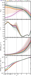 |
Fig. 6 From top to bottom, we present the redshift evolution of the following galaxy properties: (a) the cold gas-phase metallicity, Zcold ; (b) the observed colour, (r-i); (c) the star formation rate, SFR; and (d) the star formation rate density, SFRD, normalised by the number of galaxies in each sub-sample at a particular redshift. The vertical thin dashed lines mark redshifts of prominent line features in (r-i). The figure utilises the same colour scheme, line style keys, and statistical methods as in Fig. 3. |
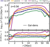 |
Fig. 7 Galaxy clustering functions: in the upper panel, we show the real- space two-point correlation function, ξ(r), at redshift zref = 0.56 for all sub-samples (using their respective colour scheme and line style keys as in Fig. 3) and the parent sample of the SAM-CMASS mock galaxies, Gal-dens (short-dashed black line). In the lower panel we display the fractional difference between the clustering function of each sub-sample (ξ(r)) and that of Gal-dens (ξ(r)ref). |
3.4 Galaxy clustering
In this section, we study the galaxy clustering of our different sub-samples of galaxies through the real-space two-point correlation function (2PCF), ξ(r). We use the CORRFUNC software package 9 from Sinha & Garrison (2017) and the standard Landy & Szalay (1993) estimator. We calculate 2PCFs with 25 logarithmic-spaced bins in the range of 0.5 < r (Mpc) < 150 assuming periodic boundary conditions. As stated previously, the galaxy samples have the same number density but different mean values for the stellar and halo masses, which is reflected in the clustering.
In the upper panel of Fig. 7 we show the 2PCF of central galaxies at redshift zref = 0.56 for all sub-samples (using the same colour and line style choices as in previous sections). We also include the result from the entire sample of SAM-CMASS mock galaxies, Gal-dens, as a reference (short-dashed black line). In the lower panel of the same figure, we plot the fractional difference of ξ(r) for each sub-sample with respect to the function of Gal-dens, ξ(r)ref.
As our results indicate, the low-SFR sample and the entire sample of SAM-CMASS mock galaxies, Gal-dens, have nearidentical correlation 2PCFs. This means that the 20% of low- starforming galaxies can mimic the clustering of the entire population of SAM-CMASS mock galaxies. As we previously described, Gal-dens is the parent sample from which all subsamples were extracted following a certain selection criterion listed in Table 1. This may largely be coincidental, as predictions for galaxy and halo properties from both the parent sample and the low-SFR sub-sample at zref as well as their subsequent evolution show no comparable trends.
Additionally, the clustering functions of our passive and red samples exhibit very similar 2PCFS, while low-Zcold galaxies show a significantly higher clustering amplitude. In contrast, the least clustered sample is high-Zcold, which displays the lowest amplitudes except for very small separations. A slight turnover in the clustering strength is observed at scales smaller than r < 2 Mpc, where high-Zcold (low-Zcold) galaxies cluster more (less) strongly. Interestingly, the low-Zcold and the high-Zcold samples represent the upper and lower limits in the total clustering strengths. These differences in the clustering are driven by the mean halo masses, with passive, red, and low-Zcold galaxies typically residing in the most massive and consequently the most clustered halos.
We also investigate the redshift evolution of the real-space clustering function, though we do not dedicate a separate plot to it, as the clustering strength shows only mild variation with redshift. Galaxies in the low-Zcold (high-Zcold) sample are always more (less) strongly clustered while the low-SFR sample shows an intermediate strength between low-Zcold and high-Zcold . As expected, these findings with the cosmic evolution of the halo masses of each galaxy sub-sample. At smaller separations, the clustering signal for low-Zcold galaxies decreases rapidly with increasing redshift, whereas low-SFR and high-Zcold galaxy pairs remain detectable at r < 2 Mpc or r < 5 Mpc at z = 0.7 or z = 3.51, respectively. Due to the given limitation in particle resolution and simulation box side-length, the 2PCFs exhibit growing uncertainties at larger separations.
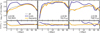 |
Fig. 8 Galaxy clustering functions in different environments: in the upper panels, we show the real-space two-point correlation function, ξ(r), at z = 0.56 for galaxies in the parent sample, Gal-dens (left panel), and for sub-samples low-Zcold (middle panel) and high-Zcold (right panel). In each panel we show the clustering for all galaxies in the sample (dashed black line), knot galaxies (solid yellow line), and filament galaxies (solid blue line with white dots). In the lower panel, we present the fractional difference in the clustering function of the filament and knot populations (ξ(r)), respectively, with respect to the clustering of the entire sample (‘all’, ξ(r)ref). |
3.5 Galaxy properties and the large-scale environment
We have shown that the low-Zcold and high-Zcold galaxy samples represent the upper and lower limits to the parameter space of various galaxy properties (see e.g. Figs. 1, 2, 3, or 5). In this section, we revisit our analysis by classifying the galaxies in our defined sub-samples according to their large-scale environmental affiliation of the cosmic web, categorised as “more-dense” or “less-dense” regions. To this extent, we apply the VWEB code (Hoffman et al. 2012; Libeskind et al. 2012, 2013; Carlesi et al. 2014; Cui et al. 2018, 2019) applying it to the dark matter catalogue that underpins our galaxy formation model. The code determines the environmental affiliation of the dark matter halos in which the galaxies reside according to “knots”, “filaments”, “sheets”, and “voids” as already discussed in our companion paper S19 (see Appendix A for details). In this analysis, we adopt the categories knots as “more-dense” and filaments as “less-dense” regions.
The upper panels of Fig. 8 show the 2PCF from left to right for Gal-dens, low-Zcold, and high-Zcold galaxies in knots (dark blue lines with white dots) and filaments (light yellow lines) as well as for all galaxies regardless of the environment (short-dashed black lines). The lower panels show the fractional difference between the knot and filament populations relative to the corresponding full sample. As expected, we observe a variation in clustering strength depending on separation length and large-scale environment, as demonstrated for the entire SAM- CMASS mock galaxy sample (left panel). Specifically, at smaller separations, r < 10 Mpc, knot galaxies (filament galaxies) cluster more (less) strongly, while at larger separations, the clustering strength becomes similar across both environments. The same behaviour is observed for high-Zcold galaxies up to r < 25 Mpc. However, unexpectedly, low-Zcold galaxies do not follow the same trend; instead, the clustering strength of knot, filament, and the overall population of low-Zcold galaxies is relatively similar. Notably, at the separation length of r ∼ 10 Mpc, we find a dip in the clustering for knot galaxies, but this feature is absent for filaments galaxies. Moreover, this dip is more pronounced in high-Zcold galaxies compared to low-Zcold ones.
To complement our galaxy clustering analysis, we compute the median values of the galaxy and halo properties for low-Zcold and high-Zcold galaxies in filaments and knots shown in Table 2. As previously reported by S19, we find a clear tendency for the halo mass, Mvir , to correlate with the environment. In more detail, the knot (filament) population of high-Zcold galaxies exhibits median halo masses within the 32nd and the 68th percentile of ![Mathematical equation: ${\log _{10}}\left( {{M_{{\rm{vir}}}}\left[ {{{\rm{M}}_ \odot }} \right]} \right) = 13.09_{ - 0.17}^{ + 0.17}\left( {{{\log }_{10}}\left( {{M_{{\rm{vir}}}}} \right.} \right.\left. {\left. {\left[ {{{\rm{M}}_ \odot }} \right]} \right) = 12.97_{ - 0.15}^{ + 0.15}} \right)$](/articles/aa/full_html/2025/01/aa49232-24/aa49232-24-eq6.png) compared to the low-Zcold galaxies of
compared to the low-Zcold galaxies of ![Mathematical equation: ${\log _{10}}\left( {{M_{{\rm{vir }}}}\left[ {{{\rm{M}}_ \odot }} \right]} \right) = 3.93_{ - 0.14}^{ + 0.15}\left( {{{\log }_{10}}\left( {{M_{{\rm{vir}}}}\left[ {{{\rm{M}}_ \odot }} \right]} \right) = 13.70_{ - 0.12}^{ + 0.14}} \right)$](/articles/aa/full_html/2025/01/aa49232-24/aa49232-24-eq7.png) , respectively. A visually demonstration and further description can be found in Fig. C.1 in Appendix C.
, respectively. A visually demonstration and further description can be found in Fig. C.1 in Appendix C.
As expected, low-Zcold galaxies have significantly higher halo masses and are predominantly located in knots (60%) and to a lesser extent in filaments (38%)10. This is in contrast to high-Zcold galaxies, which are primarily found in filaments (62%) while being found in knots to a lesser degree (24%)11.
For low-Zcold galaxies, we observe a clear environmental correlation where knot galaxies (compared to filament galaxies) possess larger (smaller) values for Mvir, M∗, MBH, and Tcons, but lower (higher) values for SFR, sSFR, and CNFW . Here, Tcons = Mcold/SFR/109 in Gyr is the cold gas consumption (or depletion) time, representing the efficiency with which the galaxy converts its cold gas into stars based on its current star formation rate, while CNFW denotes the concentration of the Navarro–Frenk–White dark matter halo profile as defined by Navarro et al. (1997). Notably, low-Zcold galaxies generally contain an order of magnitude more gas and metals in their hot halo (Mhot and  , respectively), as well as more metals in stars
  , but hold three orders of magnitude more cold gas (Mcold).
Furthermore, high-Zcold galaxies exhibit higher stellar-to- halo mass ratios (SHMR) and lower cold gas fractions, Mcold/M*, (s)SFRs. The cold gas consumption time for high- Zcold is approximately 0.5 Gyr for high-Zcold, while the measurement exceeds the age of the Universe multiple times. Interestingly, despite the fundamental differences in Zcold between the high-Zcold and low-Zcold sub-samples, both hold identical stellar metallicity values, Z∗ 12.
The black-hole-to-halo mass ratio, MBH/Mvir , also known as the black hole efficiency, a diagnostic tool that indicates how responsive a galaxy might be to AGN activity and how efficiently it can transport gas to its central region, which fuels the central black hole (see e.g. Ferrarese 2002; Croton 2009). The relation between MBH and Mvir is assumed to be tight and redshift dependent (as we discuss in the next section) (see e.g. Wyithe & Padmanabhan 2006; Booth & Schaye 2011), with their evolution being closely linked (see Powell et al. 2022, and the citations therein). We find that our considered sub-samples, as well as the parent sample, show similar values for MBH / Mvir , but with generally lower efficiencies in knots compared to filaments. Along with the colour indices, (ɡ-i) and (r-i), the stellar metallicity, Z*; these properties do not show a dependency with environment as demonstrated in Table 2.
A significant difference between low-Zcold and high-Zcold galaxies is observed in the mass of cold gas, Mcold , the cold gas fraction, Mcold/M*, the gas consumption time, Tcons, and the specific angular momentum of the baryons, jbar, being the sum of the angular momenta of the stellar spheroid and stellar disc components normalised by the sum of the total stellar and cold gas masses: jbar = (J*,disk + J*,bulge)/(M* + Mcold). Generally, we observe values for jbar ranging approximately between log10(jbar [kpckm s−1]) ~ 3–4, consistent with results from other models and observations Mancera Piña et al. (see e.g. 2021); Rodriguez-Gomez et al. (see e.g. 2022) for all sub-samples except low-Zcold . In addition, those galaxies also exhibit a slight environmental dependence: low-Zcold galaxies in knots exhibit higher jbar than those in filaments. Although the low-Zcold sample includes the most massive ones, their angular momenta, around log10 (jbar [k pckm s−1]) ~ 5, exceed the expected range based on the well-known power-law relation Fall (e.g. 1983); Romanowsky & Fall (e.g. 2012) by one order of magnitude. Furthermore, throughout their history, low-Zcold galaxies consistently exhibit higher angular momenta than other sub-samples; however, at z ~ 1.3, their momenta experience a significant boost. While the exact cause of this deviation remains uncertain, we speculate that merger events may be responsible for this outcome. It is noteworthy mentioning, that all of these properties are linked to the cold gas mass, which ultimately influences the cold gas-phase metallicity, Zcold , so these differences are expected.
Median values of galaxy and halo properties in large-scale environments.
3.6 Redshift evolution of knot and filament galaxies
We also tracked the redshift and assembly history of galaxies across different environments, presenting selected results for the parent sample, Gal-dens, as well as for the low-Zcold and high-Zcold sub-samples in this section. In the upper panels of the upper figure of Fig. 9, we present the assembly histories, and in the lower panels, the growth histories. In the left panel we plot the knot populations and in the right panel for the filament populations, respectively. We use the following colour and line style keys: short-dashed black lines for Gal-dens, solid magenta line with dots for low-Zcold , and dashed-dotted green line for high-Zcold.
We find that, in general, all filament populations exhibit flatter growth functions at lower redshift compared to the knot populations. Furthermore, 50% of the halo mass is assembled at z ≲ 1.2 (z ≳ 1.2) in low-Zcold galaxies (high-Zcold galaxies) located in knots. No significant difference is detected in the half-mass assembly times for the same sub-samples in filaments (refer to the vertical solid lines in the lower panels of the same figure, following the corresponding colour keys). Interestingly, stellar and black hole masses do not show a clear correlation with environment regarding their half-mass assembly time, as galaxies in both knots and filaments tend to assemble at similar redshifts.
low-Zcold galaxies generally exhibit greater sensitivity to their large-scale environment compared to high-Zcold galaxies, as demonstrated by the specific star formation rate (sSFR) in the lower figure of Fig. 9. The left (right) panel shows the sSFR evolution in knots (filaments) for the parent sample, Gal-dens, and the low-Zcold and high-Zcold sub-samples. We further highlight the classic star formation/quenching threshold being sSFR ∼ 10−11 yr−1 (Franx et al. 2008)13 as a horizontal solid red line. The vertical thin solid colour-coded lines mark the redshift where the sSFR drops below this threshold for low-Zcold galaxies (magenta) and high-Zcold galaxies (green). In general, low-Zcold galaxies enter passive evolution earlier than high-Zcold galaxies, and transitioning slightly earlier when located in the knots than in the filaments but typically at z ~ 1.1. In contrast, high-Zcold galaxies become passive later than their low-Zcold counterparts but approximately at the same redshift in knots and filaments, around z ~ 0.9. The drop below the threshold coincides with a decline in the SFRD as shown before in panel d of Fig. 6.
We analysed the evolution of all galaxy properties listed in Table 2. Properties such as Zcold , (r-i) colour-index, SFR, and SFRD exhibit only slight variations with respect to the environment. Therefore, we do not dedicate separate plots to it. The redshift evolution of Tcons reveals a turnover around z ~ 2.7, where high-Zcold galaxies initially consume their gas less efficiently than the low-Zcold galaxies. Around z ∼ 3, their consumption time suddenly drops below 0.2 Gyr and rises moderately to 0.5 Gyr with no notable dependence on the environment. Afterwards, the consumption time in low-Zcold galaxies rapidly surpasses 1 Gyr and eventually exceeds the age of the Universe after z ∼ 1. The parent sample, Gal-dens, occupies an intermediate stage between low-Zcold and high-Zcold sub-samples in terms of gas consumption evolution. All of these trends align with the evolution of the cold gas fraction, where the predictions differ between the sub-samples but show no environmental dependence.
The black hole efficiency, MBH/Mvir , reveals another turnover around z ∼ 3, where low-Zcold galaxies initially show a higher efficiency followed by high-Zcold galaxies. The former experiences a decline in efficiency between 1 < z < 2. We did not detect any significant difference between environments, although there is a general trend where knot galaxies exhibit higher efficiencies at first, followed by filament galaxies. Additionally, it is notable that high-Zcold galaxies became bulge- dominated much later (Mbulge/M* > 0.8 around z ~ 3) than low-Zcold galaxies.
3.7 Redshift evolution of galaxy clustering
To complete our result section, we show in Fig. 10 the clustering evolution of knot galaxies (upper panels) and filament galaxies (lower panels) of our selected sub-samples at various snapshots: z = [0.56,0.7,1.37,2.1,3.51], using the same line style and colour keys as in Fig. 9. For consistency, we chose zref and the same four redshift snapshots from left to right as indicated by the vertical lines in Fig. 6. In the two narrow panels, we show again the fractional difference of ξ(r) for each sub-sample relative to the function of Gal-dens, ξ(r)ref. As discussed previously, knot and filament populations exhibit different clustering behaviours. However, the evolution with redshift shows a mild trend towards lower clustering strength with increasing redshift. The shift of the separation length, r, where the 2PCFs drops to zero for the sub-samples low-Zcold and high-Zcold, is a consequence of the different median halo mass range sub-samples hold. high- Zcold galaxies are hosted by lower massive halos, which can be found in general at smaller separations than their low-Zcold counterparts.
It is also notable that the knot galaxies in the high-Zcold subsample generally exhibit higher clustering strength at smaller separations whereas their low-Zcold counterparts do so at higher separations. This leads to a turnover in the clustering strength in comparison to all galaxies between 5 ≲ r [Mpc] ≲ 10 (see narrow panels in the figure). Moreover, the redshift evolution of filament galaxies is markedly different: low-Zcold galaxies always cluster significantly stronger than the parent and high-Zcold samples. The high-Zcold galaxies, on the other hand, follow closely the clustering of Gal-dens.
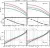 |
Fig. 9 Redshift evolution: in the upper figure, we present the redshift evolution or the median values of halo mass, Mvir , (upper panels) and the corresponding mass growth history, relative to the reference redshift of our study, zref = 0.56, (lower panels). Meanwhile, the lower figure illustrates the evolution of the specific star formation rate, sSFR. In both figures, the left panels display the evolution for knot environments, while the right panels show the corresponding evolution for filament environments. We include the parent sample, Gal-dens (short-dashed black line), alongside the low-Zcold (solid magenta line with white dots) and high-Zcold (dashed-dotted green line) sub-samples. The shaded regions represent the range between the 32nd and 68th percentiles around the median. In the upper figure, vertical solid lines mark the redshift at which 50% of the halo mass was assembled, known as the half-mass assembly time. In the lower figure, vertical solid lines indicate the redshifts where the low-Zcold (magenta) and high-Zcold (green) galaxies drop below the classic star formation/quenching threshold, sSFR ∼ 10−11 yr−1, as marked by the horizontal red line (Franx et al. 2008). Thin vertical black dashed lines highlight the redshifts of prominent line features in (r-i) shown in panel b of Fig. 6. |
4 Discussion and conclusions
The objective of this study was to investigate the redshift evolution and mass assembly history of sub-populations (subsamples of galaxies) selected from the same overall population of luminous and massive objects at z ~ 0.5. Thereby we employed a broad spectrum of properties and analysis strategies, including clustering functions and the galaxy-halo connection. In addition to examining the redshift evolution of galaxies within each sub-sample, we also distinguished them based on their location in the large-scale structure of the cosmic web, such as knots (denser regions) and filaments (less dense regions). This approach enabled us to explore their properties as well as the redshift evolution and assembly histories as a function of the environment. In this section, we discuss our findings and critically assess our conclusions.
4.1 Do the sub-samples studied in this work form via distinct formation channels?
We gathered significant evidence suggesting that the subsamples high-Zcold and low-Zcold form via distinct formation channels. We cannot confirm a similar conclusion for the rest of our sub-samples (low-SFR, red, and passive) since the galaxies in those sub-samples do not clearly map onto a prominent bimodality in the colour, sSFR, and Mvir spaces as shown in Figs. 1 and 2. The galaxies in these sub-samples are mixed populations, comprising galaxies from both peaks. Interestingly, the low-SFR sample shares evolutionary tracks with high-Zcold galaxies for nearly all galaxy properties (see e.g. Figs. 4 and 5), except for (r-i)-colour and CSFRD (see Fig. 6). As shown in Fig. 7, these sub-samples cluster very differently, likely due to the fact that they reside in dark matter halos of different masses. Furthermore, low-SFR galaxies can serve as a proxy for the overall 2-point correlation function for the entire sample of SAM-CMASS mock galaxies, Gal-dens (our parent sample). In addition, we find that the high-Zcold and low-Zcold sub-samples assembled half of their masses at different epochs (see Figs. 3, 5, and 9), exhibit distinct properties, primarily inhabit different environments (see Table 2 and Fig. 9), and ultimately cluster differently (see Figs. 7 and 8). Nonetheless, at intermediate redshifts, they share the same evolution of the colour parameter (r-i) as shown in panel b in Fig. 6.
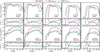 |
Fig. 10 Redshift evolution of the real-space 2PCF, ξ(r), for the selected sub-samples: Gal-dens, low-Zcold and high-Zcold, using the same colour and line style keys as described in Fig. 9. The uppermost panels display clustering for knot galaxies, while the lowermost panels show clustering for filament galaxies. Additionally, the fractional difference of ξ(r) with respect to the clustering of the parent samples, ξ(r)ref , is also presented. From left to right we include the initial redshift of sample selection, zref = 0.56, followed by the same four redshift snapshots marked by vertical lines in Fig. 6. |
4.2 To what degree are our results affected by the modelling itself?
Each semi-analytical model comes with its strengths and weaknesses, which have been discussed extensively by various authors over the years (see e.g. Knebe et al. 2015, 2018a). In this study, we leveraged the strengths of our adopted SAM, GALACTICUS, particularly its capabilities in modelling the galaxy-halo connection, luminosities, and the evolution of the cosmic star formation rate density (see Knebe et al. 2018b; Cui et al. 2019; Stoppacher et al. 2019). It could be argued that one of the main properties we focused on in this study, Zcold , is approximated in our model (see the definition in Section 2), as GALACTICUS does not provide the oxygen abundance directly but predicts only the cold gas mass and masses of metals. We find that the estimated values of Zcold align well with observational data, as demonstrated in the top panel of Fig. 7 in Knebe et al. (2018b). However, this figure also shows that GALACTICUS continues to exhibit a prominent bimodality in the cold gasphase metallicity until z ∼ 0.1 and an excess in metallicity beyond Zcold ∼ 9.5 at M* ∼ 1010.5 M⊙. We assume that this is, in fact, related to the implementation of the AGN-feedback, which directly affects cold gas-related properties as reported by the same authors. Several studies have reported that the implemented feedback strongly influences the resulting mass-metallicity relation across all redshifts (Torrey et al. 2014; De Rossi et al. 2017) while others report the opposite (Taylor & Kobayashi 2015; Thorne et al. 2022). Furthermore, the excess detected for our adopted model is relatively moderate within the considered stellar mass range M* > 1011 M⊙, where most of the SAM-CMASS mock galaxies can be found. Despite this, we cannot rule out the possibility that the metallicity bimodality in GALACTICUS is a peculiarity of this model. Nonetheless, recent works support the existence of such a bimodality and highlight the complexity of these properties in terms of galaxy evolution, morphology, and environment (e.g. Wotta et al. 2019; Donnan et al. 2022; Pistis et al. 2022; Omori & Takeuchi 2022).
4.3 What are the implications of our clustering results?
Fig. 8 reveals intriguing insights into the clustering of high- Zcold and low-Zcold galaxies based on their location within the cosmic web. high-Zcold galaxies in knots and filaments exhibit significantly different clustering patterns, despite residing in halos of similar mass14. Conversely, low-Zcold galaxies clustering behaviour in these environments, even though they inhabit halos of different masses. To ensure that these clustering behaviours are not merely a result of differences in stellar or halo masses, we selected four control samples: low (high) stellar mass as M*,low < 1011.3 M⊙(M*,high ≥ 1011.3 M⊙) and low (high) halo masses as Mhalo,low < 1013.6 M⊙ (Mhalo,high ≥ 1013.6 M⊙). We found that the assembly histories, redshift evolution, and clustering function of our control samples are different in comparison to those for low-Zcold and high-Zcold sub-samples reported in this work. In principle, the clustering results reported in Fig. 8 could potentially be related to the so-called “halo” and “galaxy assembly bias”, which are secondary dependencies of the halo bias at fixed halo mass manifested in the galaxy population (see e.g. Sheth & Tormen 2004; Gao et al. 2005; Wechsler et al. 2006; Yang et al. 2006; Croton et al. 2007). In Appendix C we conduct statistical tests on the similarity in halo mass distributions of filament and knot galaxies in high-Zcold. Further investigation will be devoted to addressing this specific connection.
4.4 Are our results in agreement with the fundamental metallicity relation (FMR)?
The FMR relates the gas-phase metallicity and stellar ages based on empirical calibrations of the oxygen-abundance, which in our case corresponds to the property of the cold gas-phase metal- licity, Zcold (Mannucci et al. 2010). In this framework, galaxies with higher Zcold have undergone stronger metal enrichment processes and are typically more massive. Interestingly, our results suggest the opposite: galaxies that are the most (least) massive exhibit lower (higher) values for Zcold . We emphasise that the prediction from GALACTICUS on Zcold is in agreement with the FMR. When comparing our results to those in the literature, all the galaxies considered in our sample low-Zcold and high- Zcold sub-samples are classified as “high metallicities” systems, with values of 12 + log10(O/H) > 8.5 (see the values for Zcold in Table 2). This corresponds, for example, to the high-metallicity predictions of Finlator & Davé (2008), Maiolino & Mannucci (2019), and Sánchez-Menguiano et al. (2019). Furthermore, the trend that galaxies in denser environments tend to exhibit slightly higher metallicities than those in less dense environments, as reported by studies such as Mouhcine et al. (2007) and Cooper et al. (2008), is consistent with our sample. In summary, two scenarios could help interpret the metal enrichment of cold gas in our results: “quenching by strangulation” for high-Zcold galaxies (e.g. Peng et al. 2015) and “metal-poor gas accretion” for low-Zcold galaxies (e.g. Ceverino et al. 2016).
The quenching by strangulation scenario is illustrated in Fig. 1 of Peng et al. (2015), and it explains well what we observed when studying the high-Zcold sub-sample: galaxies are cut off from continued gas accretion but can continue to form stars by recycling of the available enriched interstellar medium. As a consequence, their stellar mass and gas metallicity increase steeply due to the absence of dilution by inflowing metal-poor gas, a process commonly described as a “closed-box” model. The same authors predicted an upper stellar mass limit of M* ~ 1011 M⊙, beyond which this mechanism primarily drives quenching in local quiescent galaxies. Our high-Zcold galaxies fall within the uncertainty range, spanning from the 32nd to the 68th percentile around this threshold, as shown in Table 2. In addition, Trussler et al. (2020) found that the star-forming progenitors of local passive galaxies within the same mass range are principally quenched by starvation on a time-scale of 2 Gyr. However, they do not find the environmental trend that we report in this study.
The metal-poor gas accretion scenario describes the accretion of metal-poor gas from the intergalactic medium onto the galaxy. We expect that low-Zcold galaxies gain a significant amount of cold, metal-poor gas through recent gas-rich mergers (e.g. due to the incorporation of dwarf satellites) or directly from the intergalactic medium, which suppresses the metalenrichment process while boosting star formation Dekel et al. (2009b); van de Voort & Schaye (2012); Ceverino et al. (2016). This scenario was also been described by Dayal et al. (2013) using a simple analytical model. Furthermore, one or more “hot accretion”-events, likely occurring around massive structures, are also plausible (Sancisi et al. 2008). A similar prediction was made by Yates et al. (2012) also using a semi-analytical model. This scheme is further supported by the fact that the low-Zcold population showed higher net metallicity around z ∼ 2 compared to its final value at zref (see the top panel in Fig. 6). When considering the growth function of the cold gas reservoir and its metal masses (see Fig. 4), low-Zcold galaxies demonstrate a steady growth function from z = 1.5 to zref. These findings support our hypothesis that low-Zcold galaxies continue to be fuelled by cold gas at lower redshift, unlike high-Zcold galaxies, which primarily rely on their initial reservoir of Mcold for star formation. We also expect that low-Zcold galaxies harbour a younger stellar population compared to the high-Zcold sub-sample. Other authors have also suggested that cold streams could provide sufficient gas to sustain star formation in galaxies hosted by massive halos (Rodríguez-Puebla et al. 2017) and predicted that at redshifts z > 1, hot halos can be penetrated by these streams (see e.g. Kereš et al. 2005; Dekel & Birnboim 2006; Dekel et al. 2009a). Investigating the merger histories, particularly the distinction between minor and major mergers, would be a fruitful approach to further illuminate this matter.
4.5 Could the galaxies present in the low-Zcold sample be “ultra-luminous massive galaxies” (ULMGs)?
The progenitors of CMASS galaxies are known to be a passively evolving population of galaxies since z ~ 0.7. Although CMASS galaxies are frequently found in the centre of the most massive clusters and super-clusters (Lietzen et al. 2012), it remains unclear which galaxy population they might resemble at lower or higher redshift. ULMGs, believed to be the low-redshift progenitors of the most massive, passively evolving galaxies in the Universe (e.g. Cheema et al. 2020; Forrest et al. 2020), are either very massive and quiescent at z ~ 1.6 or a population of post-starburst galaxies that were quenched rapidly before z ∼ 3– 4. When compared to these studies, even galaxies in our most massive sample, low-Zcold, do not exhibit properties consistent with ULMGs, as both stellar and halo masses are still too low at the redshifts we consider. Our findings suggest that SAM- CMASS mock galaxies constitute a different population and follow an evolutionary path distinct from that of ultra-massive, early-quenched galaxies.
4.6 Does the mass-metallicity relation of our galaxy samples reveal different sub-types of “compact early-type galaxies” (cETGs)?
In their study of low-redshift cETGs, Kim et al. (2020) identified two environmentally dependent variants of the same population. One sub-population deviates from the classical mass-metallicity relation for early-type galaxies (Chilingarian & Zolotukhin 2015; Janz et al. 2016), suggesting the existence of different formation channels. Although we cannot directly compare our results to their findings due to differences in metallicity proxies, we observe similar trends in our data. Specifically, they found a higher-metallicity, lower-mass population primarily located in filaments, which aligns with the possibility that our high-Zcold population could evolve into cETGs at lower redshift. Furthermore, Borzyszkowski et al. (2017) introduced two populations of halos that have halo masses similar to those hosting our low- Zcold and high-Zcold galaxies. In a follow-up study, Romano-Díaz et al. (2017) discussed the detection of halo assembly bias, which resonates with our clustering results for the low-Zcold and high- Zcold populations across different environments. These findings further support a potential link between halo assembly bias and the formation of distinct galaxy sub-populations.
4.7 Why do we not compare our results to observations?
Comparing the redshift evolution of observation with data from models is generally challenging and involves significant modelling on the observational side. For instance, generating star formation histories for observed galaxies typically relies on “spectral energy distribution fitting” techniques available as computational packages (see e.g. Alarcon et al. 2023). These techniques depend on stellar synthesis population models such as developed by e.g. Conroy et al. (2009) or Vazdekis et al. (2010). Moreover, this work focuses on the intrinsic evolution of galaxies, which cannot be easily compared to observations since we cannot trace observed galaxies across time. Therefore, we chose not to include observational data in this work, as such a comparison would lack meaning. In a follow-up study, we will address the challenge of comparing to observations and how to generate the redshift evolution for observed galaxy populations of galaxies in more detail. We are working towards developing a complementary approach that involves tracking progenitors, inspired by observational data selection, and we will incorporate observational data for reference. This work is currently in preparation.
5 Summary and outlook
In this study, we have analysed the assembly history and redshift evolution of semi-analytically modelled massive and luminous red galaxies within the redshift range 0.5 ≲ z ≲ 4. In particular, we used the total population of the SAM-CMASS mock galaxy sample, Gal-dens, introduced and described in Stoppacher et al. (2019, referred to as S19), which replicates the selection of the well-studied observational BOSS-CMASS sample. Gal-dens served as our parent sample, and we extracted sub-samples from it based on typical selection criteria for galaxy properties using typical selection criteria based on galaxy properties at the initial redshift of our study zref = 0.56 (see Table 1). The galaxy properties we used for selection are (ɡ-i)-colour (red sub-sample), star formation activity (low-SFR and passive subsamples), and the cold gas-phase metallicity, Zcold (low-Zcold and high-Zcold sub-samples).
We subsequently tracked the progenitors of those galaxies that entered our defined sub-samples at zref to high redshift in order to reproduce the redshift evolution and growth histories starting at z = 4.15 to z = 0.56 (see illustration in Fig. B.1). In the first part of this work, we presented key properties, including halo masses ( Mvir, Fig. 3), stellar masses (M*), cold gas masses (Mcold, Fig. 4), black hole masses (MBH, Fig. 5), as well as the cold gas-phase metallicities (Zcold), the observed colours (r-i), the star formation rate (densities) (SFR and SFRD) in Fig. 6, and their clustering functions (Fig. 7). In the second part, we focused specifically on low-Zcold and high-Zcold sub-samples, examining their clustering functions (see Fig. 8) and evolutionary histories in different large-scale environments, such as knots (denser regions) and filaments (less dense regions), as detailed in Figs. 9, 10, and Table 2. We summarise our most important results in the following:
The galaxies in each sub-sample exhibit distinct median evolution trends for their galaxy and halo properties alongside varying as well as distinct growth and clustering functions. Notably, the most massive galaxies are the least metal enriched at z = 0.56. Members of the low-Zcold sub-sample consistently exhibit higher median values for M*, Mvir, and MBH. In contrast, galaxies with intermediate-to-lower masses for Mvir, M*, or MBH (corresponding to the passive, red, and high-Zcold sub-samples) tend to consume their cold gas at higher redshift. Furthermore, red and high-Zcold sub-samples are the earliest and quickest to assemble half of their M* and MBH . At higher and intermediate redshift, they exhibit lower Zcold, SFR, and CSFRD compared to other sub-samples (see Figs. 3–6).
We observe that the sub-samples low-Zcold and high-Zcold follow distinct evolutionary pathways and occupy different environments (see Table 2). Specifically, low-Zcold galaxies are predominantly found in denser regions such as knots (60%). Despite their later formation, they transition to passive evolution earlier than their high-Zcold counterparts. The high-Zcold galaxies mostly inhabit less dense regions such as filaments (62%). The high-Zcold filament and knot galaxies exhibit different clustering functions in both shape and amplitude, whereas the low-Zcold filament and knot populations show a similar clustering behaviour (see Fig. 8).
Furthermore, the redshift evolution and assembly histories of low-Zcold and high-Zcold galaxies are influenced by their environment. The high-Zcold galaxies formed half of their halo mass significantly earlier in knots compared to filaments (see upper figure in Fig. 9). In contrast, low-Zcold galaxies formed at essentially the same redshift in both environments. Regarding the quenching of star formation, high-Zcold galaxies generally transitioned to passive evolution later than low-Zcold galaxies in both environments. However, low-Zcold galaxies quenched slightly earlier in knots than in filaments (see lower figure in Fig. 9).
In this work, we have discussed, among other results, the evolution of galaxy properties using the progenitors of galaxies assigned to well-defined sub-samples at a particular redshift. Notably, this means that until now, we examined how the properties of galaxies, such as those that were the reddest or most metal enriched at zref , evolve over time. As shown in panel a of Fig. 6, galaxies meeting a specific selection criterion at zref (in this case low or high cold gas-phase metallicity, Zcold) do not necessarily maintain that criterion throughout their redshift evolution. This is expected and reflected in almost all galaxy properties, as they undergo substantial evolution and change during their assembly history. In addition, in this particular study, we have- focused on the intrinsic evolution of galaxies throughout cosmic history, which provides valuable insights into the true evolution of a given galaxy population. As noted in the discussion section, understanding this intrinsic evolution is crucial. Moving forward, we aim to develop a complementary approach that integrates observational data to trace redshift evolution. This will enhance our ability to compare predictions from models with observations, which is increasingly relevant given the extensive sky surveys from recent and upcoming observational missions.
Acknowledgements
We thank the anonymous referee for their constructive and insightful comments, which have significantly improved the quality of this article. DS is funded by the Spanish Ministry of Universities and the European Next Generation Fond under the Margarita Salas Fellowship CA1/RSUE/2021-00720. DS also wants to thank Brant Robertson for granting her time to work on this project and José Oñorbe for his guidance and support on bureaucratic issues as well as as the team from Koblischek-byKatrin for serving excellent coffee in an amazing atmosphere in Weiz and further Dr. Rosa Maria Laβnig for her kind and professional support during the last years. The CoSMoSlM-database used in this paper is a service by the Leibniz-Institute for Astrophysics Potsdam (AIP). The MultiDark database was developed in cooperation with the Spanish MultiDark Consolider Project CSD2009-00064. In addition, this work has benefited from the publicly available software tools and packages: MATPLOTLIB (Hunter 2007); Python Software Foundation (https://www.python.org) 1990-2023, version 2.7 and 3; ANACONDA (https://www.anaconda.com); PYENV (https://github.com/pyenv/pyenv); SEABORN (https://seaborn.pydata.org/) and STATSMODELS (Seabold & Perktold 2010); ASTROPY (https://www.astropy.org/) (Astropy Collaboration 2013, 2018); JUPYTER NOTEBOOK (https://jupyter-notebook.readthedocs.io/en/latest/); The CentOS Project (https://www.centos.org), The Fedora Project (https://fedoraproject.org/), TOPCAT (Taylor 2013). We used openAI’s GPT-4 lan-guage model for assistance with language refinement and drafting parts of the manuscript. ADMD thanks Fondecyt for financial support through the Fonde-cyt Regular 2021 grant 1210612. AK is supported by the Ministerio de Ciencia e Innovación (MICINN), Spain under research grant PID2021-122603NB-C21 and further thanks The Me In You for girl in amour. NDP acknowledges support from a RAICES grant from the Ministerio de Ciencia, Tecnología e Innovación, Argentina.
Appendix A Information on the adopted galaxy catalogue: MDPL2-Galacticus
As GALACTICUS is primarily described in Benson (2012), with additional features outlined in Knebe et al. (Sec. 2.2 and Tab. 1 2018b) as part of the THE MULTIDARK-GALAXIES catalogues, we summarise only its aspects most relevant to this work. The GALACTICUS semi-analytic model incorporates a stellar population synthesis model from Conroy et al. (2009), an initial mass function from Chabrier (2003), and a dust model of Ferrara et al. (1999). The definition of the dark matter halo mass is given by
 (A.1)
(A.1)
where Δref = ΔBN98 for MBN98 with ΔBN98 being the virial factor as given by the Eq. (6) of Bryan & Norman (1998); ρc denotes the critical density of the Universe, and Rref is the corresponding halo radius at which the interior mean density matches the desired value as specified on the right-hand side of Eq. (A.1). We note that ROCKSTAR offers various halo mass definitions; however, this version of GALACTICUS was run using this one.
The parameters for galaxy formation physics in GALACTICUS were determined through a manual search of the parameter space, aiming to match a variety of observational data. These include the ɀ = 0 stellar mass function of galaxies (Li & White 2009), ɀ = 0 K and bJ-band luminosity functions (Cole et al. 2001; Norberg et al. 2002), the local Tully-Fisher relation (Piza-gno et al. 2007), the colour-magnitude distribution of galaxies in the local Universe (Weinmann et al. 2006), the distribution of disc sizes at ɀ = 0 (de Jong & Lacey 2000), the black hole mass to bulge mass relation (Häring & Rix 2004), and the star formation history of the Universe (Hopkins et al. 2014).
This version of GALACTICUS employs a simple accretion model where gas accretes from the intergalactic medium onto the dark matter halo, as outlined by Benson et al. (Eq. (35) in 2002). Cooling rates from the hot halo are computed using the traditional cooling radius approach from White & Frenk (1991). Metallicity-dependent cooling curves are calculated with CLOUDY (v13.01, Ferland et al. 2013). The disc is modelled as either a radiatively efficient, geometrically thin, Shakura & Sun-yaev (1973)-type disc (if the accretion rate being between 0.01 and  , where
  being the Eddington accretion rate) or otherwise as an advection-dominated flow-accretion thick disc, following (Begelman 2014). The model dynamically switches between these two modes.
Star formation is modelled using the prescription of Krumholz et al. (2009, i.e. their Eq. (1) for the star formation rate surface density, and Eq. (2) for the molecular fraction), assuming that the cold gas of each galaxy follows an exponential radial distribution. The scale length of this distribution is determined from the disc’s angular momentum by solving for the equilibrium radius within the gravitational potential of the disc+bulge+dark matter halo system (Gnedin et al. 2004). Metal enrichment is tracked using the instantaneous recycling approximation, with a recycled fraction of 0.46 and yield of 0.035. Metals are assumed to be fully mixed in all phases, thereby tracing all mass flows between phases.
The supernova feedback is implemented using a wind mass loading factor, β, computed as β = (Vdisc/250km/s)−3.5 where Vdisc is the circular velocity at the disc’s scale radius. Gas expelled from the galaxy by winds is retained in a reservoir for outflowed gas, which gradually leaks mass back into the hot halo on a timescale of tdyn/5, where tdyn is the dynamical time of the halo at the virial radius. Material is transferred from the disc to the spheroid on an instability timescale, which is defined by an instability parameter as described in Efstathiou et al. (1982) (see also Eq. (1) in Knebe et al. 2018b).
GALACTICUS does not include a specific starburst mode. Instead, star formation in the spheroid occurs at a rate Ṁ★ = 0.04Mgas/tdyn(V/200km/s)−2, where tdyn is the dynamical time of the spheroid at its half mass radius, and V its circular velocity at the same radius. The model tracks the mass and spin of black holes in detail, assuming an initial seed mass of 100 M⊙. AGN feedback is incorporated in both the “radio” mode (see Benson & Bower 2010) and the “quasar” mode (see Ostriker et al. 2010) with a black hole wind efficiency of 0.0024 being implemented. The model uses the standard spheroid implementation adopting a spheroid density profile (Hernquist-profile (Hernquist 1990)), which is described by a single-length scale where stars trace the gas density.
If the (baryonic) mass ratio of two merging galaxies exceeds 1:4, a ”major“ merger is assumed. In this scenario, the merging galaxies are transformed into a spheroidal remnant. Otherwise, a “minor” merger occurs, where the less massive galaxy is incorporated into the spheroid of the more massive galaxy, leaving the disc of the larger galaxy unaffected.
Appendix B Tracing modelled galaxies across cosmic history
Fig. B.1 provides a schematic representation of the selection procedure and tracking of progenitor halos. This is achieved by using the unique identification numbers – parentlndex – of central dark matter halos hosting the galaxy of interest to trace their main progenitor halos on their merger trees back in time. This information is provided by the halo finder and the corresponding tree builder algorithm. By definition, the merger tree main branch of the algorithm applied to the data used in this study (e.g. ROCKSTAR and CONSISTENT TREES), is the most massive progenitor branch and can be traced on the leftmost side of each sub-tree – the lowest mainLeafId – in the friend-of-friends (FoF) groups. That means in practice that the main progenitor halo, the one of interest, always has the lowest ID (denoted by the satelliteNodeIndex) for the same parentIndex and is also the most massive progenitor. That is particularly useful given that the MDPL2-Galacticus catalogue includes millions of galaxies and satellite galaxies that need to be filtered and traced to find the specific one of interest. It is important to note that while the GALACTICUS model uses the same IDs, it employs a different naming convention that may not be immediately recognisable to those familiar with ROCKSTAR terminology. For additional information, readers are referred to the COSMOSIM-database.
It is noted that while it may seem excessive to dedicate an additional figure solely to the tracking of progenitor halos, the companion paper in preparation will demonstrate that the sub-sample selection procedure does not necessarily need to be conducted at a specific redshift. This flexibility will lead to a different approach for target selection.
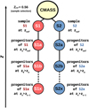 |
Fig. B.1 Schematic representation of the selection procedure and tracking of progenitor halos. The selection criteria were applied only once at the ɀref = 0.56, resulting in the S1 and S2 from the entire population of CMASS mock galaxies catalogue. The progenitors of these samples are then identified at the subsequent simulation snapshot using their unique identification number, resulting in the progenitor sub-samples Sla corresponding to S1-sample and S2a to S2-sample. This step is repeated and we subsequently move towards higher redshifts (S1x and S2x). This process is repeated as we progress to higher redshifts, generating S1x and S2x. This approach represents the conventional method for extracting information on the redshift evolution of galaxies in simulations. |
Appendix C Illustration halo mass dependency on environment
In this appendix, we illustrate and assess the statistical similarity of galaxies in the low-Zcold and high-Zcold sub-samples based on their large-scale environments (filaments or knots). As shown in Fig. 8 high-Zcold filament and knot galaxies exhibit distinct clustering functions, even though the median halo masses for these galaxies differ by only 0.13 dex in M⊙. Conversely, the median halo masses for low-Zcold filament and knot galaxies are separated by 0.23 dex in M⊙, yet they show similar clustering functions in both shape and amplitude at ɀ = 0.56. In Fig. C.1, we present violin plots showing the distribution of halo mass (Mvir) for high-Zcold and low-Zcold galaxies, with overlaid box plots in grey. This plot visually confirms that the knot population (displayed in blue by the left half of the violin) and the filament population (shown in yellow by the right half of the violin) behave consistently with the findings from the clustering analysis.
Their median values are more spread out, closer to the edges of the interquartile range. high-Zcold galaxies, on the other hand, have median values that are more closely aligned. Although the median halo masses of high-Zcold galaxies in both knots and filaments are similar, their clustering behaviour differs (Fig. 8). Conversely, low-Zcold galaxies cluster similarly in both knots and filaments, despite their statistical distributions differing. To support these observations, we conducted a Kolmogorov-Smirnov (KS) test using the Python package SciPy. stats to compare the filament and knot populations in both sub-samples.
The KS test is a robust method to assess whether their distributions are statistically similar. The KS statistic outputs a value between zero and one, which represents the maximum distance between the cumulative distribution functions (CDFs) of the compared samples. The KS statistic values closer to zero indicate that the distributions are more similar, while values closer to one suggest greater divergence between the distributions. For the high-Zcold sample, the KS test returned a value of 0.15 (with a p-value < 0.0515) when comparing filament and knot galaxies. This result indicates that the two distributions are relatively similar, with a moderate difference of 0.15 between their CDFs. In the low-Zcold sub-sample, the KS test returned a value of 0.3, double that of the high-Zcold sample. This larger value signifies a greater discrepancy between the distributions, meaning they are less similar. We also conducted similar tests in narrow halo mass bins and found consistent results.
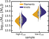 |
Fig. C.1 Violin plot visualising the distribution of halo mass (Mvir) for the sample. The high-Zcold galaxies are shown on the left, and the low-Zcold galaxies are on the right. Each violin displays the distribution of filament and knot galaxies. The left side of each violin represents the filament galaxy distribution, while the right side shows the knot galaxy distribution. We have also overlayed box plots in grey, with the median values marked in white. This visual representation confirms the results of our KS test: filament and knot galaxies in the high-Zcold sub-sample are statistically closer, while filament and knot galaxies in the low-Zcold exhibit greater differences. |
References
- Alam, S., Albareti, F. D., Allende Prieto, C., et al. 2015, ApJS, 219, 12 [Google Scholar]
- Alarcon, A., Hearin, A. P., Becker, M. R., & Chaves-Montero, J. 2023, MNRAS, 518, 562 [Google Scholar]
- Allende Prieto, C., Lambert, D. L., & Asplund, M. 2001, ApJ, 556, L63 [Google Scholar]
- Argudo-Fernández, M., Lacerna, I., & Duarte Puertas, S. 2018, A&A, 620, A113 [NASA ADS] [CrossRef] [EDP Sciences] [Google Scholar]
- Asplund, M., Grevesse, N., Sauval, A. J., & Scott, P. 2009, ARA&A, 47, 481 [NASA ADS] [CrossRef] [Google Scholar]
- Astropy Collaboration (Robitaille, T. P., et al.) 2013, A&A, 558, A33 [NASA ADS] [CrossRef] [EDP Sciences] [Google Scholar]
- Astropy Collaboration (Price-Whelan, A. M., et al.) 2018, AJ, 156, 123 [Google Scholar]
- Baugh, C. M. 2006, Rep. Prog. Phys., 69, 3101 [NASA ADS] [CrossRef] [Google Scholar]
- Baugh, C. M. 2013, in The Intriguing Life of Massive Galaxies, 295, 191 [NASA ADS] [Google Scholar]
- Begelman, M. C. 2014, arXiv e-prints [arXiv:1410.8132] [Google Scholar]
- Behroozi, P. S., Wechsler, R. H., & Wu, H.-Y. 2013a, ApJ, 762, 109 [NASA ADS] [CrossRef] [Google Scholar]
- Behroozi, P. S., Wechsler, R. H., Wu, H.-Y., et al. 2013b, ApJ, 763, 18 [NASA ADS] [CrossRef] [Google Scholar]
- Benson, A. J. 2010, Phys. Rep., 495, 33 [NASA ADS] [CrossRef] [Google Scholar]
- Benson, A. J. 2012, New A, 17, 175 [NASA ADS] [CrossRef] [Google Scholar]
- Benson, A. J., & Bower, R. 2010, MNRAS, 405, 1573 [NASA ADS] [Google Scholar]
- Benson, A. J., Frenk, C. S., Lacey, C. G., Baugh, C. M., & Cole, S. 2002, MNRAS, 333, 177 [NASA ADS] [CrossRef] [Google Scholar]
- Blanton, M. R., & Berlind, A. A. 2007, ApJ, 664, 791 [NASA ADS] [CrossRef] [Google Scholar]
- Booth, C. M., & Schaye, J. 2011, MNRAS, 413, 1158 [NASA ADS] [CrossRef] [Google Scholar]
- Borzyszkowski, M., Porciani, C., Romano-Díaz, E., & Garaldi, E. 2017, MNRAS, 469, 594 [NASA ADS] [CrossRef] [Google Scholar]
- Bose, S., & Loeb, A. 2021, ApJ, 912, 114 [NASA ADS] [CrossRef] [Google Scholar]
- Bryan, G. L., & Norman, M. L. 1998, ApJ, 495, 80 [NASA ADS] [CrossRef] [Google Scholar]
- Carlesi, E., Knebe, A., Lewis, G. F., Wales, S., & Yepes, G. 2014, MNRAS, 439, 2943 [NASA ADS] [CrossRef] [Google Scholar]
- Ceverino, D., Sánchez Almeida, J., Muñoz Tuñón, C., et al. 2016, MNRAS, 457, 2605 [NASA ADS] [CrossRef] [Google Scholar]
- Chabrier, G. 2003, PASP, 115, 763 [Google Scholar]
- Cheema, G. K., Sawicki, M., Arcila-Osejo, L., et al. 2020, MNRAS, 494, 804 [NASA ADS] [CrossRef] [Google Scholar]
- Chilingarian, I., & Zolotukhin, I. 2015, Science, 348, 418 [NASA ADS] [CrossRef] [Google Scholar]
- Chuang, C.-H., Prada, F., Pellejero-Ibanez, M., et al. 2016, MNRAS, 461, 3781 [CrossRef] [Google Scholar]
- Cole, S., Norberg, P., Baugh, C. M., et al. 2001, MNRAS, 326, 255 [NASA ADS] [CrossRef] [Google Scholar]
- Conroy, C. 2013, ARA&A, 51, 393 [NASA ADS] [CrossRef] [Google Scholar]
- Conroy, C., Gunn, J. E., & White, M. 2009, ApJ, 699, 486 [Google Scholar]
- Conselice, C. J. 2014, ARA&A, 52, 291 [CrossRef] [Google Scholar]
- Contini, E., Gu, Q., Ge, X., et al. 2020, ApJ, 889, 156 [NASA ADS] [CrossRef] [Google Scholar]
- Cooper, M. C., Tremonti, C. A., Newman, J. A., & Zabludoff, A. I. 2008, MNRAS, 390, 245 [NASA ADS] [CrossRef] [Google Scholar]
- Costantin, L., Pérez-González, P. G., Méndez-Abreu, J., et al. 2021, ApJ, 913, 125 [NASA ADS] [CrossRef] [Google Scholar]
- Croton, D. J. 2009, MNRAS, 394, 1109 [NASA ADS] [CrossRef] [Google Scholar]
- Croton, D. J. 2013, PASA, 30, e052 [NASA ADS] [CrossRef] [Google Scholar]
- Croton, D. J., Springel, V., White, S. D. M., et al. 2006, MNRAS, 365, 11 [Google Scholar]
- Croton, D. J., Gao, L., & White, S. D. M. 2007, MNRAS, 374, 1303 [Google Scholar]
- Cuesta, A. J., Vargas-Magaña, M., Beutler, F., et al. 2016, MNRAS, 457, 1770 [Google Scholar]
- Cui, W., Knebe, A., Yepes, G., et al. 2018, MNRAS, 473, 68 [NASA ADS] [CrossRef] [Google Scholar]
- Cui, W., Knebe, A., Libeskind, N. I., et al. 2019, MNRAS, 485, 2367 [Google Scholar]
- Davé, R., Crain, R. A., Stevens, A. R. H., et al. 2020, MNRAS, 497, 146 [Google Scholar]
- Davies, J. J., Crain, R. A., & Pontzen, A. 2021, MNRAS, 501, 236 [Google Scholar]
- Dayal, P., Ferrara, A., & Dunlop, J. S. 2013, MNRAS, 430, 2891 [Google Scholar]
- de Jong, R. S., & Lacey, C. 2000, ApJ, 545, 781 [NASA ADS] [CrossRef] [Google Scholar]
- Dekel, A., & Birnboim, Y. 2006, MNRAS, 368, 2 [NASA ADS] [CrossRef] [Google Scholar]
- Dekel, A., Birnboim, Y., Engel, G., et al. 2009a, Nature, 457, 451 [Google Scholar]
- Dekel, A., Sari, R., & Ceverino, D. 2009b, ApJ, 703, 785 [Google Scholar]
- De Lucia, G., Springel, V., White, S. D. M., Croton, D., & Kauffmann, G. 2006, MNRAS, 366, 499 [NASA ADS] [CrossRef] [Google Scholar]
- De Rossi, M. E., Bower, R. G., Font, A. S., Schaye, J., & Theuns, T. 2017, MNRAS, 472, 3354 [Google Scholar]
- Dolfi, A., Gómez, F. A., Monachesi, A., et al. 2023, MNRAS, 526, 567 [NASA ADS] [CrossRef] [Google Scholar]
- Donnan, C. T., Tojeiro, R., & Kraljic, K. 2022, Nature, 6, 599 [NASA ADS] [Google Scholar]
- Dressler, A. 1980, ApJ, 236, 351 [Google Scholar]
- Dutta, R., Fumagalli, M., Fossati, M., et al. 2020, MNRAS, 499, 5022 [CrossRef] [Google Scholar]
- Efstathiou, G., & Rees, M. J. 1988, MNRAS, 230, 5 [Google Scholar]
- Efstathiou, G., Lake, G., & Negroponte, J. 1982, MNRAS, 199, 1069 [NASA ADS] [CrossRef] [Google Scholar]
- Eisenstein, D. J., Weinberg, D. H., Agol, E., et al. 2011, AJ, 142, 72 [Google Scholar]
- Fall, S. M. 1983, in IAU Symposium, Vol. 100, Internal Kinematics and Dynamics of Galaxies, ed. E. Athanassoula, 391 [NASA ADS] [CrossRef] [Google Scholar]
- Favole, G., McBride, C. K., Eisenstein, D. J., et al. 2016, MNRAS, 462, 2218 [NASA ADS] [CrossRef] [Google Scholar]
- Ferland, G. J., Porter, R. L., van Hoof, P. A. M., et al. 2013, Rev. Mexicana Astron. Astrofis., 49, 137 [Google Scholar]
- Ferrara, A., Bianchi, S., Cimatti, A., & Giovanardi, C. 1999, ApJS, 123, 437 [CrossRef] [Google Scholar]
- Ferrarese, L. 2002, ApJ, 578, 90 [NASA ADS] [CrossRef] [Google Scholar]
- Filho, M. E., Sánchez Almeida, J., Muñoz-Tuñón, C., et al. 2015, ApJ, 802, 82 [NASA ADS] [CrossRef] [Google Scholar]
- Finlator, K., & Davé, R. 2008, MNRAS, 385, 2181 [NASA ADS] [CrossRef] [Google Scholar]
- Forrest, B., Marsan, Z. C., Annunziatella, M., et al. 2020, ApJ, 903, 47 [NASA ADS] [CrossRef] [Google Scholar]
- Franx, M., van Dokkum, P. G., Förster Schreiber, N. M., et al. 2008, ApJ, 688, 770 [NASA ADS] [CrossRef] [Google Scholar]
- Fukugita, M., Ichikawa, T., Gunn, J. E., et al. 1996, AJ, 111, 1748 [Google Scholar]
- Gao, L., Springel, V., & White, S. D. M. 2005, MNRAS, 363, L66 [NASA ADS] [CrossRef] [Google Scholar]
- Gnedin, O. Y., Kravtsov, A. V., Klypin, A. A., & Nagai, D. 2004, ApJ, 616, 16 [Google Scholar]
- Guo, H., Yang, X., & Lu, Y. 2018, ApJ, 858, 30 [NASA ADS] [CrossRef] [Google Scholar]
- Gupta, A., Tran, K.-V., Cohn, J., et al. 2020, ApJ, 893, 23 [NASA ADS] [CrossRef] [Google Scholar]
- Harada, N., Yajima, H., & Abe, M. 2023, MNRAS, 525, 5868 [NASA ADS] [CrossRef] [Google Scholar]
- Häring, N., & Rix, H.-W. 2004, ApJ, 604, L89 [Google Scholar]
- Hashemizadeh, A., Driver, S. P., Davies, L. J. M., et al. 2021, MNRAS, 505, 136 [NASA ADS] [CrossRef] [Google Scholar]
- Hawarden, T. G., van Woerden, H., Mebold, U., Goss, W. M., & Peterson, B. A. 1979, A&A, 76, 230 [NASA ADS] [Google Scholar]
- Hernquist, L. 1990, ApJ, 356, 359 [Google Scholar]
- Hoffman, Y., Metuki, O., Yepes, G., et al. 2012, MNRAS, 425, 2049 [Google Scholar]
- Hopkins, P. F., Kereš, D., Oñorbe, J., et al. 2014, MNRAS, 445, 581 [NASA ADS] [CrossRef] [Google Scholar]
- Hubble, E. P. 1936, Realm of the Nebulae (New Haven: Yale University Press) [Google Scholar]
- Hughes, T. M., Cortese, L., Boselli, A., Gavazzi, G., & Davies, J. I. 2013, A&A, 550, A115 [NASA ADS] [CrossRef] [EDP Sciences] [Google Scholar]
- Hunter, J. D. 2007, Comput. Sci. Eng., 9, 90 [NASA ADS] [CrossRef] [Google Scholar]
- Inagaki, T., Lin, Y.-T., Huang, H.-J., Hsieh, B.-C., & Sugiyama, N. 2015, MNRAS, 446, 1107 [NASA ADS] [CrossRef] [Google Scholar]
- Janz, J., Norris, M. A., Forbes, D. A., et al. 2016, MNRAS, 456, 617 [NASA ADS] [CrossRef] [Google Scholar]
- Johnston, E. J., Häußler, B., Jegatheesan, K., et al. 2022, MNRAS, 514, 6141 [NASA ADS] [CrossRef] [Google Scholar]
- Kaiser, N. 1984, ApJ, 284, L9 [NASA ADS] [CrossRef] [Google Scholar]
- Kalinova, V., Colombo, D., Sánchez, S. F., et al. 2021, A&A, 648, A64 [NASA ADS] [CrossRef] [EDP Sciences] [Google Scholar]
- Kereš, D., Katz, N., Weinberg, D. H., & Davé, R. 2005, MNRAS, 363, 2 [Google Scholar]
- Kim, S., Jeong, H., Rey, S.-C., et al. 2020, ApJ, 903, 65 [NASA ADS] [CrossRef] [Google Scholar]
- Klypin, A., Yepes, G., Gottlöber, S., Prada, F., & Heß, S. 2016, MNRAS, 457, 4340 [Google Scholar]
- Knebe, A., Pearce, F. R., Thomas, P. A., et al. 2015, MNRAS, 451, 4029 [CrossRef] [Google Scholar]
- Knebe, A., Pearce, F. R., Gonzalez-Perez, V., et al. 2018a, MNRAS, 475, 2936 [NASA ADS] [CrossRef] [Google Scholar]
- Knebe, A., Stoppacher, D., Prada, F., et al. 2018b, MNRAS, 474, 5206 [Google Scholar]
- Kormendy, J. 1979, ApJ, 227, 714 [Google Scholar]
- Koyama, Y., Smail, I., Kurk, J., et al. 2013, MNRAS, 434, 423 [CrossRef] [Google Scholar]
- Krajnović, D., Ural, U., Kuntschner, H., et al. 2020, A&A, 635, A129 [NASA ADS] [CrossRef] [EDP Sciences] [Google Scholar]
- Krumholz, M. R., McKee, C. F., & Tumlinson, J. 2009, ApJ, 699, 850 [NASA ADS] [CrossRef] [Google Scholar]
- Lackner, C. N., Cen, R., Ostriker, J. P., & Joung, M. R. 2012, MNRAS, 425, 641 [NASA ADS] [CrossRef] [Google Scholar]
- Landy, S. D., & Szalay, A. S. 1993, ApJ, 412, 64 [Google Scholar]
- Li, C., & White, S. D. M. 2009, MNRAS, 398, 2177 [NASA ADS] [CrossRef] [Google Scholar]
- Libeskind, N. I., Hoffman, Y., Knebe, A., et al. 2012, MNRAS, 421, L137 [NASA ADS] [CrossRef] [Google Scholar]
- Libeskind, N. I., Hoffman, Y., Forero-Romero, J., et al. 2013, MNRAS, 428, 2489 [NASA ADS] [CrossRef] [Google Scholar]
- Lietzen, H., Tempel, E., Heinämäki, P., et al. 2012, A&A, 545, A104 [NASA ADS] [CrossRef] [EDP Sciences] [Google Scholar]
- Lin, Y.-T., Mandelbaum, R., Huang, Y.-H., et al. 2016, ApJ, 819, 119 [NASA ADS] [CrossRef] [Google Scholar]
- Liu, G. C., Lu, Y. J., Xie, L. Z., Chen, X. L., & Zhao, Y. H. 2016, A&A, 585, A52 [NASA ADS] [CrossRef] [EDP Sciences] [Google Scholar]
- Luparello, H. E., Lares, M., Paz, D., et al. 2015, MNRAS, 448, 1483 [CrossRef] [Google Scholar]
- Lutz, K. A., Kilborn, V., Catinella, B., et al. 2020, A&A, 635, A69 [NASA ADS] [CrossRef] [EDP Sciences] [Google Scholar]
- Madau, P., & Dickinson, M. 2014, ARA&A, 52, 415 [Google Scholar]
- Maiolino, R., & Mannucci, F. 2019, A&A Rev., 27, 3 [NASA ADS] [CrossRef] [Google Scholar]
- Mancera Piña, P. E., Posti, L., Pezzulli, G., et al. 2021, A&A, 651, L15 [NASA ADS] [CrossRef] [EDP Sciences] [Google Scholar]
- Mannucci, F., Cresci, G., Maiolino, R., Marconi, A., & Gnerucci, A. 2010, MNRAS, 408, 2115 [NASA ADS] [CrossRef] [Google Scholar]
- Maraston, C. 2005, MNRAS, 362, 799 [NASA ADS] [CrossRef] [Google Scholar]
- Maraston, C., Strömbäck, G., Thomas, D., Wake, D. A., & Nichol, R. C. 2009, MNRAS, 394, L107 [NASA ADS] [CrossRef] [Google Scholar]
- Maraston, C., Pforr, J., Henriques, B. M., et al. 2013, MNRAS, 435, 2764 [NASA ADS] [CrossRef] [Google Scholar]
- Masters, K. L., Maraston, C., Nichol, R. C., et al. 2011, MNRAS, 418, 1055 [NASA ADS] [CrossRef] [Google Scholar]
- Montero-Dorta, A. D., Bolton, A. S., Brownstein, J. R., et al. 2016, MNRAS, 461, 1131 [CrossRef] [Google Scholar]
- Montero-Dorta, A. D., Bolton, A. S., & Shu, Y. 2017a, MNRAS, 468, 47 [NASA ADS] [CrossRef] [Google Scholar]
- Montero-Dorta, A. D., Pérez, E., Prada, F., et al. 2017b, ApJ, 848, L2 [NASA ADS] [CrossRef] [Google Scholar]
- Mouhcine, M., Baldry, I. K., & Bamford, S. P. 2007, MNRAS, 382, 801 [NASA ADS] [CrossRef] [Google Scholar]
- Mueller, E.-M., Percival, W., Linder, E., et al. 2018, MNRAS, 475, 2122 [Google Scholar]
- Musso, M., Cadiou, C., Pichon, C., et al. 2018, MNRAS, 476, 4877 [Google Scholar]
- Navarro, J. F., Frenk, C. S., & White, S. D. M. 1997, ApJ, 490, 493 [Google Scholar]
- Niemiec, A., Jullo, E., Montero-Dorta, A. D., et al. 2018, MNRAS, 477, L1 [NASA ADS] [CrossRef] [Google Scholar]
- Norberg, P., Cole, S., Baugh, C. M., et al. 2002, MNRAS, 336, 907 [NASA ADS] [CrossRef] [Google Scholar]
- Omori, K. C., & Takeuchi, T. T. 2022, A&A, 660, A145 [NASA ADS] [CrossRef] [EDP Sciences] [Google Scholar]
- Oser, L., Ostriker, J. P., Naab, T., Johansson, P. H., & Burkert, A. 2010, ApJ, 725, 2312 [Google Scholar]
- Ostriker, E. C., McKee, C. F., & Leroy, A. K. 2010, ApJ, 721, 975 [CrossRef] [Google Scholar]
- Pandey, B., & Sarkar, S. 2020, MNRAS, 498, 6069 [NASA ADS] [CrossRef] [Google Scholar]
- Pandya, V., Brennan, R., Somerville, R. S., et al. 2017, MNRAS, 472, 2054 [NASA ADS] [CrossRef] [Google Scholar]
- Peng, Y.-j., Lilly, S. J., Kovac?, K., & et al. 2010, ApJ, 721, 193 [NASA ADS] [CrossRef] [Google Scholar]
- Peng, Y., Maiolino, R., & Cochrane, R. 2015, Nature, 521, 192 [Google Scholar]
- Pistis, F., Pollo, A., Scodeggio, M., et al. 2022, A&A, 663, A162 [NASA ADS] [CrossRef] [EDP Sciences] [Google Scholar]
- Pizagno, J., Prada, F., Weinberg, D. H., et al. 2007, AJ, 134, 945 [Google Scholar]
- Planck Collaboration XIII. 2016, A&A, 594, A13 [NASA ADS] [CrossRef] [EDP Sciences] [Google Scholar]
- Powell, M. C., Allen, S. W., Caglar, T., et al. 2022, ApJ, 938, 77 [NASA ADS] [CrossRef] [Google Scholar]
- Reid, B. A., Percival, W. J., Eisenstein, D. J., et al. 2010, MNRAS, 404, 60 [NASA ADS] [CrossRef] [Google Scholar]
- Reid, B., Ho, S., Padmanabhan, N., et al. 2016, MNRAS, 455, 1553 [NASA ADS] [CrossRef] [Google Scholar]
- Remus, R.-S., & Kimmig, L. C. 2023, ApJ, submitted [arXiv:2310.16089] [Google Scholar]
- Rodriguez-Gomez, V., Genel, S., Fall, S. M., et al. 2022, MNRAS, 512, 5978 [NASA ADS] [CrossRef] [Google Scholar]
- Rodríguez-Puebla, A., Primack, J. R., Avila-Reese, V., & Faber, S. M. 2017, MNRAS, 470, 651 [Google Scholar]
- Rodríguez-Torres, S. A., Chuang, C.-H., Prada, F., et al. 2016, MNRAS, 460, 1173 [CrossRef] [Google Scholar]
- Romano-Díaz, E., Garaldi, E., Borzyszkowski, M., & Porciani, C. 2017, MNRAS, 469, 1809 [CrossRef] [Google Scholar]
- Romanowsky, A. J., & Fall, S. M. 2012, ApJS, 203, 17 [Google Scholar]
- Rosas-Guevara, Y., Tissera, P., Lagos, C. d. P., Paillas, E., & Padilla, N. 2022, MNRAS, 517, 712 [NASA ADS] [CrossRef] [Google Scholar]
- Ross, A. J., Banik, N., Avila, S., et al. 2017, MNRAS, 472, 4456 [NASA ADS] [CrossRef] [Google Scholar]
- Saito, S., Leauthaud, A., Hearin, A. P., et al. 2016, MNRAS, 460, 1457 [Google Scholar]
- Sánchez-Menguiano, L., Sánchez Almeida, J., Muñoz-Tuñón, C., et al. 2019, ApJ, 882, 9 [CrossRef] [Google Scholar]
- Sancisi, R., Fraternali, F., Oosterloo, T., & van der Hulst, T. 2008, A&A Rev., 15, 189 [CrossRef] [Google Scholar]
- Santucho, V., Luparello, H. E., Lares, M., et al. 2020, MNRAS, 494, 3227 [NASA ADS] [CrossRef] [Google Scholar]
- Sarkar, S., & Pandey, B. 2020, MNRAS, 497, 4077 [NASA ADS] [CrossRef] [Google Scholar]
- Sawicki, M., Arcila-Osejo, L., Golob, A., et al. 2020, MNRAS, 494, 1366 [NASA ADS] [CrossRef] [Google Scholar]
- Schaye, J., Crain, R. A., Bower, R. G., et al. 2015, MNRAS, 446, 521 [Google Scholar]
- Seabold, S., & Perktold, J. 2010, in 9th Python in Science Conference [Google Scholar]
- Shakura, N. I., & Sunyaev, R. A. 1973, A&A, 24, 337 [NASA ADS] [Google Scholar]
- Shandarin, S., Habib, S., & Heitmann, K. 2010, Phys. Rev. D, 81, 103006 [NASA ADS] [CrossRef] [Google Scholar]
- Sheth, R. K., & Tormen, G. 2004, MNRAS, 350, 1385 [NASA ADS] [CrossRef] [Google Scholar]
- Sheth, R. K., Mo, H. J., & Tormen, G. 2001, MNRAS, 323, 1 [NASA ADS] [CrossRef] [Google Scholar]
- Sinha, M., & Garrison, L. 2017, Corrfunc: Blazing fast correlation functions on the CPU [Google Scholar]
- Somerville, R. S., & Davé, R. 2015, ARA&A, 53, 51 [Google Scholar]
- Song, H., Laigle, C., Hwang, H. S., et al. 2021, MNRAS, 501, 4635 [NASA ADS] [CrossRef] [Google Scholar]
- Spavone, M., Krajnovic´, D., Emsellem, E., Iodice, E., & den Brok, M. 2021, A&A, 649, A161 [NASA ADS] [CrossRef] [EDP Sciences] [Google Scholar]
- Stoppacher, D., Prada, F., Montero-Dorta, A. D., et al. 2019, MNRAS, 486, 1316 [NASA ADS] [CrossRef] [Google Scholar]
- Sullivan, J. M., Wiegand, A., & Eisenstein, D. J. 2017, arXiv e-prints, [arXiv:1711.09899] [Google Scholar]
- Sureshkumar, U., Durkalec, A., Pollo, A., et al. 2021, A&A, 653, A35 [NASA ADS] [CrossRef] [EDP Sciences] [Google Scholar]
- Taylor, M. 2013, Starlink User Note, 253 [Google Scholar]
- Taylor, P., & Kobayashi, C. 2015, MNRAS, 448, 1835 [NASA ADS] [CrossRef] [Google Scholar]
- Thomas, D., Maraston, C., Schawinski, K., Sarzi, M., & Silk, J. 2010, MNRAS, 404, 1775 [NASA ADS] [Google Scholar]
- Thorne, J. E., Robotham, A. S. G., Bellstedt, S., et al. 2022, MNRAS, 517, 6035 [NASA ADS] [CrossRef] [Google Scholar]
- Torrey, P., Vogelsberger, M., Genel, S., et al. 2014, MNRAS, 438, 1985 [CrossRef] [Google Scholar]
- Trussler, J., Maiolino, R., Maraston, C., et al. 2020, MNRAS, 491, 5406 [Google Scholar]
- van de Voort, F., & Schaye, J. 2012, MNRAS, 423, 2991 [CrossRef] [Google Scholar]
- Vazdekis, A., Sánchez-Blázquez, P., Falcón-Barroso, J., et al. 2010, MNRAS, 404, 1639 [NASA ADS] [Google Scholar]
- Wang, E., & Lilly, S. J. 2021, ApJ, 910, 137 [NASA ADS] [CrossRef] [Google Scholar]
- Wang, L., Norberg, P., Brough, S., et al. 2018, A&A, 618, A1 [NASA ADS] [CrossRef] [EDP Sciences] [Google Scholar]
- Wechsler, R. H., & Tinker, J. L. 2018, ARA&A, 56, 435 [NASA ADS] [CrossRef] [Google Scholar]
- Wechsler, R. H., Zentner, A. R., Bullock, J. S., Kravtsov, A. V., & Allgood, B. 2006, ApJ, 652, 71 [NASA ADS] [CrossRef] [Google Scholar]
- Weinmann, S. M., van den Bosch, F. C., Yang, X., & Mo, H. J. 2006, MNRAS, 366, 2 [NASA ADS] [CrossRef] [Google Scholar]
- White, S. D. M., & Frenk, C. S. 1991, ApJ, 379, 52 [Google Scholar]
- Wotta, C. B., Lehner, N., Howk, J. C., et al. 2019, ApJ, 872, 81 [NASA ADS] [CrossRef] [Google Scholar]
- Wyithe, J. S. B., & Padmanabhan, T. 2006, MNRAS, 366, 1029 [NASA ADS] [CrossRef] [Google Scholar]
- Yang, X., Mo, H. J., & van den Bosch, F. C. 2006, ApJ, 638, L55 [CrossRef] [Google Scholar]
- Yates, R. M., Kauffmann, G., & Guo, Q. 2012, MNRAS, 422, 215 [NASA ADS] [CrossRef] [Google Scholar]
- Zehavi, I., Zheng, Z., Weinberg, D. H., et al. 2005, ApJ, 630, 1 [Google Scholar]
- Zhai, Z., Tinker, J. L., Banerjee, A., et al. 2023, ApJ, 948, 99 [NASA ADS] [CrossRef] [Google Scholar]
- Zhang, J., Li, Y., Leja, J., et al. 2023, ApJ, 952, 6 [NASA ADS] [CrossRef] [Google Scholar]
- Zwicky, F., Herzog, E., Wild, P., Karpowicz, M., & Kowal, C. T. 1961, Catalogue of Galaxies and of Clusters of Galaxies, Vol. I [Google Scholar]
We adopt the name convention of S19, where the label “dens” refers to the density selected sample.
For details on the definitions of galaxy type such as ‘central’ or ‘satellite’, we refer to Appendix 2 in Knebe et al. (2018b).
The GALACTICUS model uses the mass definitions provided by Eq. (6) in Bryan & Norman (1998) to define the dark matter halo mass. For further details, see Sect. 2.5 and Eqs. (7) and (8) in Knebe et al. (2018b).
We note that the cosmic star formation rate density is the cumulative sum of star formation rates normalised by the physical volume, but not additionally normalised by the number density of galaxies in each subsample.
We do not consider the remaining 2% of sheet and void galaxies since their pair counts are negligible.
In comparison to low-Zcold galaxies, the population of “sheet” galaxies is larger for the high-Zcold sub-sample, reaching around 14%. Although that amount is considerably larger than for low-Zcold, further discussion on this topic is beyond the scope of this paper and will be explored in future work.
We note that the stellar metallicity is calculated similarly to the cold gas-phase metallicity, except that the mass of metals in the cold gas is replaced by the mass of metals in stars, MZ*, normalised by the total stellar mass, M* (see Section 2.3).
Although the star formation threshold depends on redshift, we adopt the corresponding value at z ∼ 0 to avoid complicating our analysis.
The difference in median halo masses is ~0.1 dex in M⊙ between the knot and filament populations as shown in Fig. C.1.
The p-value indicates the strength of evidence against the null hypothesis, with a lower p-value suggesting that the observed results are less likely to have occurred by chance, thereby lending more credibility to the obtained statistics. Typically, p-values smaller than 0.05 are considered to indicate statistical significance.
All Tables
All Figures
|
Fig. 1 Sub-samples extracted from the entire dataset of the SAM- CMASS mock galaxy catalogue, Gal-dens, as described in Table 1 and represented by coloured contours in the sSFR-M∗ parameter space at zref = 0.56. The number density distribution of the entire dataset is depicted as, logarithmically binned hexagons in the background. The horizontal solid red line marks the classic quiescent separation, log10(sSFR [yr]) ~ –11 (Franx et al. 2008). |
| In the text | |
|
Fig. 2 Sub-samples extracted from the entire dataset of the SAM- CMASS mock galaxy catalogue, Gal-dens, as described in Table 1 and represented by coloured contours on the (g-i)-Mvir parameter space at zref = 0.56. The number density distribution of the entire dataset is depicted as grey, logarithmically binned hexagons in the background. The horizontal solid red line marks the classic separation of red and blue galaxies, (g-i) = 2.35 (Masters et al. 2011). |
| In the text | |
|
Fig. 3 Halo mass assembly history: in the upper panel we show the redshift evolution of median values of the halo mass, Mvir , according to the selection procedure outlined in Fig. B.1 for our five selected sub-samples: low-SFR (solid blue line with white dots indicating the redshift values of each snapshot), passive (solid light yellow line), red (short-dashed red line), low-Zcold (solid dark magenta line), and high- Zcold (dotted-dashed green line). The shaded regions represent the range spanning between the 32nd and the 68th percentile around the median. Their corresponding mass growth history relative to the reference redshift of our study, zref = 0.56, as z0 . In this panel, Xz denotes the values of Mvir at a specific snapshot/redshift compared to the values at z0 ( |
| In the text | |
|
Fig. 4 Redshift evolution of median values of the cold gas mass, Mcold – the fraction of gas available to be converted into stars – for the different sub-samples. The figure utilises the same colour scheme, line style keys, and statistical methods as in Fig. 3. |
| In the text | |
|
Fig. 5 Black hole mass assembly history: in the upper panel the redshift evolution of median values of the galaxy’s super-massive black hole, MBH is shown. The corresponding mass growth history relative to the reference redshift zref = 0.56 of our study, is displayed in the lower panel, following the same definitions as in Fig. 3. The figure utilises the same colour scheme, line style keys, and statistical methods as in Fig. 3. |
| In the text | |
|
Fig. 6 From top to bottom, we present the redshift evolution of the following galaxy properties: (a) the cold gas-phase metallicity, Zcold ; (b) the observed colour, (r-i); (c) the star formation rate, SFR; and (d) the star formation rate density, SFRD, normalised by the number of galaxies in each sub-sample at a particular redshift. The vertical thin dashed lines mark redshifts of prominent line features in (r-i). The figure utilises the same colour scheme, line style keys, and statistical methods as in Fig. 3. |
| In the text | |
|
Fig. 7 Galaxy clustering functions: in the upper panel, we show the real- space two-point correlation function, ξ(r), at redshift zref = 0.56 for all sub-samples (using their respective colour scheme and line style keys as in Fig. 3) and the parent sample of the SAM-CMASS mock galaxies, Gal-dens (short-dashed black line). In the lower panel we display the fractional difference between the clustering function of each sub-sample (ξ(r)) and that of Gal-dens (ξ(r)ref). |
| In the text | |
|
Fig. 8 Galaxy clustering functions in different environments: in the upper panels, we show the real-space two-point correlation function, ξ(r), at z = 0.56 for galaxies in the parent sample, Gal-dens (left panel), and for sub-samples low-Zcold (middle panel) and high-Zcold (right panel). In each panel we show the clustering for all galaxies in the sample (dashed black line), knot galaxies (solid yellow line), and filament galaxies (solid blue line with white dots). In the lower panel, we present the fractional difference in the clustering function of the filament and knot populations (ξ(r)), respectively, with respect to the clustering of the entire sample (‘all’, ξ(r)ref). |
| In the text | |
|
Fig. 9 Redshift evolution: in the upper figure, we present the redshift evolution or the median values of halo mass, Mvir , (upper panels) and the corresponding mass growth history, relative to the reference redshift of our study, zref = 0.56, (lower panels). Meanwhile, the lower figure illustrates the evolution of the specific star formation rate, sSFR. In both figures, the left panels display the evolution for knot environments, while the right panels show the corresponding evolution for filament environments. We include the parent sample, Gal-dens (short-dashed black line), alongside the low-Zcold (solid magenta line with white dots) and high-Zcold (dashed-dotted green line) sub-samples. The shaded regions represent the range between the 32nd and 68th percentiles around the median. In the upper figure, vertical solid lines mark the redshift at which 50% of the halo mass was assembled, known as the half-mass assembly time. In the lower figure, vertical solid lines indicate the redshifts where the low-Zcold (magenta) and high-Zcold (green) galaxies drop below the classic star formation/quenching threshold, sSFR ∼ 10−11 yr−1, as marked by the horizontal red line (Franx et al. 2008). Thin vertical black dashed lines highlight the redshifts of prominent line features in (r-i) shown in panel b of Fig. 6. |
| In the text | |
|
Fig. 10 Redshift evolution of the real-space 2PCF, ξ(r), for the selected sub-samples: Gal-dens, low-Zcold and high-Zcold, using the same colour and line style keys as described in Fig. 9. The uppermost panels display clustering for knot galaxies, while the lowermost panels show clustering for filament galaxies. Additionally, the fractional difference of ξ(r) with respect to the clustering of the parent samples, ξ(r)ref , is also presented. From left to right we include the initial redshift of sample selection, zref = 0.56, followed by the same four redshift snapshots marked by vertical lines in Fig. 6. |
| In the text | |
|
Fig. B.1 Schematic representation of the selection procedure and tracking of progenitor halos. The selection criteria were applied only once at the ɀref = 0.56, resulting in the S1 and S2 from the entire population of CMASS mock galaxies catalogue. The progenitors of these samples are then identified at the subsequent simulation snapshot using their unique identification number, resulting in the progenitor sub-samples Sla corresponding to S1-sample and S2a to S2-sample. This step is repeated and we subsequently move towards higher redshifts (S1x and S2x). This process is repeated as we progress to higher redshifts, generating S1x and S2x. This approach represents the conventional method for extracting information on the redshift evolution of galaxies in simulations. |
| In the text | |
|
Fig. C.1 Violin plot visualising the distribution of halo mass (Mvir) for the sample. The high-Zcold galaxies are shown on the left, and the low-Zcold galaxies are on the right. Each violin displays the distribution of filament and knot galaxies. The left side of each violin represents the filament galaxy distribution, while the right side shows the knot galaxy distribution. We have also overlayed box plots in grey, with the median values marked in white. This visual representation confirms the results of our KS test: filament and knot galaxies in the high-Zcold sub-sample are statistically closer, while filament and knot galaxies in the low-Zcold exhibit greater differences. |
| In the text | |
Current usage metrics show cumulative count of Article Views (full-text article views including HTML views, PDF and ePub downloads, according to the available data) and Abstracts Views on Vision4Press platform.
Data correspond to usage on the plateform after 2015. The current usage metrics is available 48-96 hours after online publication and is updated daily on week days.
Initial download of the metrics may take a while.