| Issue |
A&A
Volume 693, January 2025
|
|
|---|---|---|
| Article Number | A226 | |
| Number of page(s) | 21 | |
| Section | Cosmology (including clusters of galaxies) | |
| DOI | https://doi.org/10.1051/0004-6361/202347164 | |
| Published online | 21 January 2025 | |
Cosmological inference including massive neutrinos from the matter power spectrum: Biases induced by uncertainties in the covariance matrix
1
Aix Marseille Univ, CNRS/IN2P3, CPPM, Marseille, France
2
Institute of Space Sciences (ICE, CSIC), Campus UAB, Carrer de Can Magrans, s/n, 08193 Barcelona, Spain
3
Institut d’Estudis Espacials de Catalunya (IEEC), Carrer Gran Capitá 2-4, 08034 Barcelona, Spain
4
Aix Marseille Univ, Université de Toulon, CNRS, CPT, Marseille, France
5
Istituto di Astrofisica Spaziale e Fisica cosmica Milano, Via A. Corti 12, I-20133 Milano, Italy
⋆ Corresponding author; This email address is being protected from spambots. You need JavaScript enabled to view it.
Received:
12
June
2023
Accepted:
12
November
2024
Abstract
Data analysis from upcoming large galaxy redshift surveys, such as Euclid and DESI, will significantly improve constraints on cosmological parameters. To optimally extract the maximum information from these galaxy surveys, it is important to control with a high level of confidence the uncertainty and bias arising from the estimation of the covariance that affects the inference of cosmological parameters. In this work, we address two different but closely related issues: (i) the sampling noise present in a covariance matrix estimated from a finite set of simulations and (ii) the impact on cosmological constraints of the non-Gaussian contribution to the covariance matrix of the power spectrum. We focussed on the parameter estimation obtained from fitting the full shape of the matter power spectrum in real space, using the Dark Energy and Massive Neutrino Universe (DEMNUni) N-body simulations. Parameter inference was done through Monte Carlo Markov chains. Regarding the first issue, we adopted two different approaches to reduce the sampling noise in the precision matrix that propagates in the parameter space: on the one hand, using an alternative estimator of the covariance matrix based on a non-linear shrinkage, NERCOME (which stands for Non-parametric Eigenvalue-Regularised COvariance Matrix Estimator); and, on the other hand, employing a method of fast generation of approximate mock catalogues, COVMOS. We find that NERCOME can significantly reduce the stochastic shifts of the posteriors of parameters, but at the cost of a systematic overestimation of the error bars on the cosmological parameters. We show that using a COVMOS covariance matrix estimated from a large number of realisations (10 000) results in unbiased cosmological constraints. Regarding the second issue, we quantified the impact on cosmological constraints of the non-Gaussian part of the power spectrum covariance purely coming from non-linear clustering. We find that when this term is neglected, both the uncertainties and best-fit values of the estimated parameters are affected for a scale cut kmax > 0.2 h/Mpc.
Key words: cosmological parameters / large-scale structure of Universe
© The Authors 2025
 Open Access article, published by EDP Sciences, under the terms of the Creative Commons Attribution License (https://creativecommons.org/licenses/by/4.0), which permits unrestricted use, distribution, and reproduction in any medium, provided the original work is properly cited.
This article is published in open access under the Subscribe to Open model. This email address is being protected from spambots. You need JavaScript enabled to view it. to support open access publication.
1. Introduction
The main goal of stage-IV dark energy surveys, which are the Euclid space mission (Laureijs et al. 2011) and ground-based telescopes such as the Dark Energy Spectroscopic Instrument (DESI, DESI Collaboration 2016) and the Legacy Survey of Space and Time (LSST, LSST Science Collaboration 2009) at the Vera C. Rubin Observatory, is to understand the origin of the recent acceleration of the expansion of the Universe. To this end, cosmological parameters such as the equation of state of dark energy, the growth rate of structures, or the total neutrino mass are required to be measured at a sub-percent level.
To achieve this goal, it is crucial to have a perfect understanding of the covariance of our data vector as it plays a fundamental role in the statistical inference of parameters. In cosmological surveys, we have only one realisation of the observed data, so the covariance matrix has to be predicted with precision (‘low uncertainty’) and accuracy (‘low bias’). This means that the covariance matrix has to be noiseless and that its overall amplitude and structure has to be correct; otherwise, the estimates of cosmological parameters can be significantly biased and their uncertainties over- or under-estimated. In practice, this can result in wrongly accepting or rejecting a given cosmological model on the basis of the parameter space allowed by this model. In this paper we investigate the impact of the precision and the accuracy of the covariance matrix on the cosmological parameter constraints, considering two-point statistics of the large-scale structure (LSS) in Fourier space, namely the power spectrum P(k). Although these two aspects of the covariance matrix are intrinsically related, we treated them one after the other in a common context to understand and independently quantify their impact on parameter inference.
Previous works on the impact of covariance uncertainties on cosmological parameters were generally conducted in the context of the standard Λ cold dark matter (CDM) scenario (Sellentin & Heavens 2016b; Joachimi 2017; Blot 2019; Philcox et al. 2021; Mohammad & Percival 2022), while here we focus on the estimation of the total neutrino mass since the measurement of this fundamental physical parameter is one of the main goals of stage-IV dark energy surveys. Since the effect of massive neutrinos on the CDM density field is only significant on scales smaller than their free streaming length (see Lesgourgues & Pastor 2006, for a review), it is mandatory to include scales beyond this limit in the inference of cosmological parameters to achieve a precise measurement of the total neutrino mass. Such small scales are subject to non-linear clustering which complicates the prediction of the covariance matrix of two-point statistics. Due to non-linear clustering, the probability distribution function (PDF) of the matter density field does indeed become non-Gaussian so that higher-order statistics become non-negligible and then contribute to the covariance matrix of the two-point statistics (Bernardeau et al. 2001).
It has been shown that neglecting the non-Gaussian part of the covariance can lead to a significant underestimation of the error bars that we get on cosmological parameters (Barreira et al. 2018a; Upham et al. 2021; Lacasa 2020). However, as these non-Gaussian terms involve the four-point correlation function (or trispectrum in Fourier space) (Scoccimarro et al. 1999), their analytical prediction usually requires the use of perturbative methods (Wadekar & Scoccimarro 2020) which present some caveats, such as the fact that it breaks down on deeply non-linear scales and that it relies on assumptions which are not suited to any cosmological models. An alternative is then to resort to numerical N-body simulations which reliably reproduce non-linear clustering. Using numerous realisations of them, one can obtain to some extent a good estimate of the covariance matrix. In addition, this allows the cross-covariance between different probes to be estimated easily (Bayer et al. 2021; Taylor & Markovič 2022), which is not generally guaranteed in the case of current analytic predictions.
Although running N-body simulations is the most accurate way to reproduce non-linear clustering and therefore the non-Gaussian distribution of the density field, it is extremely CPU-time-consuming. As a consequence, it is difficult to create large sets (≳1000) of high-resolution simulations, especially if we want to have a covariance matrix for each cosmological model that is tested. The issue is that with a small sample of mock catalogues, the resulting estimate of the covariance matrix is affected by sampling noise and so is its inverse, the precision matrix, which directly enters the likelihood. This noise is then propagated to the posterior distribution of cosmological parameters, thus generating additional uncertainties. These effects have been thoroughly studied in the literature and theoretical predictions of the amplitude of the additional uncertainties they bring have been provided (Taylor et al. 2013; Dodelson & Schneider 2013; Percival et al. 2014; Taylor & Joachimi 2014). It depends on the number of realisations Nm used to estimate the covariance, but also on the number of data points Nb in the data vector and the number of free parameters Np. However, they all assume that the posterior distribution of parameters is Gaussian, which is generally not the case when one tries to measure the total neutrino mass. As the neutrino mass is not well constrained by current cosmological data, its posterior distribution is indeed always cut by the physical prior of a positive mass.
As the analyses of upcoming galaxy surveys will involve the combination of various cosmological probes (galaxy clustering, weak lensing, CMB-lensing, cluster count, etc.), the size of the data vector Nb and the number of parameters Np will keep increasing, and sampling noise effects will become critical if we want unbiased estimates of cosmological parameters at the percent level (Sellentin & Heavens 2016b). Suppressing or drastically reducing sampling noise effects while keeping a good estimate of the non-Gaussian contributions is then one of the great challenges that the analysis of the LSS is facing.
In the last decade, a vast amount of literature has been devoted to develop solutions to the problem of covariance estimation such as internal estimators1 jackknife or bootstrap (Escoffier et al. 2016; Friedrich et al. 2016; Mohammad & Percival 2022), compression methods to reduce Nb instead of increasing Nm (Heavens et al. 2017; Philcox et al. 2021), an alternative covariance estimator allowing a reduction of the noise in the precision matrix (Pope & Szapudi 2008; Paz & Sanchez 2015), models with free parameters fitted to simulations (Fumagalli et al. 2022), or fast approximate mock generation methods enabling the creation of very large sets of mock data in a short time (Monaco et al. 2002; Kitaura et al. 2014; Avila et al. 2015; Izard et al. 2015; Agrawal et al. 2017). These methods need to be tested in a realistic parameter inference context to quantify their capability to produce a covariance matrix, accurately accounting for the non-Gaussian terms and allowing precise cosmological constraints. This has only been done for the last class of solutions (approximate mock catalogues) in Blot (2019).
The goal of this paper is two-fold. First, we studied sampling noise effects and two methods to reduce them: the non-linear shrinkage estimator NERCOME (Joachimi 2017) and the fast approximate catalogue generator COVMOS (Baratta et al. 2020, 2023). Second, we quantified the impact of the non-Gaussian covariance purely coming from non-linear clustering on cosmological parameter inference. Here we talk about the ‘in-survey’ non-Gaussian contribution (referred to as the non-Gaussian term CiNG in the rest of the paper) as opposed to the super sample covariance (SSC, Hu & Kravtsov 2002; Takada & Hu 2013) referring to the coupling between modes inside and outside the survey, which is another non-Gaussian contribution that we do not consider in this work. It has been shown that the SSC term has a significant contribution to weak lensing two-point statistics covariance (Barreira et al. 2018a; Upham et al. 2021; Gouyou Beauchamps et al. 2021), but it is not clear whether it is important for spectroscopic galaxy clustering (Li et al. 2018, 2019; Wadekar et al. 2020), that is, the 3D power spectrum that we are considering in this work. We leave the inclusion of this other non-Gaussian term in the analysis for future work.
In order to truly understand the impact of the covariance estimation and modelling choices on parameter inference, we need to allow for non-Gaussianity in the posterior of parameters and potential shifts in the best-fit values. Thus, we decided to perform this work using Monte Carlo Markov chains (MCMCs), instead of the Fisher matrix framework which is frequently chosen for this kind of study (Joachimi 2017; Lacasa 2020; Gouyou Beauchamps et al. 2021).
It is also important to note that we decided to work with the matter power spectrum in real space, which is far from a real data analysis with galaxy clustering, because we lack redshift space distortions (RSD) and a galaxy bias. However, this choice has several advantages. First, we had a small parameter space to explore as we only varied four cosmological parameters2 and no nuisance parameters. In this way the MCMCs did not take much computational time, so we could run a large number of them to get a satisfying statistical significance on the effects we are studying. Second, the low dimensionality of the parameter space reduces the potential degeneracies between parameters so that the interpretation of results are easier. Third, we are not subject to biases in cosmological constraints coming from RSD or galaxy bias modelling which is not the focus of this paper. For what concerns sampling noise effects, the conclusions we present in the following (c.f. Sect. 4) should not change much as this noise does not depend on modelling choices or even on the probe under consideration3. However for the second part of this work, related to the non-Gaussian part of the covariance (c.f. Sect. 5), its relative impact on cosmological constraints could be affected by the inclusion of RSD, galaxy bias, and also the survey window function, which we do not consider here. The present work can thus be considered as a first step to understand how things work at the matter level in order to better understand the next steps (i.e. galaxies, redshift space, and survey window function), which should definitely be considered in future works.
The layout of the paper is as follows. In Sect. 2 we describe the N-body simulations we used as a reference and the associated covariance matrix. We present the effect of sampling noise in the estimation of a covariance matrix together with two methods (NERCOME and COVMOS) that we considered to reduce it. In Sect. 3 we present the methodology we followed for parameter inference. In Sect. 4 we explicitly show the effects of sampling noise on the estimated cosmological parameters and explain how we tested the reliability of NERCOME and COVMOS to recover an unbiased estimate of cosmological parameters. We then quantify how the non-Gaussian contribution to the covariance affects cosmological constraints in Sect. 5. Finally we conclude in Sect. 6.
2. Simulations and covariances
In Sects. 2.1 and 2.2 we describe the N-body simulations and the associated covariance matrix on which the analysis presented in this article is based on. We then introduce the main issues that arise when using an estimated covariance matrix for parameter inference in Sect. 2.3. Finally we describe the two methods used in this work to overcome these issues in Sects. 2.4 and 2.5.
2.1. The DEMNUni-Cov simulations
We use two sets of N-body simulations, called the DEMNUni-Cov. Each set corresponds to a different ΛCDM cosmology, with and without massive neutrinos, with Nm = 50 realisations for each. These simulations are part of the DEMNUni simulations project (Carbone et al. 2016; Parimbelli et al. 2021, 2022). They have been ran with the tree particle mesh-smoothed particle hydrodynamics GADGET3 which has been modified following Viel et al. (2010), to account for massive neutrinos. The initial conditions are set at z = 99, following the method specific to massive neutrino simulations, described in Zennaro et al. (2017). The DEMNUni-Cov simulations are characterised by a box side size of comoving length L = 1000Mpc/h (they have 8 times smaller volume than the DEMNUni ones) and contain 10243 cold dark matter (CDM) particles, with additional 10243 neutrino particles for the massive neutrino cosmology. The particles have been evolved down to z = 0 and 5 snapshots have been taken at redshifts 0, 0.48551, 1.05352, 1.45825 and 2.05053, however for simplicity we will quote them respectively as 0, 0.5, 1, 1.5 and 2.
The cosmology with mass-less neutrinos is labelled 0ν and the one with a total neutrino mass of Mν ≡ ∑mν = 0.16 eV is labelled 16ν. The eigenstates of massive neutrinos are considered to be degenerate, so that Mν = 3mν. The baseline cosmological parameters were chosen according to the 2013 Planck results (Planck Collaboration XVI 2014) with zero spatial curvature, i.e. the total normalised matter density today is Ωm = 0.32, the normalised baryonic matter density today is Ωb = 0.05, the normalised expansion rate today is h = 0.67, the primordial spectral index is ns = 0.96 and the primordial scalar amplitude is As = 1.1265 × 10⁻⁹. In the two cosmologies (0ν and 16ν) Ωb and Ωm ≡ Ωb + Ωcdm + Ων are kept fixed and since neutrino density varies according to Ων = Mν/(93.14 h2) as a result Ωcdm is 0.27 and 0.2662 for the mass-less and massive neutrino cosmologies, respectively.
We estimate the power spectrum of the CDM component in the 50 periodic boxes for the five previously mentioned snapshots in the two cosmologies with the Nbodykit4 (Hand et al. 2018) software. In practice, the particle positions are interpolated on a 10243 regular grid with a fourth order mass assignment scheme called Piecewise Cubic Spline (PCS). In addition, we use the interlacing method to reduce aliasing and we compensate for the mass assignment scheme as described in Sefusatti et al. (2016).
In the top panel of Figure 1 we show the mean and the dispersion over the 50 realisations of the DEMNUni-Cov power spectra at redshift 0, 1 and 2 for the two cosmologies 0ν and 16ν. Since the shot-noise level, referred to as Pshot on Figure 1, is low compared the amplitude of the power spectrum, we will neglect it in the rest of our analysis. In the bottom panel, we see the suppression of the power spectrum induced by the free streaming of massive neutrinos. Thanks to the estimation of the dispersion over the 50 realisations, one can say that for k > 0.1 h/Mpc we observe a systematic effect which is detectable at more than 1-sigma.
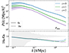 |
Fig. 1. DEMNUni-Cov power spectrum. Top: The solid and dashed lines represents the mean DEMNUni-Cov power spectrum, for three snapshots and the two cosmologies 0ν and 16ν. The corresponding shaded regions show the dispersion over the 50 realisations. The black short dashed line is the shot-noise level for the 10243 CDM particles. Bottom: Ratio between the mean power spectrum of the massive neutrino cosmology and the mass-less one. The grey area represents the dispersion over the 50 realisations at z = 0. |
2.2. The DEMNUni-Cov covariance matrix
All statistical quantities with a hat refer to estimators. We estimate the covariance matrix C of the power spectrum at a given redshift from the unbiased estimator
![Mathematical equation: $$ \begin{aligned} \hat{C}_{ij} = \frac{1}{N_{m-1}}\sum _{n = 1}^{N_m} \left[\hat{P}^{(n)}(k_i) - \bar{P}(k_i)\right]\left[\hat{P}^{(n)}(k_j) - \bar{P}(k_j)\right], \end{aligned} $$](/articles/aa/full_html/2025/01/aa47164-23/aa47164-23-eq1.gif) (1)
(1)
where  is the estimated power spectrum in the n-th realisation and
  is the estimated mean value of the power spectrum over the Nm realisations
 (2)
(2)
Assuming that the distribution of the power spectrum estimator is Gaussian, the covariance matrix estimator of Eq. (1) follows a Wishart distribution. Thus, one can express the variance of each individual elements of the estimated covariance matrix as (Wishart 1928)
![Mathematical equation: $$ \begin{aligned} V[{\hat{C}}_{ij}] = \dfrac{{\hat{C}}_{ij}^2 + {\hat{C}}_{ii}{\hat{C}}_{jj}}{N_m-1}. \end{aligned} $$](/articles/aa/full_html/2025/01/aa47164-23/aa47164-23-eq5.gif) (3)
(3)
On the other hand, one can formally express the covariance matrix of the power spectrum estimator as (Scoccimarro et al. 1999)
 (4)
(4)
where Mki is the number of independent modes in each Fourier shell centred on mode ki,  is the Kronecker symbol and
  is the shell-averaged trispectrum T defined by
 (5)
(5)
where the sum is made over two shells centred around ki and kj, and Vki, Vkj represent their respective Fourier volumes. Note that Eq. (4) is valid in the case of a periodic box, but in the presence of a survey window function the super sample covariance (SSC) term is also present (Takada & Hu 2013). From the simple structure of Eq. (4) one can split it into a Gaussian contribution CG(ki) (the diagonal term) and a non-Gaussian one  .
.
In Figure 2 we show, for the two extreme redshifts (0 and 2), the diagonal of the estimated covariance matrix in the massive neutrino cosmology, referred to as  (where the ‘D’ stands for DEMNUni). In addition, we represent the Gaussian contribution computed from the mean power spectrum
  . In the lower panel, we can see the variance excess carried by the trispectrum with respect to the Gaussian contribution, for k ≥ 0.2 h/Mpc and k ≥ 0.9 h/Mpc at z = 0 and z = 2 respectively. This reflects the non-linear evolution of the density field at these scales, which generates non-Gaussian higher-order correlation functions.
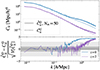 |
Fig. 2. Variance of the DEMNUni-Cov power spectrum. Top: Diagonal of the power spectrum covariance matrix in the 16ν cosmology, at z = 0 (blue) and z = 2 (purple). Solid lines show the variance estimated from the 50 DEMNUni-Cov realisations and the dashed lines display the Gaussian predictions. Bottom: Residuals between the estimated variance and the corresponding Gaussian prediction normalised by the error on the estimated covariance, given by Eq. (3). The grey areas represent the 1-σ and 3-σ levels of the residual. |
Figure 3 exhibits the correlation coefficients  between the different modes of the power spectrum. Those correlations would intrinsically be null for the off-diagonal elements in the Gaussian case. Similarly to what we saw on the diagonal elements, the non-Gaussian contributions appear at lower k at z = 0 than at z = 2. Indeed, at z = 2 and for k < 0.4 h/Mpc, the estimated correlations coefficients are compatible with zero, while significant positive correlations (ρij ∼ 0.6) are present at z = 0 for k > 0.3 h/Mpc.
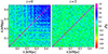 |
Fig. 3. Estimated power spectrum correlation matrix ρij from DEMNUni-Cov, at z = 0 (left) and z = 2 (right). |
Furthermore, these two figures show a large amount of noise in the estimated covariance matrix at all scales due to the low number of available simulations. From Eq. (3), the relative error of the diagonal elements is roughly 20%. Part of the present work aims at illustrating the propagation of the noise induced by the estimation of the covariance matrix elements into the cosmological parameter inference.
2.3. Sampling noise in the precision matrix
The statistical quantity involved in parameter estimation is actually the precision matrix Ψ ≡ C−1. An obvious estimator for Ψ would be the inverse of the estimated covariance matrix,  . As previously stated, the covariance matrix of Gaussian distributed data follows a Wishart distribution, so that its inverse follows an inverse Wishart distribution (Wishart 1928). It is therefore possible to compute the expectation value of the precision matrix estimator
  , which yields
 (6)
(6)
where Nb is the size of the data vector. This is showing that taking the inverse of the estimated covariance matrix in order to estimate the prediction matrix is introducing a predictable bias. It follows that an unbiased estimator of the precision matrix reads
 (7)
(7)
Since it was first introduced in a cosmological context by Hartlap et al. (2007), this correcting factor in Eq. (7) is often called the Hartlap factor.
We see from Eq. (6) that the bias constrains the precision matrix to be estimated with at least Nm > Nb + 2 and that, even with this condition satisfied, if Nm comparable to Nb this leads to a large bias. Because it is larger than 1, it means that due to a low sample size, the precision matrix is overestimated, i.e. the covariance is effectively underestimated. The main consequence for parameter inference is then an underestimation of the uncertainty on the determination of cosmological parameters.
Even with an unbiased precision matrix estimator, a small number of realisations leads to a noisy estimate of Ψ. We shall consider that the estimated precision matrix  can be decomposed in its true value Ψ and the error (or noise) on the truth ΔΨ, such that
  . Since ΔΨ originates from the propagation of a finite number of samples (realisations) of the measurement (here the power spectrum estimator) into the estimator of the precision matrix, we will refer to it as sampling noise. In the case where the estimated data-vector follows a Gaussian distribution, the covariance between the elements of the precision matrix
  is given as (Taylor et al. 2013)
 (8)
(8)
where
 (9)
(9)
Based on Eq. (8) and using the Fisher formalism, several authors have studied how random noise in the estimated precision matrix affects the estimation of cosmological parameters, in the case of Gaussian posteriors (Taylor et al. 2013; Dodelson & Schneider 2013; Percival et al. 2014; Taylor & Joachimi 2014). They found that it adds random noise both to the shape and the position of the posterior’s maximum. In the following we review the various effects that have to be taken into account in order to take the sampling noise into account in a cosmological parameter inference.
Let us denote the true error that would be obtained without sampling noise (i.e perfectly knowing the precision matrix) on a parameter θ as σθ, its estimation (from an estimated covariance matrix) as  and the corresponding best-fit value as
  . The impact of a noisy precision matrix on parameter inference can be summarised in three distinct effects.
(i) There is an additional variance on the variance of the estimated parameters (Taylor et al. 2013)
![Mathematical equation: $$ \begin{aligned} \mathrm{Var} [\hat{\sigma }^2_\theta ] = \dfrac{2}{N_m - N_b - 4}\sigma _\theta ^{4}. \end{aligned} $$](/articles/aa/full_html/2025/01/aa47164-23/aa47164-23-eq25.gif) (10)
(10)
(ii) There is also an additional variance on the position of the best-fit (Dodelson & Schneider 2013)
![Mathematical equation: $$ \begin{aligned} \mathrm{Var} [\hat{\theta }] = B(N_b - N_p)\sigma ^2_\theta , \end{aligned} $$](/articles/aa/full_html/2025/01/aa47164-23/aa47164-23-eq26.gif) (11)
(11)
where Np is the number of parameters to estimate. Note that the direction of this shift in the best-fit is completely stochastic.
(iii) The variance of a parameter estimated from the width of the posterior is biased (Percival et al. 2014)
![Mathematical equation: $$ \begin{aligned} \langle \hat{\sigma }^2_\theta \rangle = \left[ 1+A+B(N_p+1) \right] \sigma ^2_\theta . \end{aligned} $$](/articles/aa/full_html/2025/01/aa47164-23/aa47164-23-eq27.gif) (12)
(12)
This third effect should not be confused with the first one. The effect (i) is randomly modifying the size of the errors while (iii) is biasing their average size.
To account for these last two effects (ii) and (iii), Percival et al. (2014) proposed a corrective factor
 (13)
(13)
which should directly multiply  when quoting error-bars. In a critical case where A and B are non negligible ( Nm ∼ Nb), the numerator dominates for Nb ≫ Np, while the denominator dominates for Nb ∼ Np. In most cases, for cosmological analyses, the number of varied parameters is smaller than the number of data points. It means that the main effect coming from sampling noise is the stochastic shift of the posterior’s maximum, i.e. Eq. (11).
Presenting the estimated parameter uncertainty, without multiplying by  would not be representative of the actual error on
  . However, as discussed in Wadekar et al. (2020), blindly inflating parameter’s error-bars by
  has caveats that should be kept in mind. First, if one is interested not only in the confidence regions of the estimated parameters but also in its best-fit values, m1 does not correct for the stochastic shift of Eq. (11). Indeed, it only inflates the error-bars so that, on average, the best-fit lies in it. Finally, the predictions for these additional variance and bias, are only derived for Gaussian distributed parameters and data.
In Sect. 2.5, we will verify the effect of corrections (i), (ii) and (iii) individually. To this aim in the following we show how we design a reference realistic covariance matrix.
2.4. Fast Monte-Carlo catalogues with COVMOS
The COVMOS5 (Baratta et al. 2020, 2023) public code allows the fast realisation of catalogues of various cosmological tracers and models in real and redshift-space. Its fastness stems from the fact that no dynamical evolution is required, as it is usually done in an N-body simulation. Instead, a density field is directly generated at a given redshift, before being submitted to a local Poisson sampling to generate the point-like catalogue.
Although this kind of approach is widely studied in literature through the so-called Log-Normal mock generators (i.e. Xavier et al. 2016; Agrawal et al. 2017), the originality of COVMOS is that the power spectrum of the density and velocity fields, as well as the 1-point probability distribution function (PDF) of the density contrast δ, can be arbitrarily set by the user. Thus, it is not limited to the Log-Normal form of the PDF and enables more realistic models to be targeted.
Since generating a large number of realisations is easily achievable one can estimate a precision matrix with a negligible amount of noise. A possible application of this method is the production of the reference covariance matrix of the power spectrum estimator. It has been shown in Baratta et al. (2023) that the produced covariance, when compared with those estimated from N-body realisations, are faithfully reproduced in a certain range of scales. In real-space, mode correlations are reliably reproduced up to k = 0.3h/Mpc for z ≥ 0.5, while at z = 0, the certainty interval does not exceed k ≥ 0.17h/Mpc. Beyond this limit, correlations start to be progressively over-estimated.
In the present work we created two different COVMOS data sets:
-
The COVMOS_halofit data set which targets the 1-point density PDF estimated from the DEMNUni-Cov simulations and the Halofit power spectrum corresponding to the DEMNUni-Cov cosmology. We generated more than 100 000 of these catalogues for the 5 redshifts corresponding to the DEMNUni-Covsnapshots. We use this data set to study the NERCOME estimator in Sect. 2.5, sampling noise effect in Sect. 4.2 and non-Gaussian covariance in Sect. 5.
-
The COVMOS_demnuni data set which targets the 1-point density PDF and the power spectrum estimated from the DEMNUni-Cov simulations. This set is more realistic in terms of clustering as it reproduces the power spectrum from the N-body simulations. We generated 10 000 of these catalogues for the 5 redshifts. The same kind of setting was used in Baratta et al. (2023) to validate COVMOS against the DEMNUni-Cov simulations at level of the power spectrum and its covariance matrix. We used this data set to study the accuracy of the COVMOS covariance matrix at the level of parameter constraints in Sect. 4.3.
Both sets are characterised by negligible shot-noise compared to the measurements (np = 108 particles per realisation). They have been generated on periodic comoving volumes of size L = 1000 Mpc/h, with the COVMOS sampling parameter Ns = 512 (corresponding to the spatial resolution of 2 Mpc/h). The entire sample of simulation and associated power spectra estimation took ∼5 days, running on about 940 processors of 2.4 GHz of the Dark Energy Centre in Marseille, France. For a recap, Table 1 presents all the data sets that are used throughout the article and their characteristics.
Characteristics of the data sets used in this work; they are available at the five redshifts z = 0, 0.5, 1, 1.5, and 2.
2.5. Non-linear shrinkage with NERCOME
The NERCOME (Non-parametric Eigenvalue Regularised Covariance Matrix Estimator) algorithm was first proposed by Lam (2016) and then applied in a cosmological context by Joachimi (2017). This estimator is designed to reduce the bias and the variance present in an estimated precision matrix, which propagates to parameter estimation.
The NERCOME algorithm can be decomposed in 3 steps. Let us consider a set of Nm realisations of the data vector X of size Nb, from which we want to estimate the covariance:
-
Divide the set of realisations in two subsets of size s and Nm − s respectively.
-
Apply the standard covariance estimator to each subset to obtain the covariance matrices
 , with i = 1 or 2. Decompose them in the form
  , with U the matrix of eigenvectors and D the diagonal matrix of eigenvalues.
 -
Estimate the covariance matrix as
 (14)
(14)and average
 over Nc different random compositions of the subsets and a fixed split-position s.
In the original version of the algorithm the operation is repeated for different s to find the optimal split, but here, following Joachimi (2017), we will keep a fixed s = (2/3)Nm and Nc = 500.
An insight to understand Eq. (14), is that taking the diagonal of  , which mixes two matrices estimated from independent data sets, will shrink both large and small eigenvalues to avoid singular values6, so that
  is always positive definite.
Following Joachimi (2017), we can test the efficiency of NERCOME in reducing the bias and the variance in the estimated precision matrix, by considering the signal-to-noise ratio (S/N), defined as
 (15)
(15)
If it is estimated using a Hartlap-biased precision matrix, then the expectation value yields ![Mathematical equation: $ \langle \hat{ F} \rangle = \left[(N_m-1)/(N_m-N_b-2)\right] F $](/articles/aa/full_html/2025/01/aa47164-23/aa47164-23-eq40.gif) . So it is possible to measure the bias in
. So it is possible to measure the bias in  , by performing an average of the SNR over a certain number of realisations of the precision matrix, and to divide by the SNR computed with the true precision matrix, such that
 (16)
(16)
In the same way, one can show that
 (17)
(17)
is equivalent to the dispersion of the estimated precision matrix (Taylor & Joachimi 2014).
In practice, we can check Eqs. (16) and (17) using the COVMOS_demnuni catalogues (see Table 1). Indeed we can divide the 10 000 realisations into at least 10 groups of 1000 realisations. This way we can estimate 10 times the precision matrix  for both the standard estimator and NERCOME using Nm realisations among the 1000 remaining ones. We can finally estimate the left hand side of Eqs. (16) and (17). As data-vector we use the estimated power spectrum in Nb = 40 k-shells.
In the upper panel of Figure 4 we see that the prediction is in agreement with the expected bias from the Hartlap correction. In addition, as expected, the bias diverges when Nm is approaching Nb + 2. Instead, even when Nm < Nb + 2, NERCOME is able to produce a non-singular covariance matrix at the expense of introducing a bias.
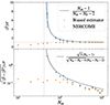 |
Fig. 4. Bias (top) and dispersion (bottom) of the S/N defined in Eq. (15) when the precision matrix is estimated from Nm realisations and a data vector of size Nb = 40. The blue and orange filled circles respectively correspond to the biased (i.e. without the Hartlap correction) and NERCOME estimator. The black line represents the predictions from Eqs. (16) (top) and (17) (bottom). The vertical dashed grey line indicates the Hartlap limit Nm ≤ Nb + 2. |
In the lower panel of Figure 4, despite the fact that we estimate the dispersion only on 10 realisations, we observe that the trend followed by the obvious estimator of the precision matrix is matching the expected one. Finally, NERCOME is significantly reducing the dispersion. These results are in agreement with Joachimi (2017). We will test the reliability of a covariance matrix estimated with NERCOME at the level of parameter estimation in Sect. 4.2.
3. Parameter inference
In this section we present the methodology we follow to assess how noise in the estimator of the precision matrix propagates to the Bayesian inference of cosmological parameters.
3.1. Likelihood
We assume the estimator of the power spectrum  follows a Nb-variate Gaussian distribution, thus the Likelihood function
  takes the following form
![Mathematical equation: $$ \begin{aligned} -2\log {L} = [\hat{\boldsymbol{P}}(k) - \boldsymbol{P}(k; \boldsymbol{\theta })]^T \mathbf C ^{-1} [\hat{\boldsymbol{P}}(k) - \boldsymbol{P}(k; \boldsymbol{\theta })] \equiv \chi ^2, \end{aligned} $$](/articles/aa/full_html/2025/01/aa47164-23/aa47164-23-eq47.gif) (18)
(18)
where  is the data vector of dimension Nb, θ is the set of free cosmological parameters, P(k; θ) is the theoretical prediction depending on the cosmological parameters, and C is the covariance matrix. The non-linear theoretical prediction for the CDM+baryon is obtained from CLASS (Blas et al. 2011, version 2.9) with the Halofit (Smith et al. 2003) prescription incorporating the treatment of massive neutrinos by Bird et al. (2012) and the revised fitting formulae of Takahashi et al. (2012).
In order to maximise the statistical power of the Likelihood we combine the five redshifts at our disposal in a single parameter inference. Note that despite being unrealistic we use the z = 0 power spectrum because it includes a higher level of non-linear clustering which results in more mode coupling through the off-diagonal of the covariance matrix. This is a very interesting case that happens at z = 0 in ΛCDM but which could happen at higher redshift in different cosmological models or simply when adding a survey window function.
The data vector is taken from five independent realisations at the corresponding redshifts. This is allowing to consider them as being independent. Thus, the combined log-Likelihood function can be expressed as the sum of the log-Likelihood of each redshift
 (19)
(19)
Note that the effective size of the data vector remains Nb at a single redshift.
We vary the reduced baryon and CDM densities ωb and ωcdm7, the normalised expansion rate parameter h ≡ H0/100 and the single neutrino mass mν8. The priors on these parameters are chosen to be broad and uniform to avoid further effects on parameter inference output. They are listed in Table 2 along with their true (fiducial) values. We also consider the case of a tighter Gaussian prior coming from Big Bang Nucleosynthesis (BBN) for ωb in Sect. 5. The public code MontePython (Brinckmann & Lesgourgues 2019, version 3.3.0) is running the Monte Carlo Markov Chains allowing to explore the parameter space. We use GetDist (Lewis 2019) to produce the plots of the posterior distribution of the inferred cosmological parameters. The convergence of the chains is asserted with a Gelman-Rubin criterion (Gelman & Rubin 1992) : R − 1 < 0.01.
Uniform priors for cosmological parameters and fiducial values for the 16ν cosmology.
3.2. Observable space
In common clustering analysis based on spectroscopic catalogues of galaxies, one has to infer comoving distances from redshifts. Thus, we should know the cosmological parameters before analysing the data. That is the reason why a cosmology has to be guessed to go from the redshift to the comoving distance. However, this is introducing the Alcock-Paczyński distortion which has to be taken into account in a parameter inference based on the statistical properties of the galaxy density. In practice, the expansion rate parameter H0 generates a completely isotropic distortion which can be easily taken into account by simply expressing all comoving distances in Mpc/h. As a result it is current to convert all comoving distances in simulations to mimic the fact we know the comoving distance up to some factor of h. However, this is introducing a degeneracy in the parameter space (see Appendix A for more details). In Sect. 4 we are interested in the effect of sampling noise on the parameters posterior distribution, thus we need to control the shape of the posterior and in particular control whether it presents or not non-Gaussian features. Hence for that section we chose to perform our fits using measurements of the power spectrum in comoving units of Mpc−1. Instead, in Sect. 5 we include the isotropic re-scaling by h of the comoving distances in the simulation, this is allowing to get more realistic shape for the parameter posterior distribution.
4. Sampling noise effects on cosmological parameter estimation
In this section we start by showing the effect of sampling noise on the estimated covariance matrix using the DEMNUni-Cov data. Then, we assess the performances of NERCOME based on the 100 000 COVMOS_halofit realisations in order to finally compare the covariance matrix of DEMNUni-Cov estimated with NERCOME to the covariance matrix estimated from COVMOS.
4.1. Parameter inference with a high sampling noise
We focus on showing the propagation of the noise in the estimation of the covariance matrix to the Bayesian inference on cosmological parameters. To this aim, we use a data vector made of the power spectrum estimated in the 16ν cosmology of the DEMNUni-Cov simulations following the setting described in Sect. 3. We allow the size Nb of the data vector to vary according to the maximum wave number kmax kept in the likelihood analysis.
We take the Gaussian covariance matrix CG, described in Sect. 2.2, as a reference. This way, we compare the cosmological inference obtained from the raw precision matrix (inverse of  ) estimated from Nm = 45 DEMNUni-Cov realisations, together with the Hartlap corrected one and finally we add the m1 correction to the posterior parameter distribution. In the case of the Gaussian covariance we limit the kmax to avoid taking a too high level of non-linear coupling. Thus, based on Figure 2, we will allow kmax to vary on the range [0.1, 0.275] h/Mpc, which corresponds to varying the data vector size Nb from 16 to 44. Regarding the DEMNUni-Cov estimated covariance matrix (
 ) we are constrained to have Nb < Nm − 2 in order to be able to correct from the Hartlap factor and avoid having a singular matrix. We thus, require that Nb ≤ 39 which corresponds to kmax varying on the range [0.1, 0.25] h/Mpc.
Figure 5 shows the 2D posteriors obtained for kmax = 0.2 h/Mpc with the Gaussian covariance and the DEMNUni-Cov covariance, corrected or not for the Hartlap bias, as well as the posterior distribution inflated by the m1 factor. We can see that considering the Gaussian covariance CG all input parameters are retrieved within the 68% level. Instead, a clear shift of the posterior is observed when considering the estimated DEMNUni-Cov covariance matrix. As expected, that shift is the same for the three other cases: raw, Hartlap corrected and m1 corrected. This is because the Hartlap correction multiplies all the elements of the covariance matrix and the m1 correction directly affects the posterior. Since the data vector is the same in the four considered cases, the observed shift is only due to the choice of the covariance matrix. The theoretical ground for this shift was presented in the work of Sellentin (2020) in the context of blinding strategies for data analysis. It actually shows that a constant re-scaling of the precision matrix will not change the posterior position.
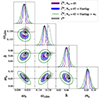 |
Fig. 5. 2D and 1D marginalised posteriors, obtained for kmax = 0.19 h/Mpc, with the analytic Gaussian covariance (grey), the covariance estimated from 45 DEMNUni-Cov spectra without the Hartlap correction (purple), with the Hartlap correction (blue), and with the m1 factor (green). For the 2D posteriors, the 68.3% and 95.5% confidence regions are shown. The black square and dashed lines show the fiducial (true) cosmology. |
Comparing the width of the posteriors we can observe different effects that were explained in Sect. 2.3. Without the Hartlap correction on  , the posterior width is underestimated, in comparison with CG. When correcting for the Hartlap bias, one can observe that the width of the posterior is increasing to reach a similar size as in the Gaussian case. By further inflating the errors by
  , we can gauge the effect of the noise in
  , transferred to the cosmological parameters, which is not accounted for by the Hartlap factor. This huge error-bar accounts for the stochastic shift in the position of the best-fit that was discussed above.
To further gauge the effect of sampling noise in the precision matrix, we show in Figure 6 the marginalised parameter constraints for the four previously considered cases as well as their corresponding reduced chi-square χ2/nd.o.f. (where nd.o.f. = Nb − Np is the number of degrees freedom) with respect to the chosen maximum wave mode kmax.
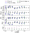 |
Fig. 6. Marginalised parameter constraints, derived from the same cases as in Figure 5. The four top panels represent the relative difference with the 16ν cosmology for each free parameter. The bottom panel shows the χ2 over nd.o.f.. On this last panel the green and blue dots overlap because the difference is just in the presence of m1 which does not affect the χ2. |
As the Gaussian covariance is noise-free, the fluctuations in the constraints that we see while varying kmax are only due to the noise present in the data vector. Hence, it can serve as a reference to exhibit the noise in the estimated covariance. Overall, for all considered kmax < 0.25 h/Mpc the estimated cosmological parameters with the Gaussian covariance are in agreement at the 99% level with the true cosmological parameters.
Looking at the constraints obtained with the DEMNUni-Cov covariance, we observe larger fluctuations through the kmax range, showing the effect of sampling noise. Focusing on the error bars, we can see the same effects that were discussed above with the Hartlap and m1 factor. Here we can appreciate how the intensity of these effects grow with kmax as the corresponding size Nb of the data vector increases. Indeed, for all parameters, taking into account both the Hartlap factor and the m1 correction allows to recover the true value of cosmological parameters at the 99% level.
The χ2/nd.o.f. is stable and remains close to 1 in the case of the Gaussian covariance, indicating a good-fit. However, it is overestimated by a factor of 2 (or more for large kmax) in the case of the DEMNUni-Cov covariance without the Hartlap correction. Conversely, when accounting for the Hartlap bias, the χ2 is lower than 1. This result was explained by Sellentin & Heavens (2016a) who showed that the  estimated with a Hartlap-biased precision matrix is drawn from a distribution with a larger width than a true χ2 distribution. On the contrary when it is corrected for the Hartlap bias, the distribution is sharper.
Finally in Figure 7, we expose the FoM computed from the above constraints, following the same colour code as in the two previous figures. Again, we clearly see the overestimation of the FoM when the Hartlap bias is not accounted for. For kmax < 0.15 h/Mpc, the Hartlap factor seems sufficient to recover the FoM obtained with the Gaussian covariance, which can be considered as a reference at these scales. But, as we can see in Figure 6, the best-fit values present large deviations on those scales especially for h and mν. This is illustrated by the decrease of the FoM caused by the m1 factor, which accounts for this fluctuation in the best fit. Furthermore, note that with both corrections, the FoM decreases as the kmax is getting close to the limit Nb = Nm − 2. In that case the Hartlap bias and sampling noise are so high that increasing the amount of information in the fit by increasing the kmax degrades the constraints. This is exactly what we have to avoid.
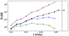 |
Fig. 7. FoM obtained from the parameter constraints in the 16ν cosmology for the same cases and with the same colour code as in Figures 5 and 6. The vertical dashed line shows the kmax corresponding to the limit Nb = Nm − 2, above which the covariance matrix estimated with Nm = 45 cannot be inverted. |
We have explicitly shown the effect of the Hartlap bias on parameter inference, and how the sampling noise present in the precision matrix can drastically impact the constraints on cosmological parameters. In the next sections we will show how NERCOME and COVMOS can mitigate these two effects.
4.2. Reduction of sampling noise with NERCOME
The aim of this section is to test whether NERCOME can reduce the effect of sampling noise in the precision matrix, while resulting in unbiased cosmological constraints. To isolate the effects coming from sampling noise, it is better if the parameter inference is not affected by biases due to the modelling of the non-linear power spectrum, or to the fact that the covariance matrix is not perfectly describing the data. To overcome these issues, in this section, we chose to use the COVMOS_halofit data set both for the data vector and the covariance matrix. In this way we make sure we have the exact modelling and covariance for our data.
4.2.1. Performance at low Nm
A way to estimate the dispersion of the best-fit and error of cosmological parameters due to sampling noise, is to run several fits on the same data vector for different realisations of the precision matrix. From the 100 000 COVMOS_halofit power spectra we can create 100 different subsets, each containing Nm = 45 realisations. The precision matrix is estimated on each of these subsets, with the Hartlap-corrected estimator (Eq. (7), dubbed standard estimator in the following) and NERCOME.
We perform 100 MCMC’s at a fixed kmax = 0.2 h/Mpc (corresponding to data vector size Nb = 30), with the two different estimators for the precision matrix:
-
Standard estimator, with Nm = 45, referred to as S45,
-
NERCOME with Nm = 45, referred to as N45.
We have access to the distribution of best-fits and errors for the four cosmological parameters obtained from the two precision matrices (S45 and N45). As a reference, we also perform a fit with the covariance matrix estimated with Nm = 100 000, which can be considered as the true covariance. This is done in the 16ν cosmology so that mν is well constrained and we only deal with Gaussian posterior distributions (c.f. Figure 5).
In Figure 8, we examine the distribution of the best-fit for S45 and N45, compared to the best-fit obtained using the true covariance. Table 3 gathers the useful statistics characterising these distributions for each parameter. First we can see that the true values of the cosmological parameters are recovered within, or very close to the 68% level (indicate on the plot with a grey shaded area) in the case of the true covariance matrix. Regarding S45 and N45, the dispersion of the best-fit is about the same order of magnitude as the true error σθ (see Table 3) for each considered cosmological parameters. However, NERCOME reduces the dispersion from around 130 to 70% of the true error, which corresponds to a decrease between ∼35 and 50% depending on the parameter (see Table 3).
Best fit dispersion and its reduction with NERCOME. The two rows on the top present the dispersion of the best fit relative to the error estimated with the true covariance and the last row presents the reduction of the best-fit variance thanks to NERCOME.
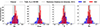 |
Fig. 8. Distribution of the estimated best fit on cosmological parameters ωb, ωcdm, h, and mν (from left to right) obtained for each of the 100 evaluations of the covariance matrix (Nm = 45) when considering the standard estimator S45 (blue histogram) or NERCOMEN45 (orange histogram). The black vertical line shows the best fit estimated with the true covariance matrix and its associated error represented by grey shaded area. The dotted vertical line referred to as fiducial in the inset displays the true cosmology. The dashed line represents a Gaussian centred on the true best fit which dispersion is given by the prediction of Dodelson & Schneider (2013) (c.f. Eq. (11)). |
Looking at Figure 8 we can see that for both S45 and N45, the average deviation of the best-fit with respect to the truth is not statistically significant, no matter what is the considered cosmological parameter. This means that if the data vector is giving a parameter constraint which is within the 68% level, then the propagation of noise from the estimated precision matrix cannot introduce a significant bias in the analysis. Although, NERCOME is less affected by the noise, if the data vector points to a cosmology which is at around 95% confidence level, then noise in the covariance could lead to a biased estimation (more than 99% level) of the parameters. Finally, we can see that the prediction from Dodelson & Schneider (2013) (Eq. (11)) is in good agreement with the distributions for S45 shown in Figure 8. This means that one could take it into account in the same way as the m1 correction, by inflating artificially the errors on the estimated parameters.
After analysing the effect of sampling noise on the best-fit, let us focus on the uncertainty on each parameter. Figure 9 shows the distribution of the variance,  (σ2(θ) in the abscissa label) for S45 and N45, compared to the variance σθ2 estimated using the true covariance. In the S45 case, the dispersion of the parameter variances correspond to about 25% of the true variance for all cosmological parameters. While in the case of N45, we estimate that NERCOME reduces the variance on the variance by 30% for all parameters except for the baryonic density ωb.
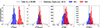 |
Fig. 9. Distribution of the estimated variance on cosmological parameters ωb, ωcdm, h, and mν (from left to right) obtained for each of the 100 evaluations of the covariance matrix (Nm = 45) when considering the standard estimator S45 (blue histogram) or NERCOMEN45 (orange histogram). The vertical black line shows the variance estimated with the true covariance matrix. The dashed black curve represents a Gaussian distribution centred on the true variance (solid black line) and which dispersion is given by Taylor et al. (2013) (c.f. Eq. (10)), that is, the reason why it extends to negative values which is of course mathematically impossible. |
In addition, NERCOME exhibits a systematic overestimation of the parameter variance. Indeed, when using a covariance matrix estimated with NERCOME, the cosmological parameters variances are overestimated by about 17% for ωcdm, 30% for h and mν and by a factor of 2 for ωb. Instead, when considering the S45 estimator we cannot detect a significant bias in the estimation of parameter uncertainties.
Finally, in Figure 9 we show a Gaussian distribution with a dispersion corresponding to the prediction of Taylor et al. (2013) (Eq. 10) and centred on the true value of the estimated variance. One can conclude that the predicted dispersion is overestimated, thus the represented Gaussian extends to negative values for the estimated variance. This is clearly mathematically impossible and is only due to our choice of representing a Gaussian when the true distribution is certainly not Gaussian, but we stress that this does not change the conclusion.
4.2.2. Evolution with Nm
In this section, we study the dependence of the results obtained in the previous section with respect to the number of realisations Nm used to estimate the covariance. As a result, we will focus on the following statistics: ![Mathematical equation: $ \mathrm{Var}[\hat\theta] $](/articles/aa/full_html/2025/01/aa47164-23/aa47164-23-eq59.gif) giving the variance of the estimated best-fit,
giving the variance of the estimated best-fit, ![Mathematical equation: $ \mathrm{Var}[\hat\sigma_\theta^2] $](/articles/aa/full_html/2025/01/aa47164-23/aa47164-23-eq60.gif) which is the variance of the estimated parameter variance and
which is the variance of the estimated parameter variance and  assessing the bias in the estimation of the parameter variance.
With the 100 000 COVMOS_halofit realisations we create 100 subsets of up to Nm = 1000 realisations. This way for each subset we can estimate the precision matrix. We keep kmax = 0.2 h/Mpc corresponding to Nb = 30 as in the previous sub-section.
In the case of the standard estimator, the dispersion on the best-fit (left panel of Figure 10) is following the analytical prediction by Dodelson & Schneider (2013). In addition, we clearly see the effect of NERCOME which reduces this dispersion when the number of realisations Nm used to estimate the precision matrix is low. We also see that the variance of the best-fit obtained with NERCOME converges quickly (Nm ∼ 100) towards the one expected with the standard estimator. In addition, when Nm > 100 the variance of the best fit is lower than half the variance on the fitted parameters.
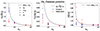 |
Fig. 10. Effects of sampling noise propagating the parameter constraints (best fit and variance). The results are shown for the 16ν cosmology, resulting in a Gaussian posterior distribution. Left: ratio of the variance on the best-fit to the true variance of the parameters, compared to black line showing the prediction of Dodelson & Schneider (2013) (Eq. (11)). Middle: ratio of the variance of the estimated variance of the parameters to the true square of the parameter variance, compared to the solid line showing the prediction of Taylor et al. (2013)(Eq. (10)). Right: ratio of the mean estimated variance of the parameters to the true variance of the parameter compared to solid line showing the prediction of Percival et al. (2014)(Eq. (12)). |
The middle panel of Figure 10 focuses on the variance of the estimated parameter variance. It is showing that NERCOME only marginally reduces it compared to the standard estimator. One can also see that even when Nm is increasing the dispersion of the variance of the fitted parameters is systematically lower (roughly a factor of 2) than expected by Taylor et al. (2013). Anyway, this contribution drops around 1% for Nm = 100 which makes it the least dominant contribution to the total error budget.
Finally, the left panel of Figure 10 is representing the bias in the estimation of the variance of the cosmological parameters, which appears to be surprisingly negligible. Indeed, it is much smaller than the one expected from Eq. (12). Instead, we can notice that NERCOME is introducing a significant systematic overestimation of the variance of the cosmological parameters.
While we find the predictions from Taylor et al. (2013) and Percival et al. (2014) to disagree with our estimations, it is important to note that they correspond to small effects and that at least they appear to be conservative. In the end, this shows that for what concerns the error on cosmological parameters it seems equivalent to use the standard covariance estimator and to inflate error-bars by  or to use NERCOME. Indeed, the bias on the variance of parameters we get when using NERCOME is about the same order as the best-fit dispersion we get when using the standard estimator (which is what
  corrects for).
In conclusion, although NERCOME is quite efficient in reducing the dispersion on the best-fit in a low Nm regime, the resulting estimated errors on parameters are biased high. Thus, NERCOME might be used to gauge by how much the constraints one gets from an analysis are affected by the dispersion of the best-fit and to get a more precise idea of the best-fit position, but we cannot fully trust the resulting error bars.
4.2.3. Non-Gaussian posterior
One final test we want to conduct is to study the impact of a non-Gaussian posterior distribution on the performance of NERCOME and on sampling noise effects in general. To do so we perform the same analysis as in the previous section but in the 0ν cosmology. In this case, since the true value of the neutrino mass is mν = 0, the estimated posterior distribution is cut by the physical prior mν > 0 (c.f. Appendix B for an example). In consequence the main assumption of the analytic predictions is broken. In that case, as in the Gaussian posterior case, we take the diagonal of the parameter covariance matrix, estimated from the MCMC, to be the variance of cosmological parameters to which we compare the analytical predictions.
Figure 11 presents the same result as Figure 10 but for the 0ν cosmology. For the dispersion on the best-fit and the bias on the variance (left and right panels) we observe the same behaviour as in the case of Gaussian posteriors. However, the variance on the estimated variance (middle panel) is now larger than the expected one when considering the neutrino mass mν. Moreover, in that case NERCOME is quite efficient in mitigating this effect as it reduces the variance on the variance of mν by a factor 2 for Nm = 45. Despite this increase of the dispersion of the variance one should apply the same procedure as in the Gaussian case in order to be more conservative.
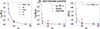 |
Fig. 11. Same as Figure 10, but for the 0ν cosmology, resulting in a non-Gaussian posterior distribution. |
As a last comment, from both Figures 10 and 11, we remark a certain scattering between the cosmological parameters. It might come from the different correlations among the parameters making them react in different ways to covariance effects. Still, we find the same order of magnitude from one parameter to another.
4.3. Reliability of COVMOS for parameter inference
Thanks to the efficiency of COVMOS to produce a high number of realisations, the effect of sampling noise in the precision matrix can be reduced to a negligible amount. However, it is not guaranteed that the method results in an accurate covariance matrix. Indeed, it was shown in Baratta et al. (2023) that at z = 0, COVMOS over-predicts non-diagonal elements of the real space covariance for k > 0.17h/Mpc. It is therefore important to asses whether these deviations, in the COVMOS covariance with respect to the accurate (but noisy) DEMNUni-Cov covariance, bias the estimation of cosmological parameters. If we see no bias we also want to insure that the uncertainties on cosmological parameters are not over- or under-estimated when using a COVMOS covariance.
If we compare the results obtained from a COVMOS covariance with the one obtained from a DEMNUni-Cov covariance estimated with the standard estimator, it will be hard to draw conclusions given the large influence of sampling noise in the latter case due to the low number of realisations (c.f. Sect. 4.1), especially on the best-fit. Thus, we also include the DEMNUni-Cov covariance estimated with NERCOME, as it was shown to result in reduced best-fit dispersion in the previous section. This will also allow one to compare in a common setting the result of the two approaches, NERCOME and COVMOS, at the level of the parameters best-fit position. However, it was observed in Sect. 4.2 that NERCOME leads to bias in the estimated variance of parameters. Hence we will not be able to make a rigorous comparison at the level of parameters error-bar.
We use the DEMNUni-Cov power spectra as our data vector (still at the 5 redshifts). We make this choice because we want to test the capability of COVMOS to provide an unbiased parameter estimation in a realistic case. Here we mean realistic in the way that COVMOS should be used, i.e. cloning an existing data-set to enlarge its number of realisations. In other words, we test, at the level of the estimated parameters, how well COVMOS can reproduce the DEMNUni-Cov simulations9.
In order to account for the intrinsic noise in the data vector, we fit three different data sets, Data1, Data2 and Data3. Each of them, containing one independent realisation of the power spectrum per redshift, taken from the 50 DEMNUni-Cov. Note that we performed the same analysis for 10 possible independent combinations of data, but we only show three of them for clarity because it does not change the conclusions.
For the covariance matrix, as explained above we consider three cases:
-
 , standard. A covariance matrix estimated with the standard estimator from the Nm = 45 remaining DEMNUni-Cov realisations. We correct for the Hartlap bias in the precision matrix but we don’t apply the m1 factor to the resulting constraints.
 -
 , NERCOME. Same as above but with NERCOME.
 -
 , a covariance matrix estimated from the Nm = 10 000 COVMOS_demnuni realisations (c.f. Sect. 2.4).
Finally, in order to focus on the effect of the covariance, we consider only kmax < 0.2 h/Mpc to limit the impact of potential biases coming from the modelling of the non-linear power spectrum (c.f. 4.1).
Figure 12 displays individual parameter constraints with respect to the their true values obtained from the 1D marginalised posteriors of cosmological parameters as well as the corresponding χ2/nd.o.f. with respect to kmax. We summarise the relevant information based on Figure 12 in the following:
-
Some points feature asymmetric error-bars, indicating that the posteriors are not Gaussian, especially at low k. This is mostly due to the fact that, in some cases the estimation of mν is compatible with 0, forcing the posterior to be cut at the low boundary of the prior on this parameter.
-
At kmax = 0.1 h/Mpc, for all parameters, and covariances, the scatter on the best-fit, for the different data-sets is larger than for higher kmax. This comes from the intrinsic variance of the power spectrum which is larger on large scales and is also reflected in the parameter error-bars which, are larger for this scale cut.
-
On the left panel, corresponding to the standard DEMNUni-Cov covariance, we can see a large scatter of the best-fit across the kmax range. The same applies for the χ2. This indicates that with such covariance, we can potentially have an estimation of cosmological parameters which greatly deviates from the truth, by more than 3σ in some cases. It was expected and already observed in Sect. 4.1.
-
In contrast, by looking at the middle panel, the DEMNUni-Cov covariance estimated with NERCOME, exhibits more stable constraints with respect to kmax, thanks to the diminution of the best-fit scattering observed in the previous section. However, in some cases we see a systematic deviation from the fiducial cosmology, larger than 1σ. This is present especially in the case of Data2, which does not agree with the two others, especially for h. This disagreement mainly comes from residual sampling noise in this covariance matrix.
-
Finally, on the right panel, when the parameters are estimated, using the COVMOS covariance matrix, the best-fits are generally more centred on the fiducial values. This can be seen especially in the case of Data2. Considering all the data-sets, the COVMOS covariance gives a close to 1σ agreement for all parameters in the kmax range [0.15, 0.2] h/Mpc. In addition, the χ2/nd.o.f. is stable and close to 1 for all data-sets.
For completeness we also show in Figure 13 the 2D marginalised posteriors, only in the (ωcdm, mν) plane for simplicity, for all data-sets and covariances. We clearly see the advantage of using COVMOS here, as in the two other cases the estimated parameter posteriors present a bias (at more than 95%) with respect to the true cosmology. In addition, we see again that with NERCOME although the ellipses are less scattered than with the standard estimator  , their width are overestimated compared to the two other cases.
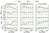 |
Fig. 12. Parameter constraint with respect to kmax, for three different sets of DEMNUni-Cov realisations: DEMNUni-Cov01-05 in blue, DEMNUni-Cov06-10 in orange, and DEMNUni-Cov46-50 in green. The three columns correspond to the covariance matrix which was used in the fits: standard DEMNUni-Cov covariance with Nm = 45 and corrected for the Hartlap bias (left), NERCOMEDEMNUni-Cov covariance with Nm = 45 (middle) and standard COVMOS covariance with Nm = 10 000 (right). The top rows show the relative difference with respect to the fiducial cosmology for each parameter and the bottom row the χ2/nd.o.f.. |
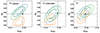 |
Fig. 13. 2D marginalised posteriors in the (ωcdm, mν) plane, for kmax = 0.19 h/Mpc. The colours correspond to the three different data sets as in Figure 12. The three panels correspond to the considered covariances. The black dashed lines and the square show the fiducial cosmology. |
We now focus on parameter’s uncertainties to check whether these are not over- or under-estimated. The metric we consider for this is the Figure of Merit (FoM), defined as
 (20)
(20)
where  is the estimated parameter covariance matrix. It is inversely proportional to the hyper-volume delimited by the 2σ contours in the full parameter space. The higher is the FoM, the tighter are the constraints. In Figure 14, we present the FoM with respect to kmax, for all the considered cases:
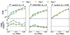 |
Fig. 14. FoM with respect to kmax. The top panel shows the FoM for the three different DEMNUni-Cov. The bottom panel shows the ratio of the FoM obtained with the standard (left) and NERCOME (middle) estimation of the DEMNUni-Cov covariance, to the FoM obtained with COVMOS (right). |
-
As expected, the FoM increases with kmax, because the number of available modes in the power spectrum increases.
-
Similarly to the best-fit, the FoM is scattered along the kmax range in the case of the standard DEMNUni-Cov covariance. This dispersion is lessen for the two other covariances.
-
In the case of the standard and NERCOME estimation of
 the FoM also presents a dispersion among the three data vectors, which is less important for COVMOS. This is a combined effect of both changing the data and the covariance for the first two cases10, while the COVMOS covariance is fixed.
 -
Despite this dispersion, the standard DEMNUni-Cov covariance generally results in a higher FoM than in the case of COVMOS, while NERCOME gives a slightly lower FoM for kmax > 0.15 h/Mpc, which confirms what was observed above.
As noted before, it is hard to draw rigorous conclusions on whether the constraints we obtain with COVMOS present accurate errors because we are comparing it with constraints affected by sampling noise effects. However, we saw in Sect. 2.5 that (i) sampling noise affects marginally the estimated error-bars and (ii) NERCOME tends to result in overestimated error-bars. Thus, given the above observation that the FoM obtained with COVMOS is slightly smaller (by a factor ∼0.5 on average) than the one obtained with the standard  and close to the one obtained with the NERCOME
 , it seems that COVMOS leads to slightly overestimated error-bars.
Still, inferring such conclusions only on the basis of a FoM comparison can be a bit misleading as this metric also includes correlation between parameters. While, the above argument is based on the results of Sect. 2.5 where we were only considering the error-bars. In addition, by visually comparing the size of the ellipses of the right and left panels in Figure 13, the difference between the standard  and the COVMOS case is not that obvious. A more thorough study is required to confirm the above observation and is left for future work.
Finally, we can conclude that, thanks to COVMOS it is possible to completely erase the effects of sampling noise, at the cost of a negligible computing time compared to N-body simulations. We have shown that when using a COVMOS covariance matrix for parameter inference the constraints present no bias on the best-fit but possibly a slight overestimation of errors. It also appears to be the method offering the most stable results. Thus, in the next section we will use the COVMOS covariances.
5. Impact of the non-Gaussian part of the covariance on cosmological constraints
In this section we study how the non-Gaussian part of the power spectrum covariance is affecting constraints on cosmological parameters. In particular we quantify the bias on the best-fit values and on their estimated error when neglecting the non-Gaussian contribution to the power spectrum covariance (i.e. CiNG in Eq. (4)).
5.1. Methodology
We consider three cases for describing the power spectrum covariance:
-
The theoretical Gaussian covariance (i.e. CG in Eq. (4)) computed with the fiducial Halofit power spectrum;
-
A covariance matrix estimated from the COVMOS realisations, but setting to zero all the off-diagonal elements, thus accounting only for the diagonal part of CiNG;
-
The full COVMOS covariance matrix with all diagonal and non-diagonal elements.
This way it is possible to asses which part of the covariance has the greatest influence on cosmological constraints. To this aim, We perform the fit of the power spectrum in the 16ν cosmology and consider a similar procedure as described in Sect. 2, with few modifications.
First, we choose to perform the parameter inference in the h/Mpc space, thus accounting for the isotropic AP effect (c.f. Sect. 3.2 and Appendix A) to assess the effect of CiNG with more realistic parameter degeneracy. Second, we choose the data-vector to be one realisation (per redshift) of the COVMOS_halofit data-set. This is allowing to remove any uncertainty in the modelling and focus on the effect of the choice of the covariance. Thus, it follows that the reference covariance matrix is the one estimated with Nm = 100 000 COVMOS_halofit realisations.
Finally, as mentioned above, the parameter space is expected to be more degenerate when including the isotropic AP. Thus, in addition to the uninformative uniform priors described in Table 2 we also consider a Gaussian prior on the baryonic density ωb. Its central value is chosen to be the true value in the DEMNUni cosmology and its width is set by Big Bang Nucleosynthesis (BBN) results (Cooke et al. 2018):
 (21)
(21)
As shown in Figure 15 this prior allows to break a strong degeneracy between ωb and mν (among other parameters). In addition, it confirms that the true cosmology is well recovered within the 68% contour level. This is the case for all parameters and for all the scale cuts considered kmax ∈ [0.1, 0.3] h/Mpc as shown in Appendix C. The constraints discussed in this example are obtained using the full reference COVMOS covariance.
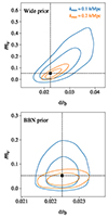 |
Fig. 15. 2D marginalised posteriors in the (ωb, mν) plane, for kmax = 0.1 and 0.2 h/Mpc. The 2 panels correspond to the type of prior considered on ωb. The black dashed lines and the square show the fiducial cosmology. |
5.2. Effect on the estimation of parameter’s errors
We first quantify the impact of CiNG on cosmological parameters errors, to this aim we define the ratio
 (22)
(22)
where σθG and σθiNG are respectively the errors on the cosmological parameter θ obtained using as covariance CG and CG + CiNG (i.e. the COVMOS covariance).
In Figure 16 we show R(θ) for the whole kmax range, with or without the BBN prior and accounting or not for the off-diagonal elements of CiNG. Without the latter and when the BBN prior is applied on ωb, the ratio is close to one for all parameters no matte how is chosen kmax. In particular, for ωb, the prior is so restrictive that the error is not affected at all by the choice of the covariance. By releasing this prior the parameter uncertainty increases by 5 to 10% depending on the parameter. Hence, the diagonal part of CiNG does not seem to have a large impact on cosmological constraints even for kmax 0.3 h/Mpc. We recall that at these scales the total power spectrum variance is larger than the Gaussian one by about 2-σ, as seen in Figure 2 with the DEMNUni-Cov covariance. In addition this is a conservative result as the COVMOS covariance we are considering here is slightly overestimating the DEMNUni-Cov one for k > 0.17 h/Mpc as reported in Baratta et al. (2023).
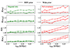 |
Fig. 16. Ratio R between the parameter uncertainties obtained with the non-Gaussian covariance CiNG and the Gaussian one CG. In the left panel we only consider the contribution to the diagonal and in the left panel off-diagonal terms are also accounted for. The dashed and plain lines correspond respectively to the uniform and Gaussian BBN priors on ωb. |
When adding the off-diagonal terms R(θ) increases significantly for all parameters, except for ωb when it is restricted to the BBN prior, where it is still unaffected by the choice of the covariance. As expected R(θ) increases with kmax because the correlations between the Fourier modes come from non-linear clustering which is more important when probing small scales. In addition, this increase in R(θ) starts at kmax = 0.15 h/Mpc, which reflects the scale below which clustering is still linear and thus the non-Gaussian contribution to the covariance is negligible.
It is of great interest to notice that the most affected parameter is the neutrino mass mν. Indeed, even when the BBN prior is applied, the ratio R(mν) grows linearly from 1 to 1.4 between kmax = 0.15 to 0.3 h/Mpc. In contrast, for h and ωcdm, the ratio reaches a maximum of 1.25 and 1.2 respectively. Without the BBN prior, R(ωb) is at most ∼1.2 and all the other parameters take a +0.1 on R(θ) at all kmax. This reflects how a prior on ωb can affect the other parameters through their correlations. In the rest of the analysis we always apply the BBN prior on ωb.
Note that mν is the parameter which uncertainty is the most affected by the choice of the covariance matrix. This is counter intuitive because we would naively expect that the most affected parameters would be those to which the power spectrum are more sensitive like ωc or h. A possible explanation for that could be the large degeneracy of the neutrino mass with both the matter density and the normalised Hubble parameter or the fact that the neutrino mass is close to zero.
5.3. Best-fit position of parameters
We have seen in the previous section that CiNG and in particular its off-diagonal elements affect significantly the error on cosmological parameters. Because we perform this analysis in a MCMC framework we also have the possibility to check whether the position of the best-fit is affected.
Figure 17 exhibits the 1D and 2D marginalised posterior distributions for kmax = 0.25 h/Mpc in the three covariance cases. As expected from the previous section, the diagonal non-Gaussian contribution has almost no effect on the constraints and the posteriors obtained in that case and with the Gaussian covariance are similar and well centred on the fiducial cosmology. However when adding the off-diagonal terms the posterior drifts away from the fiducial cosmology in particular for h and mν with a shift of the order of 1σ. Note that here the most shifted parameters are h and mν, which we remind to be the most and the least constrained parameters respectively.
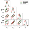 |
Fig. 17. 2D and 1D marginalised posteriors, obtained with the Gaussian covariance (black), the diagonal (green), and full (red) non-Gaussian covariance from COVMOS, for kmax = 0.25 h/Mpc. The black square and dashed lines show the fiducial cosmology. |
To asses whether this shift of the best-fit is systematic or stochastic we perform the same fit but for 50 different realisations of the data-vector taken from the COVMOS_halofit data-set. In Figure 18 we show the distribution of the best-fits obtained from these 50 fits using either the Gaussian or full non-Gaussian covariance, as well as the residual between the two distributions normalised by the quadratic sum of the errors obtained in each of the fits. This latter quantity is also known as the pull and defined as
 (23)
(23)
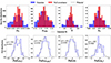 |
Fig. 18. Results from fitting 50 different realisations of the COVMOS_halofitP(k) at kmax = 0.25 h/Mpc. Top: Normalised distribution of best-fits in the case of the Gaussian (blue) and full covariance (red). Bottom: Normalised distribution of the pull as defined in Eq. (23). The black dashed line is a Gaussian fit to the histogram. The mean and standard deviation obtained from the fit for each parameter are written in each panel. |
it tells how significant is the change in the best-fit position.
First, looking at the distribution of the best-fits we can see that on average the fiducial cosmology is well retrieved for the two covariances. In addition, the distribution of the pull is close to a Gaussian distribution with a mean equal to 0, meaning that the shift of the best-fit is purely stochastic. Performing a Gaussian fit of this distribution we indeed find the fitted mean to be compatible with zero for all parameters. This also gives us the standard deviation of the pull distribution which can indicates which are the most affected parameters by this stochastic shift and by how much in terms of the fraction of their error bars. As observed in the lower panel of Figure 18, h and mν are the parameters with the higher standard-deviation of the Pull statistic, σ = 0.8 and 0.6 respectively. This indicates that for those two parameters the distribution of the best-fit is not significantly different when considering the Gaussian or the full covariance matrix. We also did the same study for kmax = 0.2 h/Mpc and found the same effect but with lower dispersion. For that kmax the standard deviations found from fitting a Gaussian to the pull distribution are at maximum σ = 0.5 and 0.4, for h and mν respectively.
Sellentin & Starck (2019) demonstrated that assuming an incorrect covariance matrix could bias parameter inference. Here we showed that this bias exists but does not have a preferred direction over multiple realisations of the data vector. In practice, we have a single realisation of a measured cosmological observable, those results are showing that data should not be analysed with a single choice for describing the covariance matrix. Indeed, it is important to gauge how the data react to a change in the covariance matrix in order to draw similar conclusions on the parameter inference.
Finally, from the top panel of Figure 18 we can see that the full covariance allows to get a smaller dispersion of the best-fit compared to the one obtained when considering the Gaussian one. This appears to be counter intuitive because the 95% contour identified by the 2D-posterior obtained from the full covariance is wider than the Gaussian one. Therefore, we would have expected that varying the data, the best-fit would have followed the same trend. A possible explanation is to consider that the Gaussian covariance does not offer an accurate enough description of the measurements. Indeed this is demonstrated in Appendix B of Payerne et al. (2023), where they show that, for a Gaussian likelihood, the ensemble covariance matrix of the estimated parameters (i.e. obtained from an ensemble of estimated best-fit values) and the individual one (i.e. obtained from the width of an individual posterior) are different if the assumed data covariance matrix deviates from the true one. More precisely, if the true data covariance matrix is larger than the assumed one then the ensemble variance of parameters is larger than the individual one. This directly applies in our case by identifying the Gaussian covariance matrix to the assumed one and the COVMOS covariance matrix to be the true one.
5.4. Discussion
We have seen that the posterior distribution of cosmological parameters is significantly affected by the off-diagonal elements of the covariance matrix. The width of the posterior is underestimated for kmax > 0.15 h/Mpc when assuming a Gaussian (diagonal) covariance. In addition, for kmax > 0.2 h/Mpc, the best-fit values experiences a stochastic shift that can reach 1-σ if an incorrect covariance is assumed. It is difficult to understand why some parameters are more affected than others as, in our analysis, the most affected ones are both the most and the least constrained (h and mν respectively). In addition, we note that the presence of a tight prior, on ωb, strongly reduces this effect.
We remind readers that the analysis setup chosen in this work is quite far from what is actually accessible with galaxy clustering surveys because we are considering here the matter field in real space. However, this is what weak lensing surveys are probing through the statistics of the distortions of the shape of galaxies. Although here we are considering 3D P(k) instead of projected quantities along the line of sight as it is the case for weak lensing and we are not sensitive at all to the systematics characteristic of weak lensing analysis, these results on the matter field can be of direct interest to interpret parameter inference with weak lensing. In addition, our results are consistent with Barreira et al. (2018b) who showed that the in survey non-Gaussian contribution to the covariance (dubbed cNG in their paper, for ‘connected non-Gaussian’) has a non negligible impact on cosmological constraints obtained with weak lensing, though the SSC contribution seems to be the most important one.
Note that Wadekar et al. (2020) also tested the impact of non-Gaussian contributions to the covariance using an analytical covariance accounting for non-linear galaxy bias and RSD in the case of the full-shape galaxy clustering spectroscopic analysis of BOSS DR12 data. They found non-Gaussian covariance effects to be negligible on cosmological parameters because they are absorbed by nuisance parameters (mainly galaxy bias) through marginalisation. This was also observed in Gouyou Beauchamps et al. (2021) for SSC in the case of photometric galaxy clustering. In another work, Yu et al. (2023) used the same data as in Wadekar et al. (2020) but a hybrid approach for the covariance matrix, combining analytical prediction and simulations to show that the non-Gaussian covariance could be responsible for a 10-20% increase in cosmological parameters errors11. It is thus unclear how important these additional terms to the covariance are. It would be interesting to pursue these studies that have been done with BOSS data, for stage-IV galaxy survey settings as they should be more sensitive to non-Gaussian covariance by probing smaller and more non-linear scales than stage-III surveys such as BOSS. The present work, which is a first step before adding complexity to the analysis, will certainly be useful to interpret future results.
Finally, we only considered our data to be in periodic boxes. In the more realistic case of a survey window function other terms to the covariance should be considered, not only SSC terms which are non-Gaussian. Indeed, due to the mode mixing introduced by the survey window function, the Gaussian covariance becomes non-diagonal (Li et al. 2019). This is left for future work.
Given the exploratory nature of our work and the simplifications we chose to make, especially not considering RSD, galaxy bias and survey footprint, we can try to anticipate how our results would change in presence of such realistic effects. (i) The parameter space to be marginalised over would be much larger due to the addition of nuisance parameters needed to model the aforementioned effects, such as galaxy bias or parameters modelling galaxies velocity for RSD. Thus, the relative impact of non-Gaussian covariance would be diluted in the uncertainty increase due to the enlarged parameter space. This was observed for example in Euclid Collaboration (2024). (ii) It was shown in Baratta et al. (2023) that RSD tend to decrease the amplitude of the trispectrum, so the importance of the non-Gaussian covariance term of the covariance would also be reduced in this case. (iii) As said above the presence of a survey window function gives rise to additional Gaussian covariance that mixes the Fourier modes. The presence of these non-diagonal terms could also dilute the Fourier mode mixing due to non-linear clustering. Overall, in a more realistic scenario, we can expect a weaker impact of the non-Gaussian term of the covariance. This aspect still needs to be investigated in more detail in future works.
6. Conclusions
In order to be able to get a precise measurement of the still undetected total neutrino mass from the LSS of the Universe, upcoming galaxy surveys will need to probe small scales where the matter field presents non-Gaussian features that appear in the covariance of its power spectrum in the form of the trispectrum. In this article we show that, to be sure we accurately and precisely detect subtle effects on the LSS such as massive neutrino free streaming, we need an almost perfect understanding of the covariance of the observable.
There are two complementary ways to model the covariance matrix: through analytical computation, which generally requires the use of perturbative expansions, or by directly estimating it from simulations, which must be numerous enough for the estimate not to be too noisy. In this work we focus on the latter path and explain, in Sect. 4, two techniques used to reduce the influence of covariance sampling noise in parameter inference.
We first considered NERCOME, a non-linear shrinkage covariance estimator. We find this estimator to significantly reduce the dispersion of the best-fit parameters but at the cost of a systematic increase in the estimated errors on the parameters. Thus, while NERCOME can be useful to get a more accurate position of the best fit when only a low number of simulations is available for estimating the covariance matrix, the estimated error bars are overestimated.
We also tested how well the Fisher-forecast-based analytical prescription performed at predicting sampling noise effects. While the formula from Dodelson & Schneider (2013) is in good agreement with the observed dispersion of the best-fit values of parameters, we find the prediction of the variance on the variance and the bias on the variance by Taylor et al. (2013) and Percival et al. (2014) to overestimate them. In addition, those contributions are subdominant with respect to the dispersion of the best fit. At the same time, we verified that a non-Gaussian posterior distribution does not affect the above conclusions.
The second technique we considered to deal with a low number of simulations to estimate the covariance is COVMOS. We find the best-fit values of cosmological parameters estimated using a COVMOS covariance matrix to be unbiased, thus demonstrating the potential of this method for the analysis of future galaxy surveys. However, we could not precisely evaluate how accurate parameters’ error bars are when using COVMOS. This is something that should be quantitatively evaluated in a future work.
Then, in Sect. 5 we focused on the impact of the in-survey non-Gaussian term of the power spectrum covariance, CiNG (c.f. Eq. (4)), coming from the LSS non-linear evolution, on cosmological parameters’ posterior distribution. We show that the diagonal part of CiNG does not affect cosmological constraints but it is rather the correlation between the different modes (i.e. the off-diagonal part) that produces an effect. When considering this non-Gaussian covariance, the error bars on cosmological parameters increase significantly for kmax > 0.15 h/Mpc, when compared to the Gaussian covariance case. In particular, the error increase for h and mν goes up to 20% and 30%, respectively, for kmax = 0.25 h/Mpc. This happens when we restrict ωb with a BBN prior; otherwise, the increase is even higher (30% and 40%, respectively).
Furthermore, we see that CiNG could also affect the position of the best fit for kmax > 0.2 h/Mpc. By performing MCMCs on multiple realisations of the data, we do indeed find that when assuming the incorrect covariance, the best-fit values of parameters undergo a stochastic shift with respect to the value obtained with the true covariance. At kmax = 0.25 h/Mpc and for the most affected parameters, h and mν, this shift is of the same order as their statistical errors. It is thus important to account for non-Gaussian covariance not only to get the true errors on cosmological parameters but also to get an accurate estimate of their central value.
As we considered the matter power spectrum in real space in a periodic box, the non-Gaussian term CiNG here refers to the trispectrum contribution correlating Fourier modes inside the observed volume (c.f. Eq. (5)). Thus, SSC as well as contribution from a survey window function in the Gaussian term was not accounted for. Also, shot-noise-related terms (Lacasa 2018) were neglected as we were working with a negligible shot-noise level.
The covariance matrix is a complex and rich statistical object and its accurate prediction is one of the most important challenges that upcoming galaxy surveys will have to face. There are many different possible approaches (analytical, semi-analytical, N-body simulations, approximated simulations, etc.) to model a variety of terms arising from non-linear clustering, galaxy bias, shot noise, survey window function, observational systematics, and more. It is therefore mandatory for the data analysis of future surveys, such as Euclid, DESI, or LSST, to know which terms are dominant and must be accounted for. To understand the hierarchy of covariance terms, it is interesting to tackle the problem step by step, by adding complexity as we go further. This is what the present work aims and it should certainly be pursued in the future.
These are methods designed to estimate the covariance matrix directly from the data.
These are the reduced baryon and CDM densities ωb and ωcdm (where ωi ≡ Ωih2), the Hubble constant h ≡ H0/100, and the neutrino mass mν. More details on the parameter space is given in Sect. 3.
Of course, if one considers galaxies in redshift space, one must add nuisance parameters and power spectrum multipoles in the likelihood, thus increasing Np and Nb. But this only changes the overall amplitude of sampling noise effects.
This shrinkage is said to be non-linear because it shrinks different eigenvalues by different amounts. See Pope & Szapudi (2008) for a reference on linear shrinkage.
Where ωi ≡ Ωih2.
As stated in Sect. 2.1 the 16ν cosmology assumes a degenerate mass eigenstate, so that it makes no difference to fit for Mν or mν.
The validation has been made at the level of the power spectrum, the 2-pt correlation function and their covariance matrices in Baratta et al. (2023).
For a selection of 5 DEMNUni-Cov realisations going to the data vector, the covariance is estimated on the remaining 45 simulations. So, when the data vector is changed, the covariance also changes.
Apart from the different treatment of the covariance, the other main methodological difference between Yu et al. (2023) and Wadekar et al. (2020) is that in the former work they performed a template fit (i.e. fixing the shape of the power spectrum and fitting for the AP parameters and the velocity growth factor fσ8) while in the latter it was a full-shape fit.
Acknowledgments
The authors would like to thank Constantin Payerne and Calum Murray for useful discussions. PB and SGB were supported by CNES, focused on Euclid mission. This work received support from the French government under the France 2030 investment plan, as part of the Excellence Initiative of Aix-Marseille University -A*MIDEX (AMX-19-IET-008 -IPhU). The DEMNUni simulations were carried out in the framework of “The Dark Energy and Massive-Neutrino Universe” project, using the Tier-0 IBM BG/Q Fermi machine and the Tier-0 Intel OmniPath Cluster Marconi-A1 of the Centro Interuniversitario del Nord-Est per il Calcolo Elettronico (CINECA). We acknowledge a generous CPU and storage allocation by the Italian Super-Computing Resource Allocation (ISCRA) as well as from the coordination of the “Accordo Quadro MoU per lo svolgimento di attività congiunta di ricerca Nuove frontiere in Astrofisica: HPC e Data Exploration di nuova generazione”, together with storage from INFN-CNAF and INAF-IA2.
References
- Agrawal, A., Makiya, R., Chiang, C.-T., et al. 2017, JCAP, 10, 003 [CrossRef] [Google Scholar]
- Avila, S., Murray, S. G., Knebe, A., et al. 2015, MNRAS, 450, 1856 [NASA ADS] [CrossRef] [Google Scholar]
- Baratta, P., Bel, J., Plaszczynski, S., & Ealet, A. 2020, A&A, 633, A26 [NASA ADS] [CrossRef] [EDP Sciences] [Google Scholar]
- Baratta, P., Bel, J., Gouyou Beauchamps, S., & Carbone, C. 2023, A&A, 673, A1 [NASA ADS] [CrossRef] [EDP Sciences] [Google Scholar]
- Barreira, A., Krause, E., & Schmidt, F. 2018a, JCAP, 10, 053 [CrossRef] [Google Scholar]
- Barreira, A., Krause, E., & Schmidt, F. 2018b, JCAP, 2018, 015 [Google Scholar]
- Bayer, A. E., Villaescusa-Navarro, F., Massara, E., et al. 2021, ApJ, 919, 24 [NASA ADS] [CrossRef] [Google Scholar]
- Bernardeau, F., Colombi, S., Gaztanaga, E., & Scoccimarro, R. 2001, Phys. Rep., 367, 1 [Google Scholar]
- Bird, S., Viel, M., & Haehnelt, M. G. 2012, MNRAS, 420, 2551 [Google Scholar]
- Blas, D., Lesgourgues, J., & Tram, T. 2011, JCAP, 2011, 034 [Google Scholar]
- Blot, L., et al. 2019, MNRAS, 485, 2806 [NASA ADS] [CrossRef] [Google Scholar]
- Brinckmann, T., & Lesgourgues, J. 2019, Phys. Dark Univ., 24, 100260 [Google Scholar]
- Carbone, C., Petkova, M., & Dolag, K. 2016, JCAP, 2016, 034 [CrossRef] [Google Scholar]
- Cooke, R., Pettini, M., & Steidel, C. C. 2018, ApJ, 855, 102 [NASA ADS] [CrossRef] [Google Scholar]
- DESI Collaboration (Aghamousa, A., et al.) 2016, arXiv e-prints [arXiv:1611.00036] [Google Scholar]
- Dodelson, S., & Schneider, M. D. 2013, Phys. Rev. D, 88, 063537 [Google Scholar]
- Escoffier, S., Cousinou, M. C., Tilquin, A., et al. 2016, arXiv e-prints [arXiv:1606.00233] [Google Scholar]
- Euclid Collaboration (Sciotti, D., et al.) 2024, A&A, 691, A318 [NASA ADS] [CrossRef] [EDP Sciences] [Google Scholar]
- Friedrich, O., Seitz, S., Eifler, T. F., & Gruen, D. 2016, MNRAS, 456, 2662 [NASA ADS] [CrossRef] [Google Scholar]
- Fumagalli, A., Biagetti, M., Saro, A., et al. 2022, JCAP, 12, 022 [Google Scholar]
- Gelman, A., & Rubin, D. B. 1992, Stat. Sci., 7, 457 [Google Scholar]
- Gouyou Beauchamps, S., Lacasa, F., Tutusaus, I., et al. 2021, A&A, 659, A128 [Google Scholar]
- Hand, N., Feng, Y., Beutler, F., et al. 2018, AJ, 156, 160 [Google Scholar]
- Hartlap, J., Simon, P., & Schneider, P. 2007, A&A, 464, 399 [NASA ADS] [CrossRef] [EDP Sciences] [Google Scholar]
- Heavens, A., Sellentin, E., de Mijolla, D., & Vianello, A. 2017, MNRAS, 472, 4244 [NASA ADS] [CrossRef] [Google Scholar]
- Hu, W., & Kravtsov, A. V. 2002, ApJ, 584, 702 [Google Scholar]
- Izard, A., Crocce, M., & Fosalba, P. 2015, MNRAS, 459, 2327 [Google Scholar]
- Joachimi, B. 2017, MNRAS, 466, L83 [NASA ADS] [CrossRef] [Google Scholar]
- Kitaura, F.-S., Yepes, G., & Prada, F. 2014, MNRAS, 439, 21 [Google Scholar]
- Lacasa, F. 2018, A&A, 615, A1 [NASA ADS] [CrossRef] [EDP Sciences] [Google Scholar]
- Lacasa, F. 2020, A&A, 634, A74 [NASA ADS] [CrossRef] [EDP Sciences] [Google Scholar]
- Lam, C. 2016, Ann. Stat., 44, 928 [Google Scholar]
- Laureijs, R., Amiaux, J., Arduini, S., et al. 2011, arXiv e-prints [arXiv:1110.3193] [Google Scholar]
- Lesgourgues, J., & Pastor, S. 2006, Phys. Rept., 429, 307 [NASA ADS] [CrossRef] [Google Scholar]
- Lewis, A. 2019, arXiv e-prints [arXiv:1910.13970] [Google Scholar]
- Li, Y., Schmittfull, M., & Seljak, U. 2018, JCAP, 2018, 022 [CrossRef] [Google Scholar]
- Li, Y., Singh, S., Yu, B., Feng, Y., & Seljak, U. 2019, JCAP, 01, 016 [NASA ADS] [Google Scholar]
- LSST Science Collaboration (Abell, P. A., et al.) 2009, arXiv e-prints [arXiv:0912.0201] [Google Scholar]
- Mohammad, F. G., & Percival, W. J. 2022, MNRAS, 514, 1289 [NASA ADS] [CrossRef] [Google Scholar]
- Monaco, P., Theuns, T., & Taffoni, G. 2002, MNRAS, 331, 587 [Google Scholar]
- Parimbelli, G., Anselmi, S., Viel, M., et al. 2021, JCAP, 2021, 009 [Google Scholar]
- Parimbelli, G., Carbone, C., Bel, J., et al. 2022, JCAP, 2022, 041 [Google Scholar]
- Payerne, C., Murray, C., Combet, C., et al. 2023, MNRAS, 520, 6223 [NASA ADS] [CrossRef] [Google Scholar]
- Paz, D. J., & Sanchez, A. G. 2015, MNRAS, 454, 4326 [NASA ADS] [CrossRef] [Google Scholar]
- Percival, W. J., Ross, A. J., Sanchez, A. G., et al. 2014, MNRAS, 439, 2531 [NASA ADS] [CrossRef] [Google Scholar]
- Philcox, O. H. E., Ivanov, M. M., Zaldarriaga, M., Simonovic, M., & Schmittfull, M. 2021, Phys. Rev. D, 103, 043508 [NASA ADS] [CrossRef] [Google Scholar]
- Planck Collaboration XVI. 2014, A&A, 571, A16 [NASA ADS] [CrossRef] [EDP Sciences] [Google Scholar]
- Pope, A. C., & Szapudi, I. 2008, MNRAS, 389, 766 [NASA ADS] [CrossRef] [Google Scholar]
- Scoccimarro, R., Zaldarriaga, M., & Hui, L. 1999, ApJ, 527, 1 [NASA ADS] [CrossRef] [Google Scholar]
- Sefusatti, E., Crocce, M., Scoccimarro, R., & Couchman, H. 2016, MNRAS, 460, 3624 [NASA ADS] [CrossRef] [Google Scholar]
- Sellentin, E. 2020, MNRAS, 492, 3396 [Google Scholar]
- Sellentin, E., & Heavens, A. F. 2016a, MNRAS, 456, L132 [Google Scholar]
- Sellentin, E., & Heavens, A. F. 2016b, MNRAS, 464, 4658 [Google Scholar]
- Sellentin, E., & Starck, J.-L. 2019, JCAP, 08, 021 [Google Scholar]
- Smith, R. E., Peacock, J. A., Jenkins, A., et al. 2003, MNRAS, 341, 1311 [Google Scholar]
- Takada, M., & Hu, W. 2013, Phys. Rev. D, 87, 123504 [NASA ADS] [CrossRef] [Google Scholar]
- Takahashi, R., Sato, M., Nishimichi, T., Taruya, A., & Oguri, M. 2012, ApJ, 761, 152 [Google Scholar]
- Taylor, A., & Joachimi, B. 2014, MNRAS, 442, 2728 [Google Scholar]
- Taylor, P. L., & Markovič, K. 2022, Phys. Rev. D, 106, 063536 [NASA ADS] [CrossRef] [Google Scholar]
- Taylor, A., Joachimi, B., & Kitching, T. 2013, MNRAS, 432, 1928 [Google Scholar]
- Upham, R. E., Brown, M. L., & Whittaker, L. 2021, MNRAS, 503, 1999 [NASA ADS] [CrossRef] [Google Scholar]
- Viel, M., Haehnelt, M. G., & Springel, V. 2010, JCAP, 06, 015 [CrossRef] [Google Scholar]
- Wadekar, D., & Scoccimarro, R. 2020, Phys. Rev. D, 102, 123517 [NASA ADS] [CrossRef] [Google Scholar]
- Wadekar, D., Ivanov, M. M., & Scoccimarro, R. 2020, Phys. Rev. D, 102, 123521 [CrossRef] [Google Scholar]
- Wishart, J. 1928, Biometrika, 20A, 32 [CrossRef] [Google Scholar]
- Xavier, H. S., Abdalla, F. B., & Joachimi, B. 2016, MNRAS, 459, 3693 [NASA ADS] [CrossRef] [Google Scholar]
- Yu, B., Seljak, U., Li, Y., & Singh, S. 2023, JCAP, 2023, 057 [Google Scholar]
- Zennaro, M., Bel, J., Villaescusa-Navarro, F., et al. 2017, MNRAS, 466, 3244 [NASA ADS] [CrossRef] [Google Scholar]
Appendix A: Impact of the isotropic Alcock-Paczyński effect on parameter degeneracy
In this appendix we show with an example the difference between performing a fit of the full shape of the P(k) with h/Mpc or Mpc−1 units. As explained in section 3.2 this can be understood as accounting or not for the isotropic Alcock-Paczyński effect.
For this example we ran a MCMC fit of the P(k), at the 5 redshifts, of one realisation of the COVMOS_halofit data-set and used 100 000 realisations to estimate the covariance matrix. Note that we apply the scale cut in the h/Mpc space in all cases such that the number of k bins considered is the same and the scale ranges probed are equivalent in both observable spaces.
Figure A.1 shows the 2D and 1D marginalised posteriors obtained when performing the fit in h/Mpc or Mpc−1. We can see that releasing the dependence in h in the units of the P(k) and the k grid brings strong degeneracies between all fitted cosmological parameters. Due to this degeneracies the posterior distribution presents non-Gaussian features, especially for mν. Here the fit is done using a covariance matrix with negligible sampling noise. However, as we want to study what happens with a noisy covariance matrix, the posterior will surely move around the parameter space due to this noise and thus could present even stronger non-Gaussian features. To have a better control on the shape of the posterior we choose to perform the fits in the Mpc−1 space.
These strong degeneracies could be broken by applying more restrictive priors on some of the parameters, for example on ωb with a prior coming from BBN results. In section 4 we don’t want the results to be affected by prior effects, but we consider this option in section 5.
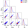 |
Fig. A.1. 2D and 1D marginalised posteriors, obtained performing the fit in the h/Mpc or Mpc−1 space. For the 2D posteriors, the 68.3% and 95.5% confidence regions are shown. This is the constraints for kmax = 0.19 h/Mpc. The black square and dashed lines show the fiducial 16ν cosmology. |
Appendix B: Non-Gaussian posterior
In this appendix we show how performing a fit in the 0ν cosmology results in non-Gaussian posteriors.
For this example we ran a MCMC fit of the P(k), at the 5 redshifts, of one realisation of the COVMOS_halofit data-set and used 100 000 realisations to estimate the covariance matrix, for each of the two cosmologies.
Figure B.1 shows the 2D and 1D marginalised posteriors we obtain. We can see that as mν = 0 in the 0ν cosmology, the MCMC is forced to sample the parameter space which is close to the physical prior mν > 0. Thus, the marginalised posterior of mν is highly non-Gaussian. Because of the correlation between mν and ωb the latter also exhibits a non-Gaussian marginalised posterior distribution.
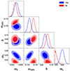 |
Fig. B.1. 2D and 1D marginalised posteriors, obtained in the 0ν or the 16ν cosmology. For the 2D posteriors, the 68.3% and 95.5% confidence regions are shown. This is the constraints for kmax = 0.2 h/Mpc. |
Appendix C: Effect of BBN prior on parameters contours
In this appendix we show the full triangle plots corresponding to Figure 15. Figures C.1 and C.2 exhibits the contours of all parameters for the wide and BBN prior cases respectively, for 3 different kmax covering the whole range of scale cuts we consider in this work.
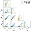 |
Fig. C.1. 2D and 1D marginalised posteriors, obtained in the 16ν cosmology with wide priors on all parameters, for 3 different scale cuts. For the 2D posteriors, the 68.3% and 95.5% confidence regions are shown. |
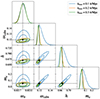 |
Fig. C.2. 2D and 1D marginalised posteriors, obtained in the 16ν cosmology with a BBN prior on ωb, for 3 different scale cuts. For the 2D posteriors, the 68.3% and 95.5% confidence regions are shown. |
All Tables
Characteristics of the data sets used in this work; they are available at the five redshifts z = 0, 0.5, 1, 1.5, and 2.
Uniform priors for cosmological parameters and fiducial values for the 16ν cosmology.
Best fit dispersion and its reduction with NERCOME. The two rows on the top present the dispersion of the best fit relative to the error estimated with the true covariance and the last row presents the reduction of the best-fit variance thanks to NERCOME.
All Figures
|
Fig. 1. DEMNUni-Cov power spectrum. Top: The solid and dashed lines represents the mean DEMNUni-Cov power spectrum, for three snapshots and the two cosmologies 0ν and 16ν. The corresponding shaded regions show the dispersion over the 50 realisations. The black short dashed line is the shot-noise level for the 10243 CDM particles. Bottom: Ratio between the mean power spectrum of the massive neutrino cosmology and the mass-less one. The grey area represents the dispersion over the 50 realisations at z = 0. |
| In the text | |
|
Fig. 2. Variance of the DEMNUni-Cov power spectrum. Top: Diagonal of the power spectrum covariance matrix in the 16ν cosmology, at z = 0 (blue) and z = 2 (purple). Solid lines show the variance estimated from the 50 DEMNUni-Cov realisations and the dashed lines display the Gaussian predictions. Bottom: Residuals between the estimated variance and the corresponding Gaussian prediction normalised by the error on the estimated covariance, given by Eq. (3). The grey areas represent the 1-σ and 3-σ levels of the residual. |
| In the text | |
|
Fig. 3. Estimated power spectrum correlation matrix ρij from DEMNUni-Cov, at z = 0 (left) and z = 2 (right). |
| In the text | |
|
Fig. 4. Bias (top) and dispersion (bottom) of the S/N defined in Eq. (15) when the precision matrix is estimated from Nm realisations and a data vector of size Nb = 40. The blue and orange filled circles respectively correspond to the biased (i.e. without the Hartlap correction) and NERCOME estimator. The black line represents the predictions from Eqs. (16) (top) and (17) (bottom). The vertical dashed grey line indicates the Hartlap limit Nm ≤ Nb + 2. |
| In the text | |
|
Fig. 5. 2D and 1D marginalised posteriors, obtained for kmax = 0.19 h/Mpc, with the analytic Gaussian covariance (grey), the covariance estimated from 45 DEMNUni-Cov spectra without the Hartlap correction (purple), with the Hartlap correction (blue), and with the m1 factor (green). For the 2D posteriors, the 68.3% and 95.5% confidence regions are shown. The black square and dashed lines show the fiducial (true) cosmology. |
| In the text | |
|
Fig. 6. Marginalised parameter constraints, derived from the same cases as in Figure 5. The four top panels represent the relative difference with the 16ν cosmology for each free parameter. The bottom panel shows the χ2 over nd.o.f.. On this last panel the green and blue dots overlap because the difference is just in the presence of m1 which does not affect the χ2. |
| In the text | |
|
Fig. 7. FoM obtained from the parameter constraints in the 16ν cosmology for the same cases and with the same colour code as in Figures 5 and 6. The vertical dashed line shows the kmax corresponding to the limit Nb = Nm − 2, above which the covariance matrix estimated with Nm = 45 cannot be inverted. |
| In the text | |
|
Fig. 8. Distribution of the estimated best fit on cosmological parameters ωb, ωcdm, h, and mν (from left to right) obtained for each of the 100 evaluations of the covariance matrix (Nm = 45) when considering the standard estimator S45 (blue histogram) or NERCOMEN45 (orange histogram). The black vertical line shows the best fit estimated with the true covariance matrix and its associated error represented by grey shaded area. The dotted vertical line referred to as fiducial in the inset displays the true cosmology. The dashed line represents a Gaussian centred on the true best fit which dispersion is given by the prediction of Dodelson & Schneider (2013) (c.f. Eq. (11)). |
| In the text | |
|
Fig. 9. Distribution of the estimated variance on cosmological parameters ωb, ωcdm, h, and mν (from left to right) obtained for each of the 100 evaluations of the covariance matrix (Nm = 45) when considering the standard estimator S45 (blue histogram) or NERCOMEN45 (orange histogram). The vertical black line shows the variance estimated with the true covariance matrix. The dashed black curve represents a Gaussian distribution centred on the true variance (solid black line) and which dispersion is given by Taylor et al. (2013) (c.f. Eq. (10)), that is, the reason why it extends to negative values which is of course mathematically impossible. |
| In the text | |
|
Fig. 10. Effects of sampling noise propagating the parameter constraints (best fit and variance). The results are shown for the 16ν cosmology, resulting in a Gaussian posterior distribution. Left: ratio of the variance on the best-fit to the true variance of the parameters, compared to black line showing the prediction of Dodelson & Schneider (2013) (Eq. (11)). Middle: ratio of the variance of the estimated variance of the parameters to the true square of the parameter variance, compared to the solid line showing the prediction of Taylor et al. (2013)(Eq. (10)). Right: ratio of the mean estimated variance of the parameters to the true variance of the parameter compared to solid line showing the prediction of Percival et al. (2014)(Eq. (12)). |
| In the text | |
|
Fig. 11. Same as Figure 10, but for the 0ν cosmology, resulting in a non-Gaussian posterior distribution. |
| In the text | |
|
Fig. 12. Parameter constraint with respect to kmax, for three different sets of DEMNUni-Cov realisations: DEMNUni-Cov01-05 in blue, DEMNUni-Cov06-10 in orange, and DEMNUni-Cov46-50 in green. The three columns correspond to the covariance matrix which was used in the fits: standard DEMNUni-Cov covariance with Nm = 45 and corrected for the Hartlap bias (left), NERCOMEDEMNUni-Cov covariance with Nm = 45 (middle) and standard COVMOS covariance with Nm = 10 000 (right). The top rows show the relative difference with respect to the fiducial cosmology for each parameter and the bottom row the χ2/nd.o.f.. |
| In the text | |
|
Fig. 13. 2D marginalised posteriors in the (ωcdm, mν) plane, for kmax = 0.19 h/Mpc. The colours correspond to the three different data sets as in Figure 12. The three panels correspond to the considered covariances. The black dashed lines and the square show the fiducial cosmology. |
| In the text | |
|
Fig. 14. FoM with respect to kmax. The top panel shows the FoM for the three different DEMNUni-Cov. The bottom panel shows the ratio of the FoM obtained with the standard (left) and NERCOME (middle) estimation of the DEMNUni-Cov covariance, to the FoM obtained with COVMOS (right). |
| In the text | |
|
Fig. 15. 2D marginalised posteriors in the (ωb, mν) plane, for kmax = 0.1 and 0.2 h/Mpc. The 2 panels correspond to the type of prior considered on ωb. The black dashed lines and the square show the fiducial cosmology. |
| In the text | |
|
Fig. 16. Ratio R between the parameter uncertainties obtained with the non-Gaussian covariance CiNG and the Gaussian one CG. In the left panel we only consider the contribution to the diagonal and in the left panel off-diagonal terms are also accounted for. The dashed and plain lines correspond respectively to the uniform and Gaussian BBN priors on ωb. |
| In the text | |
|
Fig. 17. 2D and 1D marginalised posteriors, obtained with the Gaussian covariance (black), the diagonal (green), and full (red) non-Gaussian covariance from COVMOS, for kmax = 0.25 h/Mpc. The black square and dashed lines show the fiducial cosmology. |
| In the text | |
|
Fig. 18. Results from fitting 50 different realisations of the COVMOS_halofitP(k) at kmax = 0.25 h/Mpc. Top: Normalised distribution of best-fits in the case of the Gaussian (blue) and full covariance (red). Bottom: Normalised distribution of the pull as defined in Eq. (23). The black dashed line is a Gaussian fit to the histogram. The mean and standard deviation obtained from the fit for each parameter are written in each panel. |
| In the text | |
|
Fig. A.1. 2D and 1D marginalised posteriors, obtained performing the fit in the h/Mpc or Mpc−1 space. For the 2D posteriors, the 68.3% and 95.5% confidence regions are shown. This is the constraints for kmax = 0.19 h/Mpc. The black square and dashed lines show the fiducial 16ν cosmology. |
| In the text | |
|
Fig. B.1. 2D and 1D marginalised posteriors, obtained in the 0ν or the 16ν cosmology. For the 2D posteriors, the 68.3% and 95.5% confidence regions are shown. This is the constraints for kmax = 0.2 h/Mpc. |
| In the text | |
|
Fig. C.1. 2D and 1D marginalised posteriors, obtained in the 16ν cosmology with wide priors on all parameters, for 3 different scale cuts. For the 2D posteriors, the 68.3% and 95.5% confidence regions are shown. |
| In the text | |
|
Fig. C.2. 2D and 1D marginalised posteriors, obtained in the 16ν cosmology with a BBN prior on ωb, for 3 different scale cuts. For the 2D posteriors, the 68.3% and 95.5% confidence regions are shown. |
| In the text | |
Current usage metrics show cumulative count of Article Views (full-text article views including HTML views, PDF and ePub downloads, according to the available data) and Abstracts Views on Vision4Press platform.
Data correspond to usage on the plateform after 2015. The current usage metrics is available 48-96 hours after online publication and is updated daily on week days.
Initial download of the metrics may take a while.